


1 Introduction
1.1 Background and aim
A lattice is the datum of a finitely generated free abelian group H together with a positive definite bilinear form $[\cdot ,\cdot ]$
on the real vector space
$[\cdot ,\cdot ]$
on the real vector space $H_{\mathbb R} = H \otimes _{\mathbb Z} {\mathbb R}$
. An alternative way of packaging the data
$H_{\mathbb R} = H \otimes _{\mathbb Z} {\mathbb R}$
. An alternative way of packaging the data $(H,[\cdot ,\cdot ])$
is to consider a real torus
$(H,[\cdot ,\cdot ])$
is to consider a real torus ${\mathbb T} = H_{\mathbb R} / H$
equipped with a polarization, that is, a positive definite bilinear form on its tangent space. A lattice
${\mathbb T} = H_{\mathbb R} / H$
equipped with a polarization, that is, a positive definite bilinear form on its tangent space. A lattice $(H,[\cdot ,\cdot ])$
(or equivalently, a polarized real torus) canonically determines a compact convex region in
$(H,[\cdot ,\cdot ])$
(or equivalently, a polarized real torus) canonically determines a compact convex region in $H_{\mathbb R}$
given by
$H_{\mathbb R}$
given by
 $$\begin{align*}\operatorname{Vor}(0) =\left\{ z \in H_{\mathbb R} \, \colon \, \textrm{for all} \,\, \lambda \in H \, \colon \, [ z , z ] \leq [ z-\lambda,z-\lambda ] \right\}\kern-1.5pt,\end{align*}$$
known as the Voronoi polytope of $(H,[\cdot ,\cdot ])$
centered at the origin. Let
$(H,[\cdot ,\cdot ])$
centered at the origin. Let $\mu _L$
denote a Lebesgue measure on
$\mu _L$
denote a Lebesgue measure on $H_{\mathbb R}$
. In this work, we are interested in the second moment of
$H_{\mathbb R}$
. In this work, we are interested in the second moment of $(H,[\cdot ,\cdot ])$
, defined as the value in
$(H,[\cdot ,\cdot ])$
, defined as the value in ${\mathbb R}$
of the integral
${\mathbb R}$
of the integral
 $$ \begin{align} \int_{\operatorname{Vor}(0)} [ z,z ] \, \mathrm{d} \mu_L(z), \end{align} $$
or rather its normalized version, which we call the tropical moment:
 $$ \begin{align} I(H,[\cdot,\cdot]) = I({\mathbb T})= \frac{ \int_{\operatorname{Vor}(0)} [ z,z ] \, \mathrm{d} \mu_L(z)}{\int_{\operatorname{Vor}(0)} \mathrm{d} \mu_L(z)}. \end{align} $$
The tropical moment is closely related to other lattice invariants such as the covering radius and the packing radius. The celebrated book [Reference Conway and Sloane13] by Conway and Sloane contains an entire chapter (Chapter 21) devoted to the tropical moment, full of examples and of ways of computing it. In information theory, the tropical moment determines the quality of a lattice as a vector quantizer.
In this paper, we will study lattices canonically associated to metric graphs. Our purpose is to show that the tropical moment of these lattices allows an explicit expression in terms of the capacity attached to the effective resistance function. All ingredients of this expression are moreover efficiently computable. Up to dimension 3, every lattice arises from a metric graph, so that, in particular, one can recover the moment computations in [Reference Barnes and Sloane9, Reference Conway and Sloane13] from our expression. We mention that explicit formulas for the tropical moments of lattices in dimension $4$
were obtained by Zimmermann in [Reference Zimmermann32].
$4$
were obtained by Zimmermann in [Reference Zimmermann32].
A metric graph is a compact, connected length metric space $\Gamma $
homeomorphic to a topological graph. The lattice that we associate to a metric graph
$\Gamma $
homeomorphic to a topological graph. The lattice that we associate to a metric graph $\Gamma $
has as underlying abelian group H its first homology group
$\Gamma $
has as underlying abelian group H its first homology group $H=H_1(\Gamma ,{\mathbb Z})$
. The real vector space
$H=H_1(\Gamma ,{\mathbb Z})$
. The real vector space $H_{\mathbb R}=H_1(\Gamma ,{\mathbb R})$
is equipped with a standard inner product, determined by the lengths of the edges in a model of
$H_{\mathbb R}=H_1(\Gamma ,{\mathbb R})$
is equipped with a standard inner product, determined by the lengths of the edges in a model of $\Gamma $
. See Section 3.3. The resulting “homology lattice” is independent of the choice of a model. The polarized real torus
$\Gamma $
. See Section 3.3. The resulting “homology lattice” is independent of the choice of a model. The polarized real torus $H_{\mathbb R}/H$
associated to
$H_{\mathbb R}/H$
associated to $\Gamma $
is commonly known as the tropical Jacobian of
$\Gamma $
is commonly known as the tropical Jacobian of $\Gamma $
, and denoted by
$\Gamma $
, and denoted by $\operatorname {Jac}(\Gamma )$
.
$\operatorname {Jac}(\Gamma )$
.
1.2 Main result
It is well known that one can think of a metric graph $\Gamma $
as an electrical network. For
$\Gamma $
as an electrical network. For $x,y,z \in \Gamma $
, we define
$x,y,z \in \Gamma $
, we define $j_z(x,y)$
to be the electric potential at x if one unit of current enters the network at y and exits at z, with z “grounded” (i.e., has zero potential). The j-function provides a fundamental solution of the Laplacian operator on
$j_z(x,y)$
to be the electric potential at x if one unit of current enters the network at y and exits at z, with z “grounded” (i.e., has zero potential). The j-function provides a fundamental solution of the Laplacian operator on $\Gamma $
, so naturally it is an important function in studying harmonic analysis on
$\Gamma $
, so naturally it is an important function in studying harmonic analysis on $\Gamma $
. The effective resistance between x and y is defined as
$\Gamma $
. The effective resistance between x and y is defined as $r(x,y) = j_y(x,x)$
, which has the expected physical meaning in terms of electrical networks. See Section 4.2.
$r(x,y) = j_y(x,x)$
, which has the expected physical meaning in terms of electrical networks. See Section 4.2.
It is convenient to fix a vertex set (which is a finite nonempty set containing all the branch points of $\Gamma $
) and to think of the metric graph
$\Gamma $
) and to think of the metric graph $\Gamma $
as being obtained from a finite (combinatorial) graph G. The metric data will be encoded by positive real numbers
$\Gamma $
as being obtained from a finite (combinatorial) graph G. The metric data will be encoded by positive real numbers $\ell (e)$
for each edge e of G. We call the finite weighted graph arising in this way a model of
$\ell (e)$
for each edge e of G. We call the finite weighted graph arising in this way a model of $\Gamma $
. If e is an edge of G, the Foster coefficient of e is defined by
$\Gamma $
. If e is an edge of G, the Foster coefficient of e is defined by $\mathsf F(e) = 1-{r(u, v)}/{\ell (e)}$
, where u and v are the two endpoints of the edge
$\mathsf F(e) = 1-{r(u, v)}/{\ell (e)}$
, where u and v are the two endpoints of the edge $e = \{u,v\}$
(see Definition 4.4).
$e = \{u,v\}$
(see Definition 4.4).
Our main result is the following formula for the tropical moment of the homology lattice of $\Gamma $
.
$\Gamma $
.
Theorem A (=Theorem 8.1)
Let $\Gamma $
be a metric graph. Fix a model G of
$\Gamma $
be a metric graph. Fix a model G of $\Gamma $
, and fix a vertex q of G. Then, for the tropical moment
$\Gamma $
, and fix a vertex q of G. Then, for the tropical moment $I(\operatorname {Jac}(\Gamma ))$
of the tropical Jacobian of
$I(\operatorname {Jac}(\Gamma ))$
of the tropical Jacobian of $\Gamma $
, one has
$\Gamma $
, one has
 $$\begin{align*}I(\operatorname{Jac}(\Gamma)) = \frac{1}{12}\sum_{e} {\mathsf F(e)^2 \ell(e) + \frac{1}{4}\sum_{e = \{u,v\}} \left(r(u,v) - \frac{j_{u}( v, q)^2 + j_{v}( u, q)^2}{\ell(e)}\right)}, \end{align*}$$
where the sums are over all edges $e \in E(G)$
.
$e \in E(G)$
.
As we explain in Remark 8.2(ii), the summands in this formula can all be computed in matrix multiplication time $O(n^\omega )$
, where n is the number of vertices in the given model G of
$O(n^\omega )$
, where n is the number of vertices in the given model G of $\Gamma $
, and
$\Gamma $
, and $\omega $
is the exponent for matrix multiplication (currently
$\omega $
is the exponent for matrix multiplication (currently $\omega < 2.38$
). It is generally believed that to compute the second moment of a lattice is a hard problem. For example, if one wants to compute the tropical moment via the general “simplex method” (see, e.g., [Reference Conway and Sloane13, Chapter 21, Section 2]), then one needs to know the set of vertices of
$\omega < 2.38$
). It is generally believed that to compute the second moment of a lattice is a hard problem. For example, if one wants to compute the tropical moment via the general “simplex method” (see, e.g., [Reference Conway and Sloane13, Chapter 21, Section 2]), then one needs to know the set of vertices of $\operatorname {Vor}(0)$
. However, as is shown in [Reference Dutour Sikirić, Schürmann and Vallentin17], even computing the number of vertices of
$\operatorname {Vor}(0)$
. However, as is shown in [Reference Dutour Sikirić, Schürmann and Vallentin17], even computing the number of vertices of $\operatorname {Vor}(0)$
is already
$\operatorname {Vor}(0)$
is already $\#$
P-hard. Interestingly, the example that is used to show this is given by the homology lattice of a graph.
$\#$
P-hard. Interestingly, the example that is used to show this is given by the homology lattice of a graph.
1.3 Sketch of the proof of the main result
The proof of Theorem A is very subtle. Our strategy is as follows. To handle the integral in (1.2), we provide an explicit polytopal decomposition of $\operatorname {Vor}(0)$
. Given a base point
$\operatorname {Vor}(0)$
. Given a base point $q\in V(G)$
, there is a full-dimensional polytope
$q\in V(G)$
, there is a full-dimensional polytope $\sigma _T + {\mathcal C}_T$
in our decomposition attached to each spanning tree T of G. Here,
$\sigma _T + {\mathcal C}_T$
in our decomposition attached to each spanning tree T of G. Here, ${\mathcal C}_T$
is a centrally symmetric polytope, which makes
${\mathcal C}_T$
is a centrally symmetric polytope, which makes $\sigma _T$
into the center of
$\sigma _T$
into the center of $\sigma _T + {\mathcal C}_T$
(see Theorem 7.5). The desired integral over
$\sigma _T + {\mathcal C}_T$
(see Theorem 7.5). The desired integral over $\operatorname {Vor}(0)$
is then a sum of integrals over each
$\operatorname {Vor}(0)$
is then a sum of integrals over each $\sigma _T + {\mathcal C}_T$
.
$\sigma _T + {\mathcal C}_T$
.
The contribution from the centrally symmetric polytopes ${\mathcal C}_T$
is rather easy to handle. The real difficulty comes in handling the contributions from the centers
${\mathcal C}_T$
is rather easy to handle. The real difficulty comes in handling the contributions from the centers $\sigma _T$
. We introduce the notion of energy level of rooted spanning trees (see Definition 6.1). A crucial ingredient is the notion of cross ratio introduced in [Reference de Jong and Shokrieh16] for electrical networks. We prove that the weighted average of energy levels over all spanning trees has a remarkably simple expression in terms of values of the j-function (see Theorem 6.3). Proving this, in turn, uses some subtle computations related to functions arising from random spanning trees (see Section 5). We also repeatedly use our generalized (and quantitative) version of Rayleigh’s law in electrical networks, as developed in the companion paper [Reference de Jong and Shokrieh16].
$\sigma _T$
. We introduce the notion of energy level of rooted spanning trees (see Definition 6.1). A crucial ingredient is the notion of cross ratio introduced in [Reference de Jong and Shokrieh16] for electrical networks. We prove that the weighted average of energy levels over all spanning trees has a remarkably simple expression in terms of values of the j-function (see Theorem 6.3). Proving this, in turn, uses some subtle computations related to functions arising from random spanning trees (see Section 5). We also repeatedly use our generalized (and quantitative) version of Rayleigh’s law in electrical networks, as developed in the companion paper [Reference de Jong and Shokrieh16].
Recall that the homology group of a graph naturally gives rise to a regular matroid. In principle, most of our approach leading to the computation of tropical moments should generalize to the setting of regular matroids. One can replace the subdivision in Theorem 7.5 with an arbitrary tight coherent subdivision in the sense of [Reference Billera and Sturmfels10, Section 4]. We do not expect a clean expression as in Theorem 6.3 for general regular matroids. However, we note that already Lemma 6.5 yields an efficient algorithm for the weighted average of energy levels of bases of regular matroids.
1.4 Applications and context for our formula
Theorem A can be used to give a simple connection between $I(\operatorname {Jac}(\Gamma ))$
and a well-known potential theoretic capacity associated to
$I(\operatorname {Jac}(\Gamma ))$
and a well-known potential theoretic capacity associated to $\Gamma $
called the tau invariant, denoted by
$\Gamma $
called the tau invariant, denoted by $\tau (\Gamma )$
(see Section 11 for its definition). The invariant
$\tau (\Gamma )$
(see Section 11 for its definition). The invariant $\tau (\Gamma )$
can be traced back to the fundamental work of Chinburg and Rumely [Reference Chinburg and Rumely11] in their study of the Arakelov geometry of arithmetic surfaces at non-archimedean places. We have the following result.
$\tau (\Gamma )$
can be traced back to the fundamental work of Chinburg and Rumely [Reference Chinburg and Rumely11] in their study of the Arakelov geometry of arithmetic surfaces at non-archimedean places. We have the following result.
Theorem B (=Theorem 11.4)
Let $\Gamma $
be a metric graph. Let
$\Gamma $
be a metric graph. Let $\tau (\Gamma )$
denote the tau invariant of
$\tau (\Gamma )$
denote the tau invariant of $\Gamma $
, and let
$\Gamma $
, and let $\ell (\Gamma )$
denote its total length. Then the identity
$\ell (\Gamma )$
denote its total length. Then the identity
 $$\begin{align*}\frac{1}{2}\tau(\Gamma)+I(\operatorname{Jac}(\Gamma)) = \frac{1}{8} \ell(\Gamma) \end{align*}$$
holds in ${\mathbb R}$
.
${\mathbb R}$
.
Next, we will explain in Section 9 how our work can be used for the computation of the stable Faltings height of principally polarized abelian varieties defined over number fields. For a discussion of an explicit example in this context, we refer to Section 10. As we will see there, our work gives a complete conceptual explanation of all entries in a table, found by Autissier [Reference Autissier3], related to the calculation of local non-archimedean terms in a formula for the stable Faltings height of curves of genus 2.
Finally, we note that Theorem B may be thought of as an analogue, in the non-archimedean setting, of a remarkable identity established by Wilms [Reference Wilms28, Theorem 1.1] between analytic invariants of Riemann surfaces. In fact, in [Reference de Jong and Shokrieh15, Reference Wilms29], Theorem B is used together with [Reference Wilms28, Theorem 1.1] to derive a formula for the asymptotic behavior of the so-called Zhang–Kawazumi invariant [Reference Kawazumi20, Reference Kawazumi21, Reference Zhang31] in arbitrary one-parameter semistable degenerations of Riemann surfaces.
1.5 Structure of the paper
In Section 2, we review the notion of polarized real tori and define the notion of tropical moments. In Section 3, we review the notions of weighted graphs and of metric graphs and their models. Moreover, we introduce the tropical Jacobian of a metric graph. In Section 4, we review potential theory and harmonic analysis on metric graphs, mainly from the perspective of our companion paper [Reference de Jong and Shokrieh16]. In Section 5, we study two functions that arise from the theory of random spanning trees. In Section 6, we introduce the notion of energy levels of rooted spanning trees, and prove that the average of energy levels has a simple expression in terms of the j-function. In Section 7, we study the combinatorics of the Voronoi polytopes arising from graphs, and present our suitable polytopal decomposition. In Section 8, we prove Theorem A. In Section 9 we discuss our application to the computation of stable Faltings heights. In Section 10, we elaborate upon an example related to Jacobian varieties in dimension $2$
. In Section 11, we introduce the tau invariant and prove Theorem B.
$2$
. In Section 11, we introduce the tau invariant and prove Theorem B.
2 Polarized real tori and tropical moments
The purpose of this section is to set notations and terminology related to polarized real tori and their tropical moments.
2.1 Polarized real tori
A (Euclidean) lattice is a pair $(H, [ \cdot ,\cdot ])$
consisting of a finitely generated free
$(H, [ \cdot ,\cdot ])$
consisting of a finitely generated free ${\mathbb Z}$
-module H and a positive definite symmetric bilinear form
${\mathbb Z}$
-module H and a positive definite symmetric bilinear form $[ \cdot ,\cdot ] $
on the real vector space
$[ \cdot ,\cdot ] $
on the real vector space $H_{\mathbb R}=H \otimes _{\mathbb Z} {\mathbb R}$
. Attached to each lattice
$H_{\mathbb R}=H \otimes _{\mathbb Z} {\mathbb R}$
. Attached to each lattice $(H,[\cdot ,\cdot ])$
, one has a real torus
$(H,[\cdot ,\cdot ])$
, one has a real torus ${\mathbb T}=H_{\mathbb R}/H$
, equipped with a natural structure of compact Riemannian manifold. We refer to the Riemannian manifold
${\mathbb T}=H_{\mathbb R}/H$
, equipped with a natural structure of compact Riemannian manifold. We refer to the Riemannian manifold ${\mathbb T}$
as a polarized real torus. The tropical Jacobian of a metric graph (see Section 3.3) is an example of a polarized real torus. Clearly, “lattice” and “polarized real torus” are equivalent notions. We will mainly prefer the terminology of polarized real tori.
${\mathbb T}$
as a polarized real torus. The tropical Jacobian of a metric graph (see Section 3.3) is an example of a polarized real torus. Clearly, “lattice” and “polarized real torus” are equivalent notions. We will mainly prefer the terminology of polarized real tori.
2.2 Voronoi decompositions and tropical moment
Let ${\mathbb T}$
be a polarized real torus coming from a lattice
${\mathbb T}$
be a polarized real torus coming from a lattice $(H,[\cdot ,\cdot ])$
as above. For each
$(H,[\cdot ,\cdot ])$
as above. For each $\lambda \in H$
, we denote by
$\lambda \in H$
, we denote by $\operatorname {Vor}( \lambda )$
the Voronoi polytope of the lattice
$\operatorname {Vor}( \lambda )$
the Voronoi polytope of the lattice $(H,[ \cdot ,\cdot ])$
around
$(H,[ \cdot ,\cdot ])$
around $\lambda $
:
$\lambda $
:
 $$\begin{align*}\operatorname{Vor}(\lambda) := \{ z \in H_{{\mathbb R}} \, \colon \, \textrm{for all} \, \lambda' \in H \, \colon \, [ z - \lambda , z -\lambda ] \leq [ z-\lambda',z-\lambda' ] \}. \end{align*}$$
Note that, for each $\lambda \in H$
, we have
$\lambda \in H$
, we have $\operatorname {Vor}(\lambda ) = \operatorname {Vor}(0) + \lambda $
. Moreover,
$\operatorname {Vor}(\lambda ) = \operatorname {Vor}(0) + \lambda $
. Moreover, $\operatorname {Vor}(0)$
, up to some identifications on its boundary, is a fundamental domain for the translation action of H on
$\operatorname {Vor}(0)$
, up to some identifications on its boundary, is a fundamental domain for the translation action of H on $H_{{\mathbb R}}$
.
$H_{{\mathbb R}}$
.
Definition 2.1 (cf. [Reference Conway and Sloane13, Chapter 21])
The tropical moment of the polarized real torus ${\mathbb T}$
is set to be the value of the integral
${\mathbb T}$
is set to be the value of the integral
 $$ \begin{align} I({\mathbb T}) := \, \int_{\operatorname{Vor}(0)} [ z,z ] \, \mathrm{d} \mu_L(z). \end{align} $$
Here, $\mu _L$
is the Lebesgue measure on
$\mu _L$
is the Lebesgue measure on $H_{{\mathbb R}}$
, normalized to have
$H_{{\mathbb R}}$
, normalized to have $\mu _L(\operatorname {Vor}(0)) = 1$
.
$\mu _L(\operatorname {Vor}(0)) = 1$
.
3 Metric graphs, models, and tropical Jacobians
The purpose of this section is to set notations and terminology related to weighted graphs, metric graphs, and their models. We also define the tropical Jacobian of a metric graph (see Section 3.3). Most of the material in this section is straightforward, and we leave details to the interested reader.
3.1 Weighted graphs
By a weighted graph, we mean a finite weighted connected multigraph G with no loop edges. The set of vertices of G is denoted by $V(G)$
, and the set of edges of G is denoted by
$V(G)$
, and the set of edges of G is denoted by $E(G)$
. We let
$E(G)$
. We let $n = |V (G)|$
and
$n = |V (G)|$
and $m = |E(G)|$
. An edge e is called a bridge if
$m = |E(G)|$
. An edge e is called a bridge if $G\backslash e$
is disconnected. The weights of edges are determined by a length function
$G\backslash e$
is disconnected. The weights of edges are determined by a length function $ \ell \colon E(G) \to {\mathbb R}_{>0}$
. We let
$ \ell \colon E(G) \to {\mathbb R}_{>0}$
. We let $\mathbb {E}(G) = \{e, \bar {e} \colon e \in E(G)\}$
denote the set of oriented edges. We have
$\mathbb {E}(G) = \{e, \bar {e} \colon e \in E(G)\}$
denote the set of oriented edges. We have $\bar {\bar {e}} = e$
. For each subset
$\bar {\bar {e}} = e$
. For each subset ${\mathcal A} \subseteq {\mathbb E}(G)$
, we define
${\mathcal A} \subseteq {\mathbb E}(G)$
, we define $\overline {{\mathcal A}} = \{\bar {e} \colon e \in {\mathcal A}\} $
. An orientation
$\overline {{\mathcal A}} = \{\bar {e} \colon e \in {\mathcal A}\} $
. An orientation ${\mathcal O}$
on G is a partition
${\mathcal O}$
on G is a partition $\mathbb {E}(G) = {\mathcal O} \cup \overline {{\mathcal O}}$
. We have an obvious extension of the length function
$\mathbb {E}(G) = {\mathcal O} \cup \overline {{\mathcal O}}$
. We have an obvious extension of the length function $\ell \colon \mathbb {E}(G) \rightarrow {\mathbb R}_{>0}$
by requiring
$\ell \colon \mathbb {E}(G) \rightarrow {\mathbb R}_{>0}$
by requiring $\ell (e) = \ell (\bar {e})$
. There is a natural map
$\ell (e) = \ell (\bar {e})$
. There is a natural map $\mathbb {E}(G) \rightarrow V(G) \times V(G)$
sending an oriented edge e to
$\mathbb {E}(G) \rightarrow V(G) \times V(G)$
sending an oriented edge e to $(e^+, e^-)$
, where
$(e^+, e^-)$
, where $e^- $
is the start point of e and
$e^- $
is the start point of e and $e^+$
is the end point of e.
$e^+$
is the end point of e.
Notation
For $e \in E(G)$
, we sometimes refer to its endpoints by
$e \in E(G)$
, we sometimes refer to its endpoints by $e^+,e^-$
even when an orientation is not fixed, so
$e^+,e^-$
even when an orientation is not fixed, so $e = \{e^+, e^-\}$
. We only allow ourselves to do this if the underlying expression is symmetric with respect to
$e = \{e^+, e^-\}$
. We only allow ourselves to do this if the underlying expression is symmetric with respect to $e^+$
and
$e^+$
and $e^-$
, so there is no danger of confusion. The reader is welcome to fix an orientation
$e^-$
, so there is no danger of confusion. The reader is welcome to fix an orientation ${\mathcal O}$
and think of
${\mathcal O}$
and think of $e^+$
and
$e^+$
and $e^-$
in the sense explained above.
$e^-$
in the sense explained above.
A spanning tree T of G is a maximal subset of $E(G)$
that contains no circuit (closed simple path). Equivalently, T is a minimal subset of
$E(G)$
that contains no circuit (closed simple path). Equivalently, T is a minimal subset of $E(G)$
that connects all vertices of G.
$E(G)$
that connects all vertices of G.
For a fixed $q \in V(G)$
and spanning tree T of G, we will refer to the pair
$q \in V(G)$
and spanning tree T of G, we will refer to the pair $(T, q)$
as a spanning tree with a root at q (or just a rooted spanning tree). The choice of q imposes a preferred orientation on all edges of T. Namely, one can require that all edges are oriented away from q on the spanning tree T (see Figure 1c). We denote this orientation on T by
$(T, q)$
as a spanning tree with a root at q (or just a rooted spanning tree). The choice of q imposes a preferred orientation on all edges of T. Namely, one can require that all edges are oriented away from q on the spanning tree T (see Figure 1c). We denote this orientation on T by ${\mathcal T}_q \subseteq \mathbb {E}(G)$
.
${\mathcal T}_q \subseteq \mathbb {E}(G)$
.
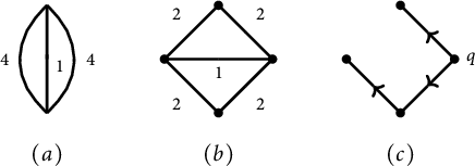
Figure 1: (a) A metric graph $\Gamma $
.(b) A weighted graph model G of
$\Gamma $
.(b) A weighted graph model G of $\Gamma $
.(c) A rooted spanning tree
$\Gamma $
.(c) A rooted spanning tree $(T, q)$
of G and the orientation
$(T, q)$
of G and the orientation ${\mathcal T}_q$
.
${\mathcal T}_q$
.
Given a commutative ring R, it is convenient to define the $1$
-chains with coefficients in R as the free module
$1$
-chains with coefficients in R as the free module
 $$\begin{align*}C_1(G,R) := \frac{\bigoplus_{e \in \mathbb{E}(G)} R e }{ \langle e+\bar{e} \colon e \in {\mathcal O} \rangle}. \end{align*}$$
Note that $\bar {e} = -e$
in
$\bar {e} = -e$
in $C_1(G,R)$
. For each orientation
$C_1(G,R)$
. For each orientation ${\mathcal O}$
on G, we have an isomorphism
${\mathcal O}$
on G, we have an isomorphism $ C_1(G,R) \simeq \bigoplus _{e \in {\mathcal O}} R e$
. For each subset
$ C_1(G,R) \simeq \bigoplus _{e \in {\mathcal O}} R e$
. For each subset ${\mathcal A} \subseteq {\mathbb E}(G)$
, we define its associated
${\mathcal A} \subseteq {\mathbb E}(G)$
, we define its associated $1$
-chain as
$1$
-chain as $\boldsymbol {\gamma }_{\mathcal A} = \sum _{e \in {\mathcal A}} e$
.
$\boldsymbol {\gamma }_{\mathcal A} = \sum _{e \in {\mathcal A}} e$
.
3.2 Metric graphs and models
A metric graph (or metrized graph) is a pair $(\Gamma ,d)$
consisting of a compact connected topological graph
$(\Gamma ,d)$
consisting of a compact connected topological graph $\Gamma $
, together with an inner metric d. Equivalently, if
$\Gamma $
, together with an inner metric d. Equivalently, if $\Gamma $
is not a one-point space, then a metric graph is a compact connected metric space
$\Gamma $
is not a one-point space, then a metric graph is a compact connected metric space $\Gamma $
which has the property that every point has an open neighborhood isometric to a star-shaped set, endowed with the path metric.
$\Gamma $
which has the property that every point has an open neighborhood isometric to a star-shaped set, endowed with the path metric.
The points of $\Gamma $
that have valency different from
$\Gamma $
that have valency different from $2$
are called branch points of
$2$
are called branch points of $\Gamma $
. A vertex set for
$\Gamma $
. A vertex set for $\Gamma $
is a finite set V of points of
$\Gamma $
is a finite set V of points of $\Gamma $
containing all the branch points of
$\Gamma $
containing all the branch points of $\Gamma $
with the property that for each connected component c of
$\Gamma $
with the property that for each connected component c of $\Gamma \setminus V$
, the closure of c in
$\Gamma \setminus V$
, the closure of c in $\Gamma $
is isometric with a closed interval.
$\Gamma $
is isometric with a closed interval.
A vertex set V for $\Gamma $
naturally determines a weighted graph G by setting
$\Gamma $
naturally determines a weighted graph G by setting $V(G)=V$
, and by setting
$V(G)=V$
, and by setting $E(G)$
to be the set of connected components of
$E(G)$
to be the set of connected components of $\Gamma \setminus V$
. We call G a model of
$\Gamma \setminus V$
. We call G a model of $\Gamma $
. An edge segment (based on the choice of a vertex set V) is the closure in
$\Gamma $
. An edge segment (based on the choice of a vertex set V) is the closure in $\Gamma $
of a connected component of
$\Gamma $
of a connected component of $\Gamma \setminus V$
. Note that there is a natural bijective correspondence between
$\Gamma \setminus V$
. Note that there is a natural bijective correspondence between $E(G)$
and the edge segments of
$E(G)$
and the edge segments of $\Gamma $
determined by V. By a small abuse of terminology, we will refer to the elements of
$\Gamma $
determined by V. By a small abuse of terminology, we will refer to the elements of $E(G)$
also as edge segments of
$E(G)$
also as edge segments of $\Gamma $
. Given an edge segment
$\Gamma $
. Given an edge segment $e\subset \Gamma $
(based on the choice of a vertex set V), we denote its boundary
$e\subset \Gamma $
(based on the choice of a vertex set V), we denote its boundary $\partial e \subset V$
by
$\partial e \subset V$
by $\partial e =\{e^-,e^+\}$
. In particular, we will also use the notation
$\partial e =\{e^-,e^+\}$
. In particular, we will also use the notation $\{e^-,e^+\}$
for the boundary set of an edge segment e if there is no (preferred) orientation present. We hope that this does not lead to confusion.
$\{e^-,e^+\}$
for the boundary set of an edge segment e if there is no (preferred) orientation present. We hope that this does not lead to confusion.
Conversely, every weighted graph G naturally determines a metric graph $\Gamma _G$
containing
$\Gamma _G$
containing $V(G)$
by gluing closed intervals
$V(G)$
by gluing closed intervals $[0,\ell (e)]$
for
$[0,\ell (e)]$
for $e \in E(G)$
according to the incidence relations. Note that
$e \in E(G)$
according to the incidence relations. Note that $V(G)$
is naturally a vertex set of
$V(G)$
is naturally a vertex set of $\Gamma _G$
, and the associated model is precisely G. See Figure 1a,b.
$\Gamma _G$
, and the associated model is precisely G. See Figure 1a,b.
3.3 Tropical Jacobians
Let $\Gamma $
be a metric graph. Fix a model G of
$\Gamma $
be a metric graph. Fix a model G of $\Gamma $
. Let
$\Gamma $
. Let ${\mathcal O}=\{e_1,\ldots ,e_m\}$
be a labeling of an orientation
${\mathcal O}=\{e_1,\ldots ,e_m\}$
be a labeling of an orientation ${\mathcal O}$
on G. The real vector space
${\mathcal O}$
on G. The real vector space $ C_1(G,{\mathbb R}) \simeq \bigoplus _{i=1}^m {\mathbb R} e_i$
has a canonical inner product defined by
$ C_1(G,{\mathbb R}) \simeq \bigoplus _{i=1}^m {\mathbb R} e_i$
has a canonical inner product defined by $[ e_i,e_j ]=\delta _i(j)\ell (e_i)$
. Here,
$[ e_i,e_j ]=\delta _i(j)\ell (e_i)$
. Here, $\delta _i$
denotes the delta (Dirac) measure on
$\delta _i$
denotes the delta (Dirac) measure on $\{ 1, 2, \ldots , m\}$
centered at i. The resulting inner product space
$\{ 1, 2, \ldots , m\}$
centered at i. The resulting inner product space $\left ( C_1(G,{\mathbb R}), [\cdot , \cdot ] \right )$
is independent of the choice of
$\left ( C_1(G,{\mathbb R}), [\cdot , \cdot ] \right )$
is independent of the choice of ${\mathcal O}$
and its labeling.
${\mathcal O}$
and its labeling.
The inner product $[ \cdot ,\cdot ]$
restricts to an inner product, also denoted by
$[ \cdot ,\cdot ]$
restricts to an inner product, also denoted by $[ \cdot ,\cdot ]$
, on the homology lattice
$[ \cdot ,\cdot ]$
, on the homology lattice $H =H_1(G,{\mathbb Z}) \subset C_1(G,{\mathbb Z})$
. The pair
$H =H_1(G,{\mathbb Z}) \subset C_1(G,{\mathbb Z})$
. The pair $(H,[ \cdot ,\cdot ])$
is a canonical lattice associated to
$(H,[ \cdot ,\cdot ])$
is a canonical lattice associated to $\Gamma $
(independent of the choice of the model G), and we have a canonical identification
$\Gamma $
(independent of the choice of the model G), and we have a canonical identification $H \simeq H_1(\Gamma ,{\mathbb Z})$
. Note that
$H \simeq H_1(\Gamma ,{\mathbb Z})$
. Note that $H_{{\mathbb R}} \simeq H_1(\Gamma ,{\mathbb R})$
. The associated polarized real torus
$H_{{\mathbb R}} \simeq H_1(\Gamma ,{\mathbb R})$
. The associated polarized real torus $H_1(\Gamma ,{\mathbb R})/H_1(\Gamma ,{\mathbb Z})$
is called the tropical Jacobian of
$H_1(\Gamma ,{\mathbb R})/H_1(\Gamma ,{\mathbb Z})$
is called the tropical Jacobian of $\Gamma $
[Reference Kotani and Sunada23, Reference Mikhalkin and Zharkov25], and denoted by
$\Gamma $
[Reference Kotani and Sunada23, Reference Mikhalkin and Zharkov25], and denoted by $\operatorname {Jac}(\Gamma )$
.
$\operatorname {Jac}(\Gamma )$
.
4 Potential theory on metric graphs
In this section, we closely follow [Reference de Jong and Shokrieh16] and review those results that are needed in this paper.
4.1 Graphs as electrical networks
Let $\Gamma $
be a metric graph, and let G be a model of
$\Gamma $
be a metric graph, and let G be a model of $\Gamma $
. We may think of
$\Gamma $
. We may think of $\Gamma $
(or G) as an electrical network in which each edge
$\Gamma $
(or G) as an electrical network in which each edge $e \in E(G)$
is a resistor having resistance
$e \in E(G)$
is a resistor having resistance $\ell (e)$
. See Figure 2.
$\ell (e)$
. See Figure 2.
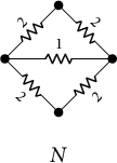
Figure 2: The electrical network N corresponding to the graphs in Figure 1a,b.
When studying the “potential theory” on a metric graph $\Gamma $
, it is convenient to always fix an (arbitrary) model G, and think of it as an electrical network.
$\Gamma $
, it is convenient to always fix an (arbitrary) model G, and think of it as an electrical network.
4.2 Laplacians and j-functions
Let $\Gamma $
be a metric graph, and let G be a model of
$\Gamma $
be a metric graph, and let G be a model of $\Gamma $
. We have the distributional Laplacian operator (see [Reference de Jong and Shokrieh16, Section 3.1])
$\Gamma $
. We have the distributional Laplacian operator (see [Reference de Jong and Shokrieh16, Section 3.1])
 $$\begin{align*}\Delta \colon \operatorname{PL}(\Gamma) \rightarrow \operatorname{DMeas}_{0}(\Gamma),\end{align*}$$
where $\operatorname {PL}(\Gamma )$
is the real vector space consisting of all continuous piecewise affine real valued functions on
$\operatorname {PL}(\Gamma )$
is the real vector space consisting of all continuous piecewise affine real valued functions on $\Gamma $
that can change slope finitely many times on each closed edge segment, and
$\Gamma $
that can change slope finitely many times on each closed edge segment, and $\operatorname {DMeas}_{0}(\Gamma )$
is the real vector space of discrete measures
$\operatorname {DMeas}_{0}(\Gamma )$
is the real vector space of discrete measures $\nu $
on
$\nu $
on $\Gamma $
with
$\Gamma $
with $\nu (\Gamma ) = 0$
. We also have the combinatorial Laplacian operator (see [Reference de Jong and Shokrieh16, Section 3.2])
$\nu (\Gamma ) = 0$
. We also have the combinatorial Laplacian operator (see [Reference de Jong and Shokrieh16, Section 3.2])
 $$\begin{align*}\Delta \colon {\mathcal M}(G) \rightarrow \operatorname{DMeas}_{0}(G),\end{align*}$$
where ${\mathcal M}(G)$
is the real vector space of real-valued functions on
${\mathcal M}(G)$
is the real vector space of real-valued functions on $V(G)$
, and
$V(G)$
, and $\operatorname {DMeas}_{0}(G)$
is the real vector space of discrete measures
$\operatorname {DMeas}_{0}(G)$
is the real vector space of discrete measures $\nu $
on
$\nu $
on $V(G)$
with
$V(G)$
with ${\nu (V(G)) = 0}$
. The distributional Laplacian
${\nu (V(G)) = 0}$
. The distributional Laplacian $\Delta $
and the combinatorial Laplacian
$\Delta $
and the combinatorial Laplacian $\Delta $
are compatible in the sense described in [Reference de Jong and Shokrieh16, Section 3.3]. Moreover, the combinatorial Laplacian on G can be conveniently presented by its Laplacian matrix; let
$\Delta $
are compatible in the sense described in [Reference de Jong and Shokrieh16, Section 3.3]. Moreover, the combinatorial Laplacian on G can be conveniently presented by its Laplacian matrix; let $\{v_1, \ldots , v_n\}$
be a labeling of
$\{v_1, \ldots , v_n\}$
be a labeling of $V(G)$
. The Laplacian matrix
$V(G)$
. The Laplacian matrix ${\mathbf Q}$
associated to G is the
${\mathbf Q}$
associated to G is the $n \times n$
matrix
$n \times n$
matrix ${\mathbf Q} = (q_{ij})$
where, for
${\mathbf Q} = (q_{ij})$
where, for $i \ne j$
, we have
$i \ne j$
, we have $ q_{ij} = - \sum _{e =\{v_i , v_j\} \in E(G)}{{1}/{\ell (e)}} $
. The diagonal entries are determined by forcing the matrix to have zero-sum rows.
$ q_{ij} = - \sum _{e =\{v_i , v_j\} \in E(G)}{{1}/{\ell (e)}} $
. The diagonal entries are determined by forcing the matrix to have zero-sum rows.
The Laplacian matrix of G can also be expressed in terms of the incidence matrix of G. Let $\{v_1, \ldots , v_n\}$
be a labeling of
$\{v_1, \ldots , v_n\}$
be a labeling of $V(G)$
as before. Fix an orientation
$V(G)$
as before. Fix an orientation ${\mathcal O} = \{e_1, \ldots , e_m\}$
on G. The incidence matrix
${\mathcal O} = \{e_1, \ldots , e_m\}$
on G. The incidence matrix ${\mathbf B}$
associated to G is the
${\mathbf B}$
associated to G is the $n \times m$
matrix
$n \times m$
matrix ${\mathbf B}=(b_{ij})$
, where
${\mathbf B}=(b_{ij})$
, where $b_{ij} = +1$
if
$b_{ij} = +1$
if $e_j^{+} = v_i$
and
$e_j^{+} = v_i$
and $b_{ij} = -1$
if
$b_{ij} = -1$
if $e_j^{-} = v_i$
and
$e_j^{-} = v_i$
and $b_{ij} = 0$
otherwise. Let
$b_{ij} = 0$
otherwise. Let ${\mathbf D}$
denote the
${\mathbf D}$
denote the $m \times m$
diagonal matrix with diagonal entries
$m \times m$
diagonal matrix with diagonal entries $\ell (e_i)$
for
$\ell (e_i)$
for $e_i \in {\mathcal O}$
. We have
$e_i \in {\mathcal O}$
. We have ${\mathbf Q} = {\mathbf B} {\mathbf D}^{-1}{\mathbf B}^{\operatorname {T}}$
, where
${\mathbf Q} = {\mathbf B} {\mathbf D}^{-1}{\mathbf B}^{\operatorname {T}}$
, where $(\cdot )^{\operatorname {T}}$
denotes the matrix transpose operation.
$(\cdot )^{\operatorname {T}}$
denotes the matrix transpose operation.
A fundamental solution of the Laplacian is given by j-functions. We follow the notation of [Reference Chinburg and Rumely11]. See [Reference de Jong and Shokrieh16, Section 4] and the references therein for more details. Let $\Gamma $
be a metric graph and fix two points
$\Gamma $
be a metric graph and fix two points $y,z \in \Gamma $
. We denote by
$y,z \in \Gamma $
. We denote by $j_z(\cdot \, , y; \Gamma )$
the unique function in
$j_z(\cdot \, , y; \Gamma )$
the unique function in $\operatorname {PL}(\Gamma )$
satisfying: (i)
$\operatorname {PL}(\Gamma )$
satisfying: (i) $\Delta \left (j_z(\cdot \, , y; \Gamma )\right )= \delta _y - \delta _z$
, and (ii)
$\Delta \left (j_z(\cdot \, , y; \Gamma )\right )= \delta _y - \delta _z$
, and (ii) $j_z(z,y; \Gamma ) = 0$
. If the metric graph
$j_z(z,y; \Gamma ) = 0$
. If the metric graph $\Gamma $
is clear from the context, we write
$\Gamma $
is clear from the context, we write $j_z(x,y)$
instead of
$j_z(x,y)$
instead of $j_z(x,y; \Gamma )$
. The j-function exists and is unique, and satisfies the following basic properties:
$j_z(x,y; \Gamma )$
. The j-function exists and is unique, and satisfies the following basic properties:
-
◇ $j_z(x,y)$
is jointly continuous in all three variables
$x,y,z \in \Gamma $
.
$j_z(x,y)$
is jointly continuous in all three variables
$x,y,z \in \Gamma $
. -
◇
$j_z(x,y) = j_z(y,x)$
. -
◇
$0 \leq j_z(x,y) \leq j_z(x,x)$
. -
◇
$j_z(x,x) = j_x(z,z)$
.


The effective resistance between two points $x, y \in \Gamma $
is
$x, y \in \Gamma $
is $r(x,y) := j_y(x,x)$
. If we want to clarify the underlying metric graph
$r(x,y) := j_y(x,x)$
. If we want to clarify the underlying metric graph $\Gamma $
, we use the notation
$\Gamma $
, we use the notation $r(x,y; \Gamma )$
.
$r(x,y; \Gamma )$
.
Let G be an arbitrary model of $\Gamma $
. One can explicitly compute the quantities
$\Gamma $
. One can explicitly compute the quantities $j_q(p,v) \in {\mathbb R}$
for
$j_q(p,v) \in {\mathbb R}$
for $q,p,v \in V(G)$
using linear algebra (see [Reference Baker and Shokrieh8, Section 3]) as follows. Fix a labeling of
$q,p,v \in V(G)$
using linear algebra (see [Reference Baker and Shokrieh8, Section 3]) as follows. Fix a labeling of $V(G)$
as before, and let
$V(G)$
as before, and let ${\mathbf Q}$
be the corresponding Laplacian matrix. Let
${\mathbf Q}$
be the corresponding Laplacian matrix. Let ${\mathbf Q}_q$
be the
${\mathbf Q}_q$
be the $(n-1)\times (n-1)$
matrix obtained from
$(n-1)\times (n-1)$
matrix obtained from ${\mathbf Q}$
by deleting the row and column corresponding to
${\mathbf Q}$
by deleting the row and column corresponding to $q \in V(G)$
from
$q \in V(G)$
from ${\mathbf Q}$
. It is well known that
${\mathbf Q}$
. It is well known that ${\mathbf Q}_q$
is invertible. Let
${\mathbf Q}_q$
is invertible. Let ${\mathbf L}_q$
be the
${\mathbf L}_q$
be the $n \times n$
matrix obtained from
$n \times n$
matrix obtained from ${\mathbf Q}_q^{-1}$
by inserting zeros in the row and column corresponding to q. One can easily check that
${\mathbf Q}_q^{-1}$
by inserting zeros in the row and column corresponding to q. One can easily check that $ {\mathbf Q}{\mathbf L}_q = {\mathbf I} + {\mathbf R}_q$
, where
$ {\mathbf Q}{\mathbf L}_q = {\mathbf I} + {\mathbf R}_q$
, where ${\mathbf I}$
is the
${\mathbf I}$
is the $n \times n$
identity matrix and
$n \times n$
identity matrix and ${\mathbf R}_q$
has all
${\mathbf R}_q$
has all $-1$
entries in the row corresponding to q and has zeros elsewhere. It follows from the compatibility of the two Laplacians that
$-1$
entries in the row corresponding to q and has zeros elsewhere. It follows from the compatibility of the two Laplacians that ${\mathbf L}_q = (j_q(p,v))_{p,v \in V(G)}$
. The matrix
${\mathbf L}_q = (j_q(p,v))_{p,v \in V(G)}$
. The matrix ${\mathbf L}_q$
is a generalized inverse of
${\mathbf L}_q$
is a generalized inverse of ${\mathbf Q}$
, in the sense that
${\mathbf Q}$
, in the sense that ${\mathbf Q}{\mathbf L}_q{\mathbf Q} = {\mathbf Q}$
.
${\mathbf Q}{\mathbf L}_q{\mathbf Q} = {\mathbf Q}$
.
Remark 4.1 Computing ${\mathbf L}_q$
takes time at most
${\mathbf L}_q$
takes time at most $O(n^\omega )$
, where
$O(n^\omega )$
, where $\omega $
is the exponent for matrix multiplication (currently
$\omega $
is the exponent for matrix multiplication (currently $\omega < 2.38$
).
$\omega < 2.38$
).
4.3 Cross ratios
Let $\Gamma $
be a metric graph and fix
$\Gamma $
be a metric graph and fix $q \in \Gamma $
. As in [Reference de Jong and Shokrieh16], we define the cross ratio function (with respect to the base point q)
$q \in \Gamma $
. As in [Reference de Jong and Shokrieh16], we define the cross ratio function (with respect to the base point q) $\xi _q \colon \Gamma ^4 \rightarrow {\mathbb R}$
by
$\xi _q \colon \Gamma ^4 \rightarrow {\mathbb R}$
by
 $$\begin{align*}\xi_q(x,y , z,w) := j_q(x,z) +j_q(y,w) - j_q(x,w) - j_q(y,z). \end{align*}$$
If we want to clarify the graph $\Gamma $
, we use the notation
$\Gamma $
, we use the notation $\xi _q(x,y , z,w; \Gamma )$
instead. As is observed in [Reference de Jong and Shokrieh16, Remark 6.1(i)], we have the identity
$\xi _q(x,y , z,w; \Gamma )$
instead. As is observed in [Reference de Jong and Shokrieh16, Remark 6.1(i)], we have the identity
 $$\begin{align*}-2\xi_q(x,y , z,w) = r(x, z) + r(y, w) - r(x, w) - r(y, z). \end{align*}$$
Remark 4.2 We borrowed the cross ratio terminology in [Reference de Jong and Shokrieh16] from the book of Baker and Rumely [Reference Baker and Rumely7, Appendix B]. These cross ratios on the Berkovich hyperbolic space and on its natural extension to the Berkovich projective line also play an important role in the work of Favre and Rivera-Letelier [Reference Favre and Rivera-Letelier18, Section 6.3]. The terminology is also justified in the context of Gromov hyperbolic spaces, where this is sometimes called “cross difference” (see, for example, [Reference Väisälä27, Section 4.5]).
Cross ratios satisfy the following basic properties:
-
◇
$\xi (x,y , z,w) := \xi _q(x,y , z,w)$
is independent of the choice of q. -
◇
$\xi (x,y , z,w) = \xi ( z,w,x,y)$
. -
◇
$\xi (y,x , z,w) = - \xi ( x, y, z,w)$
. -
◇
$\xi (x,y , z,w) = \langle \delta _x-\delta _y, \delta _z-\delta _w \rangle _{\operatorname {en}}$
, where
$\langle \cdot , \cdot \rangle _{\operatorname {en}}$
denotes the energy pairing on
$\operatorname {DMeas}_{0}(\Gamma )$
defined by (4.1)
$$ \begin{align} \langle \nu_1 , \nu_2 \rangle_{\operatorname{en}} := \int_{\Gamma \times \Gamma} j_q (x,y) \mathrm{d} \nu_1(x) \mathrm{d} \nu_2(y). \end{align} $$


Example 4.3 The following identities will be useful for our computations.
It follows from $\xi _x(q,x,q,y) = \xi _y(q,x,q,y)$
that
$\xi _x(q,x,q,y) = \xi _y(q,x,q,y)$
that
 $$ \begin{align} r(x, q) - r(y, q) = j_{x}(y , q) - j_{y}(x , q). \end{align} $$
It follows from $\xi _x(x,y,x,q) = \xi _q(x,y,x,q)$
that
$\xi _x(x,y,x,q) = \xi _q(x,y,x,q)$
that
 $$ \begin{align} j_x(y,q) = j_q(x,x) - j_q(x,y). \end{align} $$
It follows from $\xi _x(x,y,x,q) = \xi _y(x,y,x,q)$
that
$\xi _x(x,y,x,q) = \xi _y(x,y,x,q)$
that
 $$ \begin{align} r(x,y) = j_{x}(y , q)+ j_y(x,q). \end{align} $$
It follows from $\xi _x(x,y,x,y) = \xi _q(x,y,x,y)$
that
$\xi _x(x,y,x,y) = \xi _q(x,y,x,y)$
that
 $$ \begin{align} r(x,y) = j_{q}(x , x)+ j_q(y,y) - 2j_q(x,y). \end{align} $$
4.4 Projections
Let G be a weighted graph. Fix an orientation ${\mathcal O}$
. Let T be a spanning tree of G. The weight of T is the product
${\mathcal O}$
. Let T be a spanning tree of G. The weight of T is the product $ w(T) := \prod _{e \not \in T}{\ell (e)}$
. The coweight of T is the product
$ w(T) := \prod _{e \not \in T}{\ell (e)}$
. The coweight of T is the product $ w'(T) := \prod _{e \in T}{\ell ^{-1}(e)}$
. The weight and coweight of G are
$ w'(T) := \prod _{e \in T}{\ell ^{-1}(e)}$
. The weight and coweight of G are $w(G) := \sum _{T}{w(T)}$
and
$w(G) := \sum _{T}{w(T)}$
and $w'(G) := \sum _{T}{w'(T)}$
, where the sums are over all spanning trees of G. The quantity
$w'(G) := \sum _{T}{w'(T)}$
, where the sums are over all spanning trees of G. The quantity $w(G)$
depends only on the underlying metric graph
$w(G)$
depends only on the underlying metric graph $\Gamma $
.
$\Gamma $
.
Let ${\mathbf M}_T$
be the
${\mathbf M}_T$
be the $m \times m$
matrix whose columns are obtained from
$m \times m$
matrix whose columns are obtained from $1$
-chains
$1$
-chains $\operatorname {circ}(T,e)$
associated to fundamental circuits of T, and let
$\operatorname {circ}(T,e)$
associated to fundamental circuits of T, and let ${\mathbf N}_T$
be the
${\mathbf N}_T$
be the $m \times m$
matrix whose columns are obtained from
$m \times m$
matrix whose columns are obtained from $1$
-chains
$1$
-chains $\operatorname {cocirc}(T,e)$
associated to fundamental cocircuits of T (see [Reference de Jong and Shokrieh16, Section 7.2]). Consider the following matrix averages:
$\operatorname {cocirc}(T,e)$
associated to fundamental cocircuits of T (see [Reference de Jong and Shokrieh16, Section 7.2]). Consider the following matrix averages:
 $$\begin{align*}{\mathbf P} = \sum_{T}{\frac{w(T)}{w(G)} {\mathbf M}_T}, \quad {\mathbf P}' = \sum_{T}{\frac{w'(T)}{w'(G)} {\mathbf N}_T}, \end{align*}$$
the sums being over all spanning trees T of G. It is a classical theorem of Kirchhoff [Reference Kirchhoff22] that the matrix of $\pi \colon C_1(G,{\mathbb R}) \twoheadrightarrow H_1(G, {\mathbb R})$
, with respect to
$\pi \colon C_1(G,{\mathbb R}) \twoheadrightarrow H_1(G, {\mathbb R})$
, with respect to ${\mathcal O}$
, is
${\mathcal O}$
, is ${\mathbf P}$
. Similarly, the matrix of
${\mathbf P}$
. Similarly, the matrix of $\pi ' \colon C_1(G,{\mathbb R}) \twoheadrightarrow H_1(G, {\mathbb R})^{\perp }$
, with respect to
$\pi ' \colon C_1(G,{\mathbb R}) \twoheadrightarrow H_1(G, {\mathbb R})^{\perp }$
, with respect to ${\mathcal O}$
, is
${\mathcal O}$
, is $({\mathbf P}')^{\operatorname {T}}$
.
$({\mathbf P}')^{\operatorname {T}}$
.
Let ${\mathbf \Xi }$
be the
${\mathbf \Xi }$
be the $m \times m$
matrix of cross ratios:
$m \times m$
matrix of cross ratios:
 $$\begin{align*}{\mathbf \Xi} := \left(\xi(e^-, e^+ , f^- , f^+) \right)_{e,f \in {\mathcal O}}. \end{align*}$$
Let ${\mathbf L}$
be any generalized inverse of
${\mathbf L}$
be any generalized inverse of ${\mathbf Q}$
(i.e.,
${\mathbf Q}$
(i.e., ${\mathbf Q}{\mathbf L}{\mathbf Q} = {\mathbf Q}$
). Then we have
${\mathbf Q}{\mathbf L}{\mathbf Q} = {\mathbf Q}$
). Then we have ${\mathbf \Xi } = {\mathbf B}^{\operatorname {T}} {\mathbf L} {\mathbf B}$
. It is shown in [Reference de Jong and Shokrieh16, Theorem 7.5] that the matrix of
${\mathbf \Xi } = {\mathbf B}^{\operatorname {T}} {\mathbf L} {\mathbf B}$
. It is shown in [Reference de Jong and Shokrieh16, Theorem 7.5] that the matrix of $\pi \colon C_1(G,{\mathbb R}) \twoheadrightarrow H_1(G, {\mathbb R})$
, with respect to
$\pi \colon C_1(G,{\mathbb R}) \twoheadrightarrow H_1(G, {\mathbb R})$
, with respect to ${\mathcal O}$
, is
${\mathcal O}$
, is ${\mathbf I}- {\mathbf D}^{-1} {\mathbf \Xi }$
, and the matrix of
${\mathbf I}- {\mathbf D}^{-1} {\mathbf \Xi }$
, and the matrix of $\pi ' \colon C_1(G,{\mathbb R}) \twoheadrightarrow H_1(G, {\mathbb R})^{\perp }$
, with respect to
$\pi ' \colon C_1(G,{\mathbb R}) \twoheadrightarrow H_1(G, {\mathbb R})^{\perp }$
, with respect to ${\mathcal O}$
, is
${\mathcal O}$
, is ${\mathbf D}^{-1} {\mathbf \Xi }$
. In particular, for each
${\mathbf D}^{-1} {\mathbf \Xi }$
. In particular, for each $f \in {\mathcal O}$
, we have
$f \in {\mathcal O}$
, we have
-
◇
$\pi (f) = \sum _{e \in {\mathcal O}} {\mathsf F(e,f) e}$
, where (4.6)
$$ \begin{align} \mathsf F(e,f) := \begin{cases} 1-{r(e^-, e^+)}/{\ell(e)}, &\text{ if } e=f,\\ -{\xi(e^-, e^+ ,f^-, f^+)}/{\ell(e)}, &\text{ if } e \ne f. \end{cases} \end{align} $$
-
◇
$\pi '(f) = \sum _{e \in {\mathcal O}} {\mathsf F'(e,f) e}$
, where
$$\begin{align*}\mathsf F'(e,f) = {\xi(e^-, e^+ ,f^-, f^+)}/{\ell(e)}. \end{align*}$$


Moreover, we have equalities:
 $$ \begin{align} {\mathbf P}= {\mathbf I}- {\mathbf D}^{-1} {\mathbf \Xi}, \quad {\mathbf P}' = {\mathbf \Xi} {\mathbf D}^{-1}. \end{align} $$
Definition 4.4 The Foster coefficient of $e \in \mathbb {E}(G)$
is, by definition,
$e \in \mathbb {E}(G)$
is, by definition,
 $$\begin{align*}\mathsf F(e) := \mathsf F(e,e) = 1-\frac{r(e^-, e^+)}{\ell(e)}. \end{align*}$$
Clearly, $\mathsf F(e) = \mathsf F(\bar {e})$
, so
$\mathsf F(e) = \mathsf F(\bar {e})$
, so $\mathsf F(e)$
is also well defined for
$\mathsf F(e)$
is also well defined for $e \in E(G)$
.
$e \in E(G)$
.
Remark 4.5
-
(i) It follows from (4.7) that
the sum being over all spanning trees T of G not containing e.
$$\begin{align*}\mathsf F(e) = \sum_{T \not \ni e} \frac{w(T)}{w(G)}, \end{align*}$$
-
(ii) It is a consequence of “Rayleigh’s monotonicity law” that
$0 \leq \mathsf F(e) < 1$
, and the equality
$\mathsf F(e)=0$
holds if and only if e is a bridge. (See [Reference de Jong and Shokrieh16] and the references therein for more details.)


Fix an arbitrary path $\gamma $
from y to x. Let
$\gamma $
from y to x. Let $\boldsymbol {\gamma }_{yx}$
denote the associated
$\boldsymbol {\gamma }_{yx}$
denote the associated $1$
-chain. Then, by [Reference de Jong and Shokrieh16, Corollary 7.10], we have
$1$
-chain. Then, by [Reference de Jong and Shokrieh16, Corollary 7.10], we have
 $$ \begin{align} r(x,y) = [\boldsymbol{\gamma}_{yx}, \pi'(\boldsymbol{\gamma}_{yx})]. \end{align} $$
Example 4.6 The following observation will be useful for computations. Let $e = \{u,v\}$
denote an edge segment in a metric graph
$e = \{u,v\}$
denote an edge segment in a metric graph $\Gamma $
, and let
$\Gamma $
, and let $p \in e$
be a point with distance x from u and distance
$p \in e$
be a point with distance x from u and distance $\ell (e) - x$
from v. Then, for each point
$\ell (e) - x$
from v. Then, for each point $q \in \Gamma $
, we have
$q \in \Gamma $
, we have
 $$\begin{align*}r(p,q) = \frac{\ell(e)-x}{\ell(e)} r(u,q) + \frac{x}{\ell(e)}r(v,q) + \mathsf F(e) \frac{\left(\ell(e)-x\right)x}{\ell(e)}. \end{align*}$$
This follows, for example, by a direct computation using (4.8). We leave the details to the interested reader.
4.5 Generalized Rayleigh’s laws
We will need the following two corollaries of [Reference de Jong and Shokrieh16, Theorem B]. Let $\Gamma $
be a metric graph. Let e be an edge segment of
$\Gamma $
be a metric graph. Let e be an edge segment of $\Gamma $
with boundary points
$\Gamma $
with boundary points $\partial e = \{e^-, e^+\}$
. Let
$\partial e = \{e^-, e^+\}$
. Let $\Gamma /e$
denote the metric graph obtained by contracting e (equivalently, by setting
$\Gamma /e$
denote the metric graph obtained by contracting e (equivalently, by setting $\ell (e) = 0$
). Then
$\ell (e) = 0$
). Then
 $$ \begin{align} j_z(x,y; \Gamma/e) = j_z(x,y; \Gamma) - \frac{\xi(x,z , e^-, e^+; \Gamma) \, \xi(y,z , e^-, e^+; \Gamma)}{r(e^-, e^+; \Gamma)}, \end{align} $$
and
 $$ \begin{align} r(x,y; \Gamma/e) =r(x,y; \Gamma) - \frac{\xi(x,y , e^-, e^+; \Gamma) ^2}{r(e^-, e^+; \Gamma)}. \end{align} $$
4.6 Contractions and models
Let G be a weighted graph, and let $e \in E(G)$
be an edge of G. We denote by
$e \in E(G)$
be an edge of G. We denote by $G/e$
the weighted graph obtained from G by contracting the edge e and removing all loops that might be created in the process. Assume that G is a model of the metric graph
$G/e$
the weighted graph obtained from G by contracting the edge e and removing all loops that might be created in the process. Assume that G is a model of the metric graph $\Gamma $
. In particular, we may view e as an edge segment of
$\Gamma $
. In particular, we may view e as an edge segment of $\Gamma $
. We then observe that, for
$\Gamma $
. We then observe that, for $x, y, z, w \in V(G)$
, the cross ratio
$x, y, z, w \in V(G)$
, the cross ratio $\xi (x,y,z,w;\Gamma /e)$
measured on
$\xi (x,y,z,w;\Gamma /e)$
measured on $\Gamma /e$
is equal to the cross ratio
$\Gamma /e$
is equal to the cross ratio $\xi (x,y,z,w;G/e)$
measured on (the metric graph canonically associated to)
$\xi (x,y,z,w;G/e)$
measured on (the metric graph canonically associated to) $G/e$
. A similar remark pertains to the j-function
$G/e$
. A similar remark pertains to the j-function $j_z(x,y;\Gamma /e)$
and the effective resistance function
$j_z(x,y;\Gamma /e)$
and the effective resistance function $r(x,y;\Gamma /e)$
. We leave the details to the reader.
$r(x,y;\Gamma /e)$
. We leave the details to the reader.
5 Calculus of random spanning trees
In this section, we study two functions arising from random spanning trees.
Definition 5.1 Let G be a model of a metric graph $\Gamma $
. For edges
$\Gamma $
. For edges $e = \{e^-, e^+\}$
and
$e = \{e^-, e^+\}$
and $f = \{f^-, f^+\}$
of G, we define
$f = \{f^-, f^+\}$
of G, we define
 $$\begin{align*}\mathrm P (e,f) := \begin{cases} {r(e^-, e^+; G)}/{\ell(e)}, &\text{ if}\ e=f,\\ {r(e^-, e^+; G)}/{\ell(e)} \times {r(f^-, f^+; G/e)}/{\ell(f)}, &\text{ if}\ e\ne f. \end{cases} \end{align*}$$
We use the notation $\mathrm P(e):= \mathrm P (e,e)$
. If we want to clarify the underlying model G, we use the notations
$\mathrm P(e):= \mathrm P (e,e)$
. If we want to clarify the underlying model G, we use the notations $\mathrm P(e,f; G)$
and
$\mathrm P(e,f; G)$
and $\mathrm P(e; G)$
.
$\mathrm P(e; G)$
.
By Definition 4.4 and Remark 4.5(i), we know
 $$ \begin{align} \mathrm P(e) = 1-\mathsf F(e) = \sum_{T \ni e} \frac{w(T)}{w(G)}, \end{align} $$
the sum being over all spanning trees T of G containing e. So $\mathrm P(e)$
is the probability of e being present in a random spanning tree, where a spanning tree T is chosen with probability
$\mathrm P(e)$
is the probability of e being present in a random spanning tree, where a spanning tree T is chosen with probability ${w(T)}/{w(G)}$
.
${w(T)}/{w(G)}$
.
A similar probabilistic interpretation holds for $\mathrm P (e,f)$
when
$\mathrm P (e,f)$
when $e\ne f$
. Namely, since
$e\ne f$
. Namely, since $\mathrm P (e,f) = \mathrm P(e; G) \mathrm P(f; G/e)$
, it represents the probability of both e and f being present in a random spanning tree. In other words,
$\mathrm P (e,f) = \mathrm P(e; G) \mathrm P(f; G/e)$
, it represents the probability of both e and f being present in a random spanning tree. In other words,
 $$ \begin{align} \mathrm P(e,f) = \sum_{T \ni e,f} \frac{w(T)}{w(G)}. \end{align} $$
It follows that $\mathrm P(e,f) = \mathrm P(f,e)$
. One can use (4.10) (alternatively, the “transfer–current theorem”—see [Reference Lyons and Peres24, Section 4.2]) to compute
$\mathrm P(e,f) = \mathrm P(f,e)$
. One can use (4.10) (alternatively, the “transfer–current theorem”—see [Reference Lyons and Peres24, Section 4.2]) to compute $\mathrm P(e,f)$
directly in terms of invariants of G.
$\mathrm P(e,f)$
directly in terms of invariants of G.
Definition 5.2
-
(i) Let
${\mathfrak s} \colon V(G) \rightarrow {\mathbb R}$
be the function defined by sending
$p \in V(G)$
to the sum being over all edges e incident to p in G (i.e., the star of p).
$$\begin{align*}{\mathfrak s}(p) := \sum_{e=\{p , x\}} \mathrm P(e), \end{align*}$$
-
(ii) Let
${\mathfrak t} \colon V(G) \times E(G) \rightarrow {\mathbb R}$
be the function defined by sending
$(p , e)$
to the sum being over all edges f incident to p in G.
$$\begin{align*}{\mathfrak t}(p, e) := \sum_{f=\{p , x\}} \mathrm P(e, f), \end{align*}$$


Proposition 5.3 Fix a vertex $q \in V(G)$
. We have
$q \in V(G)$
. We have
 $$\begin{align*}{\mathfrak s}(p) = \sum_{e=\{p , x\}} \frac{r(x,q) - r(p,q)}{\ell(e)} + 2 - 2\, \delta_q(p), \end{align*}$$
the sum being over all edges $e \in E(G)$
incident to p.
$e \in E(G)$
incident to p.
Proof By (4.5), we may write $r(p,x) = j_q(x,x) - j_q(p,p) + 2 (j_q(p,p) - j_q(x,p))$
. Therefore,
$r(p,x) = j_q(x,x) - j_q(p,p) + 2 (j_q(p,p) - j_q(x,p))$
. Therefore,
 $$\begin{align*}\begin{aligned} {\mathfrak s}(p) &= \sum_{e=\{p , x\}} \frac{r(p,x)}{\ell(e)} \\[4pt] &= \sum_{e=\{p , x\}} \frac{ j_q(x,x) - j_q(p,p)}{\ell(e)} + 2 \sum_{e=\{p , x\}}\frac{j_q(p,p) - j_q(x,p)}{\ell(e)} \\[4pt] &= \sum_{e=\{p , x\}} \frac{ j_q(x,x) - j_q(p,p)}{\ell(e)} + 2 \Delta \left( j_q(\cdot,p)\right) (p)\\[4pt] &= \sum_{e=\{p , x\}} \frac{ j_q(x,x) - j_q(p,p)}{\ell(e)} + 2 (\delta_p(p) - \delta_q(p)). \end{aligned}\\[-46pt] \end{align*}$$
▪
Recall from Section 4.6 the weighted graph $G/e$
obtained by contracting the edge
$G/e$
obtained by contracting the edge $e=\{u,v\} \in E(G)$
and removing all loops that might be created in the process. Let
$e=\{u,v\} \in E(G)$
and removing all loops that might be created in the process. Let $\mathrm {Par}(e) \subseteq E(G)$
denote the set of all edges parallel to e (i.e., connecting u and v). We make the identification
$\mathrm {Par}(e) \subseteq E(G)$
denote the set of all edges parallel to e (i.e., connecting u and v). We make the identification $E(G/e) = E(G)\backslash \mathrm {Par}(e)$
, and the two vertices
$E(G/e) = E(G)\backslash \mathrm {Par}(e)$
, and the two vertices $u, v \in V(G)$
will be identified with a single vertex
$u, v \in V(G)$
will be identified with a single vertex $v_e \in V(G/e)$
(see Figure 3), and
$v_e \in V(G/e)$
(see Figure 3), and $V(G) \backslash \{u,v\} = V(G/e) \backslash \{v_e\}$
.
$V(G) \backslash \{u,v\} = V(G/e) \backslash \{v_e\}$
.
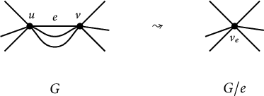
Figure 3: Contracting the edge $e = \{u,v\}$
.
$e = \{u,v\}$
.
Theorem 5.4 Fix a vertex $q \in V(G)$
. Let
$q \in V(G)$
. Let $p \in V(G)$
and
$p \in V(G)$
and $e= \{u,v\} \in E(G)$
. Then
$e= \{u,v\} \in E(G)$
. Then
 $$\begin{align*}\begin{aligned} {\mathfrak t}(p,e) &= \frac{r(u,v; G)}{\ell(e)} \sum_{\substack{f=\{p , x\} \\ f \in E(G)\backslash \mathrm{Par}(e)}} \frac{r(x,q; G/e) - r(p,q; G/e)}{\ell(f)} \\[4pt] &\quad +2 \frac{r(u,v; G)}{\ell(e)} \left(1- \delta_q(p) - \frac{\xi(u,v,u,q; G)}{r(u,v; G)} \delta_u(p)- \frac{\xi(v,u,v,q; G)}{r(u,v; G)}\delta_v(p) \right). \end{aligned} \end{align*}$$
The sum is over all edges $f \in E(G) \backslash \mathrm {Par}(e)$
incident to p in G.
$f \in E(G) \backslash \mathrm {Par}(e)$
incident to p in G.
Proof By definition,
 $$\begin{align*}\mathrm P (e,f) = \frac{r(u,v; G)}{\ell(e)} \mathrm P(f; G/e).\end{align*}$$
If $p \not \in \{u,v\}$
, the result follows immediately from Proposition 5.3:
$p \not \in \{u,v\}$
, the result follows immediately from Proposition 5.3:
 $$\begin{align*}{\mathfrak t}(p,e) = \frac{r(u,v; G)}{\ell(e)} \left(\sum_{\substack{f=\{p , x\} \\ f \in E(G)}} \frac{r(x,q; G/e) - r(p,q; G/e)}{\ell(e)} + 2 - 2\, \delta_q(p)\right), \end{align*}$$
the sum being over all edges $f \in E(G)$
incident to p in G (equivalently, all edges
$f \in E(G)$
incident to p in G (equivalently, all edges $f \in E(G/e)$
incident to p in
$f \in E(G/e)$
incident to p in $G/e$
).
$G/e$
).
So, by symmetry, it remains to show the equality for $p= u$
. Recall that we denote the vertex obtained by identifying u and v in
$p= u$
. Recall that we denote the vertex obtained by identifying u and v in $G/e$
by
$G/e$
by $v_e$
(Figure 3). As in the proof of Proposition 5.3, we first compute
$v_e$
(Figure 3). As in the proof of Proposition 5.3, we first compute
 $$ \begin{align} \begin{aligned} {\mathfrak t}(u,e) &= \frac{r(u,v; G)}{\ell(e)} \left(\sum_{\substack{f=\{u , x\} \\ f \in E(G)\backslash \mathrm{Par}(e)}} \frac{ j_q(x,x;G/e) - j_q(v_e,v_e;G/e)}{\ell(f)} \right) \\[4pt] &\quad + 2 \frac{r(u,v; G)}{\ell(e)}\left(\sum_{\substack{f=\{u , x\} \\ f \in E(G)\backslash \mathrm{Par}(e)}}\frac{j_q(v_e,v_e;G/e) - j_q(x,v_e;G/e)}{\ell(f)} \right), \end{aligned} \end{align} $$
where the sums are over all edges $f \in E(G) \backslash \mathrm {Par}(e)$
incident to u in G. Unlike in the proof of Proposition 5.3, we cannot interpret the second sum as the Laplacian of the j-function on
$f \in E(G) \backslash \mathrm {Par}(e)$
incident to u in G. Unlike in the proof of Proposition 5.3, we cannot interpret the second sum as the Laplacian of the j-function on $G/e$
because the summation is not over all edges incident to
$G/e$
because the summation is not over all edges incident to $v_e$
in
$v_e$
in $G/e$
(e.g., in Figure 3, only edges on the left of
$G/e$
(e.g., in Figure 3, only edges on the left of $v_e$
appear in the summation). We proceed by “lifting” the problem to G using generalized Rayleigh’s laws (4.9) and (4.10). We find
$v_e$
appear in the summation). We proceed by “lifting” the problem to G using generalized Rayleigh’s laws (4.9) and (4.10). We find
 $$\begin{align*}\begin{aligned} &\frac{j_q(v_e,v_e;G/e) - j_q(x,v_e;G/e)}{\ell(f)} = \frac{j_q(u,u;G) - j_q(x,u;G)}{\ell(f)}\\[4pt] &\quad + \frac{\xi(u,v,u,q;G)}{r(u,v;G)}\left( \frac{\xi(u,v,x,q;G) - \xi(u,v,u,q;G)}{\ell(f)}\right). \end{aligned} \end{align*}$$
It is easily checked that the right-hand side is zero for $x=v$
. Moreover, by the definition of cross ratios, we compute
$x=v$
. Moreover, by the definition of cross ratios, we compute
 $$\begin{align*}\xi(u,v,x,q;G) - \xi(u,v,u,q;G) = \xi(u,v,x,u;G).\end{align*}$$
So we have
 $$ \begin{align} \begin{aligned} &\sum_{\substack{f=\{u , x\} \\ f \in E(G)\backslash \mathrm{Par}(e)}}\frac{j_q(v_e,v_e;G/e) - j_q(x,v_e;G/e)}{\ell(f)} = \sum_{\substack{f=\{u , x\} \\ f \in E(G)}} \frac{j_q(u,u;G) - j_q(x,u;G)}{\ell(f)}\\[4pt] &\quad + \frac{\xi(u,v,u,q;G)}{r(u,v;G)} \sum_{\substack{f=\{u , x\} \\ f \in E(G)}} \frac{\xi(u,v,x,u;G)}{\ell(f)}. \end{aligned} \end{align} $$
As in the proof of Proposition 5.3, we have
 $$ \begin{align} \begin{aligned} \sum_{\substack{f=\{u , x\} \\ f \in E(G)}} \frac{j_q(u,u;G) - j_q(x,u;G)}{\ell(f)} &= \Delta\left(j_q (\cdot , u)\right)(u)\\ &= \delta_u(u)-\delta_q(u) = 1- \delta_q(u). \end{aligned} \end{align} $$
By expanding with respect to the base point q, we also compute
 $$ \begin{align} \begin{aligned} \sum_{\substack{f=\{u , x\} \\ f \in E(G)}} \frac{\xi(u,v,x,u;G)}{\ell(f)} &= \sum_{\substack{f=\{u , x\} \\ f \in E(G)}} \frac{j_q(v,u;G) - j_q(v,x;G)}{\ell(f)} \\[4pt] &\quad - \sum_{\substack{f=\{u , x\} \\ f \in E(G)}} \frac{j_q(u,u;G) - j_q(u,x;G)}{\ell(f)} \\[4pt] &= \Delta\left(j_q (v , \cdot)\right)(u) - \Delta\left(j_q (u , \cdot)\right)(u) \\[4pt] &= \left(\delta_v(u) - \delta_q(u) \right) - \left(\delta_u(u) - \delta_q(u) \right) \\[4pt] &= -1. \end{aligned} \end{align} $$
The result for $p=u$
follows by putting together (5.3)–(5.6).▪
$p=u$
follows by putting together (5.3)–(5.6).▪
6 Energy levels of rooted spanning trees
In this section, we prove a very subtle identity for cross ratios (Theorem 6.3).
6.1 Energy levels
Recall that a rooted spanning tree $(T, q)$
of G comes with a preferred orientation
$(T, q)$
of G comes with a preferred orientation ${\mathcal T}_q \subseteq \mathbb {E}(G)$
, where all edges are oriented away from q on the spanning tree T (see Section 3.1).
${\mathcal T}_q \subseteq \mathbb {E}(G)$
, where all edges are oriented away from q on the spanning tree T (see Section 3.1).
Definition 6.1 We define the energy level of a rooted spanning tree $(T, q)$
to be
$(T, q)$
to be
 $$\begin{align*}\boldsymbol{\varrho}(T, q) := \sum_{e,f \in {\mathcal T}_q} \xi(e^-, e^+, f^-, f^+). \end{align*}$$
The following result is a justification for our terminology, and is useful in our later computation. Let $\deg _T(v)$
denote the number of edges incident with
$\deg _T(v)$
denote the number of edges incident with $v \in V(G)$
in the spanning tree T. Consider the canonical element
$v \in V(G)$
in the spanning tree T. Consider the canonical element $ \nu _{(T,q)} \in \operatorname {DMeas}_{0}(G)$
associated to the rooted spanning tree
$ \nu _{(T,q)} \in \operatorname {DMeas}_{0}(G)$
associated to the rooted spanning tree $(T, q)$
of G defined by
$(T, q)$
of G defined by
 $$\begin{align*}\nu_{(T,q)} = \sum_{v\in V(G)} \left(\deg_T(v) - 2\right) \delta_v + 2 \delta_q. \end{align*}$$
Lemma 6.2 We have
 $$ \begin{align}\qquad \boldsymbol{\varrho}(T, q ) = \langle \nu_{(T,q)}, \nu_{(T,q)} \rangle_{\operatorname{en}} = \sum_{v,w \in V(G)} \left(\deg_T(v) - 2\right)\left(\deg_T(w) - 2\right) j_q(v,w). \end{align} $$
Proof By the definition of the preferred orientation ${\mathcal T}_q \subseteq \mathbb {E}(G)$
, we have
${\mathcal T}_q \subseteq \mathbb {E}(G)$
, we have
 $$\begin{align*}\sum_{e \in {\mathcal T}_q} \left(\delta_{e^-} - \delta_{e^+}\right) = \nu_{(T,q)}. \end{align*}$$
This is because every vertex $v \ne q$
has exactly one incoming edge and
$v \ne q$
has exactly one incoming edge and $\deg _T(v) - 1$
outgoing edges in
$\deg _T(v) - 1$
outgoing edges in ${\mathcal T}_q$
. At q, however, there is no incoming edge in
${\mathcal T}_q$
. At q, however, there is no incoming edge in ${\mathcal T}_q$
.
${\mathcal T}_q$
.
The result now follows directly from bilinearity of the energy pairing:
 $$\begin{align*}\begin{aligned} \boldsymbol{\varrho}(T, q) &= \sum_{e,f \in {\mathcal T}_q} \xi(e^-, e^+, f^-, f^+) =\sum_{e,f \in {\mathcal T}_q} \langle \delta_{e^-} - \delta_{e^+}, \delta_{f^-} - \delta_{f^+}\rangle_{\operatorname{en}} \\[4pt] &=\ \langle \, \sum_{e \in {\mathcal T}_q} \left(\delta_{e^-} - \delta_{e^+}\right),\sum_{f \in {\mathcal T}_q}\left( \delta_{f^-} - \delta_{f^+}\right) \, \rangle_{\operatorname{en}} = \langle \nu_{(T,q)}, \nu_{(T,q)} \rangle_{\operatorname{en}}. \end{aligned} \end{align*}$$
The second equality in (6.1) follows from (4.1), because $j_q(\cdot , q) = j_q (q, \cdot ) = 0$
.▪
$j_q(\cdot , q) = j_q (q, \cdot ) = 0$
.▪
6.2 The average of energy levels
We can now state the most technical ingredient in computing tropical moments of tropical Jacobians.
Theorem 6.3 Fix a vertex $q \in V(G)$
. We have the equality
$q \in V(G)$
. We have the equality
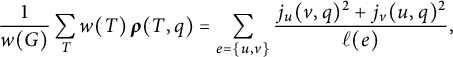 $$\begin{align*}\frac{1}{w(G)}\sum_T {w(T) \, {\boldsymbol{\varrho}}(T, q)} = \sum_{e = \{u,v\}}\frac{j_{u}(v, q)^2 + j_{v}(u, q)^2}{\ell(e)}, \end{align*}$$
where the sum on the left is over all spanning trees T of G, and the sum on the right is over all edges $e \in E(G)$
.
$e \in E(G)$
.
Lemma 6.4 Let $(T,q)$
be a rooted spanning tree of G. We have the equality
$(T,q)$
be a rooted spanning tree of G. We have the equality
 $$\begin{align*}\begin{aligned} \boldsymbol{\varrho}(T, q) &= 4 \sum_{x,y \in V(G)} j_q(x,y) - 4 \sum_{e \in T} \sum_{x \in V(G)} \left(j_q(e^-, x)+j_q(e^+, x)\right) \\[4pt] &\quad + \sum_{e,f \in T}\left(j_q(e^-, f^-)+j_q(e^+, f^+)+j_q(e^-, f^+)+j_q(e^+, f^-) \right). \end{aligned} \end{align*}$$
Proof The result follows from Lemma 6.2, and an application of a (generalized) handshaking lemma: for each $\psi \in {\mathcal M}(G)$
, we have
$\psi \in {\mathcal M}(G)$
, we have
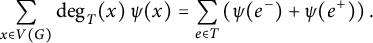 $$\begin{align*}\sum_{x \in V(G)} \deg_T(x) \,\psi (x) = \sum_{e \in T} \left(\psi(e^-)+\psi(e^+)\right).\\[-48pt] \end{align*}$$
▪
Lemma 6.5 Fix a vertex $q \in V(G)$
. We have the equality
$q \in V(G)$
. We have the equality
 $$\begin{align*}\begin{aligned} & \frac{1}{w(G)}\sum_T {w(T) \, {\boldsymbol{\varrho}}(T, q)} = 4\!\! \!\!\!\! \!\sum_{x,y \in V(G)}\!\!\!\!\!\! j_q(x,y) -4\!\!\!\!\!\sum_{e \in E(G)} \sum_{x \in V(G)} \!\!\!\left(j_q(e^-, x)+j_q(e^+, x)\right) \mathrm P(e) \\[4pt] &\quad +\sum_{e,f \in E(G)}\left(j_q(e^-, f^-)+j_q(e^+, f^+)+j_q(e^-, f^+)+j_q(e^+, f^-)\right) \mathrm P(e,f). \end{aligned} \end{align*}$$
Proof This follows from Lemma 6.4: one only needs to change the order of summations and use (5.1) and (5.2).▪
To prove the next two results, it is convenient to work with matrices. We fix labelings $V(G) = \{v_1, \ldots , v_n\}$
and
$V(G) = \{v_1, \ldots , v_n\}$
and $E(G) = \{e_1, \ldots , e_m\}$
, and we introduce the following matrices:
$E(G) = \{e_1, \ldots , e_m\}$
, and we introduce the following matrices:
-
◇
${\mathbf 1}_n \in {\mathbb R}^n$
and
${\mathbf 1}_m \in {\mathbb R}^m$
denote the all-ones vectors. -
◇
$\boldsymbol {\delta }_v \in {\mathbb R}^n$
(resp.
$\boldsymbol {\delta }_e \in {\mathbb R}^m$
) denotes the characteristic vector of
$v \in V(G)$
(resp.
$e \in E(G)$
). -
◇
${\mathbf A} = (h_{ij})$
denotes the
$n \times m$
unsigned incidence matrix of G, where
$h_{ij} = 1$
if
$e_j^+ = v_i$
or
$e_j^- = v_i$
, and
$h_{ij} = 0$
otherwise. -
◇
${\mathbf X}$
is the
$n \times n$
diagonal matrix with diagonal
$(i,i)$
-entries
$j_q(v_i, v_i) = r(v_i, q)$
. -
◇
${\mathbf Y}$
is the
$m \times m$
diagonal matrix with diagonal
$(i,i)$
-entries
$\mathrm P(e_i)$
. -
◇
${\mathbf Z}$
is the
$m \times m$
matrix whose diagonal entries are zero, and the
$(i,j)$
-entries (
$i\ne j$
) are
$\mathrm P(e_i, e_j)$
.


We will also use the matrices ${\mathbf Q}$
,
${\mathbf Q}$
, ${\mathbf L}_q$
,
${\mathbf L}_q$
, ${\mathbf R}_q$
, and
${\mathbf R}_q$
, and ${\mathbf I}$
introduced in Section 4.2.
${\mathbf I}$
introduced in Section 4.2.
Lemma 6.6 We have the equality
 $$ \begin{align} \sum_{e \in E(G)} \sum_{x \in V(G)} \left(j_q(e^-, x)+j_q(e^+, x)\right)\mathrm P(e) = 2 \sum_{x,y \in V(G)} j_q(x,y) - \sum_{x \in V(G)} j_q(x,x). \end{align} $$
Proof We start by writing the left-hand side of (6.2) in terms of our matrices:
 $$\begin{align*}\sum_{e \in E(G)} \sum_{x \in V(G)} \left(j_q(e^-, x)+j_q(e^+, x)\right)\mathrm P(e) = {\mathbf 1}_n^{\operatorname{T}}{\mathbf L}_q {\mathbf A} {\mathbf Y} {\mathbf 1}_m. \end{align*}$$
By definitions, we observe ${\mathbf A} {\mathbf Y} {\mathbf 1}_m = \left ({\mathfrak s}(v_1), \ldots , {\mathfrak s}(v_n)\right )^{\operatorname {T}}$
. So, by Proposition 5.3, we have
${\mathbf A} {\mathbf Y} {\mathbf 1}_m = \left ({\mathfrak s}(v_1), \ldots , {\mathfrak s}(v_n)\right )^{\operatorname {T}}$
. So, by Proposition 5.3, we have
 $$\begin{align*}{\mathbf A} {\mathbf Y} {\mathbf 1}_m = -{\mathbf Q} {\mathbf X} {\mathbf 1}_n + 2\left({\mathbf 1}_n - \boldsymbol{\delta}_q\right). \end{align*}$$
Therefore,
 $$\begin{align*}{\mathbf 1}_n^{\operatorname{T}}{\mathbf L}_q {\mathbf A} {\mathbf Y} {\mathbf 1}_m = - {\mathbf 1}_n^{\operatorname{T}}{\mathbf L}_q{\mathbf Q} {\mathbf X} {\mathbf 1}_n + 2 {\mathbf 1}_n^{\operatorname{T}}{\mathbf L}_q {\mathbf 1}_n -2{\mathbf 1}_n^{\operatorname{T}}{\mathbf L}_q \boldsymbol{\delta}_q. \end{align*}$$
Note that ${\mathbf L}_q \boldsymbol {\delta }_q = \mathbf {0}$
and
${\mathbf L}_q \boldsymbol {\delta }_q = \mathbf {0}$
and ${\mathbf L}_q{\mathbf Q} = {\mathbf I}+{\mathbf R}_q^{\operatorname {T}}$
(see Section 4.2). We also have
${\mathbf L}_q{\mathbf Q} = {\mathbf I}+{\mathbf R}_q^{\operatorname {T}}$
(see Section 4.2). We also have ${\mathbf R}_q^{\operatorname {T}} {\mathbf X} = \mathbf {0}$
. Therefore,
${\mathbf R}_q^{\operatorname {T}} {\mathbf X} = \mathbf {0}$
. Therefore,
 $$\begin{align*}{\mathbf 1}_n^{\operatorname{T}}{\mathbf L}_q {\mathbf A} {\mathbf Y} {\mathbf 1}_m = 2 {\mathbf 1}_n^{\operatorname{T}}{\mathbf L}_q {\mathbf 1}_n - {\mathbf 1}_n^{\operatorname{T}} {\mathbf X} {\mathbf 1}_n, \end{align*}$$
which is the right-hand side of (6.2).▪
For our next computation, it is convenient to use the notion of Hadamard–Schur products of matrices: for two $k \times m$
matrices
$k \times m$
matrices $A , B$
, the Hadamard–Schur product, denoted by
$A , B$
, the Hadamard–Schur product, denoted by $A \circ B$
, is a matrix of the same dimension as A and B with entries given by
$A \circ B$
, is a matrix of the same dimension as A and B with entries given by $\left (A \circ B\right )_{ij} = (A)_{ij}(B)_{ij}$
.
$\left (A \circ B\right )_{ij} = (A)_{ij}(B)_{ij}$
.
One useful (and easy to prove) fact about Hadamard–Schur products is the following:
 $$ \begin{align} {\mathbf 1}_k^{\operatorname{T}} \left( A \circ B\right) {\mathbf 1}_m= \operatorname{Trace} \left({A^{\operatorname{T}}B}\right).\end{align} $$
Lemma 6.7 We have the equality
 $$\begin{align*}\begin{aligned} &\sum_{e,f \in E(G)}\left(j_q(e^-, f^-)+j_q(e^+, f^+)+j_q(e^-, f^+)+j_q(e^+, f^-)\right) \mathrm P(e,f) \\[4pt] &\quad =\sum_{e = \{u,v\}}\frac{j_{u}(v, q)^2 + j_{v}(u, q)^2}{\ell(e)} +4 \sum_{x,y \in V(G)} j_q(x,y) -4 \sum_{x \in V(G)} j_q(x,x). \end{aligned} \end{align*}$$
Proof We first write
 $$ \begin{align} \begin{aligned} &\qquad\sum_{e,f \in E(G)} \left(j_q(e^-, f^-)+j_q(e^+, f^+)+j_q(e^-, f^+)+j_q(e^+, f^-)\right) \mathrm P(e,f)\\[4pt] &\qquad\quad = \sum_{e\in E(G)} \left(j_q(e^-, e^-)+j_q(e^+, e^+)+2j_q(e^-, e^+)\right) \mathrm P(e)\\[4pt] &\qquad\qquad + \sum_{\substack{e,f \in E(G)\\ e \ne f}} \left(j_q(e^-, f^-)+j_q(e^+, f^+)+j_q(e^-, f^+)+j_q(e^+, f^-)\right) \mathrm P(e,f). \end{aligned} \end{align} $$
We write the second sum in (6.4) in terms of our matrices:
 $$ \begin{align} \begin{aligned} & \sum_{\substack{e,f \in E(G)\\ e \ne f}} \left(j_q(e^-, f^-)+j_q(e^+, f^+)+j_q(e^-, f^+)+j_q(e^+, f^-)\right) \mathrm P(e,f) \\[4pt] &\quad = {\mathbf 1}_m^{\operatorname{T}}\left( \left({\mathbf A}^{\operatorname{T}} {\mathbf L}_q {\mathbf A} \right) \circ {\mathbf Z}\right) {\mathbf 1}_m. \end{aligned} \end{align} $$
By (6.3), we know
 $$\begin{align*}{\mathbf 1}_m^{\operatorname{T}}\left( \left({\mathbf A}^{\operatorname{T}} {\mathbf L}_q {\mathbf A} \right) \circ {\mathbf Z}\right) {\mathbf 1}_m = \operatorname{Trace} \left( {\mathbf A}^{\operatorname{T}} {\mathbf L}_q {\mathbf A} {\mathbf Z} \right) = \sum_{e\in E(G)} \boldsymbol{\delta}_e^{\operatorname{T}} \left({\mathbf A}^{\operatorname{T}} {\mathbf L}_q {\mathbf A} {\mathbf Z} \right) \boldsymbol{\delta}_e. \end{align*}$$
By definitions, one observes ${\mathbf A} {\mathbf Z} \boldsymbol {\delta }_e = \left ({\mathfrak t}(v_1, e), \ldots , {\mathfrak t}(v_n, e)\right )^{\operatorname {T}}$
. Let
${\mathbf A} {\mathbf Z} \boldsymbol {\delta }_e = \left ({\mathfrak t}(v_1, e), \ldots , {\mathfrak t}(v_n, e)\right )^{\operatorname {T}}$
. Let
 $$\begin{align*}e=\{u,v\} \ \ , \ \ \beta_u = \frac{\xi(u,v,u,q)}{r(u,v)} \ \ , \ \ \beta_v = \frac{\xi(v,u,v,q)}{r(u,v)} \ \ , \ \ \mathrm P(e) = \frac{r(u,v)}{\ell(e)}. \end{align*}$$
Theorem 5.4 states
 $$\begin{align*}{\mathbf A} {\mathbf Z} \boldsymbol{\delta}_e = \mathrm P(e) \left(-{\mathbf Q} \widetilde{{\mathbf X}} {\mathbf 1}_n +2\left({\mathbf 1}_n - \boldsymbol{\delta}_q - \beta_u \boldsymbol{\delta}_u - \beta_v \boldsymbol{\delta}_v\right) \right). \end{align*}$$
Here, $\widetilde {{\mathbf X}}$
is the
$\widetilde {{\mathbf X}}$
is the $n \times n$
diagonal matrix with diagonal
$n \times n$
diagonal matrix with diagonal $(i,i)$
-entries
$(i,i)$
-entries $j_q(v_i, v_i; G/e)$
for
$j_q(v_i, v_i; G/e)$
for $v_i \not \in \{u,v\}$
. The diagonal entries corresponding to both u and v are
$v_i \not \in \{u,v\}$
. The diagonal entries corresponding to both u and v are $j_q(v_e, v_e; G/e)$
. Thus, we find
$j_q(v_e, v_e; G/e)$
. Thus, we find
 $$\begin{align*}\boldsymbol{\delta}_e^{\operatorname{T}} \left({\mathbf A}^{\operatorname{T}} {\mathbf L}_q {\mathbf A} {\mathbf Z} \right) \boldsymbol{\delta}_e = \mathrm P(e) \left(\boldsymbol{\delta}_u+\boldsymbol{\delta}_v\right)^{\operatorname{T}} {\mathbf L}_q \left(-{\mathbf Q} \widetilde{{\mathbf X}} {\mathbf 1}_n +2\left({\mathbf 1}_n - \boldsymbol{\delta}_q - \beta_u \boldsymbol{\delta}_u - \beta_v \boldsymbol{\delta}_v\right) \right). \end{align*}$$
Note that ${\mathbf L}_q \boldsymbol {\delta }_q = \mathbf {0}$
,
${\mathbf L}_q \boldsymbol {\delta }_q = \mathbf {0}$
, ${\mathbf L}_q{\mathbf Q} = {\mathbf I}+{\mathbf R}_q^{\operatorname {T}}$
, and
${\mathbf L}_q{\mathbf Q} = {\mathbf I}+{\mathbf R}_q^{\operatorname {T}}$
, and ${\mathbf R}_q^{\operatorname {T}} \widetilde {{\mathbf X}} = \mathbf {0}$
. We obtain
${\mathbf R}_q^{\operatorname {T}} \widetilde {{\mathbf X}} = \mathbf {0}$
. We obtain
 $$ \begin{align} \begin{aligned} &\boldsymbol{\delta}_e^{\operatorname{T}} \left({\mathbf A}^{\operatorname{T}} {\mathbf L}_q {\mathbf A} {\mathbf Z} \right) \boldsymbol{\delta}_e =\mathrm P(e) \left(\boldsymbol{\delta}_u+\boldsymbol{\delta}_v\right)^{\operatorname{T}} \left(-\widetilde{{\mathbf X}} {\mathbf 1}_n + 2 {\mathbf L}_q \left({\mathbf 1}_n - \beta_u \boldsymbol{\delta}_u -\beta_v \boldsymbol{\delta}_v\right) \right) \\[4pt] &= -\mathrm P(e) \left(j_q(v_e,v_e; G/e)+j_q(v_e,v_e; G/e)\right) +2 \mathrm P(e) \! \! \sum_{x \in V(G)}\left(j_q(u,x) + j_q(v, x)\right)\\[4pt] &\ \ \ -2 \left(\frac{\xi(u,v,u,q)}{\ell(e)}\left(j_q(u,u) + j_q(v, u)\right) +\frac{\xi(v,u,v,q)}{\ell(e)} \left(j_q(u,v) + j_q(v, v)\right)\right). \end{aligned} \end{align} $$
We now use our generalized Rayleigh’s law (4.10) twice and write everything in terms of invariants of G:
 $$ \begin{align} \begin{aligned} j_q(v_e,v_e; G/e) &= j_q(u,u) - \frac{\xi(u,q,u,v)^2}{r(u,v)} = j_q(u,u) - \frac{j_u(v,q)^2}{r(u,v)},\\ j_q(v_e,v_e; G/e) &= j_q(v,v) - \frac{\xi(v,q,u,v)^2}{r(u,v)} = j_q(v,v) - \frac{j_v(u,q)^2}{r(u,v)}. \end{aligned} \end{align} $$
We also use the definition of cross ratios to compute
 $$ \begin{align} \xi(u,v,u,q) = j_q(u,u)- j_q(u,v) \ , \ \xi(v,u,v,q) = j_q(v,v)- j_q(u,v). \end{align} $$
Putting together (6.4)–(6.8), with a simple computation, we obtain
 $$ \begin{align} \begin{aligned} &\qquad\sum_{e,f \in E(G)} \left(j_q(e^-, f^-)+j_q(e^+, f^+)+j_q(e^-, f^+)+j_q(e^+, f^-)\right) \mathrm P(e,f) \\[4pt] &\quad\qquad = \sum_{e = \{u,v\}}\frac{j_{u}(v, q)^2 + j_{v}(u, q)^2}{\ell(e)} + 2 \sum_{e = \{u,v\}} \sum_{x \in V(G)} \mathrm P(e)\left( j_q(u,x)+j_q(v,x)\right) \\[4pt] &\quad\qquad\quad + 2 \sum_{e =\{u,v\}} \mathrm P(e) j_q(u,v) -2 \sum_{e = \{u,v\}} \frac{j_q(u,u)^2 +j_q(v,v)^2 -2j_q(u,v)^2}{\ell(e)}. \end{aligned} \end{align} $$
By Lemma 6.6, the second term in (6.9) is simplified as
 $$ \begin{align} \sum_{e = \{u,v\}} \sum_{x \in V(G)} \mathrm P(e)\left( j_q(u,x)+j_q(v,x)\right) = 2\sum_{x,y \in V(G)} j_q(x,y) - \sum_{x \in V(G)} j_q(x,x). \end{align} $$
The third and fourth terms in (6.9) are simplified as follows:
 $$ \begin{align} \\ & \sum_{e =\{u,v\}} \mathrm P(e) j_q(u,v) - \sum_{e = \{u,v\}} \frac{j_q(u,u)^2 +j_q(v,v)^2 -2j_q(u,v)^2}{\ell(e)} \nonumber \\[4pt] &= \!\! \sum_{e =\{u,v\}} \! \left(\frac{j_q(u,u)\!+\!j_q(v,v)\!-\!2j_q(u,v)}{\ell(e)}j_q(u,v) -\frac{j_q(u,u)^2 \!+\!j_q(v,v)^2 \!-\!2j_q(u,v)^2}{\ell(e)} \right) \nonumber \\&= - \sum_{e =\{u,v\}}\left( j_q(u,u) \frac{j_q(u,u)- j_q(u,v)}{\ell(e)} + j_q(v,v) \frac{j_q(v,v)- j_q(u,v)}{\ell(e)}\right) \nonumber \\[4pt] &= -\sum_{x \in V(G)} j_q(x,x) \sum_{f = \{x, y\}} \frac{j_q(x,x) -j_q(x,y)}{\ell(f)} = -\sum_{x \in V(G)} j_q(x,x) \Delta(j_q(x, \cdot))(x) \nonumber \\[4pt] &= -\sum_{x \in V(G)} j_q(x,x) \left(\delta_x(x) - \delta_q(x) \right) = -\sum_{x \in V(G)} j_q(x,x). \nonumber \end{align} $$
For the first equality, we used (4.5). The third equality is by a (generalized) handshaking lemma. The result now follows by putting together (6.9)–(6.11).▪
6.3 Average of energy levels, a variation
For our main application, we will need the following slight variation of Theorem 6.3. Let $\pi \colon C_1(G, {\mathbb R}) \twoheadrightarrow H_1(G, {\mathbb R})$
denote the orthogonal projection (as defined in Section 4.4).
$\pi \colon C_1(G, {\mathbb R}) \twoheadrightarrow H_1(G, {\mathbb R})$
denote the orthogonal projection (as defined in Section 4.4).
Definition 6.8 We define the center of a rooted spanning tree $(T, q)$
to be
$(T, q)$
to be
 $$\begin{align*}\sigma_T := \frac{1}{2}\sum_{e \in {\mathcal T}_q} {\pi(e)}. \end{align*}$$
Theorem 6.9 We have the equality
 $$\begin{align*}\frac{1}{w(G)}\sum_T w(T)[\sigma_T, \sigma_T] = \frac{1}{4}\sum_{e = \{u,v\}} \left(r(u,v) - \frac{j_{u}( v, q)^2 + j_{v}( u, q)^2}{\ell(e)}\right), \end{align*}$$
where the sum on the left is over all spanning trees T of G, and the sum on the right is over all edges $e \in E(G)$
.
$e \in E(G)$
.
Proof Using (4.6) and Definition 6.1, we compute
 $$ \begin{align} \\ &[\sigma_T, \sigma_T] = \frac{1}{4} [\sum_{e \in {\mathcal T}_q} {\pi(e)}, \sum_{e \in {\mathcal T}_q} {\pi(e)}]= \frac{1}{4} \left( \sum_{e \in {\mathcal T}_q} [\pi(e), \pi(e)] + \sum_{\substack{e,f \in {\mathcal T}_q\\ e \ne f}} [\pi(e), \pi(f)]\right) \nonumber \\[4pt] &=\frac{1}{4} \left( \! \sum_{e \in T} \mathsf F(e) \ell(e) + \!\!\! \sum_{\substack{e,f \in {\mathcal T}_q\\ e \ne f}} \mathsf F(e,f) \ell(e) \! \right) \! \! =\frac{1}{4} \left(\! \sum_{e \in T} \mathsf F(e) \ell(e) - \!\!\! \sum_{\substack{e,f \in {\mathcal T}_q\\ e \ne f}} \xi(e^-, e^+, f^-, f^+) \right) \nonumber \\[4pt] &=\frac{1}{4} \left( \sum_{e \in T} \mathsf F(e) \ell(e) +\sum_{e \in {\mathcal T}_q} r(e^-, e^+) - \!\!\!\sum_{\substack{e,f \in {\mathcal T}_q}} \xi(e^-, e^+, f^-, f^+) \right) \nonumber \\[4pt] &=\frac{1}{4} \sum_{\substack{e \in T\\ e=\{u,v\}}} \left(\mathsf F(e) \ell(e) +r(u, v)\right) - \frac{1}{4} {\boldsymbol{\varrho}}(T, q). \nonumber \end{align} $$
By Definition 4.4 and (5.1) and by changing the order of summations, we compute
 $$ \begin{align} \begin{aligned} & \sum_T \frac{w(T)}{w(G)} \sum_{\substack{e \in T\\ e=\{u,v\}}} \left(\mathsf F(e) \ell(e) +r(u, v)\right) = \sum_{e=\{u,v\}} \left(\mathsf F(e) \ell(e) +r(u, v)\right) \sum_{T \ni e} \frac{w(T)}{w(G)}\\[4pt] &\quad = \sum_{e=\{u,v\}} \left(\mathsf F(e) \ell(e) +r(u, v)\right) \mathrm P(e)=\sum_{e=\{u,v\}} r(u,v). \end{aligned} \end{align} $$
The result now follows from (6.12), (6.13), and Theorem 6.3.▪
7 Combinatorics of Voronoi polytopes
Throughout this section, we fix a metric graph $\Gamma $
and a model G. We are interested in the combinatorics of the lattice
$\Gamma $
and a model G. We are interested in the combinatorics of the lattice $\left (H_1(G, {\mathbb Z}), [\cdot , \cdot ]\right )$
. More specifically, we study the combinatorics of the Voronoi polytopes
$\left (H_1(G, {\mathbb Z}), [\cdot , \cdot ]\right )$
. More specifically, we study the combinatorics of the Voronoi polytopes $\operatorname {Vor}(\lambda )$
(as defined in Section 2.2) for the lattice
$\operatorname {Vor}(\lambda )$
(as defined in Section 2.2) for the lattice $\left (H_1(G, {\mathbb Z}), [\cdot , \cdot ]\right )$
. Since
$\left (H_1(G, {\mathbb Z}), [\cdot , \cdot ]\right )$
. Since $\operatorname {Vor} ( \lambda ) = \operatorname {Vor}(0)+ \lambda $
for all
$\operatorname {Vor} ( \lambda ) = \operatorname {Vor}(0)+ \lambda $
for all $\lambda \in H_1(G, {\mathbb Z})$
, it suffices to understand the Voronoi polytope
$\lambda \in H_1(G, {\mathbb Z})$
, it suffices to understand the Voronoi polytope $\operatorname {Vor}(0)$
around the origin.
$\operatorname {Vor}(0)$
around the origin.
Let $\operatorname {Vol}\left (\cdot \right )$
denote the volume measure induced by the bilinear form
$\operatorname {Vol}\left (\cdot \right )$
denote the volume measure induced by the bilinear form $[ \cdot , \cdot ]$
on
$[ \cdot , \cdot ]$
on $H_1(G, {\mathbb R})$
. Let
$H_1(G, {\mathbb R})$
. Let $w(G)$
be the weight of G (as in Section 4.4). Put
$w(G)$
be the weight of G (as in Section 4.4). Put $g=\dim _{\mathbb R} H_1(G,{\mathbb R})$
.
$g=\dim _{\mathbb R} H_1(G,{\mathbb R})$
.
Lemma 7.1 $\operatorname {Vol}\left (\operatorname {Vor}(0)\right ) = \sqrt {w(G) }$
.
$\operatorname {Vol}\left (\operatorname {Vor}(0)\right ) = \sqrt {w(G) }$
.
Proof The Voronoi polytopes $\{\operatorname {Vor}(0)+ \lambda \colon \lambda \in H_1(G, {\mathbb Z})\}$
induce a periodic polytopal decomposition of
$\{\operatorname {Vor}(0)+ \lambda \colon \lambda \in H_1(G, {\mathbb Z})\}$
induce a periodic polytopal decomposition of $H_1(G, {\mathbb R})$
. Therefore,
$H_1(G, {\mathbb R})$
. Therefore, $\operatorname {Vor}(0)$
, up to some identifications on its boundary, gives a fundamental domain for the translation action of
$\operatorname {Vor}(0)$
, up to some identifications on its boundary, gives a fundamental domain for the translation action of $H_1(G, {\mathbb Z})$
on
$H_1(G, {\mathbb Z})$
on $H_1(G, {\mathbb R})$
. Therefore,
$H_1(G, {\mathbb R})$
. Therefore, $\operatorname {Vol}\left (\operatorname {Vor}(0)\right ) = \sqrt {\det ({\mathbf G})}$
where
$\operatorname {Vol}\left (\operatorname {Vor}(0)\right ) = \sqrt {\det ({\mathbf G})}$
where ${\mathbf G}$
is any Gram matrix for the lattice
${\mathbf G}$
is any Gram matrix for the lattice $\left (H_1(G, {\mathbb Z}), [\cdot , \cdot ]\right )$
.
$\left (H_1(G, {\mathbb Z}), [\cdot , \cdot ]\right )$
.
Fix an orientation ${\mathcal O}$
on G, and fix a spanning tree T of G. It is well known that
${\mathcal O}$
on G, and fix a spanning tree T of G. It is well known that $\{\operatorname {circ}(T,e) \colon e \in {\mathcal O} \backslash T\}$
is a basis for
$\{\operatorname {circ}(T,e) \colon e \in {\mathcal O} \backslash T\}$
is a basis for $H_1(G, {\mathbb R})$
. Let
$H_1(G, {\mathbb R})$
. Let ${\mathbf C}_T$
denote the totally unimodular
${\mathbf C}_T$
denote the totally unimodular $g \times m$
matrix whose rows correspond to these basis elements. Then a Gram matrix for the lattice
$g \times m$
matrix whose rows correspond to these basis elements. Then a Gram matrix for the lattice $\left (H_1(G, {\mathbb Z}), [\cdot , \cdot ]\right )$
is
$\left (H_1(G, {\mathbb Z}), [\cdot , \cdot ]\right )$
is ${\mathbf G}_T = {\mathbf C}_T {\mathbf D} {\mathbf C}_T^{\operatorname {T}}$
. The result now follows from a standard application of the Cauchy–Binet formula for determinants.▪
${\mathbf G}_T = {\mathbf C}_T {\mathbf D} {\mathbf C}_T^{\operatorname {T}}$
. The result now follows from a standard application of the Cauchy–Binet formula for determinants.▪
Remark 7.2 A geometric proof of Lemma 7.1 can be found in [Reference An, Baker, Kuperberg and Shokrieh2, Section 5].
Let $\pi \colon C_1(G, {\mathbb R}) \twoheadrightarrow H_1(G, {\mathbb R})$
denote the orthogonal projection (as defined in Section 4.4). Each finite collection of
$\pi \colon C_1(G, {\mathbb R}) \twoheadrightarrow H_1(G, {\mathbb R})$
denote the orthogonal projection (as defined in Section 4.4). Each finite collection of $1$
-chains
$1$
-chains $V = \{{\mathbf v}_1 , \ldots , {\mathbf v}_k\} \subset C_1(G,{\mathbb R})$
generates a zonotope
$V = \{{\mathbf v}_1 , \ldots , {\mathbf v}_k\} \subset C_1(G,{\mathbb R})$
generates a zonotope ${\mathcal Z}(V)$
defined as
${\mathcal Z}(V)$
defined as
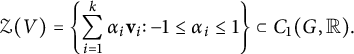 $$\begin{align*}{\mathcal Z}(V) = \left\{ \sum_{i=1}^k \alpha_i {\mathbf v}_i \colon -1 \leq \alpha_i \leq 1 \right\} \subset C_1(G,{\mathbb R}). \end{align*}$$
Proposition 7.3 Fix an orientation ${\mathcal O}$
on G. Then
${\mathcal O}$
on G. Then
 $$\begin{align*}\operatorname{Vor}(0) = \frac{1}{2} \, {\mathcal Z} \left(\{ \pi(e) \colon e \in {\mathcal O}\}\right). \end{align*}$$
Proof This is well known. To the best of our knowledge, this was first proved in [Reference Oda and Seshadri26, Proposition 5.2]. See also [Reference Dutour Sikirić, Schürmann and Vallentin17, Theorem 2] for a different proof.▪
Fix an orientation ${\mathcal O}$
on G. Let T be a spanning tree of G. We define
${\mathcal O}$
on G. Let T be a spanning tree of G. We define
 $$\begin{align*}{\mathcal C}_T := \frac{1}{2} {\mathcal Z} \left( \{ \pi(e) \colon e \in {\mathcal O} \backslash T \}\right). \end{align*}$$
Note that ${\mathcal C}_T$
is independent of the choice of
${\mathcal C}_T$
is independent of the choice of ${\mathcal O}$
.
${\mathcal O}$
.
Lemma 7.4
-
(a)
${\mathcal C}_T$
is a g-dimensional parallelotope. Equivalently,
$\{\pi (e) \colon e \in {\mathcal O} \backslash T\}$
is a basis for
$H_1(G, {\mathbb R})$
. -
(b)
$\operatorname {Vol}({\mathcal C}_T) = w(T)/\sqrt {w(G)}$
.


Proof (a) Note that, for $e,e' \in {\mathcal O} \backslash T$
, we have
$e,e' \in {\mathcal O} \backslash T$
, we have $[\pi (e) , \operatorname {circ}(T,e')] = \ell (e) \delta _e(e')$
. It is well known that
$[\pi (e) , \operatorname {circ}(T,e')] = \ell (e) \delta _e(e')$
. It is well known that $\{\operatorname {circ}(T,e) \colon e \in {\mathcal O} \backslash T\}$
is a basis for
$\{\operatorname {circ}(T,e) \colon e \in {\mathcal O} \backslash T\}$
is a basis for $H_1(G, {\mathbb R})$
.
$H_1(G, {\mathbb R})$
.
(b) This is proved in [Reference An, Baker, Kuperberg and Shokrieh2, Proposition 5.4].▪
Now, fix $q \in V(G)$
. Recall (see Section 3.1) that the rooted spanning tree
$q \in V(G)$
. Recall (see Section 3.1) that the rooted spanning tree $(T, q)$
comes with a preferred orientation
$(T, q)$
comes with a preferred orientation ${\mathcal T}_q \subseteq \mathbb {E}(G)$
(where edges are oriented away from q on the spanning tree T). Let
${\mathcal T}_q \subseteq \mathbb {E}(G)$
(where edges are oriented away from q on the spanning tree T). Let $\sigma _T := \frac {1}{2}\sum _{e \in {\mathcal T}_q} {\pi (e)}$
be the center of
$\sigma _T := \frac {1}{2}\sum _{e \in {\mathcal T}_q} {\pi (e)}$
be the center of $(T,q)$
(Definition 6.8). We now state and prove the main result of this section.
$(T,q)$
(Definition 6.8). We now state and prove the main result of this section.
Theorem 7.5 The collection of parallelotopes
 $$\begin{align*}\{\sigma_T + {\mathcal C}_T \colon T \text{ is a spanning tree of } G\}\end{align*}$$
induces a polytopal decomposition of $\operatorname {Vor}(0)$
:
$\operatorname {Vor}(0)$
:
-
(i)
$\operatorname {Vor}(0) = \bigcup _{T} \left (\sigma _T + {\mathcal C}_T \right )$
, the union being over all spanning trees T of G. -
(ii) If
$T \ne T'$
are two spanning trees such that is nonempty, then
$$\begin{align*}{\mathcal F} := \left(\sigma_T + {\mathcal C}_T \right) \cap \left(\sigma_{T'} + {\mathcal C}_{T'} \right)\end{align*}$$
$\mathcal {F} $
is a face of both
$\left (\sigma _T + {\mathcal C}_T \right )$
and
$\left (\sigma _{T'} + {\mathcal C}_{T'} \right )$
.


Proof It follows from Proposition 7.3 that, for all spanning trees T of G, we have
 $$ \begin{align} \sigma_T + {\mathcal C}_T \subseteq \operatorname{Vor}(0). \end{align} $$
Moreover, by Lemmas 7.1 and 7.4(b), we know
 $$ \begin{align} \sum_T{\operatorname{Vol}\left(\sigma_T + {\mathcal C}_T \right)} = \operatorname{Vol}\left(\operatorname{Vor}(0)\right), \end{align} $$
the sum being over all spanning trees T of G.
Next, we describe how these parallelotopes can intersect each other. Let $T \ne T'$
be two spanning trees. We choose an orientation
$T \ne T'$
be two spanning trees. We choose an orientation ${\mathcal O}$
on G that agrees with
${\mathcal O}$
on G that agrees with ${\mathcal T}_q$
for
${\mathcal T}_q$
for $e\in T$
, disagrees with
$e\in T$
, disagrees with ${\mathcal T}^{\prime }_q$
for
${\mathcal T}^{\prime }_q$
for $e \in T' \backslash T$
, and is arbitrary outside
$e \in T' \backslash T$
, and is arbitrary outside $T \cup T'$
. We may partition
$T \cup T'$
. We may partition ${\mathcal O}$
into the following (possibly empty) subsets:
${\mathcal O}$
into the following (possibly empty) subsets:
 $$\begin{align*}\begin{aligned} {\mathcal S}_1 := {\mathcal T}_q \, \backslash \left( {\mathcal T}^{\prime}_q \cup \overline{{\mathcal T}^{\prime}_q}\right), \,\, {\mathcal S}_2 &:= \overline{{\mathcal T}^{\prime}_q} \, \backslash \left( {\mathcal T}_q \cup \overline{{\mathcal T}_q}\right) , \,\, {\mathcal S}_3 := {\mathcal T}_q \, \cap \overline{{\mathcal T}^{\prime}_q} \,\, , \,\, {\mathcal S}_4 := {\mathcal T}_q \, \cap {\mathcal T}^{\prime}_q,\\ {\mathcal S}_5 &:= {\mathcal O} \backslash \left({\mathcal S}_1 \cup {\mathcal S}_2 \cup {\mathcal S}_3 \cup {\mathcal S}_4 \right)\kern-1.5pt. \end{aligned} \end{align*}$$
We can now describe the corresponding parallelotopes as follows:
 $$\begin{align*}\sigma_T + {\mathcal C}_T = \frac{1}{2} \, {\mathcal Z} \left(\{ \pi(e) \colon e \in {\mathcal S}_2 \cup {\mathcal S}_5\}\right) + \frac{1}{2}\sum_{e \in {\mathcal S}_1 \cup {\mathcal S}_3 \cup {\mathcal S}_4} \pi(e), \end{align*}$$
 $$\begin{align*}\sigma_{T'} + {\mathcal C}_{T'} = \frac{1}{2} \, {\mathcal Z} \left(\{ \pi(e) \colon e \in {\mathcal S}_1 \cup {\mathcal S}_5\}\right) - \frac{1}{2}\sum_{e \in {\mathcal S}_2 \cup {\mathcal S}_3} \pi(e) + \frac{1}{2}\sum_{e \in {\mathcal S}_4} \pi(e). \end{align*}$$
Consider the oriented subgraph ${\mathcal D} := {\mathcal S}_1 \cup {\mathcal S}_2 \cup {\mathcal S}_3$
. Note that the oriented subgraph
${\mathcal D} := {\mathcal S}_1 \cup {\mathcal S}_2 \cup {\mathcal S}_3$
. Note that the oriented subgraph ${\mathcal D}$
is obtained from the edge set
${\mathcal D}$
is obtained from the edge set $T\cup T'$
by deleting those edges in
$T\cup T'$
by deleting those edges in $T\cap T'$
that have the same orientation in
$T\cap T'$
that have the same orientation in ${\mathcal T}_q$
and in
${\mathcal T}_q$
and in ${\mathcal T}^{\prime }_q$
, and by orienting the remaining edges according to
${\mathcal T}^{\prime }_q$
, and by orienting the remaining edges according to ${\mathcal O}$
. One can extend
${\mathcal O}$
. One can extend ${\mathcal D}$
to a totally cyclic (also known as strongly connected) subgraph of G, after possibly adding some oriented edges to
${\mathcal D}$
to a totally cyclic (also known as strongly connected) subgraph of G, after possibly adding some oriented edges to ${\mathcal D}$
chosen from the (unoriented) edges of
${\mathcal D}$
chosen from the (unoriented) edges of $\mathcal {S}_4$
. This is because
$\mathcal {S}_4$
. This is because ${\mathcal D}$
, by construction, has no directed cocircuit. This implies that there exists a vector
${\mathcal D}$
, by construction, has no directed cocircuit. This implies that there exists a vector ${\mathbf v} \in H_1(G, {\mathbb R})$
such that
${\mathbf v} \in H_1(G, {\mathbb R})$
such that
 $$\begin{align*}\begin{aligned} [{\mathbf v} , \pi(e)] &> 0, \quad \quad \text{if } e \in {\mathcal S}_1 \cup {\mathcal S}_2 \cup {\mathcal S}_3,\\ [{\mathbf v} , \pi(e)] &= 0, \quad \quad \text{if } e \in {\mathcal S}_5. \end{aligned} \end{align*}$$
To see this, consider the oriented (cographic) hyperplane arrangement with normal vectors $\{\pi (e) \colon e \in {\mathcal O}\}$
in the vector space
$\{\pi (e) \colon e \in {\mathcal O}\}$
in the vector space $H_1(G, {\mathbb R})$
. It is well known (see, e.g., [Reference Greene and Zaslavsky19, Lemma 8.2]) that there is a one-to-one correspondence between cells of this hyperplane arrangement and totally cyclic subgraphs of G (see also [Reference Amini1]). Our desired vector
$H_1(G, {\mathbb R})$
. It is well known (see, e.g., [Reference Greene and Zaslavsky19, Lemma 8.2]) that there is a one-to-one correspondence between cells of this hyperplane arrangement and totally cyclic subgraphs of G (see also [Reference Amini1]). Our desired vector ${\mathbf v}$
is any vector in the cell corresponding to any totally cyclic extension of
${\mathbf v}$
is any vector in the cell corresponding to any totally cyclic extension of ${\mathcal D}$
.
${\mathcal D}$
.
Consider the function ${\mathfrak h} \colon H_1(G, {\mathbb R}) \rightarrow {\mathbb R}$
defined by
${\mathfrak h} \colon H_1(G, {\mathbb R}) \rightarrow {\mathbb R}$
defined by
 $$\begin{align*}{\mathfrak h}(z) = [{\mathbf v} , z + \sum_{e \in {\mathcal S}_2}{\frac{1}{2}\pi(e)} - \sum_{e \in {\mathcal S}_1 \cup {\mathcal S}_4}{\frac{1}{2}\pi(e)}]. \end{align*}$$
Let ${\mathcal F}= \left (\sigma _T + {\mathcal C}_T \right ) \cap \left (\sigma _{T'} + {\mathcal C}_{T'} \right )$
. We compute
${\mathcal F}= \left (\sigma _T + {\mathcal C}_T \right ) \cap \left (\sigma _{T'} + {\mathcal C}_{T'} \right )$
. We compute
 $$\begin{align*}{\mathfrak h}\left( \sigma_T + {\mathcal C}_T \right) = \{ 0 \leq x \leq \sum_{e \in {\mathcal S}_2} [{\mathbf v}, \pi(e) ] \} + \frac{1}{2}\sum_{e \in {\mathcal S}_3} [{\mathbf v}, \pi(e) ] \subseteq {\mathbb R}_{\geq 0}, \end{align*}$$
 $$\begin{align*}{\mathfrak h}\left( \sigma_{T'} + {\mathcal C}_{T'} \right) = \{ - \sum_{e \in {\mathcal S}_1} [{\mathbf v}, \pi(e) ] \leq x \leq 0\} - \frac{1}{2}\sum_{e \in {\mathcal S}_3} [{\mathbf v}, \pi(e) ] \subseteq {\mathbb R}_{\leq 0}. \end{align*}$$
-
• If
${\mathcal S}_3 \ne \emptyset $
, then
${\mathfrak h}\left ( \sigma _T + {\mathcal C}_T \right )\cap {\mathfrak h}\left ( \sigma _{T'} + {\mathcal C}_{T'} \right ) = \emptyset $
and, therefore,
${\mathcal F}= \emptyset $
. -
• If
${\mathcal S}_3 = \emptyset $
, then
${\mathfrak h}\left ( \sigma _T + {\mathcal C}_T \right ) \cap {\mathfrak h}\left ( \sigma _{T'} + {\mathcal C}_{T'} \right ) = \{0\}$
. Consider the hyperplane
$\mathcal {H} = {\mathfrak h}^{-1}(0)$
in
$H_1(G, {\mathbb R})$
. One computes
$$\begin{align*}\begin{aligned} &\mathcal{H} \cap \left(\sigma_T + {\mathcal C}_T \right) = \mathcal{H} \cap \left(\sigma_{T'} + {\mathcal C}_{T'}\right) \\[4pt] &= \frac{1}{2} \, {\mathcal Z} \left(\{ \pi(e) \colon e \in {\mathcal S}_5\}\right) + \frac{1}{2}\sum_{e \in {\mathcal S}_1 \cup {\mathcal S}_4} \pi(e) - \frac{1}{2}\sum_{e \in {\mathcal S}_2} \pi(e)\\[4pt] &= {\mathcal F}. \end{aligned} \end{align*}$$


The result now follows from these intersection patterns, together with (7.1) and (7.2).▪
8 The tropical moment of a tropical Jacobian
In this section, we prove our promised potential theoretic expression for the tropical moment of a tropical Jacobian.
Theorem 8.1 Let $\Gamma $
be a metric graph. Fix a model G of
$\Gamma $
be a metric graph. Fix a model G of $\Gamma $
, and fix a point
$\Gamma $
, and fix a point $q \in V(G)$
. Then
$q \in V(G)$
. Then
 $$\begin{align*}I(\operatorname{Jac}(\Gamma)) = \frac{1}{12}\sum_{e} {\mathsf F(e)^2 \ell(e) + \frac{1}{4}\sum_{e = \{u,v\}} \left(r(u,v) - \frac{j_{u}( v, q)^2 + j_{v}( u, q)^2}{\ell(e)}\right)}, \end{align*}$$
where the sums are over all edges $e \in E(G)$
.
$e \in E(G)$
.
Proof Recall
 $$\begin{align*}I(\operatorname{Jac}(\Gamma)) = \int_{\operatorname{Vor}(0)} [ z,z ] \, \mathrm{d} \mu_L(z), \end{align*}$$
where $\mu _L$
is the Lebesgue measure on
$\mu _L$
is the Lebesgue measure on $H_1(G, {\mathbb R})$
, normalized to have
$H_1(G, {\mathbb R})$
, normalized to have $\mu _L(\operatorname {Vor}(0)) = 1$
. By Theorem 7.5, we obtain
$\mu _L(\operatorname {Vor}(0)) = 1$
. By Theorem 7.5, we obtain
 $$ \begin{align} I(\operatorname{Jac}(\Gamma)) = \sum_T \int_{\sigma_T + {\mathcal C}_T} [ z,z ] \, \mathrm{d} \mu_L(z), \end{align} $$
the sums being over all spanning trees T of G. We also have
 $$ \begin{align} \begin{aligned} \int_{\sigma_T + {\mathcal C}_T} [ z,z ] \, \mathrm{d} \mu_L(z) &= \int_{{\mathcal C}_T} [ y+\sigma_T, y+\sigma_T ] \, \mathrm{d} \mu_L(y)\\[4pt] &= \int_{{\mathcal C}_T} \left( [ y, y]+2[\sigma_T, y]+[\sigma_T, \sigma_T] \right) \, \mathrm{d} \mu_L(y)\\[4pt] &= \int_{{\mathcal C}_T} [ y, y] \, \mathrm{d} \mu_L(y) + \int_{{\mathcal C}_T} [\sigma_T, \sigma_T] \, \mathrm{d} \mu_L(y). \end{aligned} \end{align} $$
The last equality is because ${{\mathcal C}_T}$
is centrally symmetric and
${{\mathcal C}_T}$
is centrally symmetric and $[\sigma _T, y]$
is odd.
$[\sigma _T, y]$
is odd.
By Lemmas 7.1 and 7.4(b), we have
 $$ \begin{align} \int_{{\mathcal C}_T} [\sigma_T, \sigma_T] \, \mathrm{d} \mu_L(y) = \frac{\operatorname{Vol}({\mathcal C}_T)}{\operatorname{Vol}\left(\operatorname{Vor}(0)\right)} [\sigma_T, \sigma_T] = \frac{w(T)}{w(G)}[\sigma_T, \sigma_T]. \end{align} $$
On the other hand,
 $$ \begin{align} \begin{aligned} \int_{{\mathcal C}_T} [ y, y] \, \mathrm{d} \mu_L&(y)= \frac{\operatorname{Vol}({\mathcal C}_T)}{\operatorname{Vol}\left(\operatorname{Vor}(0)\right)} \int_{[-\frac{1}{2}, \frac{1}{2}]^g} [\sum_{e \not\in T} \alpha_e \pi(e) , \sum_{e \not\in T} \alpha_e \pi(e)] \, \mathrm{d} \boldsymbol{\alpha} \\[4pt] &= \frac{w(T)}{w(G)} \int_{[-\frac{1}{2}, \frac{1}{2}]^g} \left( \sum_{\substack{e,f \not\in T\\ e \ne f}} \alpha_e \alpha_{f} [\pi(e), \pi(f)] + \sum_{e\not \in T} \alpha_e^2 [\pi(e), \pi(e)] \right) \! \mathrm{d}\boldsymbol{\alpha} \\[4pt] &= \frac{w(T)}{w(G)} \sum_{e \not \in T} [\pi(e), \pi(e)] \int_{[-\frac{1}{2}, \frac{1}{2}]^g} \alpha_e^2 \mathrm{d}\boldsymbol{\alpha}.\end{aligned} \end{align} $$
Here, $\mathrm {d} \boldsymbol {\alpha } = \prod _{e \not \in T}\mathrm {d}\alpha _e$
denotes the usual Lebesgue measure on
$\mathrm {d} \boldsymbol {\alpha } = \prod _{e \not \in T}\mathrm {d}\alpha _e$
denotes the usual Lebesgue measure on ${\mathbb R}^g$
. The first equality is by the change of variables theorem, and the last equality holds because
${\mathbb R}^g$
. The first equality is by the change of variables theorem, and the last equality holds because $\alpha _e \alpha _{f}$
is an odd function on the symmetric domain
$\alpha _e \alpha _{f}$
is an odd function on the symmetric domain $[-\frac {1}{2}, \frac {1}{2}]^g$
. Clearly (see Section 4.4),
$[-\frac {1}{2}, \frac {1}{2}]^g$
. Clearly (see Section 4.4),
 $$ \begin{align} [\pi(e), \pi(e)] = \mathsf F(e) \ell(e) , \quad \int_{[-\frac{1}{2}, \frac{1}{2}]^g} \alpha_e^2 \mathrm{d}\boldsymbol{\alpha} = \int_{-\frac{1}{2}}^{\frac{1}{2}} \alpha_e^2 \mathrm{d}\alpha_e = \frac{1}{12}. \end{align} $$
Putting (8.1)–(8.5) together, we obtain
 $$ \begin{align} I(\operatorname{Jac}(\Gamma)) = \frac{1}{12} \sum_T \frac{w(T)}{w(G)} \sum_{e \not \in T} \mathsf F(e) \ell(e) + \sum_T \frac{w(T)}{w(G)}[\sigma_T, \sigma_T]. \end{align} $$
The first sum is simplified immediately, after changing the order of summations (see Remark 4.5(i)):
 $$ \begin{align} \qquad\sum_T \frac{w(T)}{w(G)} \sum_{e \not \in T} \mathsf F(e) \ell(e) = \sum_{e \in E(G)} \mathsf F(e) \ell(e) \sum_{T \not \ni e} \frac{w(T)}{w(G)} = \sum_{e \in E(G)} \mathsf F(e)^2 \ell(e). \end{align} $$
Remark 8.2
-
(i) If
$e = \{u,v\}$
is a bridge, then one observes that
$r(u, v)= \ell (e)$
and
$\mathsf F(e)= 0$
and
$\{j_{u}( v, q), j_{v}( u, q)\} = \{0,\ell (e)\}$
. So e contributes
$0$
to
$I(\operatorname {Jac}(\Gamma ))$
. This is expected, as bridges do not contribute to the first homology. -
(ii) By (4.3)–(4.5), it is clear that everything in the formula for
$I(\operatorname {Jac}(\Gamma ))$
in Theorem 8.1 can be expressed in terms of the entries of
${\mathbf L}_q$
and edge lengths. As mentioned in Remark 4.1, all entries of
${\mathbf L}_q$
can be computed in matrix multiplication time
$O(n^\omega )$
, where n is the number of vertices in a model of
$\Gamma $
, and
$\omega $
is the exponent for matrix multiplication.


Example 8.3 Consider the metric graph $\Gamma $
in Figure 4.
$\Gamma $
in Figure 4.

Figure 4: A banana graph $\Gamma $
, consisting of two branch points and m edges
$\Gamma $
, consisting of two branch points and m edges $\{e_1, \ldots , e_m\}$
with
$\{e_1, \ldots , e_m\}$
with $\ell (e_i) = x_i$
.
$\ell (e_i) = x_i$
.
Fix the minimal model G whose vertex set consists of the two branch points u and v, and let $q=v$
. Let
$q=v$
. Let $\mathrm R$
denote the effective resistance between u and v:
$\mathrm R$
denote the effective resistance between u and v:
 $$\begin{align*}{\mathrm R}^{-1} = \sum_{i=1}^m {x_i}^{-1}. \end{align*}$$
Then, for each edge $e_i = \{u,v\}$
, we have
$e_i = \{u,v\}$
, we have
 $$\begin{align*}\mathsf F(e_i) = 1 - {\mathrm R}/{x_i}, \quad r(u,v) = \mathrm R, \quad j_u(v,q) = \mathrm R, \quad j_v(u,q) = 0. \end{align*}$$
By Theorem 8.1, one computes
 $$\begin{align*}I(\operatorname{Jac}(\Gamma)) = \frac{1}{12} \left( \sum_{i=1}^m x_i +\frac{m-2}{\sum_{i=1}^m {x_i}^{-1}}\right). \end{align*}$$
In the special case $x_1 = \cdots = x_m = 1$
, the lattice
$x_1 = \cdots = x_m = 1$
, the lattice $\left (H_1(\Gamma , {\mathbb Z}), [\cdot , \cdot ] \right )$
corresponds to the root lattice
$\left (H_1(\Gamma , {\mathbb Z}), [\cdot , \cdot ] \right )$
corresponds to the root lattice $A_{m-1}$
. So one recovers the formula in [Reference Conway and Sloane13, p. 460]:
$A_{m-1}$
. So one recovers the formula in [Reference Conway and Sloane13, p. 460]:
 $$\begin{align*}I(A_{m-1}) = \frac{m^2+m-2}{12m}. \end{align*}$$
We record two other special cases for our application in Section 10:
-
• If
$m=2$
, then the metric graph
$\Gamma $
is just a circle, and where
$$\begin{align*}I(\operatorname{Jac}(\Gamma)) = \frac{1}{12} \ell ,\end{align*}$$
$\ell $
is the total length of the circle.
-
• If
$m=3$
, then we have
$$\begin{align*}I(\operatorname{Jac}(\Gamma)) = \frac{1}{12}\left( x_1+x_2+x_3 + \frac{x_1x_2x_3}{x_1x_2+x_2x_3+x_3x_1}\right). \end{align*}$$


The case $m=3$
corresponds to a lattice of rank 2, with Gram matrix
$m=3$
corresponds to a lattice of rank 2, with Gram matrix
 $$\begin{align*}\left( \begin{array}{cc} x_1 + x_2 & x_1 \\ x_1 & x_1 + x_3 \end{array} \right) \end{align*}$$
on a suitable basis. As each two-dimensional lattice has a Gram matrix on a suitable basis of this shape, our formula gives a “quick” expression for the tropical moment of any two-dimensional lattice in terms of a Gram matrix.
9 Connection with arithmetic geometry
A metric graph may be canonically interpreted as a skeleton of a Berkovich curve, and the tropical Jacobian of a metric graph can be interpreted as the canonical skeleton of a Berkovich Jacobian variety [Reference Baker and Rabinoff5]. More generally, one may view the canonical skeleton of any Berkovich polarized abelian variety as a polarized real torus in a canonical way, via non-archimedean uniformization. Based on this connection, our results can be applied in the study of polarized abelian varieties. For example, we have the following application concerning the computation of Arakelov heights attached to principally polarized abelian varieties defined over a number field. For more background and for terminology used in this section, we refer to [Reference de Jong and Shokrieh14].
Let k be a number field, and let $M(k)_0$
and
$M(k)_0$
and $M(k)_\infty $
denote the set of non-archimedean places and the set of complex embeddings of k. Let
$M(k)_\infty $
denote the set of non-archimedean places and the set of complex embeddings of k. Let $(A,\lambda )$
be a principally polarized abelian variety defined over k. Assume that A has semistable reduction over k. For
$(A,\lambda )$
be a principally polarized abelian variety defined over k. Assume that A has semistable reduction over k. For $v \in M(k)_\infty $
, we let
$v \in M(k)_\infty $
, we let $I(A_v,\lambda _v)$
denote the I-invariant, as defined in [Reference Autissier3], of the principally polarized complex abelian variety
$I(A_v,\lambda _v)$
denote the I-invariant, as defined in [Reference Autissier3], of the principally polarized complex abelian variety $(A_v,\lambda _v)$
obtained by extending scalars to
$(A_v,\lambda _v)$
obtained by extending scalars to $\bar {k}_v \simeq {\mathbb C}$
. For
$\bar {k}_v \simeq {\mathbb C}$
. For $v \in M(k)_0$
, we let
$v \in M(k)_0$
, we let $I(A_v,\lambda _v)$
denote the tropical moment of the canonical skeleton of the Berkovich analytification of
$I(A_v,\lambda _v)$
denote the tropical moment of the canonical skeleton of the Berkovich analytification of $(A,\lambda )$
at v, viewed as a polarized real torus. Let
$(A,\lambda )$
at v, viewed as a polarized real torus. Let $Nv$
be the cardinality of the residue field at
$Nv$
be the cardinality of the residue field at $v \in M(k)_0$
.
$v \in M(k)_0$
.
Theorem [Reference de Jong and Shokrieh14, Theorem A]
Let $\varTheta $
be a symmetric effective divisor on A that defines the polarization
$\varTheta $
be a symmetric effective divisor on A that defines the polarization $\lambda $
, and put
$\lambda $
, and put $L=\mathcal {O}_A(\varTheta )$
. Let
$L=\mathcal {O}_A(\varTheta )$
. Let $\mathrm {h}^{\prime }_L(\varTheta )$
denote the Néron–Tate height of the cycle
$\mathrm {h}^{\prime }_L(\varTheta )$
denote the Néron–Tate height of the cycle $\varTheta $
, and let
$\varTheta $
, and let $\mathrm {h}_F(A)$
denote the stable Faltings height of A. Set
$\mathrm {h}_F(A)$
denote the stable Faltings height of A. Set $g=\dim (A)$
. Then the equality
$g=\dim (A)$
. Then the equality
 $$ \begin{align} \mathrm{h}_F(A) = 2g \, \mathrm{h}^{\prime}_L(\varTheta) - \kappa_0 \, g + \frac{1}{[k:{\mathbb Q}]} \left( \sum_{v \in M(k)_0} I(A_v,\lambda_v) \log Nv + 2 \sum_{v \in M(k)_\infty} I(A_v,\lambda_v) \right) \end{align} $$
holds in ${\mathbb R}$
.
${\mathbb R}$
.
Assume that $v \in M(k)_0$
is a finite place such that the canonical skeleton of the Berkovich analytification of
$v \in M(k)_0$
is a finite place such that the canonical skeleton of the Berkovich analytification of $(A,\lambda )$
at v can be realized as the tropical Jacobian of some (explicitly given) metric graph. For example,
$(A,\lambda )$
at v can be realized as the tropical Jacobian of some (explicitly given) metric graph. For example, $(A,\lambda )$
could be the Jacobian variety of a smooth projective geometrically connected curve with semistable reduction over k. Then Theorem 8.1 can be applied to compute the local term
$(A,\lambda )$
could be the Jacobian variety of a smooth projective geometrically connected curve with semistable reduction over k. Then Theorem 8.1 can be applied to compute the local term $I(A_v,\lambda _v)$
efficiently. We shall illustrate this in Section 10 by discussing the case of Jacobian varieties of dimension
$I(A_v,\lambda _v)$
efficiently. We shall illustrate this in Section 10 by discussing the case of Jacobian varieties of dimension $2$
in some detail.
$2$
in some detail.
10 Example: heights of Jacobians in dimension
$\boldsymbol{2}$

In this section, we specialize (9.1) to the case where the principally polarized abelian variety $(A,\lambda )$
is a Jacobian variety of dimension
$(A,\lambda )$
is a Jacobian variety of dimension $2$
. We use (9.1) together with Example 8.3 to give a conceptual explanation of a result due to Autissier [Reference Autissier3].
$2$
. We use (9.1) together with Example 8.3 to give a conceptual explanation of a result due to Autissier [Reference Autissier3].
Let k be a number field. Let X be a smooth projective geometrically connected curve of genus 2 with semistable reduction over k. Let $\operatorname {Jac}(X)$
be the Jacobian variety of X. As in Section 9, we denote by
$\operatorname {Jac}(X)$
be the Jacobian variety of X. As in Section 9, we denote by $M(k)_0$
and
$M(k)_0$
and $M(k)_\infty $
the set of non-archimedean places and the set of complex embeddings of k. For each
$M(k)_\infty $
the set of non-archimedean places and the set of complex embeddings of k. For each $v \in M(k)_0$
, we have a metric graph
$v \in M(k)_0$
, we have a metric graph $\Gamma _v$
canonically associated to X at v by taking the dual graph of the geometric special fiber of the stable model of X at v (see, for example, [Reference Zhang30]). The tropical Jacobian
$\Gamma _v$
canonically associated to X at v by taking the dual graph of the geometric special fiber of the stable model of X at v (see, for example, [Reference Zhang30]). The tropical Jacobian $\operatorname {Jac}(\Gamma _v)$
is canonically isometric with the canonical skeleton of the Berkovich analytification of
$\operatorname {Jac}(\Gamma _v)$
is canonically isometric with the canonical skeleton of the Berkovich analytification of $\operatorname {Jac}(X)$
at v.
$\operatorname {Jac}(X)$
at v.
Equation (9.1) specializes into the identity
 $$ \begin{align} \begin{aligned} \mathrm{h}_F(\operatorname{Jac}(X)) &= 4 \, \mathrm{h}^{\prime}_L (\Theta) - 2 \, \kappa_0 +\frac{1}{[k:{\mathbb Q}]} \sum_{v \in M(k)_0} I(\operatorname{Jac}(\Gamma_v)) \log Nv \\[4pt] &\quad + \frac{2}{[k:{\mathbb Q}]} \sum_{v \in M(k)_\infty} I(\operatorname{Jac}(X_v)). \end{aligned} \end{align} $$
In [Reference Autissier3, Théorème 5.1], Autissier proves an identity
 $$ \begin{align} \begin{aligned} \mathrm{h}_F(\operatorname{Jac}(X)) &= 4 \, \mathrm{h}^{\prime}_L (\Theta) - 2 \, \kappa_0 +\frac{1}{[k:{\mathbb Q}]} \sum_{v \in M(k)_0} \alpha_v \log Nv \\[4pt] &\quad + \frac{2}{[k:{\mathbb Q}]} \sum_{v \in M(k)_\infty} I(\operatorname{Jac}(X_v)), \end{aligned} \end{align} $$
where, for each $v \in M(k)_0$
, the local invariant
$v \in M(k)_0$
, the local invariant $\alpha _v$
is given explicitly in terms of the metric graph
$\alpha _v$
is given explicitly in terms of the metric graph $\Gamma _v$
by means of a table. See the Remarque following the proof of [Reference Autissier3, Théorème 5.1] where, for each of the seven possible topological types of stable dual graphs in genus 2, the invariant
$\Gamma _v$
by means of a table. See the Remarque following the proof of [Reference Autissier3, Théorème 5.1] where, for each of the seven possible topological types of stable dual graphs in genus 2, the invariant $\alpha _v$
is given in terms of the edge lengths of a minimal model of
$\alpha _v$
is given in terms of the edge lengths of a minimal model of $\Gamma _v$
.
$\Gamma _v$
.
A simple explicit calculation using Example 8.3 shows that for all seven topological types as listed in Autissier’s table, the equality $\alpha _v = I(\operatorname {Jac}(\Gamma _v))$
is verified. For example, consider case VII in the last row of Autissier’s table, corresponding to a banana graph with three edges. The table in this case gives
$\alpha _v = I(\operatorname {Jac}(\Gamma _v))$
is verified. For example, consider case VII in the last row of Autissier’s table, corresponding to a banana graph with three edges. The table in this case gives
 $$\begin{align*}\alpha_v = \frac{1}{12}\left( x_1+x_2+x_3 + \frac{x_1x_2x_3}{x_1x_2+x_2x_3+x_3x_1}\right), \end{align*}$$
where $x_1, x_2, x_3$
are the three edge lengths. By Example 8.3, with
$x_1, x_2, x_3$
are the three edge lengths. By Example 8.3, with $m=3$
, we see immediately that
$m=3$
, we see immediately that $\alpha _v = I(\operatorname {Jac}(\Gamma _v))$
for case VII. The cases I–VI are very similar, and in fact simpler, as the irreducible components of the corresponding graphs are either bridges, which by Remark 8.2(ii) contribute zero to
$\alpha _v = I(\operatorname {Jac}(\Gamma _v))$
for case VII. The cases I–VI are very similar, and in fact simpler, as the irreducible components of the corresponding graphs are either bridges, which by Remark 8.2(ii) contribute zero to $I(\operatorname {Jac}( \Gamma _v))$
, or circles, which by Example 8.3 with
$I(\operatorname {Jac}( \Gamma _v))$
, or circles, which by Example 8.3 with $m=2$
contribute
$m=2$
contribute ${1}/{12}$
of their total length to
${1}/{12}$
of their total length to $I(\operatorname {Jac}(\Gamma _v))$
. We thus have a complete conceptual explanation of all entries in Autissier’s table.
$I(\operatorname {Jac}(\Gamma _v))$
. We thus have a complete conceptual explanation of all entries in Autissier’s table.
11 Connection with the tau invariant of a metric graph
Let $\Gamma $
be a metric graph. The notion of Arakelov–Green’s function
$\Gamma $
be a metric graph. The notion of Arakelov–Green’s function $g_\mu (x, y)$
associated to a measure
$g_\mu (x, y)$
associated to a measure $\mu $
on
$\mu $
on $\Gamma $
is introduced in [Reference Chinburg and Rumely11, Reference Zhang30]. It can be shown [Reference Chinburg and Rumely11, Theorem 2.11] that there exists a unique measure
$\Gamma $
is introduced in [Reference Chinburg and Rumely11, Reference Zhang30]. It can be shown [Reference Chinburg and Rumely11, Theorem 2.11] that there exists a unique measure $\mu _{\operatorname {can}}$
on
$\mu _{\operatorname {can}}$
on $\Gamma $
having total mass
$\Gamma $
having total mass $1$
, such that
$1$
, such that $g_{\mu _{\operatorname {can}}}(x, x)$
is a constant. This constant is by definition
$g_{\mu _{\operatorname {can}}}(x, x)$
is a constant. This constant is by definition $\tau (\Gamma )$
. Alternatively,
$\tau (\Gamma )$
. Alternatively, $\tau (\Gamma )$
can be interpreted as a certain “capacity,” with equilibrium measure
$\tau (\Gamma )$
can be interpreted as a certain “capacity,” with equilibrium measure $\mu _{\operatorname {can}}$
and with potential kernel (
$\mu _{\operatorname {can}}$
and with potential kernel ( $1/2$
times) the effective resistance function
$1/2$
times) the effective resistance function $r(x,y)$
[Reference Baker and Rumely6, Corollary 14.2]. See also [Reference Baker and Faber4, Reference Baker and Rumely6, Reference Cinkir12] for more background, examples, and formulas.
$r(x,y)$
[Reference Baker and Rumely6, Corollary 14.2]. See also [Reference Baker and Faber4, Reference Baker and Rumely6, Reference Cinkir12] for more background, examples, and formulas.
We will work with the following definition (see, e.g., [Reference Baker and Rumely6, Lemma 14.4]) in terms of the effective resistance function.
Definition 11.1 Fix a point $q \in \Gamma $
. Let
$q \in \Gamma $
. Let $f(x) = \frac {1}{2} r(x, q)$
. We put
$f(x) = \frac {1}{2} r(x, q)$
. We put
 $$\begin{align*}\tau(\Gamma) := \int_{\Gamma}{\left(f'(x)\right)^2 \mathrm{d} x}, \end{align*}$$
where $\mathrm {d} x$
denotes the (piecewise) Lebesgue measure on
$\mathrm {d} x$
denotes the (piecewise) Lebesgue measure on $\Gamma $
.
$\Gamma $
.
It is elementary and well known that the real number $\tau (\Gamma )$
is independent of the choice of
$\tau (\Gamma )$
is independent of the choice of $q \in \Gamma $
.
$q \in \Gamma $
.
We have the following explicit (and efficiently computable) formula for $\tau (\Gamma )$
. See also [Reference Cinkir12, Proposition 2.9] for an equivalent form of this formula. Our proof is somewhat different and avoids “circuit reduction theory.”
$\tau (\Gamma )$
. See also [Reference Cinkir12, Proposition 2.9] for an equivalent form of this formula. Our proof is somewhat different and avoids “circuit reduction theory.”
Theorem 11.2 Let $\Gamma $
be a metric graph. Fix a model G of
$\Gamma $
be a metric graph. Fix a model G of $\Gamma $
, and fix a point
$\Gamma $
, and fix a point $q \in V(G)$
. Then
$q \in V(G)$
. Then
 $$\begin{align*}\tau(\Gamma) = \frac{1}{12} \sum_{e}\mathsf F(e)^2 \ell(e) +\frac{1}{4} \sum_{e= \{u,v\}} \frac{\left(r(u, q) - r(v, q)\right)^2}{\ell(e)}, \end{align*}$$
where the sums are over all edges $e \in E(G)$
.
$e \in E(G)$
.
Proof Let $f(x)$
be as in Definition 11.1. Let G be a model of
$f(x)$
be as in Definition 11.1. Let G be a model of $\Gamma $
. Then
$\Gamma $
. Then
 $$\begin{align*}\tau(\Gamma) = \sum_{e \in E(G)} \int_e {\left(f'(x)\right)^2 \mathrm{d} x}. \end{align*}$$
We identify each edge segment e in $E(G)$
with an interval
$E(G)$
with an interval $[0,\ell (e)]$
and represent a point
$[0,\ell (e)]$
and represent a point $x \in e$
by
$x \in e$
by $x \in [0,\ell (e)]$
. By Example 4.6, we have
$x \in [0,\ell (e)]$
. By Example 4.6, we have
 $$\begin{align*}2f'(x) = \mathsf F(e) -\frac{r(u,q) - r(v,q)}{\ell(e)} - 2 \frac{\mathsf F(e)}{\ell(e)} x. \end{align*}$$
With a direct computation, we obtain
 $$\begin{align*}\int_e {\left(f'(x)\right)^2 \mathrm{d} x} = \int_0^{\ell(e)} {\left(f'(x)\right)^2 \mathrm{d} x} = \frac{1}{12} \mathsf F(e)^2 \ell(e) + \frac{1}{4} \frac{\left(r(u,q) - r(v,q) \right)^2}{\ell(e)}, \end{align*}$$
and the result follows.▪
The reader will notice the similarity between the right-hand side in Theorem 11.2 and the right-hand side in Theorem 8.1. In fact, we can now prove a simple linear relation between $\tau (\Gamma )$
, the tropical moment
$\tau (\Gamma )$
, the tropical moment $I(\operatorname {Jac}(\Gamma ))$
, and the total length of
$I(\operatorname {Jac}(\Gamma ))$
, and the total length of $\Gamma $
. The result was announced as Theorem B in Section 1.
$\Gamma $
. The result was announced as Theorem B in Section 1.
Definition 11.3 Let $\Gamma $
be a metric graph, and fix a model G of
$\Gamma $
be a metric graph, and fix a model G of $\Gamma $
. The total length of
$\Gamma $
. The total length of $\Gamma $
is defined by
$\Gamma $
is defined by
 $$\begin{align*}\ell(\Gamma) := \sum_{e \in E(G)}{\ell(e)}.\end{align*}$$
It is easily seen that $\ell (\Gamma )$
is independent of the choice of the model G.
$\ell (\Gamma )$
is independent of the choice of the model G.
Theorem 11.4 Let $\Gamma $
be a metric graph. The identity
$\Gamma $
be a metric graph. The identity
 $$\begin{align*}\frac{1}{2}\tau(\Gamma)+I(\operatorname{Jac}(\Gamma)) = \frac{1}{8} \ell(\Gamma) \end{align*}$$
holds in ${\mathbb R}$
.
${\mathbb R}$
.
Proof Fix a model G of $\Gamma $
. By Theorem 11.2 and (4.2), we have
$\Gamma $
. By Theorem 11.2 and (4.2), we have
 $$ \begin{align} \tau(\Gamma) = \frac{1}{12} \sum_{e}\mathsf F(e)^2 \ell(e) +\frac{1}{4} \sum_{e= \{u,v\}} \frac{\left(j_{u}(v , q) - j_{v}(u , q)\right)^2}{\ell(e)}, \end{align} $$
where the sums are over all edges $e \in E(G)$
. The result follows from (4.4), (11.1), Theorem 8.1, and the following direct computation:
$e \in E(G)$
. The result follows from (4.4), (11.1), Theorem 8.1, and the following direct computation:
 $$\begin{align*} &\frac{1}{2}\tau(\Gamma)+I(\operatorname{Jac}(\Gamma)) \\[4pt] &=\! \frac{1}{8} \! \sum_{e = \{u,v\}} \left( \mathsf F(e)^2 \ell(e) + \frac{\left(j_{u}(v , q) - j_{v}(u , q)\right)^2}{\ell(e)} + 2r(u,v) - 2\frac{j_{u}( v, q)^2 + j_{v}( u, q)^2}{\ell(e)} \!\right) \nonumber \\&=\! \frac{1}{8} \! \sum_{e = \{u,v\}} \left( \mathsf F(e)^2 \ell(e) + 2r(u,v) - \frac{\left(j_{u}(v , q) + j_{v}(u , q)\right)^2}{\ell(e)}\right)\\[4pt] &=\! \frac{1}{8} \! \sum_{e = \{u,v\}} \left( \left(1 -\frac{r(u,v)}{\ell(e)}\right)^2 \ell(e) + 2r(u,v) - \frac{r(u,v)^2}{\ell(e)}\right)\\[4pt] &=\! \frac{1}{8} \! \sum_{e = \{u,v\}} \ell(e) = \frac{1}{8}\, \ell(\Gamma). \\[-48pt] \end{align*}$$
▪
Acknowledgment
We thank the anonymous referee for helpful suggestions.


 Open access