


1. Introduction
Rayleigh–Taylor instability (RTI) occurs in the interface when a light fluid is accelerated against a heavy fluid (Rayleigh Reference Rayleigh1882; Taylor Reference Taylor1950). It has been widely encountered as an important role in supernovae ignition fronts (Burrows Reference Burrows2000; Swisher et al. Reference Swisher, Kuranz, Arnett, Hurricane, Remington, Robey and Abarzhi2015), inertial confinement fusion (Zhang et al. Reference Zhang, Betti, Yan and Aluie2020) and various topics in geophysics (Wilcock & Whitehead Reference Wilcock and Whitehead1991; Houseman & Molnar Reference Houseman and Molnar1997; Zhou Reference Zhou2017). In these problems, the background or initial state is stratified and the Reynolds number is large, resulting in flow compressibility over a wide range of length and time scales (Wieland et al. Reference Wieland, Hamlington, Reckinger and Livescu2019; Luo et al. Reference Luo, Wang, Xie, Wan and Chen2020; Fu et al. Reference Fu, Zhao, Xu, Wang, Liu, Wan and Lu2022). However, the effects of flow compressibility on the stratified compressible RTI evolution, especially at the highly nonlinear stage, are still unclear and thus of great interest for further detailed studies.
Since great advancement has been achieved for the RTI evolution from linear to nonlinear saturation stages (Layzer Reference Layzer1955; Goncharov Reference Goncharov2002), increasingly more research interests are being focused on the subsequent highly nonlinear evolution of the instability after the nonlinear saturation stage. Previous experiments (Wilkinson & Jacobs Reference Wilkinson and Jacobs2007) and numerical simulations (Betti & Sanz Reference Betti and Sanz2006; Ramaprabhu et al. Reference Ramaprabhu, Dimonte, Young, Calder and Fryxell2006; Banerjee et al. Reference Banerjee, Mandal, Roy, Khan and Gupta2011; Ramaprabhu et al. Reference Ramaprabhu, Dimonte, Woodward, Fryer, Rockefeller, Muthuraman, Lin and Jayaraj2012; Yan et al. Reference Yan, Betti, Sanz, Aluie, Liu and Frank2016; Hu et al. Reference Hu, Zhang, Tian, He and Li2019; Bian et al. Reference Bian, Aluie, Zhao, Zhang and Livescu2020) have shown that the elegant potential model (Goncharov Reference Goncharov2002) analytically predicting the bubble saturation velocity becomes inapplicable when RTI achieves the highly nonlinear evolution. In ablative RTI, Betti & Sanz (Reference Betti and Sanz2006) revealed that attributed to vorticity accumulation inside the bubble resulting from the vorticity convection off the ablation front, the bubble is re-accelerated to velocities well above the saturation value. They have successfully described the bubble re-acceleration (RA) behaviours by introducing the vorticity to improve the saturation velocity model. It is also found that a similar phenomenon occurs in classical RTI at low Atwood numbers, where the secondary Kelvin–Helmholtz instabilities are responsible for vorticity generation leading to bubble RA (Ramaprabhu et al. Reference Ramaprabhu, Dimonte, Young, Calder and Fryxell2006, Reference Ramaprabhu, Dimonte, Woodward, Fryer, Rockefeller, Muthuraman, Lin and Jayaraj2012; Hu et al. Reference Hu, Zhang, Tian, He and Li2019), and the Betti–Sanz model is proven again to reliably describe the RA behaviours. Bian et al. (Reference Bian, Aluie, Zhao, Zhang and Livescu2020) conducted a systematic analysis of the effects of perturbation Reynolds number  $Re_p$ and Atwood number $A_T$ on the highly nonlinear evolution of RTI using fully compressible simulations with uniform background density. Their main conclusions are that the bubble re-accelerates to speeds above the saturation velocity when $Re_p$ is sufficiently large, and increasing $A_T$ with $Re_p$ fixed suppresses the bubble front development resulting from that the longer travel distances for vortices to enter the bubble tip region at higher $A_T$ lead to the dissipative attenuation of vortices for a fixed $Re_p$.
Isothermal stratification has complicated effects on the compressible RTI flows, although its influence on highly nonlinear bubble evolution has not been well studied. Specifically, isothermal stratification can either suppress or enhance the growth of RTI at the nonlinear saturation stage, depending upon the value of  $A_T$ at the interface (Reckinger, Livescu & Vasilyev Reference Reckinger, Livescu and Vasilyev2012, Reference Reckinger, Livescu and Vasilyev2016; Luo et al. Reference Luo, Wang, Xie, Wan and Chen2020; Fu et al. Reference Fu, Zhao, Xu, Wang, Liu, Wan and Lu2022). As the hydrostatic and thermal equilibriums are initialised consistently in numerical simulations, the commensurate density stratification suppresses the bubble growth for small $A_T$ by reducing the buoyancy driving the bubble (Reckinger et al. Reference Reckinger, Livescu and Vasilyev2012, Reference Reckinger, Livescu and Vasilyev2016). Luo et al. (Reference Luo, Wang, Xie, Wan and Chen2020) revealed that the enhancement of bubble growth for high $A_T$ is related to the expansion–compression effect (i.e. flow compressibility effect). Fu et al. (Reference Fu, Zhao, Xu, Wang, Liu, Wan and Lu2022) further proposed a modified buoyancy-drag model to interpret the enhancement of bubble growth at the nonlinear saturation stage. For high $A_T$, density stratification reduces the drag on the bubble greatly whereas the buoyancy is relatively slightly, which makes the rising bubble compress the heavy fluid ahead of the fronts and enhance the bubble growth (Fu et al. Reference Fu, Zhao, Xu, Wang, Liu, Wan and Lu2022). It is worth noting that flow compressibility becomes dominating in compressible RTI of strong stratification and high $A_T$ due to the compression of heavy fluid exerted by the rising bubble. Furthermore, flow compressibility is critical to the RTI evolution, such as converting the internal energy into the kinetic energy of RTI (Zhao et al. Reference Zhao, Wang, Liu and Lu2020b; Luo & Wang Reference Luo and Wang2021; Zhao, Betti & Aluie Reference Zhao, Betti and Aluie2022) and resulting the asymmetries in the RTI growth (Wieland et al. Reference Wieland, Hamlington, Reckinger and Livescu2019).
Motivated by the aforementioned findings, the goal of this work is to find the effects of flow compressibility on the highly nonlinear evolution of the stratified compressible RTI, with special interest directed to answer the following questions. Can similar bubble RA behaviours occur in a stratified compressible RTI? Of special interest, how will flow compressibility coupled with vorticity accumulation set in the bubble RA? Towards this goal, direct numerical simulation (DNS) of two-dimensional (2-D) single-mode stratified compressible RTI is performed to examine the highly nonlinear bubble growth behaviour via increasing the stratification strength at different  $A_T$ values. The present focus on initial stratification strength is intended to reveal the effects of flow compressibility on RTI evolution.
2. Numerical simulations
2.1. Governing equations
According to the previous studies (Wieland et al. Reference Wieland, Hamlington, Reckinger and Livescu2019; Fu et al. Reference Fu, Zhao, Xu, Wang, Liu, Wan and Lu2022), the perturbation wave length ( $\lambda ^*$), initial temperature ( $T_I^*$), density ( $\rho _I^*$) and the isothermal speed of sound ( $U_I^*\equiv \sqrt {p_I^*/\rho _I^*}$) at the interface are chosen as the characteristic scales. The initial pressure $p_I^*$ can be obtained from the ideal gas equation of state, i.e. $p_I^*=\rho _I^*\mathcal {R}^*T_I^*/[(W_h^*+W_l^*)/2]$, where $W_h^*$ and $W_l^*$ represent the molar masses of the heavy and light fluids, respectively, and $\mathcal {R}^*$ is the universal gas constant. The dimensional physical quantities at the initial interface are denoted by the subscript ‘I’ and the superscript ‘*’. The dimensionless governing equations read as
 $$\begin{gather} \frac{\partial\rho}{\partial t} + \frac{\partial(\rho u_i)}{\partial x_i} =0, \end{gather}$$
 $$\begin{gather}\frac{\partial (\rho u_i)}{\partial t} + \frac{\partial (\rho u_iu_j)}{\partial x_j} ={-}\frac{\partial p}{\partial x_i} + \frac{1}{Re} \frac{\partial \sigma_{ij}}{\partial x_j} - Ma^2 \rho \delta_{i2}, \end{gather}$$
 $$\begin{gather}\frac{\partial (\rho e)}{\partial t} + \frac{\partial [(\rho e+p)u_i]}{\partial x_i} = {\frac{1}{Re}} \frac{\partial }{\partial x_i}(\sigma_{ij} u_j + q_i^T + q_i^Y) - Ma^2 \rho u_2, \end{gather}$$
 $$\begin{gather}\frac{\partial (\rho Y_h)}{\partial t} + \frac{\partial (\rho Y_h u_i)}{\partial x_i} = {\frac{1}{Re Sc}}\frac{\partial}{\partial x_i}\left( \rho D \frac{\partial Y_h}{\partial x_i}\right), \end{gather}$$
where  $\rho$ is the fluid density, $u_i$ is the velocity component in the $x_i$ direction, i.e. $(u_1, u_2)=(u, v)$ with $(x_1,x_2)=(x,y)$, $e=C_v T+u_i u_i /{2}$ denotes the specific total energy with $C_v$ being the specific heats at constant volume, $Y_h=\rho _h/\rho$ is the species mass fraction of heavy fluid and $Y_l=1-Y_h$ is the species mass fraction of light fluid, the pressure $p$ is calculated by the dimensionless ideal gas equation of state $p=\rho T/W$ and the molar mass of fluid $W$ is calculated by $1/W=Y_h/W_h + Y_l/W_l$ and $\delta _{ij}$ is the Kronecker symbol. The shear stress tensor is obtained as
 \begin{equation} \sigma_{ij}=\mu\left( \frac{\partial u_i}{\partial x_j} + \frac{\partial u_j}{\partial x_i}\right)-\frac{2\mu\delta_{ij}}{3} \frac{\partial u_k}{\partial x_k}, \end{equation}
where the viscosity coefficient  $\mu =(T)^{3/2}({1+c})/({T+c})$ is computed by the Sutherland law with $c=124/T_r$ and $T_r$ being the reference temperature. The heat flux for the thermal ( $q_i^T$) and interspecies mass ( $q_i^Y$) diffusions (Li et al. Reference Li, He, Zhang and Tian2019), are defined as
 \begin{equation} q_i^T=\frac{\gamma\kappa}{(\gamma-1)Pr} \frac{\partial T}{\partial x_i},\quad q_i^Y= \sum_{m=h,l}\frac{\rho DC_{pm}T}{Sc}\frac{\partial Y_m}{\partial x_i}, \end{equation}
where  $\kappa$ is the heat conduction coefficient, $\gamma$ is the ratio of specific heat, $D$ is the diffusion coefficient and $C_{pm}$ is the constant-pressure specific heat with $m=h,l$ denoting the heavy and light fluids. The fluid properties are defined as linear combinations of the individual species’ properties weighted by the mass fractions, for example, $C_v=\sum _{m=h,l}C_{vm}Y_m$.
The dimensionless parameters in the governing equations (2.1)–(2.4) are the Mach number  $Ma$, the Reynolds number $Re$, the Schmidt number $Sc$ and the Prandtl number $Pr$, defined by
 \begin{equation} {Ma}=\sqrt{\frac{g^*\lambda^*}{p_I^*/\rho_I^*}}, \quad {Re}=\frac{\rho_I^* U_I^* \lambda^*}{\mu_I^*}, \quad {Sc}=\frac{\mu_I^*/\rho_I^*}{D_I^*}, \quad {Pr}=C_{pI}^*\frac{\mu_I^*}{\kappa_I^*}, \end{equation}
respectively. Here, the Mach number characterises the strength of the isothermal background stratification (Livescu Reference Livescu2004; Reckinger et al. Reference Reckinger, Livescu and Vasilyev2012, Reference Reckinger, Livescu and Vasilyev2016).
2.2. Initialisation and numerical methods
Owing to the RTI initiated with a hydrostatic equilibrium ( ${u}_i = 0$), the momentum equation (2.2) can be integrated analytically with the ideal gas equation of state and the isothermal assumption ( $T = 1$) (Reckinger et al. Reference Reckinger, Livescu and Vasilyev2012, Reference Reckinger, Livescu and Vasilyev2016; Hu et al. Reference Hu, Zhang, Tian, He and Li2019) to give
 $$\begin{gather} \rho_{h,l}^H=(1\pm {A_T})\exp[{-}Ma^2(1\pm {A_T})y], \end{gather}$$
 $$\begin{gather}p_{h,l}^H=\exp[{-}Ma^2(1\pm {A_T})y], \end{gather}$$
where  ${A_T}=({W_h^*-W_l^*})/({W_h^*+W_l^*})$ is the Atwood number. To smooth the interface density jump, the error function is introduced (Reckinger et al. Reference Reckinger, Livescu and Vasilyev2012; Hu et al. Reference Hu, Zhang, Tian, He and Li2019).
A single-mode perturbation,  $I(x)=a_0\cos (2{\rm \pi} x)$, where $a_0=0.02\lambda$ is the perturbation amplitude (Luo et al. Reference Luo, Wang, Xie, Wan and Chen2020), is introduced at the initially flat interface positioned at $y=0$ to launch the RTI. In the present study, we set a range of Mach numbers ( $Ma=0.1\sim 0.7$) and Atwood numbers ( $A_T=0.1 \sim 0.9$) to examine the bubble RA behaviours with various stratification strengths and density ratios. As pointed by Bian et al. (Reference Bian, Aluie, Zhao, Zhang and Livescu2020), the perturbation Reynolds number ( ${Re_p}\equiv {\rho _I^*\lambda ^*\sqrt {{A_T}/{(1+{A_T})}g^*\lambda ^*}}/{\mu _I^*}$) has a significant influence on the bubble RA behaviours. For $Re_p\geqslant 1000$, the bubble re-accelerates transiently but then decelerates at small $A_T\leqslant 0.25$. Nevertheless, for $Re_p\geqslant 6000$, the bubble re-accelerates robustly at late times when $A_T$ is small. To this end, the perturbation Reynolds number $Re_p$ is chosen as $1500$ and 10 000, high enough for the RTI flow to evolve into the RA stage and to study the influence of $Re_p$. Other parameters in the governing equations (2.1)–(2.4) are fixed as $Pr=0.72$, $Sc=1$ and $\gamma =1.4$. The computational domain sizes are set as $L_x \times L _y = [0,1] \times [-10,10]$ for $Ma=0.1\sim 0.5$, $L_x \times L_y = [0,1] \times [-10,8]$ for $Ma=0.6$ and $L_x \times L_y = [0,1] \times [-10,6]$ for $Ma=0.7$. In addition, the bubble height $h_b$ refers to the distance from $y=0$ to the bubble tip location $y_b$ where the average mass fraction value $\bar {Y}_h$ along the $x$-axis equals $99\,\%$ (Wieland et al. Reference Wieland, Hamlington, Reckinger and Livescu2019), and the bubble velocity $V_b$ is computed from the derivative of the bubble height to time ( $V_b={\rm d}h_b/{\rm d}t$). To compare the nonlinear bubble behaviours in the cases of different parameter settings, the bubble velocity and time in the following discussions are rescaled to ensure that the bubbles have the same scaled velocity when entering the nonlinear stage at the same scaled time. To this end, we follow the recent work (Bian et al. Reference Bian, Aluie, Zhao, Zhang and Livescu2020; Luo et al. Reference Luo, Wang, Xie, Wan and Chen2020) using a time scale $\sqrt {\lambda /(A_Tg)}$ that is obtained by the RTI linear growth rate $\gamma =\sqrt {A_Tgk}$ (Rayleigh Reference Rayleigh1882; Taylor Reference Taylor1950) to characterise the time, for which the coefficient $\sqrt {2{\rm \pi} }$ introduced by the wavenumber $k=2 {\rm \pi}/\lambda$ is left out. As for the scaling of the bubble velocity, the saturated velocity $V_t=\sqrt {{A_Tg\lambda }/{[3{\rm \pi} (1+A_T)]}}$ is used neutrally as the characteristic velocity while leaving out the coefficient $\sqrt {{1}/{(3{\rm \pi} )}}$, as done by Bian et al. (Reference Bian, Aluie, Zhao, Zhang and Livescu2020) and Fu et al. (Reference Fu, Zhao, Xu, Wang, Liu, Wan and Lu2022).
The high-fidelity DNS has been performed to solve the governing equations (2.1)–(2.4) in the present study. Specifically, the convection and diffusion terms are discretised by the seven-order WENO scheme and eight-order central difference scheme, respectively, and the third-order Runge–Kutta scheme is employed for the time integration (Zhao, Liu & Lu Reference Zhao, Liu and Lu2020a; Zhao et al. Reference Zhao, Wang, Liu and Lu2020b; Fu et al. Reference Fu, Zhao, Xu, Wang, Liu, Wan and Lu2022). Periodic boundary conditions are applied along the  $x$-direction, and the variables, i.e. $\rho, u_i, e$ and $Y_h$, are fixed at their initialised values at the $y$-direction boundaries (Reckinger et al. Reference Reckinger, Livescu and Vasilyev2012; Hu et al. Reference Hu, Zhang, Tian, He and Li2019; Hu, Zhang & Tian Reference Hu, Zhang and Tian2020; Luo et al. Reference Luo, Wang, Xie, Wan and Chen2020). To meet the requirement for the mesh Grashoff numbers ( $Gr_\varDelta = 2A_T g \varDelta ^3/\nu _I^2$) below 1 (Cabot & Cook Reference Cabot and Cook2006; Bian et al. Reference Bian, Aluie, Zhao, Zhang and Livescu2020; Luo & Wang Reference Luo and Wang2021), the uniform square mesh sizes $\varDelta$ for $Re_p=1500$ and 10 000 are set as $0.005$ and $0.00125$, respectively.
In addition, we have carefully examined the physical model and numerical approach used in this study and have verified that the calculated results are reliable in our previous work on compressible Rayleigh–Taylor flows (Zhao et al. Reference Zhao, Liu and Lu2020a,Reference Zhao, Wang, Liu and Lub, Reference Zhao, Wang, Liu and Lu2021; Fu et al. Reference Fu, Zhao, Xu, Wang, Liu, Wan and Lu2022).
3. Bubble RA behaviours
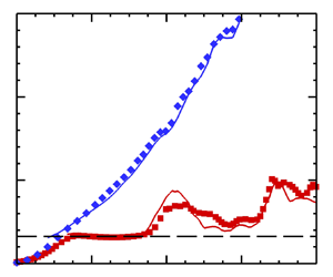
To investigate the bubble RA behaviours in stratified compressible RTI, the bubble velocity  $V_b$ is plotted in figure 1 at different $A_T$ and $Re_p$ for weak ( $Ma=0.1$) and strong ( $Ma=0.7$) stratification strengths. At early time, $V_b$ increases exponentially for all cases and reaches the nonlinearly saturated value $V_t$ predicted by potential flow models at $t\approx 1.5$. After that, the bubble undergoes RA so that $V_b$ is well above $V_t$ except for the cases with $Ma=0.7$ and $A_T=0.1$. However, the effects of $A_T$ on the RA behaviour are quite different for $Ma=0.1$ and $0.7$. For weak stratification ( $Ma=0.1$), increasing the $A_T$ from $0.1$ to $0.9$ while keeping $Re_p$ fixed at $1500$ or 10 000 reduces the maximum value of $V_b$ (see figure 1a), which is consistent with the effect of $A_T$ in unstratified RTI where the RA results from vorticity accumulation inside the bubble (Bian et al. Reference Bian, Aluie, Zhao, Zhang and Livescu2020). The effect of $A_T$ is attributed to the fact that the sites of vortex generation around the sinking spike drift further away from the bubble tip at higher $A_T$, corresponding to a longer travel distance so that vortices obtain an attenuated dissipation before entering the bubble tip region for a fixed $Re_p$ (Bian et al. Reference Bian, Aluie, Zhao, Zhang and Livescu2020). Unlike the effect of $A_T$ on the bubble RA behaviours at $Ma=0.1$, for strong stratification ( $Ma=0.7$), it is clearly seen in figure 1(b) that the bubble accelerates more robustly at higher $A_T$ and decreasing $A_T$ from $0.9$ to $0.1$ suppresses the bubble front development. In particular, at low $A_T$ (e.g. $A_T=0.1$), $V_b$ starts to decrease after reaching the saturated value.

Figure 1. The bubble velocity  $V_b$ versus time for (a) weak ( $Ma=0.1$) and (b) strong ( $Ma=0.7$) stratification strengths. The solid and dashed lines in each panel represent the bubble velocities with $Re_p=10\,000$ and $Re_p=1500$, respectively. The horizontal black long dashed line in each panel represents the bubble saturated velocity $V_t$ predicted in potential flow models.
These interesting behaviours of the bubble at high  $Ma$ can be explained by examining the balance between the buoyancy and drag forces via the modified buoyancy-drag model (BDM) proposed in our previous study (Fu et al. Reference Fu, Zhao, Xu, Wang, Liu, Wan and Lu2022). Note that, for the unstratified RTI, balance is realised for the buoyancy and drag forces resulting in a saturated bubble velocity at the potential stage, for example, at the critical moment $t\approx 1.5$ when $h_b\approx 0.2\lambda$ (Wei & Livescu Reference Wei and Livescu2012). Therefore, the variations of the buoyancy and drag forces estimated by the modified BDM with respect to their unstratified counterparts are used to account for the bubble velocity characteristics. As indicated in figure 2, as the bubble height grows at high $Ma=0.7$, the density difference at the bubble tip decreases corresponding to a decrease in the buoyancy driving the bubble compared with the unstratified counterparts; this situation also happens to the drag force due to the decrease of the heavy fluid density in front of the bubble. For example, in the high- $Ma$ stratified RTI of $A_T=0.9$ at $t\approx 1.5$, the modified BDM estimates a decrease extent of $7.47\,\%$ in the buoyancy and of $10.52\,\%$ in the drag compared with its unstratified counterpart; in the case of $A_T=0.1$, the decrease extent is estimated as $7.55\,\%$ for the buoyancy and $6.27\,\%$ for the drag. Accordingly, the growing bubble obtains a late-time robust acceleration at high $A_T=0.9$ whereas there is a deceleration at low $A_T=0.1$. Thus, decreasing $A_T$ from 0.9 to 0.1 suppresses the bubble front development, as observed in figure 1(b).

Figure 2. The density profiles along the vertical lines across the bubble tip ( $x=0$) with $Re_p=10\,000$ for (a) $Ma=0.1,A_T=0.9$, (b) $Ma=0.1,A_T=0.1$, (c) $Ma=0.7,A_T=0.9$ and (d) $Ma=0.7,A_T=0.1$. The circle marked on the density profile denotes the vertical position of the bubble tip and the square represents the position of the spike tip at each moment.
Figure 1 also presents a striking dependence of bubble RA behaviours on  $Re_p$ at $Ma=0.1$ and $0.7$. For weak stratification ( $Ma=0.1$), there are two different trends at $A_T=0.1$ for the $V_b$ development when $Re_p=1500$ and 10 000. Specifically, for $A_T=0.1$ in figure 1(a), $V_b$ of $Re_p=1500$ starts to decay after accelerating to twice the saturated velocity, whereas $V_b$ of $Re_p=10\,000$ undergoes a further RA at $t\approx 6$. In addition, figure 1(a) shows a clear trend of more intense fluctuations in $V_b$ for $Re=10\,000$ with respect to $Re_p=1500$ at a fixed $A_T$. This significant dependence of RA behaviours on $Re_p$ also appears in unstratified RTI, and Bian et al. (Reference Bian, Aluie, Zhao, Zhang and Livescu2020) attributes it to less vorticity dissipation at higher $Re_p$ which leads to more vortices accumulating inside the bubble tip resulting in higher vorticity and, in turn, $V_b$ fluctuating in time. In contrast to the great $V_b$ dependence on $Re_p$ at $Ma=0.1$, the $V_b$ values are almost the same in the cases of strong stratification for $Re_p=1500$ and 10 000 (see figure 1b) at a fixed $A_T$, indicating a weak influence of $Re_p$ on $V_b$.
To further elucidate the RA behaviours in stratified compressible RTI, the late-time behaviour of the bubble is classified into three phases in figure 3 according to Bian et al. (Reference Bian, Aluie, Zhao, Zhang and Livescu2020): robust RA, transient RA and non-RA. A robust RA phase denotes that the bubble re-accelerates robustly at late times (e.g.  $Ma=0.1$, $A_T=0.1$ with $Re_p=10\,000$ and $Ma=0.7$, $A_T=0.9$ with $Re_p=1500$ or 10 000); in the transient RA phase, a bubble re-accelerates transiently but then decelerates (e.g. $Ma=0.1$, $A_T=0.1$ with $Re_p=1500$ and $Ma=0.7$, $A_T=0.5$ with $Re_p=1500$ or 10 000); in the non-RA phase, bubble velocity starts to decay before reaching the saturated value (e.g. $Ma=0.7$, $A_T=0.1$ with $Re_p=1500$ or 10 000). Figure 3(a) summarises the following findings in a phase diagram in the ( $Ma$,
$Ma$,  $A_T$) space with $Re_p=10\,000$. (1) For $Ma=0.1$, the late-time bubble is in the robust RA phase at small $A_T\leqslant 0.3$ and becomes the transient RA phase as $A_T$ is increased to a larger value. (2) When $Ma=0.2$, the late-time bubble is in the robust RA phase at large $A_T\geqslant 0.7$. (3) For $0.3\leqslant M a\leqslant 0.4$, increasing $A_T$ at a constant $Re_p$ leads to a phase change for the late-time bubble from transient RA to robust RA. (4) For higher $Ma\geqslant 0.5$, the late-time bubble at low $A=0.1$ is in the non-RA phase. Increasing $A_T$ changes the bubble phase from non-RA to transient RA and finally to robust RA. For comparison, figure 3(b) presents the $Ma$-
$Ma$- $A_T$ phase diagram illustrating the bubble RA with $Re_p=1500$. In contrast to the cases of $Re_p=10\,000$, the bubble phase of $Re_p=1500$ changes from robust RA to transient RA at small $Ma$ and $A_T$, but unaltered at high $Ma\geqslant 0.4$. The effects of $A_T$ and $Re_p$ on the bubble RA behaviour at strong stratification differs from those at weak stratification, indicating that a novel mechanism coupling vorticity accumulation and flow compressibility sets in the later-time bubble RA for the stratified compressible RTI at high $Ma$.
$Ma$.

Figure 3. Phase diagram of  $Ma$–
$Ma$– $A_T$ illustrating the bubble RA with (a) $Re_p=10\,000$ and (b) $Re_p=1500$. Red and blue symbols indicate that the bubble RA mechanism is dominated by vorticity accumulation and flow compressibility, respectively.
4. Bubble RA model
The bubble RA in quasi-incompressible RTI is driven by vorticity accumulation inside the bubble based on some studies (Ramaprabhu et al. Reference Ramaprabhu, Dimonte, Young, Calder and Fryxell2006, Reference Ramaprabhu, Dimonte, Woodward, Fryer, Rockefeller, Muthuraman, Lin and Jayaraj2012; Hu et al. Reference Hu, Zhang, Tian, He and Li2019; Bian et al. Reference Bian, Aluie, Zhao, Zhang and Livescu2020). For stratified compressible RTI, our most recent work shows that drag reduction on the bubble caused by stratification leads to the compression of the heavy fluid in front of the bubble, namely, the increased flow compressibility becomes more important to enhance the bubble growth (Fu et al. Reference Fu, Zhao, Xu, Wang, Liu, Wan and Lu2022). Here, to clarify the role that flow compressibility plays in the RA mechanism, we employ the velocity Helmholtz decomposition (Wang et al. Reference Wang, Yang, Shi, Xiao, He and Chen2013), i.e.
 \begin{equation} u_i=u_i^s+u_i^c, \end{equation}
where  $(u_1^s,u_2^s)=(u^s,v^s)$ and $(u_1^c,u_2^c)=(u^c,v^c)$ are the solenoidal and compressive (irrotational) components, respectively. The clear flow physics are indicated by the contour plots of $v^c$ and $v^s$ with $Re_p=10\,000$ for the case $Ma=0.1$, $A_T=0.1$ (figure 4a) and $Ma=0.7$, $A_T=0.9$ (figure 4c) at $t=4$ when the bubble is in the robust RA phase. For weak stratification of $A_T=0.1$, it is clearly seen in figure 4(a) that abundant vortices generated at the spike's interface penetrate into the bubble tip and $v^s$ is dominant to $v$ inside the bubble (see figure 4b). The vertical compressive velocity $v^c$ in figure 4(a) is almost zero over the whole field, indicating that the effects of flow compressibility can be ignored for the case with $Ma=0.1$ and $A_T=0.1$. However, for strong stratification of $A_T=0.9$, $v^c$ is significant across the bubble tip (see figure 4d) caused by the compression of the rising bubble on the heavy fluid in its front (Fu et al. Reference Fu, Zhao, Xu, Wang, Liu, Wan and Lu2022). It is also noted in figure 4(c) that $v^s$ near the bubble tip is negligible compared with $v^c$, because it is difficult at high $A_T$ for the vortices generated at the spike interface to be convected into the bubble front (Bian et al. Reference Bian, Aluie, Zhao, Zhang and Livescu2020). In addition, figure 4(c) presents that $v^c$ near the bubble tip is almost uniform along the horizontal direction.

Figure 4. (a,c) Contour plots of compressive ( $v^c$, left half) and the solenoidal ( $v^s$, right half) components of vertical velocity $v$ and (b,d) profiles of $v$,
$v$,  $v^c$, and $v^s$ along the vertical lines across the bubble ( $x=0$, denoted by the solid lines) and spike ( $x=0.5$, denoted by dashed lines) tips with $Re_p=10\,000$ for (a,b) $A_T=0.1,Ma=0.1$ and (c,d) $A_T=0.9, Ma=0.7$ at $t=4$ when the bubble is in the robust RA phase. The dark lines in panels (a,c) represent the heavy/light fluid interface where $Y_h=0.5$.
The analysis shows that both vorticity accumulation and flow compressibility work as the mechanisms driving the bubble RA in stratified compressible RTI. In order to determine which of these two mechanisms is dominant, based on the fact that the bubble velocity ( $V_b={\rm d}h_b/{\rm d}t$) is equal to the vertical velocity of fluid at the bubble tip ( $v_b$) (Goncharov Reference Goncharov2002), $V_b$ can be decomposed into $V_b^s$ and $V_b^c$ by setting $V_b^s=v_b^s$ and $V_b^c=v_b^c$. Here, $v_b^s$ and $v_b^c$ denote the solenoidal and compressive components of $v_b$, which are related to the vorticity and the dilatation, respectively. Furthermore, the values of $\langle V_b^s-V_b^s|_{t_s}\rangle$ and $\langle V_b^c-V_b^c|_{t_s}\rangle$ correspond to the contributions of vorticity accumulation and flow compressibility at the bubble RA stage, respectively. Here, $\langle \cdot \rangle$ denotes the time average from the moment ( $t_s$) when the bubble velocity reaches the saturation value of the unstratified RTI to the end of simulation, $V_b^s|_{t_s}$ and $V_b^c|_{t_s}$ denote the values of $V_b^s$ and $V_b^c$ at time $t_s$, respectively. It is clearly shown in figure 3 that flow compressibility dominates the bubble RA behaviour in the cases of strong stratification and high $A_T$ whereas vorticity accumulation dominates at small $Ma$ and small $A_T$. Therefore, the $A_T$ effect and $Re_p$ effect at strong stratification are different from those at weak stratification (see figure 1).
Next, we attempt to propose a model to describe the bubble RA behaviours in stratified compressible RTI, quantifying the effects of vorticity accumulation and flow compressibility. As different mechanisms,  $V_b^s$ and $V_b^c$ need to be modelled separately. Bian et al. (Reference Bian, Aluie, Zhao, Zhang and Livescu2020) modified the RA model (Betti & Sanz Reference Betti and Sanz2006) by adding an efficiency factor $\eta =0.45$ to the vorticity term to account for the attenuation of vortices as they travel through the bubble tip region and predict well the bubble RA behaviours driven by vorticity accumulation. In that, $V_b^s$ in stratified compressible RTI can also be modelled as
 \begin{equation} V_b^{\omega}=\sqrt{\frac{g (1-r_d)}{C_d k} + \eta r_d \frac{\omega_0^2}{4k^2}}.\end{equation}
Here,  $C_d=3$ for two dimensions, $\omega _0 = {{\int _{V} \rho |\omega |\,{\rm d}V }/{\int _{V} \rho \,{\rm d}V}}$, $\omega =\partial v/\partial x-\partial u/\partial y$ and $V$ is the volume inside the bubble from the bubble front to a vertical distance of $2/k$ below ( $k$ is the wavenumber). Here $r_d=\rho _l'/\rho _h'$ is the density ratio where $\rho _h'$ is the maximum density at the bubble vertex and $\rho _l'$ is average density in the volume $V$ (Betti & Sanz Reference Betti and Sanz2006). It is shown in figure 5(a,d,g) that the model $V_b^{\omega }$ agrees well with $V_b^s$ evaluated from DNS. Note that the $V_b^{\omega }$ model can also predict the suppression effects at small $A_T$ caused by the stratification on the bubble growth (e.g. the case at $A_T=0.1$ and $Ma=0.7$).

Figure 5. Values of  $V_b^s$, $V_b^c$ and $V_b$ obtained from the DNS (symbols) and $V_b^{\omega }$, $V_b^{\theta }$ and $V_b^{\omega, \theta }$ calculated by the models (lines) with $Re_p=10\,000$ versus time for (a–c) $Ma=0.1$, (d–f) $Ma=0.4$ and (g–i) $Ma=0.7$. The horizontal black long dashed line in each panel represents the bubble saturated velocity $V_t$ predicted in potential flow models.
For  $V_b^c$ caused by flow compressibility, the dilatation $\theta$ (i.e. divergence of velocity) has been introduced naturally to the model. According to the Helmholtz decomposition, $\theta = \partial u^c_i / \partial x_i$. By employing Green's formula, integrating $\theta$ yields
 \begin{equation} \displaystyle\mathop{\iint}\nolimits_S \theta \,{\rm d} S=\oint_{\partial S} u^c\,{\rm d} y - v^c\,{\rm d} x. \end{equation}
Here,  $S$ is the integral region above the bubble tip ( $y_b=h_b$) where the heavy fluid is compressed by the bubble, i.e. $S=[0,L_x] \times [y_b,y_{+\infty }]$, where $y_{+\infty }$ is referred to as any location far away from the bubble tip where the fluid keeps the hydrostatic equilibrium and thus the fluid velocity is zero. Therefore, the upper boundary of the computational domain with the fluid velocity being almost zero is used as $y_{+\infty }$. Considering $v^c$ at the height of the bubble tip is almost uniform along the periodic $x$-direction and thus can be approximated as $V_b^c$, the right-hand side of (4.3) is approximated as $-L_xV_b^c$. The left-hand side of (4.3) can be expressed by the spatial average dilatation $\bar {\theta }$ in the region $S$, i.e. $\iint _S \theta \,{\rm d} S=hL_x\bar {\theta }$, where $h=y_{+\infty }-y_b$ is the height of the region $S$. Thus, $V_b^c$ is modelled as
 \begin{equation} V_b^{\theta}={-}h\bar{\theta}.\end{equation}
Figure 5(b,e,h) shows excellent agreement between the model prediction ( $V_b^{\theta }$) with the DNS result ( $V_b^c$). Furthermore, for a given $A_T$, $V_b^\theta$ at the RA stage obtains a remarkable increase as $Ma$ is increased, resulting from that the stronger density stratification at higher $Ma$ leads to a greater reduction in drag acting on the bubble and in turn more intense compression of the bubble on the heavy fluid ahead.
By summing the equations (4.2) and (4.4), a novel model describing the bubble RA behaviours in stratified compressible RTI can be obtained as
 \begin{equation} V_b^{\omega , \theta}=\sqrt{\frac{g (1-r_d)}{C_d k} + \eta r_d \frac{\omega_0^2}{4k^2}} - h\bar{\theta}. \end{equation}
Figure 5(c, f,i) shows that the model (4.5) captures well the bubble velocity development after the potential stage ( $t\approx 1.5$). This agreement further supports the interpretation that both vorticity accumulation inside the bubble tip and flow compressibility are responsible for the bubble RA.
Although our discussion is based on 2-D simulations, the uncovered mechanisms of bubble RA are straightforwardly applicable to the three-dimensional (3-D) compressible RTI, as the model (4.5) can also be extended to the 3-D flows by modelling the  $V_b^s$ and $V_b^c$ separately. For 3-D RTI $V_b^s$ can be modelled as the same form of (4.2) in which $C_d=1$ (Betti & Sanz Reference Betti and Sanz2006; Yan et al. Reference Yan, Betti, Sanz, Aluie, Liu and Frank2016). On the other hand, $V_b^c$ related to flow compressibility for 3-D situation can be modelled by
Here, Gauss's law is employed along with the Helmholtz decomposition,  $\theta = \partial u^c_i / \partial x_i$, and the gravity direction is fixed along the $y$-direction. We use ${V'}$ to denote the integral volume above the bubble tip where the heavy fluid is compressed by the bubble, i.e. ${V'}=[0,L_x] \times [y_b,y_{+\infty }] \times [0,L_z]$. Considering that $v^c$ at the height of the bubble tip is almost uniform along the periodic $x$- and $z$-directions and, thus, can be approximated as $V_b^c$, the right-hand side of (
) is approximated as  $-L_xL_zV_b^c$. Similar to the 2-D case, the left-hand side of (
) is expressed by the spatially averaged dilatation  $\bar {\theta }$ in the volume ${V'}$, i.e. $\iiint _{V'} \theta \,{\rm d} V=hL_xL_z\bar {\theta }$, where $h=y_{+\infty }-y_b$ is the height of the volume ${V'}$. Thus, $V_b^c$ is also modelled as $V_b^{\theta }= -h\bar {\theta }$. To this end, the model $V^{\omega, \theta }_b$ is extended to the 3-D compressible RTI and has the same form as its 2-D counterpart, i.e. (4.5).
To verify that the model  $V^{\omega, \theta }_b$ is applicable to the 3-D case, the 3-D stratified compressible RTI for $Re_p=1500$ has been simulated in three typical cases: (1) $Ma=0.1$, $A_T=0.1$ corresponding to the bubble RA determined by vorticity accumulation; (2) $Ma=0.7$, $A_T=0.9$ corresponding to the bubble RA dominated by flow compressibility; (3) $Ma=0.7$, $A_T=0.1$ corresponding to the bubble deceleration. Here, the computational domain is set as $L_x\times L_y\times L_z=[0,1]\times [-5,5]\times [0,1]$ and the uniform cubic mesh size $\varDelta =0.01$ is used. Considering that the horizontal component of vorticity accelerates the bubble growth (Yan et al. Reference Yan, Betti, Sanz, Aluie, Liu and Frank2016), the vorticity term in (4.5) is calculated as $\omega _0=\int _V\rho \sqrt {\omega _x^2+\omega _z^2}\,{\rm d}V/\int _V\rho \,{\rm d}V$ for 3-D cases, where $\omega _x$ and $\omega _z$ are the $x$- and $z$-directions components of vorticity, respectively. The efficiency factor of the vorticity term in (4.5) is selected as $\eta =0.85$ for 3-D cases. It is clearly seen in figure 6 that $V_b^\omega$ and $V_b^\theta$ agree well with $V_b^s$ and $V_b^c$ evaluated from the simulations, respectively, and the current model $V_b^{\omega,\theta }$ also captures well the 3-D bubble velocity development after the potential stage ( $t \approx 2.0$). This agreement further supports that the two mechanisms accounting for the bubble RA are applicable to the 3-D compressible RTI. To this point, the model $V^{\omega, \theta }_b$ provides a theoretical basis for the systematic study of nonlinear behaviours for 3-D stratified compressible RTI in the future.

Figure 6. Values of  $V_b^s$, $V_b^c$ and $V_b$ obtained from the simulations (symbols) and $V_b^{\omega }$, $V_b^{\theta }$ and $V_b^{\omega, \theta }$ calculated by the 3-D models (lines) with $Re_p=1500$ versus time for three typical cases. The horizontal black long dashed line in each panel represents the 3-D bubble saturated velocity predicted in potential flow models.
5. Concluding remarks
In summary, highly nonlinear bubble evolution occurring in a single-mode stratified compressible RTI has been reported via DNS. Specifically, the bubble RA behaviours are found except in the cases with high  $Ma$ quantifying the isothermal stratification and small $A_T$. For small $Ma$, both decreasing $A_T$ and increasing $Re_p$ make the bubble RA more intense, which is the same as that in the quasi-incompressible RTI with uniform background density. However, it is interesting that for high $Ma$, increasing $A_T$ enhances the bubble development and $Re_p$ has little effect on the bubble RA behaviour. This flow phenomenon is ascribed to flow compressibility which results from the background stratification and sets in the bubble RA as a novel mechanism coupled with vorticity accumulation inside the bubble for stratified compressible RTI. Inspired by the aforementioned flow physics, a novel model has been proposed via the introduction of the dilatation to account for the effects of flow compressibility, into the classical RA model that only takes into account vorticity accumulation. This improved model performs reliably to capture the bubble velocity development after the potential stage in the stratified compressible RTI.
Note that the current novel bubble RA model which inherits the illuminating idea of the Betti–Sanz model (Betti & Sanz Reference Betti and Sanz2006), still requires the simulation and thus is not predictive. Nevertheless, it succeeds in quantifying the importance of flow compressibility and vorticity accumulation to the bubble growth in stratified compressible RTI, presenting a functional description of bubble velocity. One should keep in mind that, due to the challenging complexity and high nonlinearity of the late-time bubble behaviour in compressible RTI, a predictive model to describe the bubble RA is still lacking. To this point, we believe that the bubble RA mechanism quantified in this extended model would be instructive to the research community working to develop a predictive model for the nonlinear bubble behaviour.
Acknowledgements
The authors are very grateful to Professor R. Yan at USTC for helpful discussions and Dr Y.-S. Zhang at the Institute of Applied Physics and Computational Mathematics for technical support.
Funding
This work was supported by the National Natural Science Foundation of China (Nos. 11621202, 12202436 and 92052301), LCP Fund for Young Scholar (No. 6142A05QN22002) and the Fundamental Research Funds for the Central Universities.
Declaration of interests
The authors report no conflicts of interest.


