


Introduction
For most of the Antarctic ice sheet (AIS), the near-surface climate is too cold to allow for widespread or continuous summer melting, such as occurs in the lower ablation zone of the Greenland ice sheet (Bell and others, Reference Bell, Banwell, Trusel and Kingslake2018). Therefore, in most of Antarctica, surface melting is an intermittent process, associated with warm and moist air advection (Scott and others, Reference Scott, Nicolas, Bromwich, Norris and Lubin2019). An exception is the Antarctic Peninsula (AP), where the relatively mild summer climate allows for more extensive melt episodes (Kuipers Munneke and others, Reference Kuipers Munneke, Picard, Van den Broeke, Lenaerts and Van Meijgaard2012a; Barrand and others, Reference Barrand2013; Luckman and others, Reference Luckman2014), while on the east side of the AP föhn events cause episodic surface melt throughout the year (Kuipers Munneke and others, Reference Kuipers Munneke2018; Wiesenekker and others, Reference Wiesenekker, Kuipers Munneke, Van den Broeke and Smeets2018). Most meltwater refreezes in the cold firn, and runoff currently represents a negligible contribution to AIS mass balance (Van Wessem and others, Reference Van Wessem2018). In spite of this, meltwater lakes are widespread on the AIS (Kingslake and others, Reference Kingslake, Ely, Das and Bell2017; Bell and others, Reference Bell2017; Stokes and others, Reference Stokes, Sanderson, Miles, Jamieson and Leeson2019), and have the potential to influence its dynamical evolution. On ice shelves in the eastern AP, firn saturation and meltwater ponding have been associated with ice-shelf hydrofracturing (Banwell and others, Reference Banwell, MacAyeal and Sergienko2013; Kuipers Munneke and others, Reference Kuipers Munneke, Ligtenberg, Van den Broeke and Vaughan2014). Ice shelves buttress the glaciers that feed them; therefore, ice-shelf disintegration causes glacier acceleration (Scambos and others, Reference Scambos, Bohlander, Shuman and Skvarca2004), which leads in turn to grounded ice loss and sea-level rise. Trusel and others (Reference Trusel2015) suggest a melt rate threshold for ice-shelf viability of 725 mm w.e. a−1, but with considerable uncertainty associated with firn conditions, basal melt rates and ice-shelf stress regimes. As ice shelves are present along ~74% of the margins of the AIS (Bindschadler and others, 2011), the developments in the AP could serve as an analogue for future ice-shelf disintegration and ice-sheet destabilisation elsewhere in Antarctica when the climate continues to warm, with different roles for local and large-scale atmospheric circulation and ice dynamics (Nicolas and Bromwich, Reference Nicolas and Bromwich2014; Fürst and others, Reference Fürst2016; Reese and others, Reference Reese, Gudmundsson, Levermann and Winkelmann2018). That is why a robust quantification and understanding of contemporary Antarctic surface melt is essential for improving future predictions of AIS mass loss and sea level rise (Trusel and others, Reference Trusel2015; DeConto and Pollard, Reference DeConto and Pollard2016).
Nevertheless, very few studies exist that directly and robustly quantify in situ surface melt rates in Antarctica. The main reason is that this requires accurate measurements, not only of near-surface climate variables (pressure, wind speed, temperature and humidity) but also incoming and outgoing shortwave and longwave radiation fluxes. Only then can the surface energy balance (SEB) be closed and the energy available for surface melt be quantified (e.g. Reijmer and Oerlemans, Reference Reijmer and Oerlemans2002; Van den Broeke and others, Reference Van den Broeke, Reijmer, Van As and Boot2006; Kuipers Munneke and others, Reference Kuipers Munneke, Van den Broeke, King, Gray and Reijmer2012b). Apart from the remoteness and the harsh climate, in situ observations in Antarctica are also hindered by accumulating snow, which buries the instruments if they are not regularly raised. Hence, very few Automatic Weather Stations (AWSs) or even staffed meteorological stations on the ice sheet are equipped with radiation sensors (Kuipers Munneke and others, Reference Kuipers Munneke, Ligtenberg, Van den Broeke and Vaughan2014, Reference Kuipers Munneke2018). The prime long-term (1981–present) site is Neumayer station, located on the Ekström Ice Shelf in Dronning Maud Land (DML), which is part of the Baseline Surface Radiation Network and therefore also provides high-quality radiation measurements. Furthermore, it has the added benefit of being situated on the ice shelf, rather than on ice-free rock with very different surface characteristics (Van den Broeke and others, Reference Van den Broeke, Reijmer, Van As, Van de Wal and Oerlemans2005, Reference Van den Broeke, König-Langlo, Picard, Kuipers Munneke and Lenaerts2010b; König-Langlo and Loose, Reference König-Langlo and Loose2007; Jakobs and others, Reference Jakobs, Reijmer, Kuipers Munneke, König-Langlo and Van den Broeke2019).
To circumvent the scarcity of suitable in situ observations, alternative methods have been developed to assess Antarctic surface melt rates. Temperature–index models rely solely on air temperature records and assume melt to occur when air temperature exceeds 0°C while adopting an index that couples the air temperature to surface melt rate. This method has proven valuable to obtain longer-term regional estimates for Antarctic surface melt patterns (Van den Broeke, Reference Van den Broeke2005; Barrand and others, Reference Barrand2013; Leeson and others, Reference Leeson2017), but lacks a physical basis and properly constrained parameters (Wake and Marshall, Reference Wake and Marshall2015); for instance, it does not explicitly resolve the snowmelt–albedo feedback, which has the potential to enhance melt rates threefold in Antarctic regions with intermittent melt (Jakobs and others, Reference Jakobs, Reijmer, Kuipers Munneke, König-Langlo and Van den Broeke2019). Remote sensing provides a valuable tool for the direct, continent-wide observation of surface melt by measuring surface brightness temperatures (Picard and others, Reference Picard, Fily and Gallée2007) and by the attenuation of radar waves in the presence of liquid water in the near-surface snow (Trusel and others, Reference Trusel, Frey and Das2012). By correlating satellite signal attenuation to in situ surface melt, continent-wide maps of summer melt totals can be obtained (Trusel and others, Reference Trusel, Frey, Das, Kuipers Munneke and Van den Broeke2013). Finally, surface melt rates can be modelled using (regional) climate models (King and others, Reference King2015; Kuipers Munneke and others, Reference Kuipers Munneke2017; Van Wessem and others, Reference Van Wessem2018; Donat-Magnin and others, Reference Donat-Magnin2019). These models generally perform adequately, but suffer from climate biases and limited resolution that smoothens the topography, especially in topographically steep regions such as the AP and the relatively steep escarpment zone in DML, East Antarctica. This smoothing results in biases in temperature, wind speed and surface melt (Van Wessem and others, Reference Van Wessem2014a).
All of these methods depend on in situ observations of melt rates for calibration (temperature–index models, satellite melt rate), validation (satellite melt detection) or evaluation (climate models). That is why building a benchmark dataset of consistently derived in situ Antarctic melt rate observations is crucial. As of today, most studies that have explicitly quantified the SEB and melt rate in Antarctica were restricted to a single location, for example the Larsen C Ice Shelf in the AP (Kuipers Munneke and others, Reference Kuipers Munneke, Van den Broeke, King, Gray and Reijmer2012b; King and others, Reference King2015, Reference King2017), Berkner Island (Reijmer and others, Reference Reijmer, Greuell and Oerlemans1999) or glaciers situated on islands close to the AP (e.g. Bintanja, Reference Bintanja1995; Jonsell and others, Reference Jonsell, Navarro, Bañón, Lapazaran and Otero2012; Falk and others, Reference Falk, López and Silva-Busso2018). While these studies provide important information about surface melt and its temporal variability, their spatial coverage remains limited.
Here, we present a benchmark dataset of Antarctic surface melt rates and energy balance from one staffed research station (Neumayer) and eight AWSs. All sites are located in the Atlantic sector of Antarctica, ranging from the eastern AP to DML (Fig. 1). Although some individual results from Neumayer and three AWSs have been published before (e.g. Van den Broeke and others, Reference Van den Broeke, König-Langlo, Picard, Kuipers Munneke and Lenaerts2010b; Kuipers Munneke and others, Reference Kuipers Munneke, Van den Broeke, King, Gray and Reijmer2012b, Reference Kuipers Munneke2018; King and others, Reference King2015, Reference King2017; Wiesenekker and others, Reference Wiesenekker, Kuipers Munneke, Van den Broeke and Smeets2018; Jakobs and others, Reference Jakobs, Reijmer, Kuipers Munneke, König-Langlo and Van den Broeke2019), this study expands on previous work by updating the time series, using a single SEB model framework to process all station data and determine uncertainties in a consistent manner. Subsequently, we use the resulting in situ melt data to assess the validity of simplified temperature–index models, evaluate Antarctic surface melt from the regional climate model RACMO2 and validate the QuikSCAT satellite melt product.
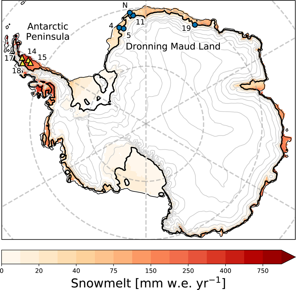
Fig. 1. Locations and identifiers of used automatic weather stations in the AP (yellow triangles) and DML (blue dots). Neumayer station is denoted with an N (blue dot). Background colours represent period-average annual melt amounts (1979–2017) as simulated by the regional atmospheric climate model RACMO2 (Van Wessem and others, Reference Van Wessem2018). The thin black line represents the 10 m height contour (~shelf edge), the thick black line represents the 150 m height contour (~grounding line), grey lines indicate 500 m height intervals.
In the next section, we describe the instruments used on the weather stations and introduce the SEB model. Next, we present the dataset and discuss its main characteristics including annual averages and seasonal and daily variability. We proceed to use the new dataset to calibrate, evaluate and validate alternative Antarctic melt products, followed by conclusions.
Methods
Automatic weather stations
Since 1995, the Institute for Marine and Atmospheric Research of Utrecht University (IMAU) has deployed and maintained 19 AWSs in Antarctica. As of November 2019, four of these AWSs are still operational. The stations have technically evolved from Type 1 (T1) to Type 3 (T3) (Table 1, see also Smeets and others, Reference Smeets2018). Here we only use data of T2 and T3 AWSs as these measure the full radiation balance, that is incoming and reflected broadband shortwave radiation, SW↓ and SW↑, and downward and upward broadband longwave radiation, LW↓ and LW↑. In addition, the AWS measure near-surface air temperature (T), wind speed (WS), wind direction (WD), relative humidity (RH), instrument height (H), air pressure (p) and snow temperature (T sn) at various depths. Specifications of the used sensors are presented in Table 1. The stations sample every 6 min, after which 2-hourly (T2, until January 2001), hourly (T2, from January 2001 onwards) or half-hourly (T3) means are calculated, stored locally and transmitted through the Argos satellite system. The AWSs are powered by lithium batteries, while T3 stations in addition use solar cells. The temperature/humidity and radiation sensors are not ventilated because of energy considerations, which may negatively affect their performance. The magnitude of the resulting error depends on the amount of incoming and reflected solar radiation, the wind speed and the type of radiation shield used (Van den Broeke and others, Reference Van den Broeke, Van As, Reijmer and Van de Wal2004c). Bintanja (Reference Bintanja2000) and Van As and others (Reference Van As, Van den Broeke, Reijmer and Van de Wal2005) show that, based on a comparison with ventilated instruments, the radiation error does not exceed the sensor accuracy listed in Table 1 for the T2 stations.
Table 1. Sensors used on the different types of automatic weather stations
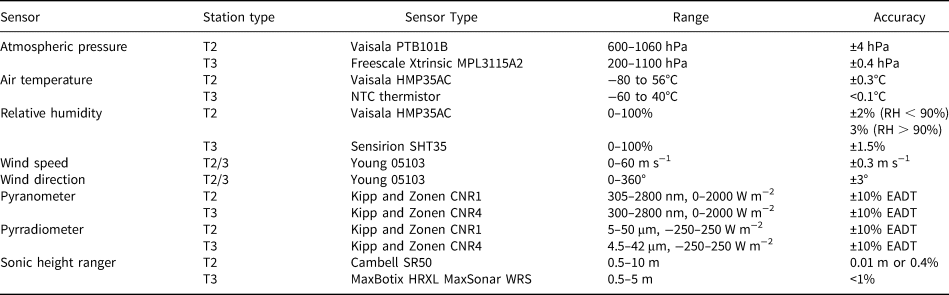
EADT = estimated accuracy for daily totals. For technical details of the observations at Neumayer the reader is referred to König-Langlo and Loose (Reference König-Langlo and Loose2007) and Jakobs and others (Reference Jakobs, Reijmer, Kuipers Munneke, König-Langlo and Van den Broeke2019).
Due to the low temperatures encountered at several sites, some of the sensors are operated outside of their range of operational specifications. This mostly affects the relative humidity and longwave radiation observations. The relative humidity observations are corrected based on the method described by Anderson (Reference Anderson1994) and Van den Broeke and others (Reference Van den Broeke, Reijmer and Van de Wal2004a). The accuracy of the radiation sensors, which are affected by icing/riming, tilt, low sun angles and window heating offset, is discussed in Van den Broeke and others (Reference Van den Broeke, Van As, Reijmer and Van de Wal2004c). They conclude that with an accuracy of 5% for the daily averages, the radiation sensors perform better than their specifications; we follow their methods to check for rime formation. To reduce net shortwave radiation errors on sub-daily time scales, we calculate a 24 h running mean albedo, which is then applied to the reflected shortwave radiation to obtain incoming and net shortwave radiation fluxes. For all variables, erroneous values were removed by automated and manual detection.
We use data of four AWSs on ice shelves in the eastern AP and four in DML, East Antarctica (indicated in Fig. 1). Furthermore, we use data of Neumayer Station, located on Ekström Ice Shelf in DML (König-Langlo, Reference König-Langlo2017) (also indicated in Fig. 1). The Neumayer meteorological observatory is operated by the Alfred Wegener Institute and is part of the Baseline Surface Radiation Network, a global network of artificially ventilated, high-quality radiation observations, with instantaneous individual broadband fluxes more accurate than 5 W m−2 (see König-Langlo and Loose (Reference König-Langlo and Loose2007) for technical specifications and Jakobs and others (Reference Jakobs, Reijmer, Kuipers Munneke, König-Langlo and Van den Broeke2019) for measurement accuracies). The same variables are measured at Neumayer as by the AWS except for the sonic height ranger, which is not present at Neumayer. Instead, height changes are measured at Neumayer by weekly stake measurements.
Table 2 provides station names, locations, altitudes and observation period of the stations used in this study. AWS 4 was located on the flat Riiser-Larsen ice shelf, AWS 5 was located inland of the grounding line in the steep escarpment zone, dominated by katabatic winds (Van den Broeke and others, Reference Van den Broeke1999; Van Wessem and others, Reference Van Wessem2014a). Neumayer is located on Ekström ice shelf, which is prone to low-pressure systems passing north of the station. This results in frequent strong synoptically-forced easterly winds, advecting warm moist air (Herman and others, Reference Herman2013). AWS 11 was located relatively close to Neumayer but on an ice rise; its higher elevation leads to significantly less surface melt. AWS 19 was located close to the grounding line on the Roi Baudouin ice shelf, where föhn winds occur frequently (Lenaerts and others, Reference Lenaerts2017). In the AP, AWS 18 is also prone to frequent föhn events, located close to the grounding line just east of the AP mountain range (Kuipers Munneke and others, Reference Kuipers Munneke2018; Wiesenekker and others, Reference Wiesenekker, Kuipers Munneke, Van den Broeke and Smeets2018). Farther from the grounding line on the flat ice shelf, AWS 14 and 15 are affected much less by föhn winds. AWS 17 was located more to the north on Scar Inlet, the Larsen B remnant. Because of the northerly location, it experienced more melt than AWS 14 and 15.
Table 2. Overview of AWS used in this study: locations, elevations and period of operation (see also Fig. 1)
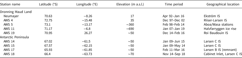
Except for AWS 5 and 11, all stations are located on ice shelves (denoted by IS).
Surface energy balance model
Surface melt energy is calculated by solving the SEB equation:

in which SWnet and LWnet are the net short- and longwave radiation fluxes, Q S and Q L are the turbulent fluxes of sensible and latent heat, Q G the conductive subsurface heat flux, and M the energy available for surface melt respectively. By convention, positive fluxes are directed towards the surface. The turbulent fluxes Q S and Q L are calculated using the flux-profile method between the measurement level and the surface, using Monin–Obukhov similarity theory with the stability functions from Dyer (Reference Dyer1974) for unstable conditions and those from Holtslag and De Bruin (Reference Holtslag and De Bruin1988) for stable conditions. Energy added through liquid precipitation is neglected as rainfall is rare in Antarctica. M is zero when the surface temperature T S is below the freezing point (273.15 K). T S is derived by assuming the energy balance equation to be valid for an infinitesimally thin surface layer (skin layer). To that end, all terms in Eqn (1), apart from SWnet and LW↓, are expressed as a function of T S after which Eqn (1) is solved iteratively for T S so that the SEB is closed. A more detailed description of the model can be found in Reijmer and others (Reference Reijmer, Greuell and Oerlemans1999).
The snowpack is initialised with 70 layers of varying thickness: 1 cm at the top, gradually increasing to 2 m at 25 m. The lowest layer is kept at a constant, prescribed temperature: the annually averaged air temperature. Layer thickness can vary as a result of dry snow densification, meltwater refreezing and mass changes by sublimation or deposition. Meltwater percolation is modelled with the tipping-bucket method (e.g. Ligtenberg and others, Reference Ligtenberg, Kuipers Munneke and Van den Broeke2014), in which meltwater is assumed to percolate downwards instantaneously when a layer has reached its maximum capillary retention, which is parameterised following Schneider and Jansson (Reference Schneider and Jansson2004). Shortwave radiation penetration into the subsurface is calculated using a spectral model from Kuipers Munneke and others (Reference Kuipers Munneke2009), based on Schlatter (Reference Schlatter1972) and Brandt and Warren (Reference Brandt and Warren1993). Temperature and specific humidity are recalculated to 2 m values and wind speed to 10 m values using Monin–Obukhov similarity theory.
For all stations, we use the same constant value for surface momentum roughness length z 0,m of 1.65 mm, following Jakobs and others (Reference Jakobs, Reijmer, Kuipers Munneke, König-Langlo and Van den Broeke2019). Currently, insufficient data are available to make z 0,m time-dependent across the stations in a consistent manner. The surface roughness lengths for moisture and heat are calculated using the expressions of Andreas (Reference Andreas1987). The density of new snow is determined for each station separately by running the model multiple times and minimising the difference between modelled T S and observed T S derived from LW↑. The sensitivity to different choices for z 0,m, new snow density and the inclusion of shortwave radiation penetration are used to estimate the uncertainty in the determined heat fluxes and surface melt rates following the method outlined in Jakobs and others (Reference Jakobs, Reijmer, Kuipers Munneke, König-Langlo and Van den Broeke2019).
Results
Annual means and seasonal cycles
Table 3 lists annual (July–June) totals (snowmelt, sublimation) and mean values of climatological variables and SEB components for the nine sites. Surface melt and sublimation rates are expressed in mm w.e. a−1, which is equal to kg m−2 a−1. Uncertainties in Q S, Q L, Q G, M, snowmelt and sublimation are derived from sensitivity experiments (following Jakobs and others, Reference Jakobs, Reijmer, Kuipers Munneke, König-Langlo and Van den Broeke2019), the other uncertainties are derived from measurement uncertainties (Table 1). The large uncertainty in Q G is a result of taking radiation penetration into account; when it is accounted for, energy that would have been provided to the surface by SW↓ is instead absorbed in the subsurface, which is eventually provided to the surface through Q G.
Table 3. Annual (July–June) values of climatological variables and SEB components for AWS and Neumayer station

The top row indicates whether the station is located in DML or the AP, the third row indicates the period of observation (mm/yy–mm/yy). Uncertainties in Q S, Q L, Q G, M, snowmelt and sublimation are derived from sensitivity experiments (following Jakobs and others, Reference Jakobs, Reijmer, Kuipers Munneke, König-Langlo and Van den Broeke2019), the other uncertainties are derived from measurement uncertainties (Table 1). aThe values of AWS 19 are averages of January–December, as there is no full July–June period available for that station.
The table shows that in general, stations on the eastern AP ice shelves experience typically an order of magnitude more melt than those in DML (Table 3), mainly driven by the difference in annual average net radiation R net (≡ SWnet + LWnet). Although SW↓ is slightly larger in the AP, the higher precipitation amounts increase the surface albedo sufficiently to result in an SWnet similar to what is observed in DML. However, the warmer air on the eastern AP ice shelves increases LW↓, resulting in a larger R net. Subsequently, the larger Q G is a result of refreezing that occurs in the subsurface snow layers. Refreezing raises the subsurface temperature, and keeps it close to the melting point after melt events.
Figure 2 shows the seasonal cycles of monthly average 2 m temperature, specific humidity and 10 m wind speed (top row), the radiation balance (middle row) and the SEB components (bottom row) for AWS 14, 5 and Neumayer. These three locations were selected because of their relatively long observation period, which demonstrates that they represent three distinct climate regions: the eastern AP ice shelves (AWS 14, left column) and for DML an inland and coastal ice-shelf location (AWS 5 and Neumayer, centre and right). The shading in Figure 2 indicates the standard deviations of the monthly means.
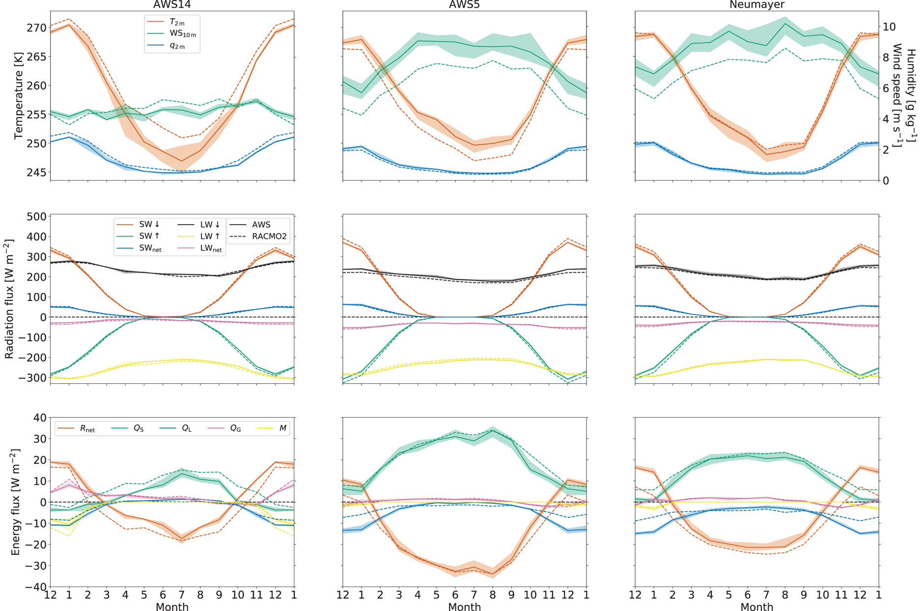
Fig. 2. Seasonal cycles (based on monthly means) of near-surface climate, surface radiation and SEB for AWS 14 (left column), AWS 5 (centre column) and Neumayer (right column). The top panels show the seasonal cycles of 2 m temperature, 10 m wind speed and 2 m specific humidity. The middle panels show the seasonal cycles of upward and downward broadband radiation fluxes, as well as net radiation, and the bottom panels show the seasonal cycles of the SEB components. The shading indicates the standard deviations of the monthly means, based on the available period. December and January are repeated for clarity. Note that these average seasonal cycles are derived using data from different time periods (see Table 2). Outputs for the same period from RACMO2 are shown with dashed lines.
A comparison of the seasonal cycles shows that the highest summer near-surface temperatures are observed in the eastern AP, owing to its more northerly location and exposure to milder maritime air masses. In winter, an interesting result is that AWS 5 and Neumayer, located in DML, experience higher temperatures than the eastern AP. This is caused by stronger wintertime winds at the DML stations, typically 8–10 m s−1 (Van den Broeke and others, Reference Van den Broeke, Reijmer and Van de Wal2004b), compared to 4 m s−1 at AWS 14 (Kuipers Munneke and others, Reference Kuipers Munneke, Van den Broeke, King, Gray and Reijmer2012b; King and others, Reference King2015). The climate of AWS 5, which is located in the escarpment zone, is characterised by katabatic winds that efficiently mix relatively warm air from aloft towards the surface, preventing the formation of a strong surface-based temperature inversion and leading to warming of the surface and near-surface air (Van den Broeke and others, Reference Van den Broeke1999; Van Wessem and others, Reference Van Wessem2014a). At Neumayer, the ice-shelf surface is nearly flat and the resulting katabatic forcing is weak. Here, the higher wind speeds are synoptic in nature, owing to the vicinity of the Atlantic climatological low-pressure system and the associated passage of low-pressure systems to the north of the station (Herman and others, Reference Herman2013). In contrast, AWS 14, also located on a flat ice shelf, is under the influence of cold air that is transported by barrier winds along the spine of the AP (Turner and others, Reference Turner2002); in combination with the relatively low wind speeds, this enables the formation of a strong surface-based temperature inversion, which keeps the climate of the Larsen C Ice Shelf relatively cold in winter (Marshall and King, Reference Marshall and King1998).
The seasonal cycles of the radiation balance (Fig. 2, middle row) show that the minimum in LW↓ is shifted by 1–2 months with respect to SW↓. This is a result of the delay in atmospheric heating in response to slow ambient warming. Net radiation is strongly negative in winter and becomes weakly positive in summer, when in spite of the high surface albedo, absorbed shortwave radiation exceeds the longwave energy loss. Furthermore, as a result of the longer polar night at AWS 5 and Neumayer, the net radiation flux is negative for a longer period than at AWS 14. As stated above, strong winds at AWS 5 and Neumayer enhance Q S, increasing the surface temperature and therewith longwave radiation heat loss (Van den Broeke and others, Reference Van den Broeke, König-Langlo, Picard, Kuipers Munneke and Lenaerts2010b; Jakobs and others, Reference Jakobs, Reijmer, Kuipers Munneke, König-Langlo and Van den Broeke2019). As a result, net radiation at AWS 14 is ~ 10 W m−2 higher in summer and ~ 20 W m−2 higher in winter compared to AWS 5 and Neumayer. The resulting annual mean net radiation flux is almost zero at AWS 14, while it is negative at AWS 5 and Neumayer station. At AWS 17, annual net radiation is positive. The reason for this is twofold: at this site, regular melting decreases surface albedo; owing to the dry climate, the albedo is not frequently reset by fresh snow, thus increasing SWnet. Secondly, the absence of katabatic winds over the flat ice shelf reduces turbulent heating of the surface, limiting longwave heat losses.
The seasonal cycles of all SEB components (Fig. 2, bottom row) show how the differences in surface climate impact surface energy exchange and melt rate. In winter, the high wind speeds at sites AWS 5 and Neumayer result in larger Q S, heating the surface and cooling the atmosphere. This results in additional longwave heat loss, leading to more negative wintertime net radiation (Van den Broeke and others, Reference Van den Broeke, König-Langlo, Picard, Kuipers Munneke and Lenaerts2010b; Jakobs and others, Reference Jakobs, Reijmer, Kuipers Munneke, König-Langlo and Van den Broeke2019). This process is much weaker at AWS 14, where wind speeds are low year-round. In summer at AWS 14, Q S becomes negative, indicating the presence of a (daytime) weakly convective boundary layer (Kuipers Munneke and others, Reference Kuipers Munneke, Van den Broeke, King, Gray and Reijmer2012b; Välisuo and others, Reference Välisuo, Vihma and King2014; King and others, Reference King2015). This is a result of the regular occurrence of melt at this site: it lowers the albedo through wet snow metamorphism, enhancing SWnet and creating negative surface-to-air temperature gradients before melting starts. Surface warming is further enhanced through Q G, which increases significantly in response to warming of the subsurface snow when meltwater refreezes. As melt rates are small at AWS 5 and Neumayer, these effects are weaker there. At all three stations, sublimation (Q L) becomes the largest source of heat loss in summer, when temperatures are sufficiently high to allow for significant surface-to-air specific humidity gradients. At AWS 14, Q L becomes weakly positive in winter, indicating deposition of atmospheric moisture (rime formation) at the surface (Kuipers Munneke and others, Reference Kuipers Munneke, Van den Broeke, King, Gray and Reijmer2012b; Välisuo and others, Reference Välisuo, Vihma and King2014; King and others, Reference King2015).
At all stations, average summer melt energy is typically small, and all SEB components are important in determining its magnitude. To look at the surface melt process in more detail, the following section discusses two case studies, using the full temporal resolution of the dataset.
Two case studies: meteorological drivers of surface melt
The high temporal resolution of the dataset provides an opportunity to investigate surface melt and its drivers more closely. Figure 3 contrasts two melt events in DML (AWS 4 and AWS 5, 27–31 December 1998, left) and on the Larsen C Ice Shelf in the eastern AP (AWS 14 and AWS 18, 7–13 April 2015, right). Note that the AP AWS store data at hourly intervals, while AWS 4 and 5 stored data at a 2-hourly time resolution. AWS 4 was situated on the flat Riiser-Larsen ice shelf and AWS 5 85 km to the ESE, just off the shelf on the grounded ice sheet, but still close to sea level. At this small distance, they experience similar daily cycles. In this relatively cold part of Antarctica, surface melt is intermittent and only occurs during daytime in summer, when insolation is strong enough to raise the surface temperature to the melting point.
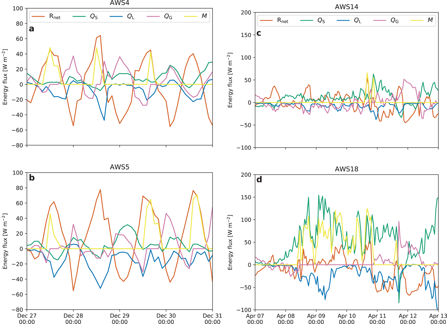
Fig. 3. High-resolution time series of SEB components for AWS 4 and 5 in DML (a and b, 27–31 December 1998, 2 h resolution) and AWS 14 and 18 in the AP (c and d, 7–13 April 2015, 1 h resolution). Note the different vertical axes (a and b compared to c and d).
The selected midsummer period (27–31 December 1998) for AWS 4 and 5 represents a radiation-dominated melt event typical for this location; these daily cycles during the midnight sun are dominated by the net radiation flux being positive when solar radiation is sufficiently large and negative otherwise (Figs 3a, b). Melt occurs when net radiation becomes significantly positive (~50 W m−2) and surface heat sinks (convection, sublimation, subsurface heat conduction) are not strong enough to prevent the surface from reaching the melting point. While both stations experience roughly similar meteorological conditions (Figs 4a–d), melt does not necessarily occur simultaneously at the two locations. For example, on 28 December 1998 melt occurred at AWS 4 but not at AWS 5; on this day, a lower relative humidity and a higher wind speed at AWS 5 enabled stronger sublimation, removing sufficient energy from the surface to prevent surface melt. Note that Rnet was similar at both stations: the higher cloud cover at AWS 4 reduced SWnet but increased LWnet, which effectively cancelled each other.
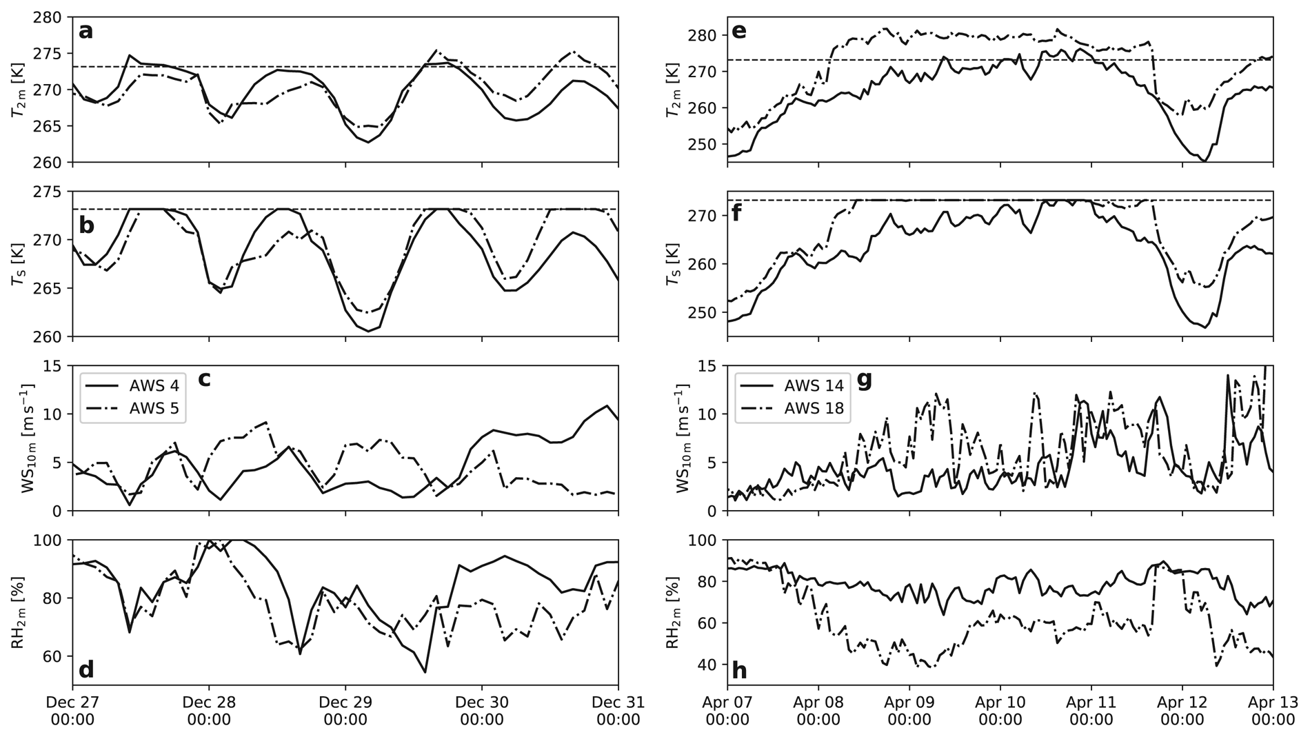
Fig. 4. Time series of T 2 m, T S, WS10 m and RH2 m for AWS 4 and 5 (a–d) and AWS 14 and 18 (e–h) for the same periods as in Figure 3.
Conversely, 2 days later on 30 December 1998, melt occurred at AWS 5 but not at AWS 4, with higher winds and surface cooling by sublimation this time occurring over the ice shelf. We conclude that surface melt in coastal DML is the result of a delicate balance between daytime surface heat sources and heat sinks, and highly sensitive to differences in cloud cover, atmospheric humidity and wind speed.
On the Larsen C Ice Shelf, surface melt also occurs in non-summer months and even during the polar night. Under the influence of strong circumpolar westerlies, föhn winds can develop at the lee (eastern) side of the south-north oriented spine of the AP (Elvidge and others, Reference Elvidge2014; King and others, Reference King2017; Kuipers Munneke and others, Reference Kuipers Munneke2018). During these events, warm and dry air reaches the ice shelf at the foot of the mountains. Turton and others (Reference Turton, Kirchgaessner, Ross and King2018) and Wiesenekker and others (Reference Wiesenekker, Kuipers Munneke, Van den Broeke and Smeets2018) show that föhn events at AWS 18 between November 2014 and December 2016 occur 14% of the time. Even in midwinter, 2 m air temperatures can reach values as high as 10°C, while relative humidity decreases to values below 50%.
AWS 14 and 18 are both located on the Larsen C Ice Shelf in the eastern AP (Fig. 1). AWS 18 is located in Cabinet Inlet, one of the main contributing ice streams of the Larsen C Ice Shelf. AWS 14 is located ~120 km SE of AWS 18, in the middle of the ice shelf and significantly closer to the ice-shelf edge. The spine of the AP causes the occurrence of frequent föhn events at AWS 18 (see e.g. Kuipers Munneke and others, Reference Kuipers Munneke2018; Wiesenekker and others, Reference Wiesenekker, Kuipers Munneke, Van den Broeke and Smeets2018); owing to its location farther from the mountain range, these events are less frequent and less severe at AWS 14 (Turton and others, Reference Turton, Kirchgaessner, Ross and King2018).
Figures 3c, d and 4e–h show the SEB and near-surface climate at AWS 14 and 18, for a 6-day period in April 2015. This event was chosen because of the short overlap between the two stations' observational record, resulting in this event as one of the few events registered by both stations. During this period, a well-developed and long-lasting föhn event was registered at AWS 18, with air temperatures as high as 8.5°C. Surface melt occurred continuously for 60 h, from ~8 April 10:00 until ~10 April 21:00, with a cumulative melted mass of 37 kg m−2. The most important energy source was Q S, reaching peak hourly averaged values of 150 W m−2, aided by the strong winds (11–12 m s−1) and the large temperature gradient between the warm air and the melting surface, which cannot adjust its temperature further upwards. Relative humidity remained as low as 40%, characteristic of föhn winds, leading to significant sublimation with peak hourly average values of 75 W m−2. Without this heat sink, cumulative melt would have been ~44% higher. At AWS 14, owing to its location farther from the AP spine, the föhn effect is significantly less pronounced, with above-freezing air temperatures occurring only towards the end of the episode and cumulative melt totalling 2 kg m−2, 5.4% of that at AWS 18. At AWS 14, the surface temperature remained below freezing for most of the period, with Q G gradually increasing indicating warming of the snowpack by Q S and LWnet, resulting in some surface melt in the final hours of the föhn event. This shows that AP föhn events and the associated melt are spatially highly heterogeneous, and tend to peak in intensity and duration at the foot of the AP mountains.
Evaluation of other surface melt products
Temperature–index models
Temperature–index models are used where radiation observations are not available. By relating surface melt rates to air temperature, an estimate of the former can be determined solely from temperature observations. Typically, these models relate period-total melt amounts to the period-sum of daily T − T c when T > T c, where T c is a freely chosen threshold temperature (usually T c = 0°C) and T is the daily average air temperature (usually at 2 m) (see e.g. Braithwaite, Reference Braithwaite1995; Hock, Reference Hock2003; Van den Broeke and others, Reference Van den Broeke, Bus, Ettema and Smeets2010a). The proportionality constant between daily average T − T c and daily melt amount is the degree day factor (DDF), expressed in mm d−1 K−1. Commonly used values for DDF are in the range 3–8 mm d−1 K−1 (Hock, Reference Hock2003).
Applying this method to all stations with T c = 0°C yields DDFs between 3.3 mm d−1 K−1 (AWS 18) and 55.6 mm d−1 K−1 (AWS 19). The results indicate that DDF is spatially highly variable, with an average value of 26.6 mm d−1 K−1 for DML stations and 5.9 mm d−1 K−1 for eastern AP shelf stations. The very high degree day factors for DML are caused by the intermittent nature of the melt, giving rise to frequent melt days for which average daily temperatures do not exceed 0°C (see also Fig. 4). The variability in the DDF over larger areas was also shown by Van den Broeke and others (Reference Van den Broeke, Bus, Ettema and Smeets2010a) for the Greenland ice sheet. As T is the daily average air temperature, melt days on which daily average T < 0°C are not recognised as melt days, which results in a significant amount (72.5% in terms of total melt) of melt events not being accounted for. This effect is most pronounced in DML, where only 7.6% of the melt days have a daily average T > 0°C, compared to 34.7% on eastern AP ice shelves.
By choosing T c < 0°C, for example when T c is set to − 10°C (following Van den Broeke and others, Reference Van den Broeke, Bus, Ettema and Smeets2010a), all melt events are accounted for; however, the correlation coefficient between predicted and observed daily melt R 2 decreases from 0.36 to 0.33, further lowering the validity of this method. This simple application of the in situ melt rate dataset shows that continent-wide estimates for surface melt cannot be based solely on temperature records and a positive-degree day method.
RACMO2
We compare the in situ surface melt rates to the output of the polar version of the Regional Atmospheric Climate MOdel (current version RACMO2.3p2, from now on RACMO2), which is developed at IMAU in collaboration with the Royal Netherlands Meteorological Institute (KNMI). The model combines the dynamics of the regional model HIRLAM (Undén and others, Reference Undén2002) with the physics parameterisations of ECMWF-IFS (ECMWF, 2008), assuming hydrostatic balance and using 40 vertical levels. It is interactively coupled to a multilayer snow model that calculates melt, refreezing, percolation and runoff of meltwater (Ettema and others, Reference Ettema2010). It furthermore includes a snow albedo scheme based on snow grain size evolution (Kuipers Munneke and others, Reference Kuipers Munneke2011; Van Angelen and others, Reference Van Angelen2012) as well as a drifting snow scheme that simulates the redistribution and sublimation of suspended snow particles (Lenaerts and others, Reference Lenaerts2012). We refer the reader to Van Wessem and others (Reference Van Wessem2014a) and Van Wessem and others (Reference Van Wessem2014b) for more technical details of RACMO2. Here we use the latest gridded 27 km product spanning the period 1979–2017 and covering the entire continent (Fig. 1). The model run is forced at the lateral boundaries and in the upper atmosphere by the ERA-interim reanalysis product (Dee and others, Reference Dee2011). Previous studies have evaluated RACMO2 for temperature, wind speed and SEB components in Antarctica; Van Wessem and others (Reference Van Wessem2018) showed that RACMO2 reproduces surface temperatures and net shortwave radiation with high accuracy (R 2 > 0.9), and turbulent fluxes, net longwave radiation and wind speed with fair accuracy (R 2 > 0.5). The RACMO2 melt product has not been compared to in situ melt data but only to QuikSCAT data, which showed a correlation of R 2 = 0.81 and a bias of −15 Gt a−1 for the entire AIS (~13% of average annual snowmelt) (Van Wessem and others, Reference Van Wessem2018). Furthermore, RACMO2 has been evaluated in terms of SEB components (King and others, Reference King2015) and surface mass balance (Kuipers Munneke and others, Reference Kuipers Munneke2017).
Here, we compare the RACMO2 surface melt rates to the in situ melt rate dataset (Fig. 5). The RACMO2 error bars are empirically determined by calculating the relative deviation from each observation and taking the average; this average relative deviation is then imposed on each model melt point. The errors of the in situ melt values are derived from a parameter uncertainty study with the SEB model (similar to Jakobs and others, Reference Jakobs, Reijmer, Kuipers Munneke, König-Langlo and Van den Broeke2019). The result that deviates most from the baseline run is assumed to represent the uncertainty. Figure 5 presents annual (July–June) surface melt rates for (a) all stations and (b) DML stations only, and shows good correlation (R 2 = 0.83). On average RACMO2 somewhat underestimates melt (bias = −7.3 mm w.e. a−1). When both regions are considered separately the correlation weakens, with R 2 = 0.59 for stations located on the ice shelves in the eastern AP, and R 2 = 0.51 for stations in DML.
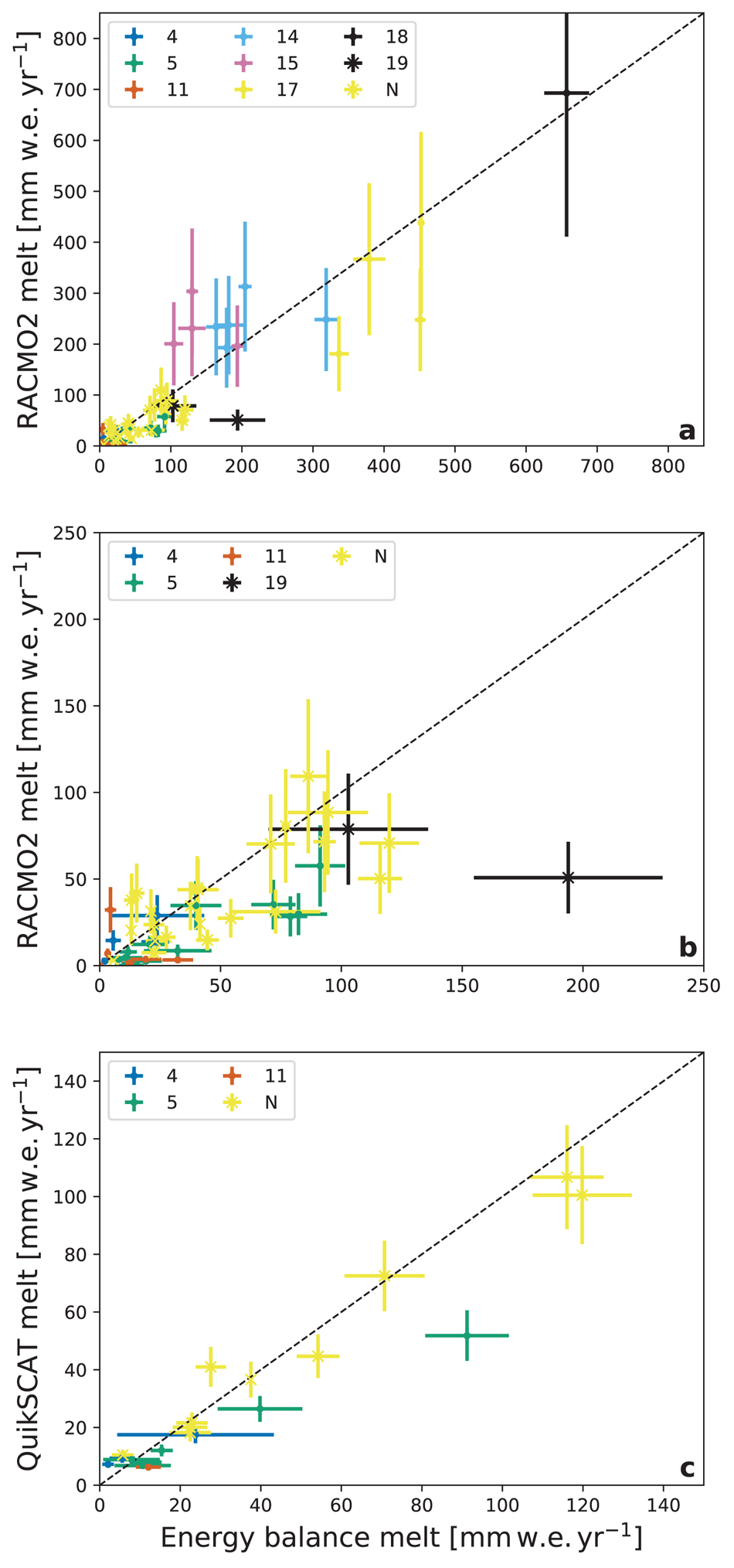
Fig. 5. In situ versus (a, b) RACMO2-modelled and (c) QuikSCAT-derived yearly (July–June) melt. AWSs are indicated by station numbers and Neumayer by N. (a) shows all stations and (b) focuses on DML stations for clarity. Correlation coefficients are (a) 0.83, (b) 0.51 and (c) 0.92. The error bars for RACMO2 (a, b) and QuikSCAT (c) are empirically determined by calculating the relative deviation from each observation and taking the average; this average relative deviation is then imposed on each model melt point. The errors of the in situ melt values are derived from a parameter uncertainty study with the SEB model (similar to Jakobs and others, Reference Jakobs, Reijmer, Kuipers Munneke, König-Langlo and Van den Broeke2019).
Figure 6 presents time series of annual melt (1979–2017) from QuikSCAT (green), discussed in the next section, RACMO2 (blue) and the in situ melt rates (dark orange) for the nine observational sites. The shading indicates the uncertainty based on the SEB-model parameter uncertainty tests. The figure shows that surface melt is extremely variable from year to year. We also note that the interannual variability significantly exceeds the uncertainty of the in situ melt rate. Although at some locations the difference between the in situ surface melt and RACMO2 is substantial (e.g. AWS 15), the average annual melt amount and its interannual variability are similar (p < 0.01 in Fig. 5a). Elevation differences between the nearest grid point in RACMO2 and the actual station elevation do not explain these differences: performing a linear regression of modelled melt on elevation does not significantly improve the overall result (not shown).
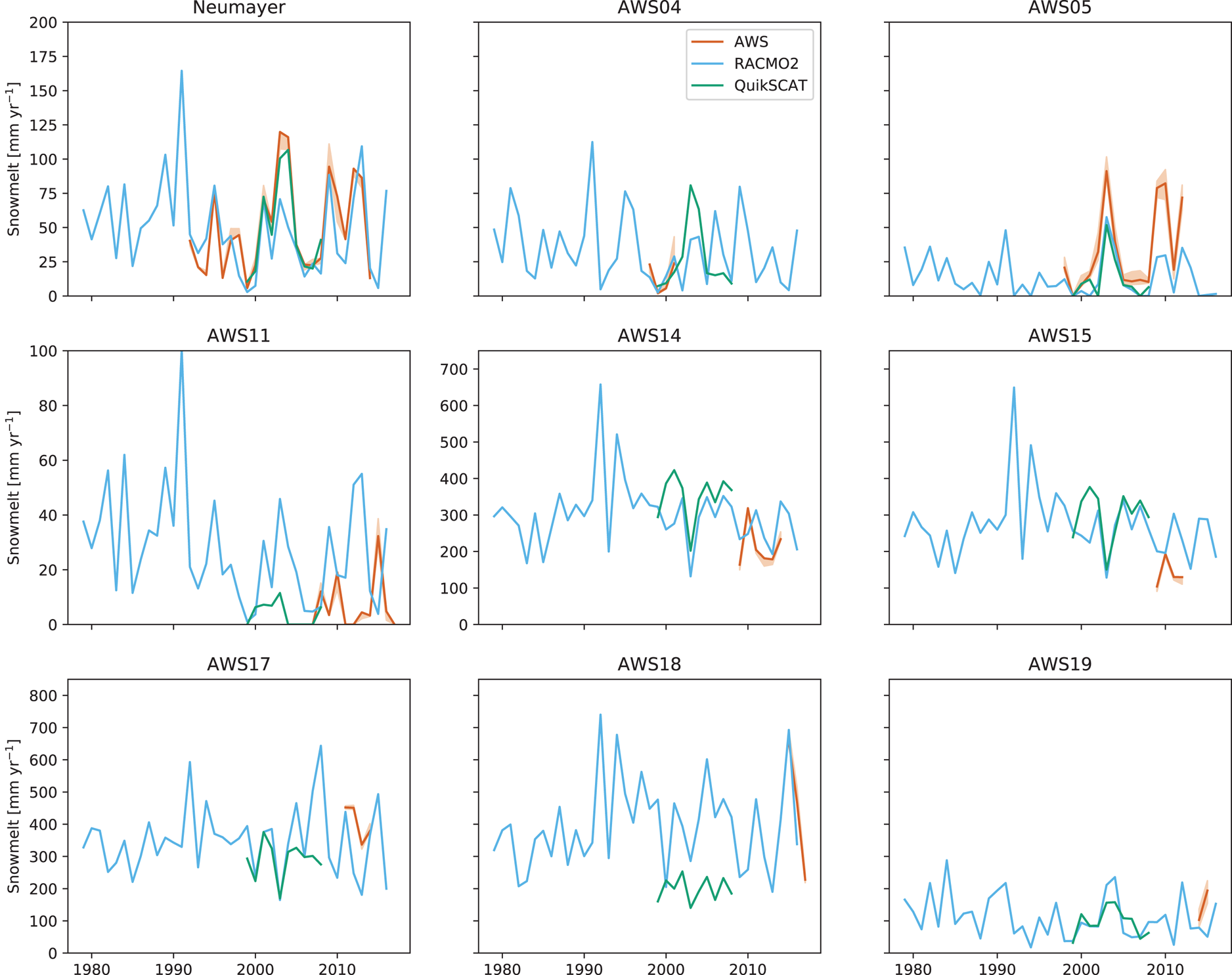
Fig. 6. Time series of in situ melt rate (dark orange), RACMO2 (blue) and QuikSCAT (green). The two in situ melt values for AWS 19 (bottom right) cover only the summer months December–February and November–January respectively, and therefore do not fully capture the melt seasons.
Figure 2 compares observed seasonal SEB cycles with RACMO2 (dashed lines). Qualitatively, the modelled seasonal cycles compare well to the observed ones. The lag in LWnet compared to SWnet is represented well by the model, as well as average and month-to-month variations in wind speed. As the fluxes are generally small, minor differences in one flux can have large implications for the total SEB. At AWS 14, modelled winter temperatures are ~ 4°C higher than observed. As a result, wintertime Q S and LW↓ are larger and LW↑ is more negative because of the higher surface temperature. At AWS 5, modelled temperatures are slightly lower than observed. Furthermore, modelled SW↑ is larger in summer, indicating a higher modelled surface albedo. As a result, Rnet is lower throughout the summer season. LW↑ is less negative, indicating a lower surface temperature, which leads to a greater surface-to-air temperature gradient and larger Q S. At Neumayer, RACMO2 models higher winter temperatures, leading to larger Q S in winter. The modelled surface albedo is higher in summer, as SW↑ is larger. As a result, modelled R net is lower in summer, leading to slightly less surface melt. The possibility to perform such detailed SEB comparisons underlines the usefulness of the in situ SEB and melt data.
QuikSCAT
As a final application we present a comparison of our melt dataset with satellite-derived melt amounts. Trusel and others (Reference Trusel, Frey, Das, Kuipers Munneke and Van den Broeke2013) present 1999–2009 annual (July–June) continent-wide maps of cumulative surface melt on a 8–10 km effective resolution. It is based on data from the SeaWinds radar scatterometer onboard the QuikSCAT satellite. The detection of liquid water in the snowpack relies on the high dielectric constant of liquid water compared to snow. As a result, radar backscatter is greatly reduced in the presence of liquid water, which is detectable even at small amounts in the snowpack. The method used by Trusel and others (Reference Trusel, Frey, Das, Kuipers Munneke and Van den Broeke2013) calibrates seasonally summed reductions in radar backscatter during melt with in situ melt products from AWS across Antarctica. AWS 14, 15 and Neumayer are among the stations that were used for the calibration, stations of which the meteorological data are also part of this study.
Figure 5c compares annual surface melt rates from QuikSCAT (1999–2009) with the in situ melt rates. Unfortunately, the overlap in time period available for QuikSCAT and our dataset is limited, resulting in data from only four stations available for the comparison. Data from Neumayer are dominating the comparison, which shows a good correlation (R 2 = 0.92). Note that since data from Neumayer were used to calibrate QuikSCAT, these results are not independent. If the Neumayer values are omitted from Figure 5c, the correlation coefficient increases (R 2 = 0.98) but the slope becomes significantly smaller than one. Figure 5c furthermore shows that all in situ surface melt rates for AWS 4, 5 and 11 are higher than those from QuikSCAT. As melt is intermittent in DML, it is possible that some melt events occur between consecutive passes of the QuikSCAT satellite. As melt amounts are low at AWS 4, 5 and 11, this affects the QuikSCAT signal more strongly at those sites than at Neumayer.
The QuikSCAT surface melt estimates are displayed in green in Figure 6, allowing for a direct comparison with the in situ and RACMO2 annual melt rates. Unfortunately, there is little temporal overlap between the QuikSCAT data and the in situ observations. Nevertheless, Figure 6 shows that the interannual variability as observed and as modelled by RACMO2 are similar, adding confidence to the long-term continent-wide melt estimates of RACMO2.
Summary and conclusions
This paper presents a benchmark dataset of consistent, in situ Antarctic SEB and surface melt rates at five locations in coastal DML and four locations in the eastern AP, at high temporal resolution (1–2 h).
Uncertainties in the in situ surface melt and energy-balance calculations are based on SEB model parameter uncertainty (Jakobs and others, Reference Jakobs, Reijmer, Kuipers Munneke, König-Langlo and Van den Broeke2019). The results show that DML and the eastern AP have very different melt climates. In the relatively cold climate of DML, melt is driven by absorption of solar radiation, with melt occurrence and rate determined by a delicate balance between processes that add (absorption of shortwave radiation) and remove (sublimation) heat from the surface. Melt is more extensive in space and time on the ice shelves in the eastern AP, owing to their more northerly location and frequent föhn events (e.g. Turton and others, Reference Turton, Kirchgaessner, Ross and King2018; Wiesenekker and others, Reference Wiesenekker, Kuipers Munneke, Van den Broeke and Smeets2018). These föhn events can lead to continuous melting for multiple days, even outside summer, but our analysis shows that continuous melt is confined to the foot of the AP mountains and does not extend far onto the ice shelf.
Despite the relatively short timeseries of the in situ melt rates and SEB, they are powerful tools to calibrate/validate/evaluate other melt products such as temperature–index models, regional climate models and satellite products. We show that temperature index models are unsuitable to estimate melt rates in the intermittent melt climate of coastal Antarctica. On the other hand, seasonal melt rates from the QuikSCAT satellite (Trusel and others, Reference Trusel, Frey, Das, Kuipers Munneke and Van den Broeke2013) and the regional climate model RACMO2 (Van Wessem and others, Reference Van Wessem2018) agree generally well with the in situ data. Although at some locations surface melt is not reproduced properly by RACMO2, for example at AWS 19 (Fig. 5), the correlation with the entire dataset is very high (R 2 = 0.83 in Fig. 5a), providing confidence in the performance of these melt products.
These pilot applications demonstrate the value of consistently derived in situ surface melt and energy-balance products from the Antarctic ice sheet, and stress the urgent need for similar observations from other coastal Antarctic sites.
Acknowledgments
The data are available on the PANGAEA data repository: doi: 10.1594/PANGAEA.910484. We would like to thank Jan Lenaerts and Stef Lhermitte for providing data of AWS 19. We furthermore thank the referees and editor Nicolas Cullen for their constructive comments. This research has been supported by the Nederlandse Organisatie voor Wetenschappelijk Onderzoek (grant no. 866.15.204). Michiel van den Broeke acknowledges support from the Netherlands Earth System Science Centre (NESSC).


 Open access