


1. Introduction
Lagrangian coherent structures (LCSs) are frame-indifferent and material flow features with exceptional qualities when compared with neighbouring structures. Fundamental to the Lagrangian study of fluid flow is the flow map
 \begin{equation} F_{t_0}^{t}(\boldsymbol{x}_0)=\boldsymbol{x}(t; t_0, \boldsymbol{x}_0) \quad \boldsymbol{x}\in\mathbb{R}^3, \quad t\in[ t_0, t_f] \end{equation}
that takes a fluid particle from its initial position  $\boldsymbol {x}_0$ at time $t_0$, to its current position $\boldsymbol {x}(t; t_0, \boldsymbol {x}_0)$ at time $t$, according to a velocity field $\boldsymbol {v}(\boldsymbol {x},t)$. The right Cauchy–Green strain tensor, $\boldsymbol{\mathsf{C}}(\boldsymbol {x}_0)=\boldsymbol {\nabla } F_{t_0}^{t}(\boldsymbol {x}_0)^\mathrm {T} \boldsymbol {\nabla } F_{t_0}^{t}(\boldsymbol {x}_0)$, plays a prominent role in objective descriptions of Lagrangian deformation and LCS extraction algorithms, the most common of which is the finite time Lyapunov exponent (FTLE) (Haller Reference Haller2015). For incompressible three-dimensional (3-D) flows, $\boldsymbol{\mathsf{C}}(\boldsymbol {x}_0)$ is symmetric, positive definite with unit determinant. That is, its eigenvalues $\lambda _i$ can be ordered such that
 \begin{equation} 0<\lambda_1\le\lambda_2\le\lambda_3, \quad \lambda_1\lambda_2\lambda_3=1, \quad 0<\lambda_1 \le 1\le \lambda_3. \end{equation}
 In  $n$-dimensional flows, the FTLE at a point $\boldsymbol {x}_0$, $\varLambda _n(\boldsymbol {x}_0)=({1}/({t_f-t_0}))\log (\lambda _n)$ represents the maximal degree of stretching of fluid initially at the point $\boldsymbol {x}_0$, from $t_0$ to $t_f$. In 2-D flows, $\lambda _2$ uniquely determines $\lambda _1$ via the unit determinant, and 2-D FTLE plots succinctly describe stretching over a given time window. However, in 3-D incompressible flows, the deformation of a sphere has two degrees of freedom, and additional information about fluid deformation quantified by $\lambda _1$ and $\lambda _2$ is not determined by FTLE alone (figure 1). There are currently no LCS diagnostics that present this higher-dimensional stretching information in a single visualization or metric.

Figure 1. One-dimensional and 2-D axisymmetric deformation of a fluid sphere, with corresponding Cauchy–Green eigenvectors,  $\boldsymbol{\xi} _i$.
The diffusion barrier strength (DBS), an LCS diagnostic that identifies diffusive transport barriers, utilizes the trace of time-averaged  $\boldsymbol{\mathsf{C}}$, and thus combines information of all three eigenvalues (Haller et al. Reference Haller, Katsanoulis, Holzner, Frohnapfel and Gatti2020). The trace, however, maps the eigenvalue space onto a 1-D subspace. In this way, both DBS and FTLE fields provide a 1-D presentation of deformation in a system that cannot be fully described by fewer than two scalars. The last notable frame-indifferent method for quantifying Lagrangian stretching is relative dispersion (Haller & Yuan Reference Haller and Yuan2000). Again, this method provides a single scalar field and only a 1-D representation of particle pair separation. There are thus currently no methods available for visualizing, or compactly representing, the geometry of 3-D stretching along hyperbolic LCS in a single plot.
In the present work, we develop a novel barycentric map to compactly describe the 3-D material deformation of fluid in physical space. Barycentric coordinates date back to the work of Möbius and define the position of a point by its distances from vertices of a simplex (Möbius Reference Möbius1827). Barycentric coordinates have since become a common tool for computer visualizations and computational mechanics (Hormann & Sukumar Reference Hormann and Sukumar2018). In turbulent flows, barycentric coordinates have also proved useful for visualizing statistical descriptions of the Reynolds stress. Specifically, the Lumley triangle has long been used as a way to describe turbulence invariants and anisotropy in fluctuating velocity components (Lumley & Newman Reference Lumley and Newman1977; Pope Reference Pope2000). A recent adaptation of the Lumley triangle has utilized a barycentric triangle representation of eigenvalue metrics to describe anisotropy and the stability of the atmosphere (Banerjee et al. Reference Banerjee, Krahl, Durst and Zenger2007; Stiperski & Calaf Reference Stiperski and Calaf2017; Stiperski, Calaf & Rotach Reference Stiperski, Calaf and Rotach2019).
We present a method for mapping the 2-D space spanned by  $\boldsymbol{\mathsf{C}}$ eigenvalues, and their associated stretching exponents, to barycentric coordinates to determine the dimension of the underlying stable and unstable manifolds in 3-D non-stationary fluid flow. These invariant manifolds control the shape of the Lagrangian deformation of fluid and their dimension in physical space provides a convenient way to describe that deformation. We define each vertex of a 2-simplex (triangle) to represent a unique end state: 1-D axisymmetric stretching, 2-D axisymmetric stretching or a 3-D isometry of fluid. The distance to the vertices represents the local deformation of the fluid being studied. In contrast to the Lumley triangle where end states represent shapes in the eigenspace of the Reynolds stress tensor, we are instead describing physical fluid deformation in an objective and material way.
We provide several motivating examples that examine advantages for identifying 3-D fluid structures with barycentric coordinates over scalar fields, and novel metrics for describing the geometry of invariant manifolds in the flow. We also compare our visualizations with FTLEs and common diagnostics for studying wall-bounded turbulent flows.
2. Methods
2.1. Linear eigenvalue ratios
A simple barycentric map representing the three idealized states of deformation can be defined directly from the eigenvalues of the Cauchy–Green strain tensor,  $\boldsymbol{\mathsf{C}}$. To do this, we first normalize the eigenvalues so that they sum to one, $\tilde {\lambda }_i={\lambda _i}/{\sum _j \lambda _j}$. In this way, every combination of eigenvalues can be represented as a convex combination of barycentric coordinate vectors, and be mapped to the interior of a 2-simplex (triangle). We map from the eigenvalue space to a barycentric coordinates system, $(C_1, C_2, C_3)$ via
 $$\begin{gather} C_1 = \tilde{\lambda}_3-\tilde{\lambda}_2, \end{gather}$$
 $$\begin{gather}C_2 = 2(\tilde{\lambda}_2-\tilde{\lambda}_1), \end{gather}$$
 $$\begin{gather}C_3 = 3\tilde{\lambda}_1. \end{gather}$$
For each coordinate,  $C_i=1$ corresponds to the limiting states of deformation defined in table 1. This linear mapping provides a simple tool for compactly representing the role of all three $\boldsymbol{\mathsf{C}}$ eigenvalues in fluid deformation, and estimating the dimension of invariant manifolds. The study of LCSs typically focuses on the rate of stretching of fluid, however, which requires a more complex map to represent in barycentric coordinates. We develop that map in the following section, and it remains the focus of the examples in the rest of this study. The techniques of stretching coordinate analysis, however, equally apply to our initial linear barycentric eigenvalue coordinate system.
Table 1. Relationship of Cauchy–Green strain tensor eigenvalues, barycentric coordinates, invariant manifolds and resulting deformation of a sphere.

2.2. Stretching exponent representation
To more directly represent the rate of stretching in a time-varying velocity field, we approximate the stretching exponents as defined as the natural logarithm of the  $\boldsymbol{\mathsf{C}}$ eigenvalues. Mapping the stretching exponents to barycentric coordinates is a considerably more complex task as $\ln (\lambda _1)$ is negative and unbounded below, $\ln (\lambda _3)$ is unbounded above and $\ln (\lambda _2)$ is unbounded both above and below. We perform a series of transformations to make the stretching exponents more easily manipulated and represent each state of fluid stretching with strictly non-negative barycentric coordinates (inside a triangle). By initially adding one to each eigenvalue, we guarantee non-negative exponents for $\lambda _1$ and $\lambda _2$. The transformed exponents, $\hat {\varLambda }_i=\ln (\lambda _i+1)$, satisfy
 \begin{equation} 0<\hat{\varLambda}_1<\hat{\varLambda}_2<\hat{\varLambda}_3<\infty, \quad \hat{\varLambda}_1\le\ln(2)\le\hat{\varLambda}_3. \end{equation}
From here, the stretching exponent coordinate system is defined as
 \begin{gather} \hat{C}_1 = \hat{\varLambda}_3-\hat{\varLambda}_2, \end{gather}
 \begin{gather} \hat{C}_2 = \hat{\varLambda}_2-\hat{\varLambda}_1, \end{gather}
 \begin{gather} \hat{C}_3 = \frac{1}{\ln(2)-\hat{\varLambda}_1}-\frac{1}{\ln(2)}. \end{gather}
Lastly, we normalize the  $\hat {C}_i$ vectors such that $\sum C_i = 1$, as before. Each limiting state, $C_i=1$, is equivalent to those defined by the simpler linear eigenvalue ratios in table 1. By representing these modified the stretching exponent, $\hat {\varLambda }_i$, barycentrically, we can more closely relate our findings to the Lyapunov exponents standard in the dynamics literature. As shown in the following examples, visualizing the barycentric stretching exponent map as red-blue-green (RGB) vectors provides the same level of detail as FTLE plots, while also providing additional information about deformation and invariant manifold geometry.
As was originally derived for anisotropy tensors by Banerjee et al. (Reference Banerjee, Krahl, Durst and Zenger2007), both the linear and exponential coordinate systems can be mapped into a Cartesian triangle with the mapping
 $$\begin{gather} x_b=C_1+\frac{C_3}{2}, \end{gather}$$
 $$\begin{gather}y_b=C_3\frac{\sqrt{3}}{2}. \end{gather}$$
This triangle is shown in figure 2 and compactly represents all possible states of deformation for an initial sphere in a frame-indifferent and material manner. That is, for an initial sphere of fluid under advection in an incompressible flow, the final shape of that sphere is uniquely represented by coordinates  $(C_1, C_2, C_3)$, with larger values in any dimension representing a stronger influence of the respective invariant manifolds. The $C_i$ coordinates easily map to any linearly independent set of RGB vectors and can be used to visualize the shape of deformation and the role of all three $\boldsymbol{\mathsf{C}}$ eigenvalues in a single image. In this work, we use a canonical map to red, green and blue vectors as is common in the Reynolds stress literature (see e.g. Banerjee et al. Reference Banerjee, Krahl, Durst and Zenger2007; Stiperski & Calaf Reference Stiperski and Calaf2017; Stiperski et al. Reference Stiperski, Calaf and Rotach2019), shown in figure 2. The map defined by equations (2.5–2.7) is not unique. Varying this mapping in a way that maintains the physical meaning of the limiting states $C_i=1$, could provide a different definition of distance to each limiting state inside the simplex, while still respecting the definitions in table 1. These barycentric stretching coordinates also provide a vector quantity that can be used for analysis of flow geometry in different regions or different flows.

Figure 2. Barycentric Cauchy–Green eigenvalue triangle relates the colouring scheme for fluid deformation visualization, the limiting states coordinates and the dimension of unstable invariant manifolds to the eigenvalue relationships.
Of additional interest to the fluid dynamics community is the role of rotationally coherent structures, vortices. A natural extension of the present work is an inclusion of rotational information with fluid stretching. In the Appendix, we show how a similar bilinear approach can quantify and visualize combined rates of material rotation and deformation. The combined stretching and rotation methods do not utilize limiting states of fluid particle motion and are less technically involved. Even so, we show that more informative qualitative and quantitative analysis can be performed when combining rates of stretching and rotation for 2- and 3-D examples.
3. Results
3.1. Stable and unstable manifolds
The main strength of the new barycentric mapping of Lagrangian stretching exponents is their ability to identify not only the degree of stretching, but also the dimension of stable and unstable manifolds in a flow. We verify this claim by analysing finite time advection of fluid particles surrounding the Burgers–Rott vortex (Burgers Reference Burgers1948; Rott Reference Rott1958). We can write this stationary solution to the Navier–Stokes equations in Cartesian coordinates as
 $$\begin{gather} u_x={-}\xi x-\frac{\varGamma}{2 {\rm \pi}r^2}(1-{\rm e}^{-({r^2 \xi}/{2\nu})})y, \end{gather}$$
 $$\begin{gather}u_y={-}\xi y+\frac{\varGamma}{2 {\rm \pi}r^2}(1-{\rm e}^{-({r^2\xi}/{2\nu})}), x \end{gather}$$
 $$\begin{gather}u_z=2\xi z, \end{gather}$$
where  $r=\sqrt {x^2+y^2}$, and choose the parameters $\xi =0.042$, $\varGamma =1.45$ and $\nu =0.01$.
This model of vortical flow consists of a 2-D stable (repelling) manifold on the  $z=0$ plane and a line vortex on the $z$-axis acting as an unstable (attracting) manifold, in forward-time advection. In backward-time advection, the $x$–
$x$– $y$ plane is unstable, and the $z$-axis is stable. Streamlines initiated on the $z=\pm 0.1$ planes surrounding the forward time Burgers–Rott vortex, and the underlying forward-time stable (green) and unstable (red) manifolds can be found in figure 3(a).

Figure 3. Burgers–Rott vortex streamlines and underlying invariant manifolds (a), forward BSM (b), backward BSM on the  $z=0.1$ plane (c).
In figure 3(b), the RGB barycentric stretching map (BSM) of a subsection of the  $z=0.1$ plane shows the dominant influence of the core line vortex (1-D unstable manifold) over an integration time $t_f-t_0=70$. Large $C_1$ corresponds to the predominately axisymmetric one-component stretching and dominance of the largest eigenvalue (FTLE) over the other two eigenvalues. Under backward-time advection over the same window (figure 3c), we see that significant two-component axisymmetric stretching is occurring for the majority of the domain, but in the immediate neighbourhood of the line vortex, there is still significant 1-D deformation. This is an effect of finite time advection when fluid particles are in transition from stable to unstable manifolds, or finite time approximations to asymptotic behaviour. That is, the strong rate of rotation and fluid stretching around the central vortex outweighs the stretching along the $x$–
$x$– $y$ plane for fluid adjacent to the vortex over short time periods. As $t_f-t_0$ goes to infinity, the unstable manifold effectively attracts all fluid parcels from the $z=0.1$ plane, and flattens them in a two-component axisymmetric fashion. At longer finite integration times (e.g. $t_f-t_0=10^4$), this effect is already evident and replaces figure 3(c) with a purely green field. This sensitivity to integration time highlights the degree to which the local geometry of deformation is determined by the BSM field.
3.2. Stationary concentrated vortex model
The stationary concentrated vortex model (SCVM) is a steady axially symmetric solution to the Euler equations that represents vortices in the Earth's atmosphere with finite spatial extent, such as dust devils and tornados (Onishchenko et al. Reference Onishchenko, Fedun, Horton, Pokhotelov, Astafieva, Skirvin and Verth2021). The vortex is concentrated in both the radial and vertical directions and consists of two distinct inner and outer regions, an internal upward motion and external downward motion. The vortex is also divided vertically into a centripetal flow in the bottom and centrifugal flow at the top with upward moving fluid recirculated from the top of the vortex back down. The velocity components can be written in cylindrical coordinates as
 $$\begin{gather} v_r ={-}v_0 \frac{r}{L} \left( 1-\frac{z}{L} \right)\exp\left({-\frac{z}{L}-\frac{r^2}{r_0^2}}\right), \end{gather}$$
 $$\begin{gather}v_\theta ={\pm} v_{\theta_0}\frac{z}{L}\exp\left({-\frac{z}{L}-\frac{r^2}{r_0^2}}\right), \end{gather}$$
 $$\begin{gather}v_z = 2v_0 \frac{z}{L} \left( 1-\frac{r^2}{r_0^2}\right)\exp\left({-\frac{z}{L}-\frac{r^2}{r_0^2}}\right), \end{gather}$$
where  $r_0$ is the radial extent separating inner and outer vortex structures, $L$ is the height of maximum vertical velocity at $r=0$ and $v_0$ and $v_{\theta _0}$ are characteristic velocities. For our example, we use $v_0 = 1$, $L = 10$, $r_0 = 10$ and $v_{\theta _0}=9$.
We analyse the nested SCVM structures in BSM fields and compare with FTLE values in figure 4. Both FTLE and BSM plots highlight the outermost boundary of the vortex, as well as the edges of the internal spiral structure. The strongest 1-D deformation, shown in red in figure 4(a), is verified through direct advection in figure 4(c). Fluid in this region coincides with the FTLE ridge in figure 4(d). An initially small sphere located where the maximal  $C_1$ value is found (black dot in figure 4a) is advected in the flow for $t_f-t_0=500$. The resulting shape (red band) was translated back to the origin to compare with other limiting state shapes. This long red band is the result of 1-D axisymmetric deformation along a 1-D unstable manifold, as predicted.

Figure 4. Examining the stationary concentrated vortex structure through the Cauchy–Green eigenvalue BSM (a), stretching coordinates (b), shapes of advected fluid spheres (c) and FTLEs (d).
The innermost core, where ascending fluid rises to the top of the vortex before spreading laterally and descending, is separated from the outer regions in the BSM field as a distinct  $C_2$ (green) structure. This region is a great example of the strength of BSM for visualizing both degrees of freedom in 3-D incompressible fluid stretching. Relatively low $\lambda _3$ values lead the FTLE map to prescribe similar values in the $C_2$ vortex core as outside the vortex domain. However, in this zone, small $\lambda _1$, relatively large $\lambda _2$ and moderate $\lambda _3$ values result in a distinct flattening of fluid parcels, as shown by the advected $C_2$ limiting case sphere in figure 4(c) (green disk). This behaviour is distinct from both the outer region of the vortex, as well as the region outside the vortex, and is not visible from the FTLE field alone.
The region outside the concentrated vortex is shown with high  $C_3$ values, and low FTLE values, as $\lambda _1$ is close to 1. Here, fluid parcels are not deformed, as is shown by the small blue sphere of advected fluid in figure 4(c) originating at the black dot in panel (a). We can further define the 3-D structure of the SCVM by extracting $C_i$ isosurfaces. In figure 5, we show isosurfaces of $C_i=0.75$ for $i\in \{1, 2, 3\}$ overlaid on SCVM streamlines coloured in grey scale by their trajectory stretching exponents (Haller, Aksamit & Bartos Reference Haller, Aksamit and Bartos2021). While trajectory stretching exponents do not separate the flow domain to the same degree of detail as BSM, shading of the rising inner core (white) and lower outer recirculating core (black) complements the structural information provided by streamlines alone.

Figure 5. Isosurfaces separating end-state regions of the stationary concentrated vortex with vortex streamlines coloured by the trajectory stretching exponent.
The innermost  $C_2$ core consists of fluid that quickly rises to the top of the vortex, before descending on the outer regions of the flow, whereas immediately adjacent fluid with positive vertical velocity is recirculated in the lower vortex spirals, contained in the strong $C_1$ regions. This separation is not evident from the velocity profiles alone. The distinction of the $C_1$ and $C_2$ regions is supported by the FTLE fields, but as mentioned before, the responsible invariant manifold, or shape of fluid deformation, is indistinguishable from regions outside the vortex domain. The outermost $C_3$ isosurface separates the fluid with minimal motion, as can be seen by streamlines in the outer domain with minimal length.
The balance of these distinct vortex features is shown in figure 4(b). Each  $(x_b, y_b)$ coordinate represents one initial condition of fluid from figure 4(a). This presentation provides additional quantifiable insight into the flow structure. For example, there are no regions with $\lambda _1=\lambda _2$, except when $\lambda _3$ is exceptionally large or small. The black marker indicates the centre of mass for this distribution of barycentric coordinates, $(C_1, C_2, C_3) = (0.65, 0.18, 0.17)$, and represents the relative presence of 1-D and 2-D stretching, and isometric regions in the flow domain. This simple mean also provides a basis for distinguishing similar flows, as we shall show in the next section.
Upon slightly modifying the SCVM model, we present another example of the enhanced utility of harnessing all  $\boldsymbol{\mathsf{C}}$ eigenvalues for understanding 3-D flows. We reduce the rate of rotation by setting $v_{\theta _0}=1$, and increase the characteristic vertical velocity to $v_0 = 5$. This generates a much simpler plume structure over finite times in the core of the SCVM. Advecting particles initially on the $z=5$ plane for a transport time $t_f-t_0=20$, we can calculate the BSM and FTLE fields, and map their values on the final position of the fluid surface. This deformed surface can be seen in figure 6.

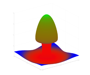
Figure 6. The BSM (a) and FTLE (b) fields plotted on the final position of fluid particles advected from the  $z=5$ plane in the SCVM. The stem in the centre of the vortex appears as both strong FTLE and single-component BSM values. The BSM reveals the 2-D deformation of the fluid in the cap, whereas FTLE values reveal a degree of stretching similar to the outer regions of the vortex and are unable to distinguish this feature.
Fluid in the annulus  $15< r<21$ is stretched towards and up the central core of the vortex. This results in a distinct stem formation with both large FTLE and single-component BSM values. Fluid particles with $r<15$ are quickly transported vertically, and then spread in a distinctly two-component fashion along the cap structure seen in figure 6. These fluid particles are attracted to an unstable manifold distinct from the vortex core in the flow. With the BSM map, we are able to distinguish the cap, stem and surrounding fluid field. In contrast, focusing solely on the largest eigenvalue with FTLE, we are able to distinguish the cap from the stem, but do not know the cap fluid is actually deforming in a different manner than that at radial distance $r=19$.
3.3. Case of Arnold–Beltrami–Childress flow
As a third example, we consider the 3-D steady Arnold–Beltrami–Childress (ABC) flow (Dombre et al. Reference Dombre, Frisch, Greene, Henon, Mehr and Soward1986) on the triply periodic domain  $U=[0, 2{\rm \pi} ]^3$,
 \begin{equation} \boldsymbol{v}(\boldsymbol{x},t)=\begin{pmatrix}A\sin x_{3}+C\cos x_{2}\\ B\sin x_{1}+A\cos x_{3}\\ C\sin x_{2}+B\cos x_{1} \end{pmatrix}. \end{equation}
 Following the parameter space study by Dombre et al. (Reference Dombre, Frisch, Greene, Henon, Mehr and Soward1986), we consider two distinct cases of the flow in figure 7. In panels (a,b,c), we show FTLE, BSM and the stretching triangle for  $A=1$, $B=\sqrt {2/3}$ and $C=\sqrt {1/3}$, over an integration time $t_f-t_0=100$. This is a commonly studied example where the six principal vortices are present. As a second case, we advect fluid particles for the same integration time with the parameters $A=1$, $B=0.145789$ and $C=0.145789$, when a double resonance is present (Dombre et al. Reference Dombre, Frisch, Greene, Henon, Mehr and Soward1986). The difference between the two choices of parameters is qualitatively evident when comparing the FTLE or BSM fields from panels (a,b,c) and (d,e,f) of figure 7, as several of the six principal vortices have clearly collapsed.

Figure 7. Finite time Lyapunov exponents, BSM and stretching coordinates for the ABC flow: (a–c)  $A=1$, $B=\sqrt {2/3}$ and $C=\sqrt {1/3}$; (d–f) $A=1$, $B=0.145789$ and $C=0.145789$.
For the six-vortex ABC flow (panels a–c), the highly chaotic regions are identified by large FTLE values surrounding the Kolmogorov–Arnold–Moser (KAM) surfaces. In the BSM field, this region is dominated by strong 2-D stretching. This is distinct from the dimension of deformation occurring in the SCVM example where the most significant fluid stretching (largest FLTE) was primarily along 1-D unstable manifolds. The strong shear layers separating the KAM surfaces (six vortices) are correctly identified with large  $C_2$ (two-component axisymmetric), and are extracted as $C_2=0.5$ isosurfaces in figure 8.

Figure 8. The  $C_2$ and $C_3$ isosurfaces in the six-vortex ABC flow identify vortex cores and separating shear layers.
The stretching coordinates (figure 7c, f) provide another view of this flow dynamics. For the six-vortex ABC flow, the Cauchy–Green strain tensor is dominated by small  $\lambda _1$ values ( $y_b\approx 0)$, significant chaotic $C_2$ regions and a dominance of 1-D deformation tangent to the KAM surfaces. There are few points in isometric (pure translation/rotation) regions, as shown in the stretching coordinate triangle, the BSM and $C_3=0.3$ isosurfaces in figure 8. The centre of mass for the barycentric stretching coordinates reveals the relative balance of these structures with a value of $(0.687, 0.312, 5\times 10^{-4})$, marked in black in figure 7(c).
In contrast, for the double resonance case (d–f), we find much weaker shear layers, and smaller chaotic regions surrounding the four principal  $x$–
$x$– $y$ vortices noted by Dombre et al. (Reference Dombre, Frisch, Greene, Henon, Mehr and Soward1986), as well as much larger isometric regions. This is reflected quantitatively in a barycentric stretching centre of mass with a smaller $C_2$ influence and larger $C_3$, $(0.83, 0.16, 0.01)$, marked in black (figure 7f). Additionally the stretching coordinates now show a much broader range of features present in the flow as more of the triangle is filled in, providing a qualitative fingerprint of the shape of material flow structures.
3.4. Turbulent channel flow
Lastly, we examine data from the publicly available Johns Hopkins University Turbulence Database (JHTDB) direct numerical simulation of a  $Re_{\tau }=1000$ channel flow (Perlman et al. Reference Perlman, Burns, Li and Meneveau2007; Li et al. Reference Li, Perlman, Wan, Yang, Burns, Meneveau, Burns, Chen, Szalay and Eyink2008; Graham et al. Reference Graham2016). The JHTDB channel flow is available on a $2048 \times 512 \times 1536$ grid for a domain of size $8{\rm \pi} h \times 2h \times 3{\rm \pi} h$, where $h$ is the half-channel height. All figure coordinates will be displayed in dimensionless half-channel height units ( $h=1$). This dataset has been used in a large number of turbulence studies, including recently by Aksamit & Haller (Reference Aksamit and Haller2022) to study the structure and organization of objective momentum transport barriers.
In figure 9(a) we present BSM for fluid particles in a streamwise–wall-normal  $1.5h \times 2h$ section of the $z=3$ plane. This is the same region used for momentum barrier tracking by Aksamit & Haller (Reference Aksamit and Haller2022). We calculated the Cauchy–Green strain tensor for a $2000\times 2000$ grid of initial conditions, over $t_f - t_0 = 200\delta t$ (channel flow-through times). Figure 9(b) shows the mean streamwise velocity profile in the plane, and figure 9(c) shows the instantaneous streamwise velocity field at time $t_0$, a diagnostic common to boundary layer structure discussions (Adrian, Meinhart & Tomkins Reference Adrian, Meinhart and Tomkins2000; Kwon et al. Reference Kwon, Philip, De Silva, Hutchins and Monty2014; De Silva, Hutchins & Marusic Reference De Silva, Hutchins and Marusic2015).

Figure 9. Comparison of the BSM of Cauchy–Green eigenvalues (a), the average streamwise velocity profile (b), instantaneous streamwise velocities (c), stretching coordinate distribution (d) and streamwise velocity distribution (e). Streamwise velocity contours in (c) correspond to marked local minima in (e). The arrow in (a,c) identifies low velocity fluid as it enters the quiescent core.
We averaged the stretching coordinates  $C_i$ in wall-parallel planes to obtain an average stretching coordinate profile in figure 9(d). As in FTLE studies of turbulent boundary layers (e.g. Green, Rowley & Haller Reference Green, Rowley and Haller2007; Haller et al. Reference Haller, Katsanoulis, Holzner, Frohnapfel and Gatti2020), there is a clear influence of the shear generated by both channel walls on the material deformation of the flow. The highly turbulent near-wall region is characterized by strong 1-D deformation, as evidenced by the dominance of red regions in BSM plot and the mean stretching coordinates near the $C_1=1$ corner for the $y=-1$ plane (figure 9d). As we begin to traverse the channel, $\lambda _1$ and $y_b$ remain small, indicating a high degree of fluid deformation. Planar interfaces begin to appear as green curves in the BSM field as $y$ increases, and $x_b$ migrates towards zero while $y_b$ stays close to zero. This suggests the presence of organizing internal interfaces, or 2-D unstable manifolds, along which the fluid is spreading and separating high mixing ( $C_1$) regions.
At approximately  $y=-0.8$, pockets of limited fluid deformation (blue regions) begin to appear, and $y_b$ values begin to increase. This suggests the presence of small pockets of relatively undisturbed fluid behind turbulent coherent structures. This is representative of sheltering of fluid that occurs behind ramps or large scale motions that peel off of the wall into the faster moving channel core. In figure 9(c), we see this is approximately the location where the streamwise velocity deviation is close to zero, and the maximal extent of the low velocity bulge outlined by $v_x=1.04$.
As we traverse further into the relatively quiescent core of the channel, one can see patches of energetic stretching, surrounded by primarily blue, nearly isometric regions. This confirms that, on these time scales, stretching inside the channel core is much less influential than pure translation or rotation. This is also evident in the mean stretching coordinates where the  $y=0$ average is close to the $C_3=1$ limiting state. Symmetric behaviour can be seen as one approaches the $y=1$ wall, as well as a large scale ramp of turbulent fluid peeling off the $y=1$ wall into the channel core.
This examination is complemented by the standard tool for uniform momentum zone analysis, the streamwise velocity histogram (figure 9e). Several distinct uniform momentum zones can be identified as velocity peaks in the histogram. The separating interfaces are drawn as  $v_x$ contours corresponding to minima between these peaks in figure 9(c). While there is some loose qualitative agreement between momentum zones and LCSs, it is important to remember that momentum zone designations are Eulerian in nature, not frame-indifferent and thus not designed to extract material fluid structures. Rather, they are used to discuss streamwise momentum organization. Even so, there are some insightful conclusions that can be drawn from the BSM plots. For example, the isometric blob at approximately $(6, -0.85)$ originates in a protected region behind a slow, $v_x=0.76$, ramp leaving the wall. As well, the edge of the quiescent core (Kwon et al. Reference Kwon, Philip, De Silva, Hutchins and Monty2014) at $v_x=1.04$ correlates with the edge of dominant isometric motion, especially in the upper half of the channel.
We have also used arrows to highlight a relatively low velocity region of fluid above the  $v_x=0.76$ contour in figure 9(a,c). This fluid has positive wall-normal velocity (figure 10a), and deforms as it encounters the faster moving, but less turbulent, core of the channel. The top of this slowly moving fluid is highlighted by a ridge of quasi-planar two-component stretching (figure 9a), similar to that seen along the cap of figure 6. We can resolve even finer structure details in this highly turbulent near-wall region by following the momentum barrier field analysis of Aksamit & Haller (Reference Aksamit and Haller2022).

Figure 10. Comparison of vertical velocity fields (a) with the BSM (b) calculated in the momentum barrier field at time  $t_0$. Specific contours of streamwise and wall-normal velocities are overlaid in both panels. The aBSM plot reveals objective momentum barrier structures and provides a much greater degree of structural detail than frame-dependent velocity fields.
To identify momentum transport barriers, we first advect trajectories in the instantaneous momentum barrier field at time  $t_0$, instead of the original velocity field. It has been shown that instantaneous barriers to objective momentum transport correspond to invariant manifolds in the vector field $\boldsymbol {x}'=\Delta \boldsymbol {v}$ (Haller et al. Reference Haller, Katsanoulis, Holzner, Frohnapfel and Gatti2020). By calculating Cauchy–Green eigenvalues from flow maps defined in this vector field, we can examine instantaneous barriers to momentum transport in the flow at a given time, instead of passive barriers of fluid transport. The FTLE analogue in the active barrier domain is referred to as aFTLE Haller et al. (Reference Haller, Katsanoulis, Holzner, Frohnapfel and Gatti2020). The reader is referred to Haller et al. (Reference Haller, Katsanoulis, Holzner, Frohnapfel and Gatti2020) and Aksamit & Haller (Reference Aksamit and Haller2022) for further details of this method and development of the theory.
We show BSM in the active barrier field (aBSM) in figure 10(b). In both panels of figure 10, we overlay contours of streamwise and vertical velocity. It is immediately clear that the aBSM field reveals more internal structure in the fluid flow than contours of  $v_x$ or $v_y$. Closer investigation also reveals some layering in the high shear regions near the wall. Specifically, we find much smaller momentum blocking structures below the $v_x=0.76$ contour, as could be expected in the near-wall region. Although velocity contours have no significance as a momentum blocking structure, the low streamwise values are likely a result of the turbulent structures revealed in the momentum barrier field (Aksamit & Haller Reference Aksamit and Haller2022).
Above approximately  $y=-0.8$, we transition to less densely packed structures with lower curvature. There is more space between strong momentum barriers, which corresponds to the intermittent isomorphism zones detailed in figure 9(a). Spacious regions of strong one-component mixing (red) are often delimited by two-component (green) ridges. This suggests intense internal mixing, separated by small quasi-planar interfaces. As we move further from the wall, multiple vortical momentum barriers can be found below the $v_y=0$ contour. The extent of the strongly deforming zone is seen as more isomorphic (blue) regions become present around $y=-0.6$ in both the fluid transport, and momentum transport fields (figures 9a and 10b, respectively). The uppermost reaches of the highly turbulent zone (surrounding arrow in figures 9 and 10) contains three vortical momentum barriers at the interface between the shear-driven turbulence at the wall and the quiescent core of the channel. Contours around vortex heads can be seen as circular layering of one- and two-component stretching in the aBSM field, before transitioning to the upper isomorphism region. These vortex heads are travelling away from the wall (figure 10a), and are capped above by two-component ridges described in more detail below.
The BSM and aBSM plots reveal the 3-D nature of structures in a 2-D presentation. As with all Lagrangian diagnostics, the values calculated are fundamentally linked to the user-defined integration time. For longer integration times, fluid particle behaviour becomes uncorrelated with fluid structures adjacent to initial positions where diagnostics are mapped. The flow map becomes the identity for integration times of zero. Choosing an appropriate time that balances these effects can be done with trial-and-error, or through statistics on autocorrelation functions (e.g. Aksamit & Haller Reference Aksamit and Haller2022).
In figure 11, we show the effect of longer integration times on BSM for a region surrounding the turbulence interface. At short transport times ( $t_f-t_0=80\delta t$), we see that much of the fluid has not yet had a chance to significantly deform, but the top edge of the highly turbulent zone at $y=-0.6$ is already appearing as a 2-D barrier. A transect of barycentric stretching in figure 11(e–h) quantifies the state of deformation. In figure 11(e), stretching coordinates have a centre of mass marked in black at approximately $(x_b,y_b)=(0.5, 0.7)$ confirming a generally low level of deformation. As integration time increases (figure 11b,c), more fluid stretching is revealed below the edge of the channel core, with limited changes above. The centre of mass in the barycentric stretching triangle migrates to a higher degree of deformation as more one- and two-component stretching is measured. From $t_f-t_0=160\delta t$ to $t_f-t_0=200\delta t$, the centre of mass in the stretching triangle has not significantly moved and there is qualitatively minimal structural change between figure 11(c,d). This suggests steady BSM has reached a steady state for the time being. Longer integration times would likely reveal more structure in the channel core as lower vorticity there slows the rate at which rotational fluid structures can be identified.

Figure 11. Multiple BSM plots (a–d) and barycentric stretching triangles (e–h) for increasing integration times. The edge of the highly turbulent zone appears as a two-component ridge for all integration times, but the degree of structural detail above and below the interface increases with integration time. There is also smaller change between the two longest integration times than any other pair.
We conduct a similar sensitivity analysis for aBSM surrounding vortex heads at the edge of the channel core in figure 12. As integration time increases, the edges of the two vortices becomes more well defined, and more structure above and below the vortex heads is revealed. Similar to previous comparisons, the use of all Cauchy–Green eigenvalues shows detailed two-component stretching features in aBSM plots where low aFTLE values reside. Additionally, isomorphic aBSM zones correspond to remaining low aFTLE values. At the longest integration time ( $2.5\times 10^{-4}$, figure 12c, f), aFTLE and aBSM ridges around the vortex heads become noisy. This is due to the long integration time effects mentioned earlier. At this point, even longer integrations would be detrimental as they would reduce the information presented and increase the computational burden.

Figure 12. Multiple aBSM (a–c) and aFTLE (d–f) plots for increasing integration times. There is progressively enhanced structural detail as integration time increases, but aBSM and aFTLE ridges become much noisier at the longest integration time, suggesting a saturation in structure information available. Two-component ridges (caps) appear above both vortex heads in regions of low aFTLE at all integration times.
4. Conclusions
We introduce a novel frame-indifferent and material method to quantify the dimension of invariant manifolds and represent the 3-D geometry of LCSs and momentum transport barriers in incompressible stationary and time-varying fluid flows. By mapping Cauchy–Green strain tensor eigenvalues to barycentric coordinate systems, we can visualize the shape of fluid deformation in turbulent and non-turbulent fluids. We complement the extensive literature on LCSs and strain tensor invariants with an advance in visualizing and quantifying higher-dimensional structure geometry. As analysis of barriers and transport in complex 3-D flows continues to accelerate, a method to quantify and represent the geometry of 3-D coherent structures on a static printed page holds great value for scientific communication and investigation.
Our visualization utilizes three limiting states of deformation as the basis for barycentric coordinate vectors: 1-D axisymmetric, 2-D axisymmetric deformation and 3-D fluid parcel isometries. The deformation cases also correspond to the dimension of the underlying invariant manifolds in both autonomous and non-autonomous systems. Mapping to barycentric coordinates allows a single compact visualization of flow geometry that has previously only been possible by using, at least, two separate scalar fields. We can also use the barycentric stretching coordinates to describe qualitative aspects of the flow and distinguish between similar flows. This can be especially helpful for comparing case studies or identifying specific physical phenomena.
The choice of map from eigenvalues and stretching exponents to barycentric coordinates is not unique. By fixing the limiting states, the boundaries of the stretching simplex, future research may find benefit from other maps of stretching coordinates in the interior of the stretching simplex. This would vary how quickly descriptions of the flow would transition between limiting states for intermediate conditions.
An analogue of this higher-dimensional fluid description is the combination of rates of both material stretching and rotation in one quantitative measure. We show how this can be simply performed with bilinear maps of FTLEs and Lagrangian-averaged vorticity deviation in the Appendix. This method provides further insight into how rates of stretching and rotation relate for various 2- and 3-D flows.
The methods developed here are a natural extension of the objective invariant manifold and LCS for 3-D flows. The majority of LCS studies have been performed in 2-D flows where a single Cauchy–Green eigenvalue describes deformation in the flow. This is insufficient for 3-D flows. We provide additional insights into LCS geometry and invariant manifold dimension for 3-D flows that can help inform researchers that study fluid structures without an a priori understanding of how a fluid is deforming or separating. For example, in studies of leading edge vortices, the geometry of fluid mixing can significantly augment lift forces (Eldredge & Jones Reference Eldredge and Jones2019). For convective fluid studies, we have shown that distinct parts of buoyancy driven plumes can be delimited based on how they deform in the surrounding fluid. In turbulent boundary layer flows, the dominance of top-down or bottom-up structures is not universally understood, nor is the mechanism of amplitude modulation. In these cases, more complete descriptions of fluid deformation may help objectively verify how vortices are formed and interact with the surrounding flow. Furthermore, researchers that are interested in constructing complex fluid structures from simplified building blocks would benefit from a more complete description of structure geometry and visualizations.
Funding
The author acknowledges financial support from the Swiss National Science Foundation (SNSF) Postdoc Mobility Fellowship Project P400P2 199190.
Declaration of interests
The author reports no conflict of interest.
Data availability statement
The Johns Hopkins Turbulence Database used in this study is accessible at https://doi.org/10.7281/T10K26QW. The AVISO geostrophic current velocities are openly available from the Copernicus Marine Environment Monitoring Service at http://marine.copernicus.eu.
Appendix
The techniques developed thus far provide a natural extension of hyperbolic Lagrangian coherent structure diagnostics for 3-D flows by combining multiple qualitative measures of fluid deformation. In addition to hyperbolic manifolds, there is also great interest in understanding elliptic manifolds, such as coherent rotational vortices. While fixed points ( $\lambda _3=1$) provide some indicator of elliptic regions, there are also objective tools we can utilize to address material rotation more directly. In the following, we show how fluid stretching and rotation information can be easily combined in a compact visualization for 2-D and 3-D flows.
The Lagrangian-averaged vorticity deviation (LAVD) is a widely used objective measure of material rotation for 2- and 3-D time-varying flows (Haller et al. Reference Haller, Hadjighasem, Farazmand and Huhn2016). This diagnostic provides an analogous rotational complement to Cauchy–Green eigenvalues. While stretching and rotation are intrinsically linked through the governing equations of fluid flow, rates of stretching and rotation are independent of each other. That is, high stretching and rotation regions may overlap, or be entirely uncorrelated. This is in contrast to the eigenvalues of the Cauchy–Green tensor which must follow strict relationships (1.2). Both FTLE and LAVD naturally take values between zero and infinity for incompressible flows, further simplifying visualization. For this parameter space, we propose a simple bilinear colour map, with each linear colour map normalized by either the maximum rate of stretching (FTLE) or rotation (LAVD). An example of one such colour map is shown in figure 13.

Figure 13. Example of a bilinear colour map that represents all possible values of the two independent components of material deformation, stretching (FTLE) and rotation (LAVD).
For clarity, we make two linear colour maps with visually distinct RGB values to represent maximal stretching and rotation. Both linear colour maps use the same neutral colour for zero. An example of these two colour maps can be found in panels (a,b) for three different flows in figures 14–16. Once values of FTLE and LAVD have been mapped to RGB vectors, we combine them through multiplication and this results in the stretching and rotation maps in panel (d) for figures 14–16. This combines the stretching and rotation measures and allows a compact representation of the role of each structure in the flow. Similar to the barycentric stretching triangle, each bilinear map gives a signature of the strength of hyperbolic and elliptic LCS in the flow, shown in panel (c) for the three examples.

Figure 14. Panels (a,b) show linear colour maps of FTLE and LAVD, respectively for the SCVM in figure 4. Panel (c) shows the relationship between stretching and rotation for different locations in the flow. Panel (d) reveals the stretching and rotation structures, especially the strong recirculation zone.

Figure 15. Panels (a,b) show linear colour maps of FTLE and LAVD, respectively for the ABC flow from figure 7, rescaled between their minimum and maximum values. Panel (c) shows the relationship between stretching and rotation for different locations in the flow, with a much higher relative rate of rotation (LAVD) throughout the flow. Panel (d) combines the stretching and rotation measures to represent the role of each structure in the flow.

Figure 16. Panels (a,b) show linear colour maps of FTLE and LAVD, respectively for the 2-D geostrophic currents in the Agulhas leakage region. Panel (c) shows the relationship between stretching and rotation for different locations in the flow. Panel (d) combines the stretching and rotation measures to indicate the relative location of fronts and eddies.
The SCVM analysis in figure 14 provides complementary insight to BSM in figure 4. The LAVD reveals the how much more material rotation occurs in the recirculation zone as opposed to the rest of vortex. In panel (c), we also see that for this domain in the flow, there are regions with both low rotation and stretching, but there are no zones where there is high material rotation and no stretching.
In figure 15 we obtain a considerably different stretching and rotation profile for the ABC flow when compared with the SCVM. As seen in figure 15(a,b), there is a relatively lower rate of material rotation outside of the vortices, and minimal stretching inside the vortex cores. In fact, figure 15(c) reveals that, throughout the flow, LAVD rarely drops below half of its maximum value, whereas FTLE can range from zero to its maximum value. This presents a distinctly different relationship between stretching and rotation than in the SCVM.
We can also represent rates of rotation and stretching for 2-D flows. Rotation gives us an extra degree of freedom in contrast to eigenvalues of the 2-D right Cauchy–Green strain tensor, which is positive definite with unit determinant. Figure 16 shows the relationship between strongly hyperbolic and elliptic regions in geostrophic ocean surface currents in the well-studied Agulhas leakage region (Beron-Vera et al. Reference Beron-Vera, Wang, Olascoaga, Goni and Haller2013). Figure 16(d) clearly visualizes the eddy cores as large LAVD zones separated by hyperbolic ocean fronts. In figure 16(c), we again compare stretching and rotation, and see that FTLE and LAVD both take on a large range of values, but there are no regions with both large (greater than 60 % of the max) stretching and rotation.


 Open access