Introduction
In last two decades, the aerodynamics of a car gained much more importance with the introduction of energy efficiency legislations, tougher global CO2 emissions standards, and legislations regarding acoustic levels. Lew et al. (Reference Lew, Gopalaswamy, Shock, Duncan and Hoch2017) studied isolated rotating treaded tire effect on wake plane. They have emphasized the importance of simulation as the test standards set by Worldwide Harmonized Light Vehicles Test Procedures (WLTP). The need for the investigation of relationships between CO2 emissions and a very long list of vehicle design variables has been recognized by the research community in automotive engineering. Considering every single design variable renders the experimental wind tunnel experimentation to be both very tedious and extremely expensive. Therefore, the WLTP approves the use of computer simulations. Similarly, the standards of car noise level are becoming tougher and tougher every year. The European Union has a scope of reducing car's noise-level phase by phase up to 68 dB in 2024 (European Parliament and Council, 2014).
The research community, recently, has published extensive literature on simulation-based investigations of relationships between vehicle aerodynamics and design variables of isolated components of passenger cars like rims and tires (McManus and Zhang, Reference Mcmanus and Zhang2005; Van Den Berg and Zhang, Reference Van Den Berg and Zhang2009; Schütz, Reference Schütz2013; Haag et al., Reference Haag, Blacha and Indinger2017). The wheels and their housing are among the heavy contributors in car's aerodynamic resistance, that is, ~25% of aerodynamic resistance comes from them (Wickern et al., Reference Wickern, Zwicker and Pfadenhauer1997). Therefore, several research work studies have been conducted to understand the effect of different types of rims, front wings, and tire geometries on cars aerodynamics (Kellar et al., Reference Kellar, Pearse and Savill1999; Mears et al., Reference Mears, Dominy and Sims-Williams2002; Modlinger et al., Reference Modlinger, Demuth and Adams2008; Landström et al., Reference Landström, Löfdahl and Walker2009; Landström et al., Reference Landström, Sebben and Löfdahl2010; Landström et al., Reference Landström, Josefsson, Walker and Löfdahl2011). The wake plane study of an isolated wheel with translational movement of road using Laser Doppler Anemometry was done by Knowles et al. (Reference Knowles, Saddington and Knowles2002). A comprehensive study of wake vortices of an isolated wheel using unsteady Reynolds-averaged Navier–Stokes equations (RANS) was done by McManus and Zhang (Reference Mcmanus and Zhang2005). In the previous studies, it is shown that higher levels of details like hub spokes, tire treads, etc., have an impact on the aerodynamics of an isolated wheel (Saddington et al., Reference Saddington, Knowles and Knowles2007; Issakhanian et al., Reference Issakhanian, Elkins, Lo and Eaton2010; Axerio-Cilies et al., Reference Axerio-Cilies, Issakhanian, Jimenez and Iaccarino2012; Axerio-Cilies and Iaccarino, Reference Axerio-Cilies and Iaccarino2012). However, the studies investigating the impact of dimensions of tire profile and thread pattern (Sebben and Landström, Reference Sebben and Landström2011; Landstrom et al., Reference Landstrom, Josefsson, Walker and Lofdahl2012; Hobeika et al., Reference Hobeika, Sebben and Landstrom2013) are still very limited and need more focus. Furthermore, scientific investigations on the causal relationship between aerodynamic performance variables and tire design variables in combination with operational variables are almost non-existent in the literature.
Machine learning and artificial intelligence tools like neural networks have recently gained a lot of attention by both research and industrial communities in engineering. Innovative ideas coupling the computer-simulated experiments, machine learning tools, and the statistical analysis techniques have been used successfully and reported by research communities in the fields of HVAC, thermodynamics, tooling and manufacturing, etc. (Hughes, Reference Hughes1999; Liang and Du, Reference Liang and Du2007; Barberousse et al., Reference Barberousse, Franceschelli and Imbert2009; Tsanas and Xifara, Reference Tsanas and Xifara2012; Zhou et al., Reference Zhou, Soh and Wu2015).
This paper presents neural network-based Monte-Carlo analysis of computational fluid dynamics (CFD) investigations of casual relationships between aerodynamic performance parameter, design parameters, and operational parameters of an isolated passenger car tire. A design of experiment constituting various levels of design parameters (tire tread groove depth and tire tread groove width) and operational parameters (temperature of the surroundings and velocity of tire) is constructed. CFD-based computer-simulated experiments were performed to measure the aerodynamic performance parameters, that is, coefficient of drag (C d) and coefficient of lift (C l). A back propagation multi-layer perceptron-type neural network is trained on the data to efficiently map any non-linearity in the causal relationship. Monte-Carlo analysis was conducted on the neural network models to conduct the sensitivity, significance, and paired interaction analyses.
Computer-simulated experimentation
Geometry selection
Fackrell and Harvey reported experimental investigation of wind tunnel-based aerodynamic analysis (C d, C l, pressure coefficient, vortices) of an isolated tire geometry (Fackrell and Harvey, Reference Fackrell and Harvey1973, Reference Fackrell and Harvey1975; Fackrell, Reference Fackrell1974). Geometry used by Fackrell and Harvey was simplified for numerical analysis by Axon et al. (Reference Axon, Garry and Howell1998). Diasinos et al. report that in order to better study the impact of factors like groove dimensions and corner radii, etc., the simplification of model geometry is very useful (Diasinos et al., Reference Diasinos, Barber and Doig2015). Therefore, based on the recommendations of Axon et al., a simplified tire geometry for current experimentation has been deployed as shown in Figure 1. A contact patch of 12.6° is used to simulate contact between tire and road (Heo et al., Reference Heo, Ju, Kim and Kim2014; Diasinos et al., Reference Diasinos, Barber and Doig2015). The main dimensions of tire model are given in Table 1. The origin point, axis orientations, and symmetry plane used in this entire computer-simulated experimentation is shown in Figure 1a. The groove depth and groove width is shown in Figure 1b. The longitudinal grooves that have been employed on the tire model and the contact patch are shown in Figure 1c, d, respectively. The tire model is created in the CAD software (Solidworks, 2017).
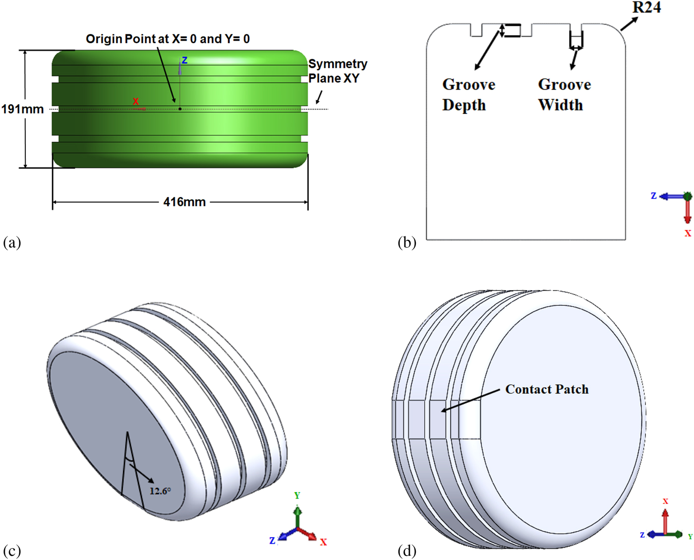
Fig. 1. (a) Tire model dimensions, origin axis, and symmetry plane. (b) Groove dimensions. (c) 3D tire model with longitudinal grooves. (d) Tire contact patch attached to road.
Table 1. The main dimensions of tire model

Computational domain
A computational domain (with x–y plane acting as a plane of symmetry and cutting the domain in half) is made as shown in Figure 2. The origin point, axis orientation, and symmetry plane are same for the computational domain as shown in Figure 1a. The dimensions of the computational domain (virtual wind tunnel) are set based on recommendation in the literature (Knowles, Reference Knowles2005; Lanfrit, Reference Lanfrit2005; Wang et al., Reference Wang, Burton, Herbst, Sheridan and Thompson2018). Walls of the domain are set far away from tire model and has no effect on the flow around the geometry. Upstream dimension is X 1/D = 5.5 and downstream dimension X 2/D = 10.5. Height of domain is Y 1/D = 7 and Y 2/D = 0. Width of domain is Z 1/D = 5 and Z 2/D = 5 where D is the diameter of the tire model. Based on these dimensions, the frontal area of the tire model is 0.65% of domain's frontal area in Y–Z plane. The accuracy of the results depends upon the ratio of frontal area of tire model to frontal area of the computational domain (Das et al., Reference Das, Tsubokura, Matsuuki, Oshima and Kitoh2013; Blocken and Toparlar, Reference Blocken and Toparlar2015; Collin et al., Reference Collin, Indinger and Müller2017; Haag et al., Reference Haag, Blacha and Indinger2017). The flow inlet and outlet definitions are given to front and back walls as shown in Figure 2.
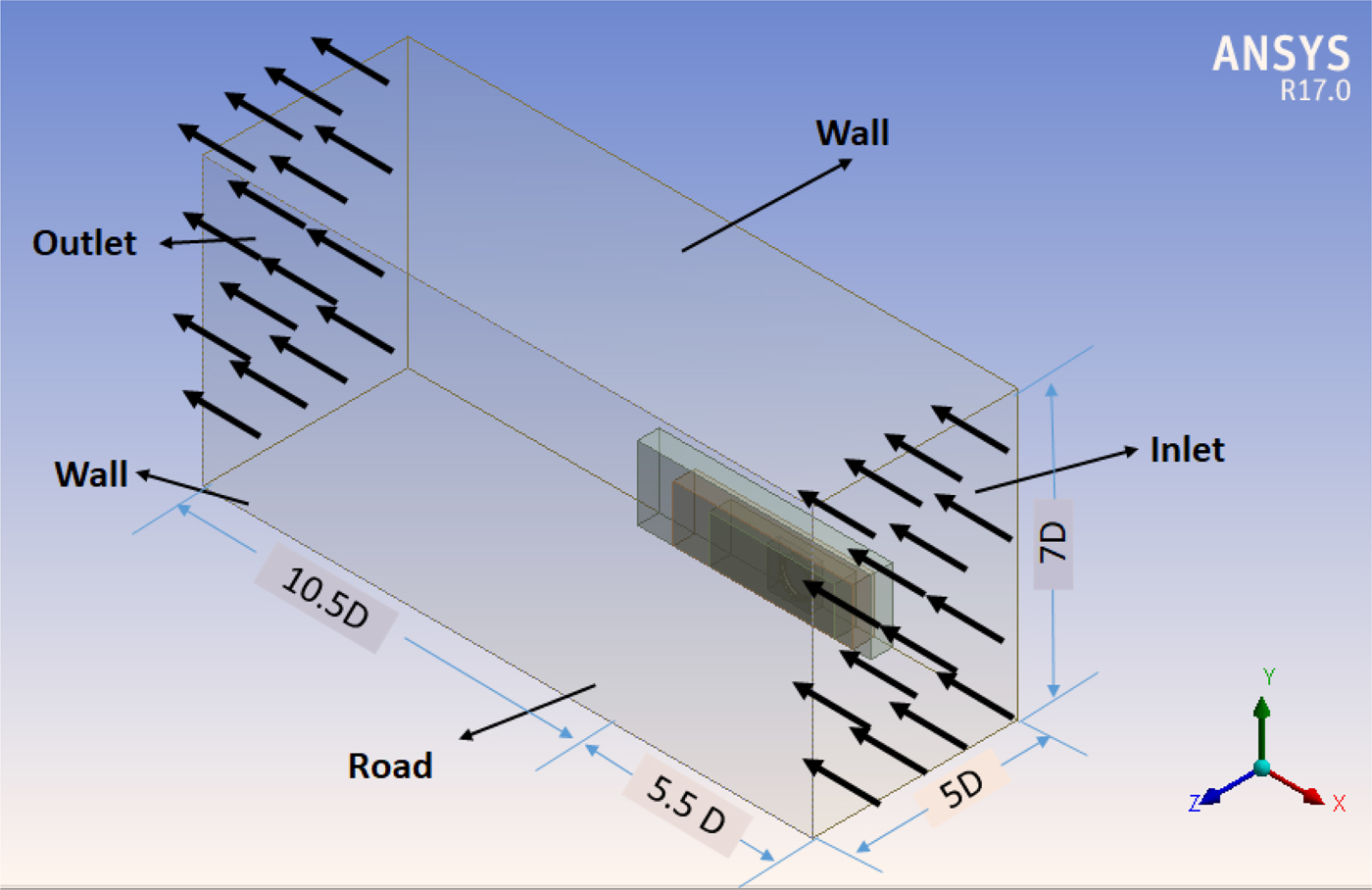
Fig. 2. Computational domain (virtual wind tunnel) for the computer-simulated experimentation.
Meshing
The meshing of the computational domain is made in Ansys meshing module using the hybrid meshing approach. In order to control the cell generation, refinement zones are introduced near the tire model (Strumolo and Babu, Reference Strumolo and Babu2000; Abohela et al., Reference Abohela, Hamza and Dudek2013). For mesh generation, automatic meshing algorithm approach is applied (Haag et al., Reference Haag, Blacha and Indinger2017). Tetrahedral cells are used to fill the domain including the region of refinement zones (Çengel, Reference Çengel2010). Inflation layers are developed on tire boundary and road surface to capture better flow characteristics (Grabowski et al., Reference Grabowski, Baier, Buchacz, Majzner and Sobek2015; Holder et al., Reference Holder, Malla and Gutmark2018; Wang et al., Reference Wang, Burton, Herbst, Sheridan and Thompson2018). Prism cells are used to construct the inflation layers. Contact patch is introduced between the tire geometry and road (Diasinos et al., Reference Diasinos, Barber and Doig2015; Haag et al., Reference Haag, Blacha and Indinger2017). A growth rate of 1.2 (20%) is set at all the interfacing zones so that adjacent cells grow gradually and the computation error is minimized (Ahmad et al., Reference Ahmad, Abo-Serie and Gaylard2010). The meshed computational domain along with the zoomed view of tire model in the computational domain and a zoomed view of inflation layer is shown in Figure 3a. The treatment of tire grooves and the meshed tire geometry before and after the computational domain is split into symmetrical halves that can be seen in Figure 3b.

Fig. 3. (a) Meshed computational domain, the zoomed view of tire model, and inflation layer at the interface of the tire model with immediate next zone of the computational domain. (b) The treatment of tire grooves before and after symmetrical halves.
A comprehensive mesh independence analysis is conducted for both our measures, that is, C d and C l. At the start of the mesh independence study, the total number of cells in the whole computational domain (the tire model, the road, the five refinement zones, and the rest of domain) were 1 million. The number of cells in the refinement zones are systematically increased by reducing the size of the cells to assess the percentage relative error in the computed values of C d and C l. The systematic increase in the number of cells was continued till the percentage relative error is reduced below 3% (Ahmad et al., Reference Ahmad, Abo-Serie and Gaylard2010; Diasinos et al., Reference Diasinos, Barber and Doig2015). The results with 8, 9, and 10 million cells in the mesh independence analysis showed that the percentage relative error for drag and lift was reduced to an acceptable range of below 2%. Further increase in the number of cells will lead to a high computational cost without any significant improvement in the computational accuracy. The final selected computational domain after the mesh independence analysis constituted 9 million cells with majority of the cells confined within the refinement zones.
Numerical model configuration
Results from Shih et al. (Reference Shih, Liou, Shabbir, Yang and Zhu1995) depict that the two-equation Realizable K-ε model is a robust model and it has the ability to accomplish high accuracy for rotating and separating flows. Both the rotating and the separating flow phenomena occur in our computer-simulated experiments. The comparison between different turbulence models on tire model is given by Diasinos et al. (Reference Diasinos, Barber and Doig2015). The Realizable K-ε RANS model is used to solve complex flows by different studies (Doig and Barber, Reference Doig and Barber2011; Blocken and Toparlar, Reference Blocken and Toparlar2015; Diasinos et al., Reference Diasinos, Barber and Doig2017). The significance of Unsteady Reynolds-averaged Navier–Stokes equations (URANS) cannot be undermined. However, previous research work has reported that steady-state incompressible RANS model can be used without compromising much accuracy (Hobeika et al., Reference Hobeika, Sebben and Landstrom2013; Vdovin et al., Reference Vdovin, Bonitz, Landstrom and Lofdahl2013; Heo et al., Reference Heo, Ju, Kim and Kim2014; Diasinos et al., Reference Diasinos, Barber and Doig2015). Furthermore, steady RANS has been reported as still being the most used and accepted approach in vehicle industry (Diasinos et al., Reference Diasinos, Barber and Doig2015). Therefore, steady-state analysis is conducted in this research work as this remains the preferred approach in academia and in industry (Defraeye et al., Reference Defraeye, Blocken, Koninckx, Hespel and Carmeliet2010; Diasinos et al., Reference Diasinos, Doig and Barber2014; Dang et al., Reference Dang, Gu and Chen2015; Diasinos et al., Reference Diasinos, Barber and Doig2017). The solution is set as implicit and a finite volume method is used to solve RANS equation (McManus and Zhang, Reference Mcmanus and Zhang2005). For pressure and velocity coupling, the coupled algorithm is used as it is more robust and performs well as compared with the segregated solution scheme (Hobeika et al., Reference Hobeika, Sebben and Landstrom2013; Ansys, Reference Ansys2016). Equations are discretized as first-order upwind scheme for the first 400 iterations so that the computational domain can be filled with numbers. First-order upwind scheme can converge in much less amount of time but is less accurate than the second-order upwind scheme. Therefore, after the first 400 iterations, the solution is further run with second-order upwind scheme till the results obtained meet the convergence criteria (McManus and Zhang, Reference Mcmanus and Zhang2005; Gérardin et al., Reference Gérardin, Gentric and Midoux2014). The solution is considered as converged when residual of energy terms reach the value of ≤10−6, residual of velocity (x, y, and z) reach the value of ≤10−8, and residual of continuity reach the value of ≤10−5 (Diasinos et al., Reference Diasinos, Barber and Doig2015). All other solver settings can be found in the guide lines of Ansys Fluent (Ansys, Reference Ansys2016).
Boundary conditions
The rotation of tire model is simulated by the moving wall approach (McManus and Zhang, Reference Mcmanus and Zhang2005). Turbulence intensity of the freestream is set to 0.2% (Watkins et al., Reference Watkins, Saunders and Hoffmann1995). A linear (translational velocity) is assigned to the inlet air flow (which is velocity inlet boundary) in negative “x” direction. An angular (rotational) velocity (ω z) is assigned to the tire in negative “z” direction, as shown in Figure 4a. At the outlet wall (which is pressure outlet boundary), a gauge pressure of zero is set. The road is specified with a no slip boundary condition to simulate the contact between the road and the tire (McManus and Zhang, Reference Mcmanus and Zhang2005). The result containing pressure contour plot on the tire model for a selected computer-simulated experiment is shown in Figure 4b.

Fig. 4. (a) The rotational motion of tire (ω z) and direction of air flow. (b) The pressure contour plot on tire model.
Process modeling
The design of experiments
The basic level of comparison between the slick and the grooved tire's coefficients of drag and lift has been reported in the previous research work (Hobeika et al., Reference Hobeika, Sebben and Landstrom2013; Leśniewicz et al., Reference Leśniewicz, Kulak and Karczewski2014). But there is a need of a detailed study which can give answers to questions like how lift and drag are affected by changing groove depth or groove width. Furthermore, the effect of temperature and velocity on coefficients of drag and coefficients of lift need to be investigated alongside the varying groove width and groove depth.
A full factorial computer-simulated experimental study answering the aforementioned questions is presented in this research work. The main geometry of tire remains unchanged. Four control variables are considered, that is, groove depth (x 1), groove width (x 2), temperature (x 3), and freestream velocity (x 4), maintaining all other conditions constant. The full factorial design of experiments was constructed based on seven levels of groove depth, seven levels of groove width, two levels of temperature, and four levels of velocity. The configuration of the input space of the full factorial design of experiment is shown in Table 2. The design constituted 392 computer-simulated experiments. C d and C l are two output variables.
Table 2. Variables and their corresponding levels for the full factorial design of experiment

a (Leśniewicz et al., Reference Leśniewicz, Kulak and Karczewski2016; Dieselnet, 2018, Maxxis, 2018).
Artificial neural network
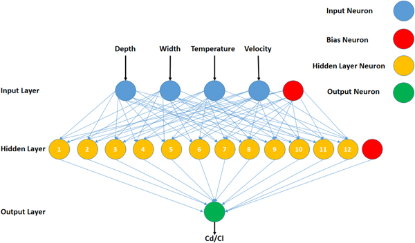
Artificial neural networks (ANN) are well known for their ability to map any extent of non-linearity in the data (Uddin et al., Reference Uddin, Ziemer, Sun, Zeid and Kamarthi2013; Uddin et al., Reference Uddin, Ziemer, Zeid and Kamarthi2015a). Therefore, gradient descent back propagation algorithm-based multi-layer perceptron (MLP)-type ANN are deployed as process models for the computer-simulated design of experiments shown in Table 2. The variables x 1, x 2, x 3, and x 4 are fed to ANN as inputs and variables C d and C l are fed as outputs for the neural network training, testing, and validation. The configuration of 4-12-1 (input-hidden-output layer neurons) is employed in the development of MLPs. A learning rate of 0.01 is set for the MLP training. A tangent hyperbolic function is deployed for the forward movement of signal at the nodes of hidden and output layers and gradient decent algorithm is applied for error convergence. The networks are set to train for 10,000 epochs and stopping criterion of 0.0000001 as change in error or no change in error for 2,000 epochs are set. A split of 80%, 10%, and 10% is set for training, testing, and validation of the MLPs. Figure 5 presents a generic diagram of MLPs employed in our study. The MLP-based ANN configuration is summarized in Table 3.
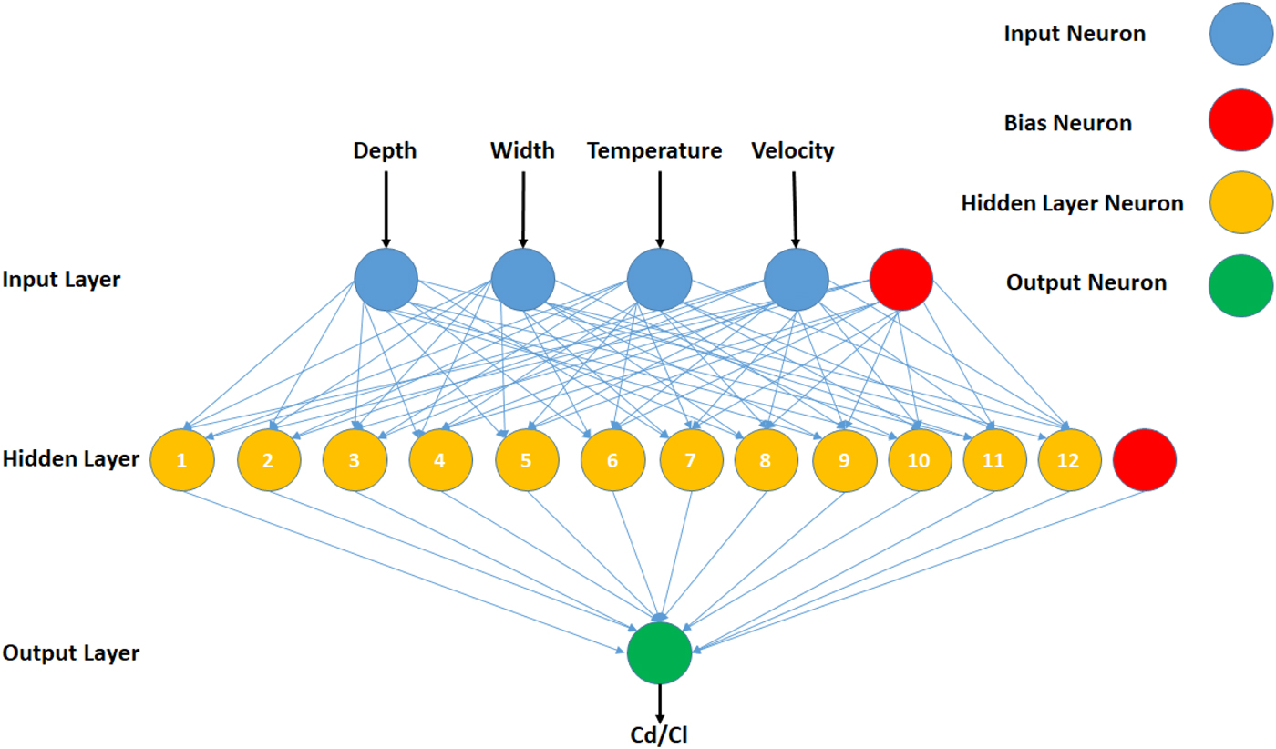
Fig. 5. Generic diagram of MLPs for C d and C l.
Table 3. Summary of ANN configuration
Monte-Carlo experimentation
Monte-Carlo experiments are used to study the causal relationship between the control variables and the output variables using the trained MLP computer models (Uddin et al., Reference Uddin, Ziemer, Sun, Zeid and Kamarthi2013, Reference Uddin, Ziemer, Zeid and Kamarthi2015a, Reference Uddin, Ziemer, Zeid and Kamarthi2015b). In this research work, three types of MLP-assisted Monte-Carlo analyses are being presented, that is, sensitivity analysis, significance analysis, and paired interaction analysis. The details of Monte-Carlo experiments for sensitivity, significance, and paired interaction analyses are given below:
Monte-Carlo experiment 1: factor-wise sensitivity analysis
(1) Four control variables are selected in this experiment, that is, groove depth, groove width, temperature, and velocity. Let x i represent a control variable where i = 1,2,3,4. x 1 = groove depth, x 2 = groove width, x 3 = temperature, and x 4 = velocity. Two output variables which are performance variables are represented by y 1 and y 2.
(2) x i is varied at regular intervals between its minimum value and its maximum value and n experimental treatments are created. Each varied value of x i is represented by x ik where k = 1,2,3 …, n. All other control variables are represented by x j where j = 1,2,3,4 and j ≠ i are kept constant at their respective mid values. The k th input vector for first control variable can be represented as (x 1k, x 2mid, x 3mid, x 4mid) and respective output vector is represented by y 1k and y 2k.
(3) M replications are created for each treatment of k. For each subset of M replications, x ik is kept constant while all other control variables (x j where j ≠ i) are perturbed about their mean value. The perturbations are created based on a Gaussian noise with mean equal to zero and standard deviation equal to 1% of x jmin and added to x jmid of each control variable x j.
(4) The ANN-based computer-simulated model is used to find the response of x ik for n experimental treatments where each experimental treatment constitutes M replications. The responses are obtained in the form of y 1ikm and y 2ikm where k = 1,2,3,…,n and m = 1,2,3,…,M. A Gaussian noise is added to the obtained responses to account for the error in ANN-based computer-simulated model. This Gaussian noise is obtained from N(μ ne, σ ne). The μ ne and σ ne are mean and standard deviation of the ANN-based computer-simulated model's prediction error.
(5) From each y 1ikm and y 2ikm where m = 1,2,3,…,M mean (μ 1ik and μ 2ik respectively) and standard deviation (σ 1ik and σ 2ik, respectively) are calculated.
(6) The mean, upper control limit (UCL), and lower control limit (LCL) trend lines for y 1 are obtained from (μ 1ik), (μ 1ik + 3σ 1ik), and (μ 1ik – 3σ 1ik), respectively. Similarly, the counterparts of y 2 are used for its mean, UCL, and LCL trend lines.
Monte-Carlo experiment 2: significance analysis
Repeat the steps from 1 to 5 as discussed in “Monte-Carlo experiment 1: factor-wise sensitivity analysis” with an exception in step number 3 which is as follows:
x ik is kept constant for each k value while generating M replications of each kth treatment. All control variables x j are randomly varied between their respective minimum and maximum values for the whole data set.
Monte-Carlo experiment 2: paired interaction analysis
Repeat the steps from 1 to 5 as discussed in “Monte-Carlo experiment 1: factor-wise sensitivity analysis” with an exception in step number 3 which is as follows:
x ik is kept constant for each k value while generating M replications of each kth treatment. Its pair control variable x j is randomly varied between its minimum and maximum value and remaining control variables x j are kept at their respective middle value for whole data set.
Results and discussion
The results presented in this section are based on computer-simulated experiments, MLP-based neural network process model, and Monte-Carlo analysis.
Artificial neural network results
The data set constituting 392 data points each representing four control variables and two output variables, that is, C d and C l is used to prepare neural network computer models. Two separate MLPs are trained for C d and C l. The effectiveness of the neural network computer model was decided based on the goodness-of-fit criteria (the R 2 for training data subset, the R 2 for testing data subset, and the R 2 for validation data subset). The R 2 values (in case of C d) for training, testing, and validation are 0.922, 0.946, and 0.928, respectively. The R 2 values (in case of C l) for training, testing, and validation are 0.962, 0.979, and 0.976, respectively.
The trend line of error reduction in MLP with number of training epochs is shown in Figure 6. Both C d neural network model shown in Figure 6a and C l neural network model shown in Figure 6b present a steady error convergence for 10,000 epochs. The training and testing error of the MLP decrease significantly for first 4000 epochs after which a steady decrease is observed. Therefore, if both the networks are further trained, they will only decrease error marginally.

Fig. 6. (a) Training graph for (MLP 4-12-1) drag coefficient case. (b) Training graph for (MLP 4-12-1) lift coefficient case.
Factor-wise sensitivity and significance analysis
In this section, the sensitivity and significance analyses present the behavior and importance of a control variable with respect to co-responding output variable. The sensitivity analysis studies the trend of a particular output variable against a control variable by varying the concerned control variable at regular intervals and keeping all other variables at their mid values. Further in order to test the robustness of the neural network computer models, 10 replications of each data points are created by adding 1% Gaussian noise. The significance analysis studies the role played by a particular variable in determining an output variable by changing concerned control variable at regular intervals and all other control variables randomly between their minimum and maximum values, respectively. The graph of sensitivity trend of a particular variable can be assessed based on the gradient of its mean trend line. In case of significance trend; if the shape of the corresponding sensitivity trend is retained in significance graph (mean, UCL, and LCL) of a particular variable, then that particular variable has a stronger causal relationship with output variable. Furthermore, the extent of widening of the confidence interval of a particular variable in its significance trend reflects its strength in comparison with its peer control variables.
Groove depth
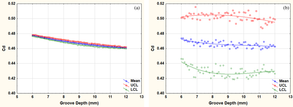
The sensitivity trend of C d with respect to the groove depth is shown in Figure 7a. A steady and significant reduction (~3.2%) in C d can be achieved by increasing the groove depth up to 11 mm. However, increasing the groove depth beyond that point would not contribute any significant saving in the C d.

Fig. 7. (a) C d versus groove depth in sensitivity analysis and (b) C d versus groove depth in significance analysis.
The significance trend of C d with respect to the groove depth is shown in Figure 7b. The reduction gradient of the significance trend of C d between the groove depth up to 11 mm is ~2.2%. The random variations in the peer control variables of groove depth (groove width, temperature, and velocity) appear to significantly reduce the gradient of the trend. Moreover, the confidence interval, that is, the gap between UCL and LCL widens. This reinforces the possibility of some other control variables being more significant than groove depth.
The sensitivity trend of C l with respect to the groove depth is shown in Figure 8a. A steady and significant reduction (~21%) in C l can be achieved by increasing the depth of groove up to 11 mm. However, increasing the groove depth beyond that point would not contribute any significant reduction in the C l. This behavior of C l with respect to groove depth is identical to the corresponding behavior of C d with respect to groove depth.

Fig. 8. (a) C l versus groove depth in sensitivity analysis and (b) C l versus groove depth in significance analysis.
The significance trend of C l with respect to the groove depth is shown in Figure 8b. The random variations in the peer control variables of groove depth (groove width, temperature, and velocity) appear to significantly reduce the gradient of the trend. The confidence interval, that is, the gap between UCL and LCL widens as the groove depth increases. Again the widening of the UCL–LCL gap at higher values of groove depth for C l is identical to the corresponding behavior of the significance trend of C d.
Groove width
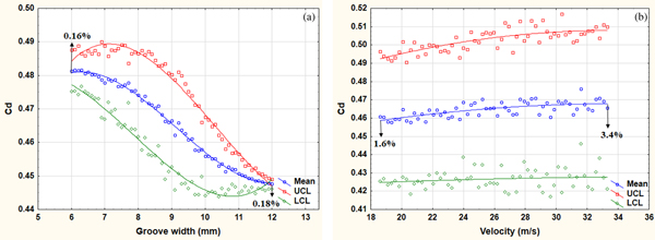
The sensitivity trend of Cd with respect to the groove width is shown in Figure 9a. A steady and significant reduction (~6.8%) in C d can be achieved by increasing the width of groove from 7 to 12 mm. The sensitivity trend suggests that by increasing the groove width beyond 12 mm may further reduce C d and contribute in further savings.

Fig. 9. (a) C d versus groove width in sensitivity analysis and (b) C d versus groove width in significance analysis.
The significance trend of C d with respect to the groove width is shown in Figure 9b. The reduction gradient of the significance trend of C d between the groove width of 7–12 mm is ~5.4%. The random variations in the peer control variables of groove width (groove depth, temperature, and velocity) appear to have almost no effect on the gradient of the trend. The gap between UCL and LCL tends to retain its width from mean trend line throughout the range, that is, from 6 to 12 mm. The comparison between Figures 7b, 9b confirms that the groove width is significantly stronger variable.
The sensitivity trend of C l with respect to the groove width is shown in Figure 10a. A steady and significant reduction (~41%) in C l can be achieved by increasing the width of groove from 6 to 12 mm. The sensitivity trend suggests that by increasing the groove width beyond 12 mm may further reduce C l.

Fig. 10. (a) C l versus groove width in sensitivity analysis and (b) C l versus groove width in significance analysis.
The significance trend of C l with respect to the groove width is shown in Figure 10b. The random variations in the peer control variables of groove width (groove depth, temperature, and velocity) appear to have no effect on the gradient of the trend. The gap between UCL and LCL tends to retain its width with mean throughout the experimental range. The comparison between Figures 8b, 10b also confirms that the groove width is almost twice as significant variable than the groove depth.
Temperature
The sensitivity trend of C d with respect to the temperature is shown in Figure 11a. A nearly constant reduction (~0.7%) in C d can be observed by increasing the temperature between 15°C and 40°C. The trend also depicts that increasing the temperature to the range of 50°C–55°C may only reduce the C d to 1%.
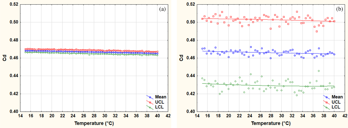
Fig. 11. (a) C d versus surrounding temperature in sensitivity analysis and (b) C d versus surrounding temperature in significance analysis.
The significance trend of C d with respect to the temperature is shown in Figure 11b. The gradient of the mean line in Figure 11b between 15°C and 40°C is ~1.3%. The random variations in the peer control variables of temperature (groove depth, groove width, and velocity) appear to have no effect on the gradient of the trend. The gap between upper UCL and LCL widens as the temperature increases. Therefore, irrespective of the weak gradient of temperature, its impact on the C d remains.
The sensitivity trend of C l with respect to the temperature is shown in Figure 12a. A steady reduction (~4.2%) in C d can be observed by increasing the temperature.

Fig. 12. (a) C l versus surrounding temperature in sensitivity analysis and (b) C l versus surrounding temperature in significance analysis.
The significance trend of C l with respect to the temperature is shown in Figure 12b. The gradient of the mean line in Figure 12b between 15°C and 40°C is ~10%. The random variations in the peer control variables of temperature (groove depth, groove width, and velocity) appear to have no effect on the gradient of the trend. The gap between upper UCL and LCL widens as the temperature increases. Therefore, irrespective of the weak gradient of temperature, its impact on the C l remains.
Velocity
The sensitivity trend of C d with respect to the velocity is shown in Figure 13a. A steady and significant increase (~3.9%) in C d is observed by increasing the velocity. The sensitivity trend suggests that by increasing the velocity beyond 33 m/s, a further increase C d can be expected.

Fig. 13. (a) C d versus tire velocity in sensitivity analysis and (b) C d versus tire velocity in significance analysis.
The significance trend of C d with respect to the velocity is shown in Figure 13b. The gradient increase of the significance trend of C d between the velocity values 18.6 and 33.3 m/s is ~2.1%. The random variations in the peer control variables of velocity (groove depth, temperature, and velocity) appear to have some effect on the gradient of the trend.
The sensitivity trend of C l with respect to the velocity is shown in Figure 14a. A steady and significant increase (~35%) in C l is observed by increasing the velocity. The sensitivity trend suggests that by increasing the velocity beyond 33 m/s, a further increase C l can be expected.

Fig. 14. (a) C l versus tire velocity in sensitivity analysis and (b) C l versus tire velocity in significance analysis.
The significance trend of C l with respect to the velocity is shown in Figure 14b. The reduction gradient of the significance trend of C d between the velocity values 18.6 and 33.3 m/s is ~12% which is the half of the gradient of the significance trend. The random variations in the peer control variables of velocity (groove depth, temperature, and velocity) appear to have a significant effect on the gradient of the trend.
The sensitivity and the significance analyses give insightful information about the aerodynamics of tire model. Hobeika et al. (Reference Hobeika, Sebben and Landstrom2013) studied tread style as a design parameter and showed that treads are an important factor in aerodynamics of tires. A more in-depth study (how tread dimension effect aerodynamics of tire) is presented in this research work. These results show that the coefficient of drag and coefficient of lift vary with the change in velocity as confirmed by previous research (Vdovin, Reference Vdovin2015; Leśniewicz et al., Reference Leśniewicz, Kulak and Karczewski2016). The reduction in C d is expected to reduce the overall contribution of tire geometry on vehicle drag and in turn on fuel consumption. The reduction in C l is expected to reduce the overall contribution of tire geometry to vehicle stability and in turn better steering and road safety. The comparison of significance among the control variables is decided based on a detailed study of sensitivity analysis and significance analysis. A summary of approximate percentage change of output variables with respect to the input variables in sensitivity analysis is given in Table 4. The comparison between Figures 7b, 9b, 11b, 13b confirms that the order of significance of the control variables with respect to coefficient of drag is (a) groove width, (b) velocity, (c) groove depth, and (d) temperature. The comparison between Figures 8b, 10b, 12b, 14b confirms that the order of significance of the control variables with respect to coefficient of lift is (a) groove width, (b) velocity, (c) groove depth, and (d) temperature. Furthermore, in most of the previously reported literature, C d and C l are considered to be constant at all velocities while testing for variables like tire grooves, etc. This research reveals that the velocity can have a significant impact on C d and C l, that is, 4% and 35%, respectively, per tire. Therefore, it may not be considered insignificant for studies relating to contribution of tires in aerodynamic drag and steering stability.
Table 4. Summary of percentage approximation of changes in C d and C l values in sensitivity trends

Paired interaction analysis
The paired interaction analyses of important pairs are discussed in this section. In case of paired interaction trend; if the trend lines of the particular variable's corresponding sensitivity trend are unchanged in paired interaction graph, then its paired variable has no effect on the behavior of that particular variable. In this paired interaction study, a qualitative assessment in the shift of trend lines is made by considering the edges of both paired interaction graphs and its corresponding sensitivity graph. An approximate percentage change in the value of edges is calculated and mentioned to understand the extent of interaction between the concerned interacting variable and the corresponding output variable (C d and C l).
Groove depth and groove width
The paired interaction analyses between groove depth and groove width, with respect to C d and C l, respectively, are shown in Figures 15, 16. The percentage increase or decrease values at the extreme ends shown are calculated based on the corresponding values from sensitivity trends in Figures 7a, 8a, 9a, 10a.

Fig. 15. Paired interaction analysis: (a) C d versus groove depth with randomly varying groove width and (b) C d versus groove depth with randomly varying groove depth.
Fig. 16. Paired interaction analysis: (a) C l versus groove depth with randomly varying groove width and (b) C l versus groove depth with randomly varying groove depth.
Nearly insignificant increase of 0.3% and 0.7% at the edges of Figure 15b reveal that there is almost no interactive effect of groove depth on the strong dependence of tire aerodynamic drag (Cd) on groove width. However, a significant ~11% increase at the higher end of Figure 16b is observed. This shows strong interaction between the control variables groove depth and groove width in terms of C l; consequently, having significant possible impact on stability. The air entrapped between the groove of the tire and the road acts as an air beam as shown in Figure 17. This entrapped air acts like a typical beam as its impact on C l (stability) increases as the groove depth/the air beam height increases. A similar kind of higher strength behavior along the greater cross-sectional dimension of general beams is observed in engineering applications which is explained by the section modulus in beam theory.
Fig. 17. Section of single groove forming air beam in contact with the road surface.
Groove width and velocity
The paired interaction analyses between groove width and velocity, with respect to C d and C l, respectively, are shown in Figures 18, 19. The percentage increase or decrease values at the extreme ends shown are calculated based on the corresponding values from sensitivity trends in Figures 9a, 10a, 13a, 14a.

Fig. 18. Paired interaction analysis: (a) C d versus groove width with randomly varying velocity and (b) C d versus velocity with randomly varying groove width.

Fig. 19. Paired interaction analysis: (a) C l versus groove width with randomly varying velocity and (b) C l versus velocity with randomly varying groove width.
Again, the insignificant change of 0.16% and 0.18% at the edges of Figure 18a and 1.4% and 1.2% at the edges of Figure 19a reveals that there is almost no interactive effect of velocity on the strong dependence of tire aerodynamic drag (C d) and aerodynamic lift (C l) on groove width. However, a significant 1.6%–3.4% and 9.3%–10% decrease at the extreme ends of Figures 18b, 19b is observed. This shows strong interaction between the control variables groove width and velocity in terms of C d and C l; consequently, having significant impact on stability.
Conclusion
(i) Neural networks offer a very effective model to study any non-linearity in causal relationships of tire aerodynamics.
(ii) The Monte-Carlo analysis on neural network process models can help conduct the parametric analysis.
(iii) The tight confidence interval of the sensitivity trends reinforces the robustness of the neural network model.
(iv) The order of the significance of the control variables for both C d and C l is groove width > velocity > groove depth > temperature. Therefore, the mixing of design parameters and operational parameters is imperative for CFD studies related to tire aerodynamics.
(v) This research also emphasizes that at different velocities the coefficient of drag and the coefficient of lift cannot be considered as constant.
(vi) Increasing the groove depth can help reduce the C d by ~4% and C l by ~20%. However, the possibility of reduction in the coefficient of drag and coefficient of lift is very low after 11 mm.
(vii) Increasing the groove width can help reduce the C d by ~7% and C l by ~40%. The possibility of further reduction in C d appears to diminish beyond the range of 12–13 mm. However, the possibility of reduction in the C l is possible beyond that range and may be considered for investigation in future research.
(viii) The change in design parameters (groove depth and groove width) has a considerable impact on both drag and lift and in turn can have an impact on fuel savings and stability, respectively.
(ix) The negligible significance of the control variable the temperature reveals that the results may be considered independent of the effect of seasonality.
(x) The groove width and the groove depth both have proven to be a strongly interacting pair of control variables with respect to both C d and C l.
(xi) The air trapped between the tire groove and the road acts as a beam and exhibits the behavior similar to the concept of section modulus in beam theory.
(xii) The effect of cross wind, different groove types, and number of grooves still needs to be investigated. This work is limited to straight air flow (entering air flow is 90° to z-axis) and with only three longitudinal grooves.
Future work
For further research, design parameters and operational parameters of an isolated tires with different configurations of treads especially, longitudinal grooves with shoulder grooves may be studied. A similar kind of study may be conducted for the inlet air flow from a range of directions such that the angle between the inlet air and z-axis is not equal to 90°.The computer-simulated experiments, MLP-based neural network process model, and Monte-Carlo analysis coupling may also be used to study variable behavior in other components of cars like spoilers, under-tray, and diffusers, etc. The change in C d and C l suggest that a similar type of study should be conducted for acoustic analysis and aquaplaning of an isolated tire as well as acoustic analysis and aquaplaning for tires in cars.
Ghulam Moeen Uddin is an Assistant Professor at the Mechanical Engineering Department, University of Engineering and Technology, Lahore. His area of expertise includes machine learning and its applications, tribology, manufacturing process development for semiconductor devices on wide band gap substrates, UHV thin film growth processing and characterization, and wet and dry etching-based surface processing, and chemical and structural characterization. He has published research papers in the areas of surface processing, UHV thin film growth for metal oxides, and developing process control models for optimizing nano-manufacturing processes for transfer from the laboratory to high-volume manufacturing.
Syed Muhammad Arafat is a PhD candidate at the Mechanical Engineering Department, University of Engineering and Technology, Lahore. His research interests include manufacturing process development, design optimization, computational fluid dynamics, and artificial intelligence.
Ali Hussain Kazim is an Assistant Professor at the Mechanical Engineering Department, University of Engineering and Technology, Lahore. His research interests are in the fields of thermodynamics and CFD.
Muhammad Farhan is an Assistant Professor at the Mechanical Engineering Department, University of Engineering and Technology, Lahore. His research interests include computational fluid dynamics and HVAC.
Sajawal Gul Niazi is a graduate student at the Mechanical Engineering Department, University of Engineering and Technology, Lahore. His research interests include computational fluid dynamics and machine learning.
Nasir Hayat is a Professor and currently working as Chairman at the Mechanical Engineering Department, University of Engineering and Technology, Lahore. He holds the PhD degree from Toyohashi University of Technology, Japan. His research interests include manufacturing systems, engineering economic analysis, operational research, and application of artificial intelligence in manufacturing.
Ibrahim Zeid is a Professor of Mechanical and Industrial Engineering at Northeastern University. His research interests include database and information systems in manufacturing, the use of mobile agents to facilitate information access in manufacturing environments, developing XML-based algorithms for mass customization, and developing Java-based and web-based systems for disassembly analysis. Currently his research is focused on scalable nano-manufacturing and engineering education. He has published over 200 papers and secured research grants worth over $3 million.
Sagar Kamarthi is a Professor of Mechanical and Industrial Engineering at Northeastern University. His research interests are in the areas of advanced manufacturing, scalable nano-manufacturing, machine learning, process monitoring and diagnosis, and intelligent sensors/sensor integration. He has published more than 160 articles in internationally reputed journals and has secured several grants from the the National Science Foundation. He has secured research grants worth over $3.5 million. His current research focuses on scalable manufacturing of nano-enabled products.