


1. Introduction
The dissolution of a solid in a liquid is ubiquitous in nature and industry such as erosion, rock fractures, melting, etc. The dissolution rate and periodic pattern formation of a soluble solid body are determined by the complex mass transfer and reaction rate (Wagner Reference Wagner1949; Cohen et al. Reference Cohen, Berhanu, Derr and du Pont2016; Guérin et al. Reference Guérin, Derr, du Pont and Berhanu2020; Hu et al. Reference Hu, Wang, Yang, Xiao, Chen and Zhou2021; Wang et al. Reference Wang, Hu, Yang, Zhou, Chen and Zhou2022). Specifically, when a salt is dissolving in a liquid, dynamic mass transport phenomena around the dissolving solid exist, changing the shape of the solid body of the salt. Huang et al. (Reference Huang, Nicholas, Moore and Ristroph2015) remarkably demonstrated the recession of a dissolving solid in a high-speed laminar flow and the effect of the solid body geometry on the dissolution process. Accordingly, to predict the dissolution rate and pattern formation successfully, several factors, including the flow and body geometry, must be considered in addition to the mass transfer on the dissolving surface (Kimura, Tanaka & Sukegawa Reference Kimura, Tanaka and Sukegawa1990; Sullivan, Liu & Ecke Reference Sullivan, Liu and Ecke1996; Huang et al. Reference Huang, Nicholas, Moore and Ristroph2015; Nakouzi, Goldstein & Steinbock Reference Nakouzi, Goldstein and Steinbock2015; Philippi et al. Reference Philippi, Berhanu, Derr and du Pont2019; Cohen et al. Reference Cohen, Berhanu, Derr and du Pont2020). The effects of gravitational instability on the dissolution rate and pattern formation under a stationary solvent condition have been studied, but only in a limited manner.
Nakouzi et al. (Reference Nakouzi, Goldstein and Steinbock2015) showed that a vertical water-soluble cylinder object evolves into a paraboloid shape due to the inevitable density-driven flow in the vertical geometry, which experiences non-uniform flux. Later, Pegler & Davies Wykes (Reference Pegler and Davies Wykes2020) analysed theoretically and experimentally the effect of stable laminar natural convective flow on the shape evolution of vertical conic solid bodies. In addition, Davies Wykes et al. (Reference Davis Wykes, Huang, Hajjar and Ristroph2018) experimentally examined the shape dynamics of a dissolving body in the presence of the buoyancy driven self-generated flows. In their experiments, for various quasi-two-dimensional and three-dimensional (3-D) axisymmetric solids, the dissolution of the underside is strongly affected by the gravitational instabilities generated by the unstable density profile near the surface and, therefore, on the underside of a partially dissolved wedge, small-scale roughness is observed. In the context of ultra-sharp pinnacle formation, Huang et al. (Reference Huang, Tong, Shelley and Ristroph2020) experimentally and theoretically studied the effects of thermodynamics (Joule–Thompson effect) and hydrodynamics (natural convective flow) on the formation of pinnacles. According to their analysis, the hydrodynamic factor is important in the formation of ultra-sharp pinnacles.
In an inclined geometry, a parallel groove-type dissolution pattern forms at the surface of an initially flat soluble material due to a forced convective water flow (Guérin et al. Reference Guérin, Derr, du Pont and Berhanu2020). Cohen et al. (Reference Cohen, Berhanu, Derr and du Pont2020) studied the effect of a natural convective flow on the dissolution rate of an inclined solid block and pattern formation on the dissolving surface, finding that parallel stripes form beyond a certain length from the block end. Over time, these stripes cross and evolve into scallops that propagate upstream. Meanwhile, in a horizontal geometry, the formation of a dissolution pattern is affected by gravitational instability in a different manner. Sullivan et al. (Reference Sullivan, Liu and Ecke1996) experimentally visualized the dissolution of horizontal crystal bodies of NaCl, KBr and KCl in aqueous solutions. The dissolution rate and surface profile were compared with theoretical predictions in terms of Howard's (Reference Howard1966) boundary-layer instability model and Foster's (Reference Foster1968) linear stability. In an analysis with the boundary-layer instability model, the turbulent mass transfer rate was assumed to be closely related to the stability of the fluid layer. It was found that the wavelength of the dissolution pattern is significantly affected by the concentration gradient near the surface. Philippi et al. (Reference Philippi, Berhanu, Derr and du Pont2019) specifically identified the effects of dissolution-driven flow instability by defining the sequence of the dynamic transport phenomena around a solid body with three regimes: (i) one that was diffusive, (ii) one with the growth of instability and (iii) one that featured the emission of a plume, termed a quasi-stationary regime. Similar to the work by Sullivan et al. (Reference Sullivan, Liu and Ecke1996), Philippi et al. (Reference Philippi, Berhanu, Derr and du Pont2019) introduced a boundary-layer instability model in the quasi-stationary regime and linked the stability of the liquid layer to the mass transfer rate. Under the assumption of high mass transfer rates in the turbulent natural convection regime (Sullivan et al. Reference Sullivan, Liu and Ecke1996) and the quasi-stationary regime (Philippi et al. Reference Philippi, Berhanu, Derr and du Pont2019), they discussed the effects of the dissolution reaction on the surface on the onset of gravitational instability during dissolution and proposed several scaling relationships and compared these outcomes with experimental results. In addition, under the static assumption that the movement of the solid interface is much slower than the dissolution-driven convective motion, Philippi et al. (Reference Philippi, Berhanu, Derr and du Pont2019) and Berhanu et al. (Reference Berhanu, Philippi, du Pont and Derr2021) conducted nonlinear numerical simulations and a linear stability analysis of dissolution, respectively. Due to such a simplification, they could not simulate the temporal evolution of the interface position, i.e. pattern formation by dissolution-enhanced convective motion. Hence, none of the analyses considering realistic moving boundary conditions are applicable to simulate the dissolution process. Thus, while fluid flows are known to promote the dissolution of materials, such processes are poorly understood due to the coupled dynamics of the flow and the receding surface.
In this study, considering a moving interfacial boundary on a dissolving solid, the effects of dissolution on the onset of buoyancy-driven gravitational instability are coupled to simulate the dissolution of a horizontal salt body using linear stability theory and a numerical simulation. According to the dissolution regimes (i) and (ii) defined by Philippi et al. (Reference Philippi, Berhanu, Derr and du Pont2019), the effect of gravitational instability on the interfacial pattern formation on a dissolving surface is systemically studied. To simulate the growth of instability, a two-dimensional (2-D) nonlinear analysis is conducted using the commercial finite element method solver COMSOL Multiphysics (2019). As a case study, the dissolution of NaCl salt in water is simulated. Furthermore, the dissolution-driven interfacial pattern formation on a dissolving salt surface is visualized by fully 3-D numerical simulations. The effects of gravitational instability on the dissolution rate and pattern formation are demonstrated successfully. The present study will provide basic tools with which to predict the dissolution rate and to understand the dissolution-driven pattern formation process during the dissolution of a horizontal salt in a stationary solvent.
2. Governing equations and base fields
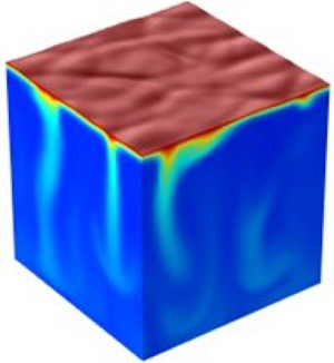
The system considered here is that of a horizontal salt body floating on top of a liquid with the initial liquid thickness of d and the initial concentration of solute in the liquid of  ${C_r}$. The schematic diagram of the system is shown in figure 1. Initially, the liquid is bounded by a flat solid salt. As time goes on $(t \ge 0)$, the solid salt dissolves in liquid at the solid salt–liquid interface until ${C_r}$ is lower than the saturation concentration, ${C_{sat}}$. In the meantime, the position of the interface moves upward until ${C_r} = {C_{sat}}$. In a binary mixture such as aqueous solution of salt, a linear relation between the density $\rho $ and mass concentration of solute C in the solution has been assumed (Philippi et al. Reference Philippi, Berhanu, Derr and du Pont2019). Under this assumption, the density of solution can be expressed as
 \begin{equation}\rho = {\rho _r} + \beta C,\end{equation}
where  ${\rho _r}$ is the density of pure solvent and $\beta \{ = ({\rho _{sat}} - {\rho _r})/{C_{sat}}\} $ is the densification coefficient. The concentration gradient driven by the salt dissolution makes the system unstable and convective motion will begin in a certain time period if the dissolution rate of salt is faster than the diffusive transport rate of dissolved salt. Considering sufficiently dilute concentrations of solute, we use the Boussinesq approximation, which consists of treating the liquid density as constant in all terms in the equations of motions except the one in the gravity force (Chandrasekhar Reference Chandrasekhar1961). The flow is then incompressible. By assuming that the liquid is a Newtonian fluid and the variation of temperature of the liquid can be neglected (Sullivan et al. Reference Sullivan, Liu and Ecke1996), the governing equations of flow and concentration fields are expressed as
 \begin{gather}\boldsymbol{\nabla }\boldsymbol{\cdot }\boldsymbol{U} = 0,\end{gather}
 \begin{gather}{\rho _r}\left\{ {\frac{\partial }{{\partial t}} + \boldsymbol{U}\boldsymbol{\cdot }\boldsymbol{\nabla }} \right\}\boldsymbol{U} =- \boldsymbol{\nabla }P + \boldsymbol{\nabla }\boldsymbol{\cdot }\{ \mu \boldsymbol{\nabla }\boldsymbol{U} + \mu {(\boldsymbol{\nabla }\boldsymbol{U})^T}\} + \beta C\boldsymbol{g},\end{gather}
 \begin{gather}\frac{{\partial C}}{{\partial t}} =- \boldsymbol{\nabla }\boldsymbol{\cdot }\boldsymbol{N},\end{gather}
 \begin{gather}\boldsymbol{N} =- \mathrm{{\mathcal{D}}}\boldsymbol{\nabla }C + C\boldsymbol{U},\end{gather}
 \begin{gather}\mu = \mu _{r} \exp(\gamma (C - C_{r})).\end{gather}
Here,  $\boldsymbol{U}( = \boldsymbol{i}U + \boldsymbol{j}V + \boldsymbol{k}W)$, P, $\boldsymbol{g}$, $\mu $, $C$,
$C$,  $\gamma$ and $\mathrm{{\mathcal{D}}}$ represent the velocity vector, the pressure, the gravitational acceleration, the viscosity, the mass concentration, the viscosity-variation parameter and the diffusivity, respectively. The variation of viscosity depending on concentration is modelled by (2.5), which has been widely used in related fields (Nijjer, Hewitt & Neufeld Reference Nijjer, Hewitt and Neufeld2018; Kim et al. Reference Kim, Pramanik, Sharma and Mishra2021). The given initial and boundary conditions are
 \begin{gather}\boldsymbol{U} = 0\quad \textrm{and}\quad C = {C_r}\;\textrm{at}\;t = 0,\end{gather}
 \begin{gather}\boldsymbol{U} = {\boldsymbol{U}_L}\quad \textrm{and}\quad C = {C_i},\;\textrm{at}\;Z = H(t,X,Y),\end{gather}
 \begin{gather}\boldsymbol{U} = 0\quad \textrm{and}\quad \frac{{\partial C}}{{\partial Z}} = 0\;\textrm{at}\;Z = d,\end{gather}
where  $H(t,X,Y)$ is the position of dissolution front, ${C_i}$ is the concentration at the solid salt–liquid interface and ${\boldsymbol{U}_L}$ is the velocity of the liquid phase at the interface, which will be discussed below.

Figure 1. Schematic diagram of the system studied here. Initially, the interface between the solid salt and the solution is located at  $Z = 0$. As the salt dissolves into the solution, the interface position $H(t)$ moves upward and the solute (dissolved salt) induces buoyancy-driven instability.
At the salt–liquid interface, the following kinematic condition can be derived from mass conservation (Leal Reference Leal2007):
 \begin{equation}{\rho _S}({\boldsymbol{U}_s} - {\boldsymbol{U}_i})\boldsymbol{\cdot }\boldsymbol{n} = {\rho _L}({\boldsymbol{U}_L} - {\boldsymbol{U}_i})\boldsymbol{\cdot }\boldsymbol{n}\;\textrm{at}\;Z = H(t,X,Y),\end{equation}
where the subscript ‘S’ represents the properties of the solid salt,  ${\boldsymbol{U}_i}$ is the interface moving velocity, $(\partial H/\partial t)$ is the normal dissolution rate and $\boldsymbol{n}$ is the unit normal vector. Since there is no motion within the solid salt phase, i.e. ${\boldsymbol{U}_s} = 0$, we can express ${\boldsymbol{U}_L}$ as
 \begin{equation}{\boldsymbol{U}_L} =- \frac{{\partial H}}{{\partial t}}(\chi - 1)\boldsymbol{n}\;\textrm{at}\;Z = H(t,X,Y),\end{equation}
where  $\chi $ is the expansion factor, which is the ratio of the specific volume of the solute occupied in the liquid phase and that of the solid salt phase (Philippi et al. Reference Philippi, Berhanu, Derr and du Pont2019; Cohen et al. Reference Cohen, Berhanu, Derr and du Pont2020). At the moment, the density of liquid at the interface cannot be defined, however, it will be deduced from known quantities. Because the density of liquid at the interface has the same meaning as the interfacial concentration, from (2.4), ${\rho _L} = {\rho _r} + \beta {C_i} = {C_i}$. According to this relation, ${\rho _L}( = {C_i}) = {\rho _r}/(1 - \beta )$ and therefore, $\chi ( = {\rho _S}/{\rho _L}) = {\rho _S}/{\rho _r}(1 - \beta )$. The dissolution proceeds through the reaction at the surface and the mass transfer from the dissolving surface to bulk solution. Then, the dissolution rate can be expressed as (Philippi et al. Reference Philippi, Berhanu, Derr and du Pont2019; Cohen et al. Reference Cohen, Berhanu, Derr and du Pont2020)
 \begin{gather}- {\rho _S}\frac{{\partial H}}{{\partial t}} = {r_{rxn}} = \alpha ({C_{sat}} - {C_i})\;\textrm{at}\;Z = H(t,X,Y),\end{gather}
 \begin{gather}- {\rho _S}\frac{{\partial H}}{{\partial t}} = {r_{mt}} = \left( { - \frac{{\partial H}}{{\partial t}}{C_i}\boldsymbol{n} - \mathrm{{\mathcal{D}}}\boldsymbol{\nabla }C + \boldsymbol{U}{C_i}} \right)\boldsymbol{\cdot }\boldsymbol{n}\;\textrm{at}\;Z = H(t,X,Y),\end{gather}
where  ${r_{rxn}}$ and ${r_{mt}}$ are the dissolution reaction rate and the mass transfer rate, respectively. The first term of the right-hand side of (2.9b) represents the convective transport due to the movement of the interface and the second term of right-hand side of (2.9b) is the diffusive and the convective transport in the liquid phase. Therefore, for a mass transfer-controlled dissolution case, such as NaCl dissolution in aqueous solution (Wagner Reference Wagner1949), the dissolution front can be determined by the following material balance (Cohen et al. Reference Cohen, Berhanu, Derr and du Pont2020):
 \begin{equation}- {\rho _S}\frac{{\partial H}}{{\partial t}} = \left\{ { - \mathrm{{\mathcal{D}}}\boldsymbol{\nabla }C + \left( { - \frac{{\partial H}}{{\partial t}}} \right)\chi {C_{sat}}\boldsymbol{n}} \right\}\boldsymbol{\cdot }\boldsymbol{n}\;\textrm{at}\;Z = H(t,X,Y).\end{equation}
The important parameters governing the present system are the Schmidt number Sc, the Rayleigh number Ra and the Damkhöler number Da, which are defined as
 \begin{equation}Sc = \frac{\upsilon }{D},\quad Ra = \frac{{g\beta {C_{sat}}{d^3}}}{{\mathrm{{\mathcal{D}}}\mu }}\quad \textrm{and}\quad Da = \frac{{\alpha d}}{D},\end{equation}
where  $\upsilon $ is the kinematic viscosity of solvent. The Damkhöler number represents the ratio between the reaction rate and the diffusive mass transfer rate.
Employing d,  ${d^2}/\mathrm{{\mathcal{D}}}$ and $({C_{sat}} - {C_r})$ as length, time and concentration scaling factors, the above governing equations (2.1)–(2.5) are non-dimensionalized as
 \begin{gather}\boldsymbol{\nabla }\boldsymbol{\cdot }\boldsymbol{u} = 0,\end{gather}
 \begin{gather}\frac{1}{{Sc}}\left\{ {\frac{\partial }{{\partial \tau }} + \boldsymbol{u}\boldsymbol{\cdot }\boldsymbol{\nabla }} \right\}\boldsymbol{u} =- \boldsymbol{\nabla }p + \boldsymbol{\nabla }\boldsymbol{\cdot }\{ \bar{\mu }\boldsymbol{\nabla }\boldsymbol{u} + \bar{\mu }{(\boldsymbol{\nabla }\boldsymbol{u})^T}\} + Ra\,c\boldsymbol{k},\end{gather}
 \begin{gather}\left( {\frac{\partial }{{\partial \tau }} + \boldsymbol{u}\boldsymbol{\cdot }\boldsymbol{\nabla }} \right)c = {\nabla ^2}c,\end{gather}
where  $\bar{\mu }( = \mu /{\mu _r}) = \exp (\varGamma c)$ and $\varGamma = \gamma ({C_{sat}} - {C_r})$. The initial and boundary conditions (2.6) become
 \begin{gather}\boldsymbol{u} = 0\quad \textrm{and}\quad c = 0\;\textrm{at}\;\tau = 0,\end{gather}
 \begin{gather}\boldsymbol{u} = (1 - \chi )\left( {\frac{{\partial h}}{{\partial \tau }}} \right)\boldsymbol{n}\quad \textrm{and}\quad c = \frac{{{C_i}}}{{{C_{sat}} - {C_r}}}\;\textrm{at}\;z = h(\tau ,x,y),\end{gather}
 \begin{gather}\boldsymbol{u} = 0\quad \textrm{and}\quad \frac{{\partial c}}{{\partial z}} = 0\;\textrm{at}\;z = 1.\end{gather}
From (2.6b) and (2.8), the solid–liquid interface position,  $h(\tau )$, can be determined from (2.9) as
 \begin{equation}\frac{{\partial h}}{{\partial \tau }} =- Da\frac{{\Delta C}}{{{\rho _S}}}\left( {\frac{{{C_{sat}}}}{{\Delta C}} - c} \right)\quad \textrm{and}\quad \frac{{\partial h}}{{\partial \tau }} = \frac{{\Delta C/{\rho _S}}}{{1 - \chi (\Delta C/{\rho _S})c}}\boldsymbol{\nabla }c\boldsymbol{\cdot }\boldsymbol{n}\;\textrm{at}\;z = h(\tau ,x,y).\end{equation}
Then, the following auxiliary condition can be derived:
 \begin{equation}\boldsymbol{\nabla }c\boldsymbol{\cdot }\boldsymbol{n} =- Da\textrm{(}1 - c\textrm{)\{ }1 - \chi (\mathrm{\Delta }C/{\rho _s})c\textrm{\} }.\end{equation}
For mathematical simplicity, from now on, we assume  ${C_r} = 0$, i.e. initially the liquid is free from the solute, then in (2.16a) and (2.16b) ${C_{sat}}/\Delta C = 1$ and $\Delta C = {C_{sat}}$. In the mass transfer systems, $Sc \gg 1$ has been assumed as usual.
Before the onset of instability, the base-concentration profile can be governed by
 \begin{gather}\frac{{\partial {c_0}}}{{\partial \tau }} + {w_0}\frac{{\partial {c_0}}}{{\partial z}} = \frac{{{\partial ^2}{c_0}}}{{\partial {z^2}}},\end{gather}
 \begin{gather}{w_0} = (1 - \chi )\left( {\frac{{\partial {h_0}}}{{\partial \tau }}} \right),\end{gather}
under the following initial and boundary conditions:
 \begin{gather}{c_0}(\tau ,z) = 0\;\textrm{at}\;\tau = 0,\end{gather}
 \begin{gather}{c_0} = 1 + \frac{1}{{Da}}\frac{1}{{1 - \chi ({C_{sat}}/{\rho _s}){c_0}}}\frac{{\partial {c_0}}}{{\partial z}}\;\textrm{at}\;z = {h_0}(\tau ),\end{gather}
 \begin{gather}\frac{{\partial {c_0}}}{{\partial z}} = 0\;\textrm{at}\;z = 1,\end{gather}
 \begin{gather}\frac{{\partial {h_0}}}{{\partial \tau }} = \frac{{{C_{sat}}/{\rho _s}}}{{1 - \chi ({C_{sat}}/{\rho _s}){c_0}}}{\left. {\frac{{\partial {c_0}}}{{\partial z}}} \right|_{{h_0}}}.\end{gather}
Under the static assumption, i.e.  ${h_0} = 0$ and ${w_0} = 0$, Philippi et al. (Reference Philippi, Berhanu, Derr and du Pont2019) and Berhanu et al. (Reference Berhanu, Philippi, du Pont and Derr2021) suggested the following base-concentration field:
 \begin{equation}{c_0} = erfc\left( {\frac{z}{{2\sqrt \tau }}} \right) - \exp (Daz + D{a^2}\tau )erfc\left( {\frac{z}{{2\sqrt \tau }} + Da\sqrt \tau } \right),\end{equation}
under the boundary condition
 \begin{equation}\boldsymbol{\nabla }c\boldsymbol{\cdot }\boldsymbol{n} =- Da(1 - c)\;\textrm{at}\;z = 0.\end{equation}
It should be kept in mind that, for the extreme cases of  $\chi \to 1$ and ${C_{sat}}/{\rho _s} \to 0$, Philippi et al.'s (Reference Philippi, Berhanu, Derr and du Pont2019) and Berhanu et al.'s (Reference Berhanu, Philippi, du Pont and Derr2021) static boundary condition (2.21) can be deduced form the present boundary conditions (2.16) and (2.17). Furthermore, for the limiting case of $D{a^\ast }( = Da\sqrt \tau ) \to \infty $, the above solution (2.20) is reduced to
 \begin{equation}{c_0} = erfc\left( {\frac{z}{{2\sqrt \tau }}} \right).\end{equation}
 Because the present base-concentration field, (2.18) and (2.19), is a complex function of  $D{a^\ast }$, $({C_{sat}}/{\rho _S})$ and $\chi $, we will consider two limiting cases of $Da \to \infty $ (transport-controlled system) and $Da \to 0$ (reaction-controlled system) first in the next sections.
2.1. For the limiting case of  $Da \to \infty $

For this transport-controlled case, from (2.16a)  $c \to 1$ at $z = h(\tau ,x,y)$ is obtained, i.e. ${C_i} \to {C_{sat}}$. In this case, the boundary condition (2.15b) and the interface movement equation (2.16) can be rewritten as
 \begin{equation}\frac{{\partial h}}{{\partial \tau }} = \frac{1}{{1 - \chi ({C_{sat}}/{\rho _S})}}\boldsymbol{\nabla }c\boldsymbol{\cdot }\boldsymbol{n}\quad \textrm{and}\quad c = 1,\;\textrm{at}\;z = h(\tau ,x,y).\end{equation}
Since the above (2.18) and (2.19) are quite similar to the Stefan problem (Carslaw & Jaeger Reference Carslaw and Jaeger1959), under the assumption of a deep pool, i.e.  $\sqrt \tau \ll 1$, the above concentration field of the liquid phase can be represented as (see § 11.2 of Carslaw & Jaeger (Reference Carslaw and Jaeger1959))
 \begin{align}{c_0} &= Aerfc\left( {\frac{z}{{2\sqrt \tau }} - {w_0}\sqrt \tau } \right),\quad {h_0}(\tau ) =- \eta \sqrt \tau \quad \textrm{and}\notag\\ {w_0} &= (1 - \chi )\left( {\frac{{\partial {h_0}}}{{\partial \tau }}} \right) =- \frac{{(1 - \chi )\eta }}{{2\sqrt \tau }},\end{align}
where  $erfc(x) = 1 - erf(x)$ and $erf(x)$ is the error function. From (2.16a) and (2.17), the undetermined constants A and $\eta $ can be obtained by solving the following nonlinear simultaneous equations:
 \begin{gather}Aerfc\left( { -
\frac{{\chi \eta }}{2}} \right) = 1 - \frac{1}{{D{a^\ast
}}}\frac{A}{{1 - \chi ({C_{sat}}/{\rho
_s})}}\frac{1}{{\sqrt {\rm \pi} }}\exp \left\{ { -
{{\left( { - \frac{{\chi \eta }}{2}} \right)}^2}}
\right\},\end{gather}
\begin{gather}Aerfc\left( { -
\frac{{\chi \eta }}{2}} \right) = 1 - \frac{1}{{D{a^\ast
}}}\frac{A}{{1 - \chi ({C_{sat}}/{\rho
_s})}}\frac{1}{{\sqrt {\rm \pi} }}\exp \left\{ { -
{{\left( { - \frac{{\chi \eta }}{2}} \right)}^2}}
\right\},\end{gather} \begin{gather}\frac{\eta }{2}\sqrt {\rm \pi} \exp \left\{ {{{\left( { - \frac{{\chi \eta }}{2}} \right)}^2}} \right\} = \frac{{A({C_{sat}}/{\rho _s})}}{{1 - \chi ({C_{sat}}/{\rho _s})Aerfc( - \chi \eta /2)}},\end{gather}
where  $D{a^\ast } = Da\sqrt \tau $.
For the transport-controlled case, from (2.21), the base-concentration field can be given as
 \begin{gather}{c_0} = \frac{1}{{erfc( - \chi \eta /2)}}erfc\left\{ {\frac{z}{{2\sqrt \tau }} + \frac{{\eta (1 - \chi )}}{2}} \right\},\end{gather}
 \begin{gather}\frac{{({C_{sat}}/{\rho _S})}}{{1 - \chi ({C_{sat}}/{\rho _S})}} = \frac{\eta }{2}\sqrt {\rm \pi} \exp \left\{ {{{\left( {\frac{{ - \chi \eta }}{2}} \right)}^2}} \right\}erfc\left( { - \frac{{\chi \eta }}{2}} \right),\end{gather}
except for the singular limit of  $\tau = 0$.
For the limiting case of  $\chi = 1$, where the volume expansion can be neglected, Verhaeghe et al. (Reference Verhaeghe, Arnout, Blanpain and Wollants2005) suggested the following relation:
 \begin{gather}{c_0} = \frac{1}{{erfc( - \eta /2)}}erfc\left\{ {\frac{z}{{2\sqrt \tau }}} \right\},\end{gather}
 \begin{gather}\frac{{({C_{sat}}/{\rho _S})}}{{1 - ({C_{sat}}/{\rho _S})}} = \frac{\eta }{2}\sqrt {\rm \pi} \exp \left( {\frac{{{\eta^2}}}{4}} \right)erfc\left( { - \frac{\eta }{2}} \right).\end{gather}
For another limiting of  $\chi \to 0$, where ${\rho _L} \gg {\rho _S}$, (2.26) can be reduced as
 \begin{equation}{c_0} = erfc\left( {\frac{z}{{2\sqrt \tau }} + \frac{\eta }{2}} \right)\quad \textrm{and}\quad \eta = \frac{2}{{\sqrt {\rm \pi} }}\left( {\frac{{{C_{sat}}}}{{{\rho_S}}}} \right).\end{equation}
As expected, the concentration field depends strongly on  $({C_{sat}}/{\rho _S})$ and $\chi $. In figure 2(a), $\eta $ is plotted as functions of $({C_{sat}}/{\rho _S})$ and $\chi $. For the extreme case of $({C_{sat}}/{\rho _S}) \to 0$, the above concentration fields (2.26) are reduced to (2.22), since $\eta \to 0$ as $({C_{sat}}/{\rho _S}) \to 0$. For the limiting case of $Da \to \infty $ and $({C_{sat}}/{\rho _S}) \to 0$, the present base field is the same as (2.20). This means that Berhanu et al.'s (Reference Berhanu, Philippi, du Pont and Derr2021) analysis has its own limit, because their base-concentration profile, (2.20), is quite different from the present ones, (2.26). In figures 2(b) and 2(c), the present solutions are compared with the previous one, (2.24), for the limiting cases of $D{a^\ast } \to \infty $. Unlike the present study, the previous solution (2.24) is independent of $\chi $. Except for the limiting case of $({C_{sat}}/{\rho _S}) \to 0$, the present base-concentration fields are quite different from the previous solution under the static assumption.

Figure 2. Comparison of base-concentration fields of various systems. (a) Prediction of interface movement parameter  $\eta $ of transport-controlled systems by solving (2.25a) and (2.25b) and comparison of base-concentration fields for various systems: (b) case of $D{a^\ast } \to \infty $ and $\chi = 1$ (solution of (2.27)); (c) case of $D{a^\ast } \to \infty $ and $\chi = 0$ (solution of (2.28)); and (d) case of $D{a^\ast } \to 0$.
2.2. For the limiting case of $Da \to 0$

For another limiting case of  $Da \to 0$, i.e. reaction-controlled system, the auxiliary boundary condition, (2.17), can be rewritten as $\boldsymbol{\nabla }(c/Da)\boldsymbol{\cdot }\boldsymbol{n} =- \{ 1 - Da(c/Da)\} \{{1 - Da\chi (\Delta C/{\rho_s})(c/Da)} \}$. Since, from (2.16a) $\partial h/\partial \tau \to 0$ as $Da \to 0$ can be obtained, $({C_i}/{C_{sat}}) \to 0$ is assumed for this very slow dissolution rate system. In this case, the governing equations (2.13) and (2.14), and the boundary condition (2.15b) can be rewritten as
 \begin{gather}\frac{1}{{Sc}}\left\{ {\frac{\partial }{{\partial \tau }} + \boldsymbol{u}\boldsymbol{\cdot }\boldsymbol{\nabla }} \right\}\boldsymbol{u} =- \boldsymbol{\nabla }p + \boldsymbol{\nabla }\boldsymbol{\cdot }\{ \bar{\mu }\boldsymbol{\nabla }\boldsymbol{u} + \bar{\mu }{(\boldsymbol{\nabla }\boldsymbol{u})^T}\} + R{a_D}\tilde{c}\boldsymbol{k},\end{gather}
 \begin{gather}\left( {\frac{\partial }{{\partial \tau }} + \boldsymbol{u}\boldsymbol{\cdot }\boldsymbol{\nabla }} \right)\tilde{c} = {\nabla ^2}\tilde{c},\end{gather}
under the following boundary conditions:
 \begin{equation}\boldsymbol{u} = 0\quad \textrm{and}\quad \frac{{\partial \tilde{c}}}{{\partial z}} =- 1\;\textrm{at}\;z = 0,\end{equation}
where  $\tilde{c} = c/Da$ and $R{a_D}( = Ra \times Da) = g\beta \alpha {C_{sat}}{d^4}/{D^2}\upsilon $.
In this limiting case of  $Da \to 0$, the base-concentration profile can be obtained by solving the following diffusion equation:
 \begin{equation}\frac{{\partial {{\tilde{c}}_0}}}{{\partial \tau }} = \frac{{{\partial ^2}{{\tilde{c}}_0}}}{{\partial {z^2}}},\end{equation}
under the initial and boundary conditions
 \begin{equation}{\tilde{c}_0}(0,z) = 0,\quad \frac{{\partial {{\tilde{c}}_0}}}{{\partial z}}(\tau ,0) =- 1\quad \textrm{and}\quad \frac{{\partial {{\tilde{c}}_0}}}{{\partial z}}(\tau ,1) = 0,\end{equation}
under the assumption of a deep pool, i.e.  $\sqrt \tau \ll 1$. By using the Laplace transform method, (2.32) and (2.33) can be solved as
 \begin{equation}{c_0}/D{a^\ast } = {\tilde{c}_0}(\tau ,z)/\sqrt \tau = 2ierfc\left( {\frac{z}{{2\sqrt \tau }}} \right),\end{equation}
where  $ierfc(x) = 1/\sqrt {\rm \pi} \exp ( - {x^2}) - xerfc(x)$. The above solution is featured in figure 2(d). For this limiting case, Philippi et al.'s (Reference Philippi, Berhanu, Derr and du Pont2019) and Berhanu et al.'s (Reference Berhanu, Philippi, du Pont and Derr2021) base-concentration field, (2.20), yields the following unexpected result:
 \begin{equation}{c_0} = 0.\end{equation}
Then, for limiting case of  $Da \to 0$, further analysis is not possible using Philippi et al.'s (Reference Philippi, Berhanu, Derr and du Pont2019) and Berhanu et al.'s (Reference Berhanu, Philippi, du Pont and Derr2021) base-concentration field.
3. Linear stability analysis
3.1. Stability equations
Under linear stability theory, infinitesimal disturbances caused by incipient convective motion at the dimensionless critical time  ${\tau _c}$ can be formulated in terms of the concentration component ${c_1}$ and the vertical velocity component ${w_1}$ by linearizing equations (2.12)–(2.14), and then taking double curl on the linearized equations of (2.12) and (2.13)
 \begin{align}\frac{1}{{Sc}}\left( {\frac{\partial }{{\partial \tau }} + {w_0}\frac{\partial }{{\partial z}}} \right){\nabla ^2}{w_1} &= {\bar{\mu }_0}{\nabla ^4}{w_1} + 2\frac{{\partial {{\bar{\mu }}_0}}}{{\partial z}}{\nabla ^2}\left( {\frac{{\partial {w_1}}}{{\partial z}}} \right) + \frac{{{\partial ^2}{{\bar{\mu }}_0}}}{{\partial {z^2}}}\left( {{\nabla^2}{w_1} - 2\frac{{{\partial^2}{w_1}}}{{\partial {z^2}}}} \right)\notag\\ &\quad + Ra\nabla _1^2{c_1},\end{align}
 \begin{gather}\frac{{\partial {c_1}}}{{\partial \tau }} + {w_0}\frac{{\partial {c_1}}}{{\partial z}} + {w_1}\frac{{\partial {c_0}}}{{\partial z}} = {\nabla ^2}{c_1},\end{gather}
where  ${\nabla ^2} = {\partial ^2}/\partial {z^2} + \nabla _1^2$ and $\nabla _1^2 = {\partial ^2}/\partial {x^2} + {\partial ^2}/\partial {y^2}$. The proper boundary conditions are
 \begin{gather}{w_1} = (1 - \chi )\left( {\frac{{\partial {h_1}}}{{\partial \tau }}} \right)\quad \textrm{and}\quad \frac{{\partial {h_1}}}{{\partial \tau }} = Da\frac{{{C_{sat}}}}{{{\rho _S}}}{c_1}\;\textrm{at}\;z = {h_0}(\tau ),\end{gather}
 \begin{gather}\frac{{\partial {c_1}}}{{\partial z}} = Da{c_1}\{ 1 - \chi ({C_{sat}}/{\rho _S}){c_0}\} + Da(1 - {c_0})\chi ({C_{sat}}/{\rho _S}){c_1}\;\textrm{at}\;z = {h_0}(\tau ),\end{gather}
 \begin{gather}{w_1} = \frac{{\partial {w_1}}}{{\partial z}} = \frac{{\partial {c_1}}}{{\partial z}} = 0\;\textrm{at}\;z = 1.\end{gather}
The disturbances are assumed to exhibit the horizontal periodicity, then the following Fourier mode is employed:
 \begin{equation}[{w_1}(\tau ,x,y,z),{c_1}(\tau ,x,y,z)] = [{w_1}(\tau ,z),{c_1}(\tau ,z)]\textrm{exp\{ }i({k_x}x + {k_y}y)\textrm{\} },\end{equation}
where ‘ $i$’ is the imaginary number and ${k_x}$ and ${k_y}$ are the horizontal wavenumbers in the $x$- and $y$-directions. Using this Fourier mode analysis, the horizontal Laplacian becomes $\nabla _1^2 =- {k^2}$, where the horizontal wavenumber ‘ $k$’ has the relation of $k = \sqrt {k_x^2 + k_y^2} $.
For the mass transfer system investigated in this study, the inertia terms have been neglected by assuming  $Sc \to \infty $. Moreover, for the case of large $Ra$, the incipient convective motion is confined within the narrow penetration region, $\Delta \sim \sqrt {Dt} $ (Kim, Park & Choi Reference Kim, Park and Choi2002). In this case, the dominant operator of the global $(\tau ,z)$-domain – ${\partial ^2}/\partial {z^2}$ – does not have eigenfunctions that are localized around the base-concentration front (Riaz et al. Reference Riaz, Hesse, Tchelepi and Orr2006). Therefore, we transformed the disturbance equations such that the eigenfunctions associated with the streamwise diffusion operator are localized around the base-concentration front. Following a coordinate transformation to the similarity variable of the base state $\zeta ( = z/\sqrt \tau )$, for the case of $Sc \gg 1$ and $\sqrt \tau \ll 1$, the stability equations (3.1)–(3.4) can be reformulated using the relations of $\partial /\partial \tau {|_z} = \partial /\partial \tau {|_\zeta } + (\partial /\partial \zeta )(\partial \zeta /\partial \tau )$ and $\partial \zeta /\partial \tau =- \zeta /(2\tau )$ as
 \begin{gather}\left\{ {{{\bar{\mu }}_0}\left( {\frac{{{\partial^2}{w_1}}}{{\partial {\zeta^2}}} - {k^{{\ast} 2}}} \right) + 2\frac{{\partial {{\bar{\mu }}_0}}}{{\partial \zeta }}} \right\}\left( {\frac{{{\partial^2}{w_1}}}{{\partial {\zeta^2}}} - {k^{{\ast} 2}}} \right)w_1^\ast- \frac{{{\partial ^2}{{\bar{\mu }}_0}}}{{\partial {\zeta ^2}}}\left( {\frac{{{\partial^2}{w_1}}}{{\partial {\zeta^2}}} + {k^{{\ast} 2}}} \right)w_1^\ast= {k^{{\ast} 2}}{c_1},\end{gather}
 \begin{gather}\tau \frac{{\partial {c_1}}}{{\partial \tau }} + {w_0}\frac{{\partial {c_1}}}{{\partial \zeta }} + R{a^\ast }{w_1}\frac{{\partial {c_0}}}{{\partial \zeta }} = ({\mathrm{{\mathcal{L}}}_\zeta } - {k^{{\ast} 2}}){c_1},\end{gather}
under the following boundary conditions:
 \begin{gather}w_1^\ast= \frac{{(1 - \chi )}}{{R{a^\ast }}}D{a^\ast }\left( {\frac{{{C_{sat}}}}{{{\rho_S}}}} \right){c_1}\quad \textrm{and}\quad \frac{{\partial w_1^\ast }}{{\partial \zeta }} = 0\;\textrm{at}\;\zeta = {h_0}/\sqrt \tau ,\end{gather}
 \begin{gather}\frac{{\partial {c_1}}}{{\partial \zeta }} = D{a^\ast }{c_1}\{ 1 - \chi ({C_{sat}}/{\rho _S}){c_0}\} + D{a^\ast }(1 - {c_0})\chi ({C_{sat}}/{\rho _S}){c_1}\;\textrm{at}\;\zeta = {h_0}/\sqrt \tau ,\end{gather}
 \begin{gather}w_1^\ast \to 0,\quad \; \frac{{\partial w_1^\ast }}{{\partial \zeta }} \to 0\quad \textrm{and}\quad {c_1} \to 0\;\textrm{as}\;\zeta \to \infty ,\end{gather}
where  ${k^\ast } = k\sqrt \tau $, $w_1^\ast= {w_1}/(Ra\tau )$, $R{a^\ast } = Ra{\tau ^{3/2}}$ and $D{a^\ast } = Da{\tau ^{1/2}}$. It should be kept in mind that the self-similarity applies only to the base-concentration field, and the amplitude and the spatial structure of disturbances are time dependent. This kind coordinate transform has been used in related fields (Ben, Demekhin & Chang Reference Ben, Demekhin and Chang2002; Riaz et al. Reference Riaz, Hesse, Tchelepi and Orr2006). The newly introduced linear operator ${\mathrm{{\mathcal{L}}}_\zeta }$ is defined as
 \begin{equation}{\mathrm{{\mathcal{L}}}_\zeta } = \frac{{{\partial ^2}}}{{\partial {\zeta ^2}}} + \frac{\zeta }{2}\frac{\partial }{{\partial \zeta }}.\end{equation}
It should be noted that the present stability equations (3.5)–(3.7) in the  $(\tau ,\zeta )$-domain are mathematically identical to (3.1)–(3.3) in the global $(\tau ,z)$-domain except for the singular limit of $\tau = 0$. However, unlike the trigonometric functions, which are the eigenfunctions of the linear operator in the global $(\tau ,z)$-domain, the eigenfunctions of the present linear operator ${\mathrm{{\mathcal{L}}}_\zeta }$ are localized around the base-concentration front. Due to this fact, further analytic approaches are possible in the present $(\tau ,\zeta )$-domain, which will be discussed in the following section.
3.2. Solution method
As discussed previously, we obtained the base-concentration fields only for the limiting cases of  $D{a^\ast } \to \infty$ and $D{a^\ast } \to 0$. Therefore, these limiting cases will be solved first.
3.2.1. For the limiting case of $D{a^\ast } \to \infty$

For the simplest system with no vertical velocity at the dissolving interface and no viscosity change with concentration variation, i.e.  $\chi = 1$, $\eta = 0$ and ${\bar{\mu }_0} = 1$, a fully analytic approach is possible. This is one of the advantages of the similarity transform which was introduced in the previous section.
For the transport-controlled system, from (2.22), the concentration gradient can be rewritten as
 \begin{equation}\frac{{\textrm{d}{c_0}}}{{\textrm{d}\zeta }} =- \frac{1}{{erfc( - \chi \eta /2)}}\frac{1}{{\sqrt {\rm \pi} }}\exp \left[ { - {{\left\{ {\frac{\zeta }{2} + \frac{{\eta (1 - \chi )}}{2}} \right\}}^2}} \right].\end{equation}
Moreover, the boundary conditions (3.3a) and (3.3b) can be reduced as
 \begin{equation}w_1^\ast= \frac{{(1 - \chi )}}{{R{a^\ast }}}\frac{{({C_{sat}}/{\rho _S})}}{{1 - \chi ({C_{sat}}/{\rho _S})}}\frac{{\partial {c_1}}}{{\partial \zeta }}\quad \textrm{and}\quad \frac{{\partial w_1^\ast }}{{\partial \zeta }} = {c_1} = 0\;\textrm{at}\;\zeta =- \eta .\end{equation}
It should be noted that  $w_1^\ast= 0$ at $\zeta =- \eta $ for the case of $\chi = 1$. Furthermore, for the limiting case of $\chi = 1$ and $({C_{sat}}/{\rho _S}) \to 0$, the present stability problem degenerates to the transient Rayleigh–Bénard problem (Kim et al. Reference Kim, Park and Choi2002), where
 \begin{gather}\frac{{\textrm{d}{c_0}}}{{\textrm{d}\zeta }} = \frac{1}{{\sqrt {\rm \pi} }}\exp \left( { - \frac{{{\zeta^2}}}{4}} \right)\quad \textrm{and}\quad {h_0}(\tau ) = 0,\end{gather}
 \begin{gather}w_1^\ast= \frac{{\partial w_1^\ast }}{{\partial \zeta }} = {c_1} = 0\;\textrm{at}\;\zeta = 0.\end{gather}
 For the case of  $\chi = 1$, $({C_{sat}}/{\rho _S}) \to 0$ and ${\bar{\mu }_0} = 1$, using the generalized Fourier series we can express ${c_1}$ as
 \begin{equation}{c_1}(\tau ,\zeta ) = \sum\limits_{i = 1}^\infty {{A_i}(\tau ){\kappa _i}{\phi _i}(\zeta )} ,\end{equation}
where  ${\kappa _i}$ is the normalization factor, $\{ {\phi _i}(\zeta )\} $ is the set of eigenfunctions of the operator ${\mathrm{{\mathcal{L}}}_\zeta }$ and they should satisfy the following Sturm–Liouville boundary value problem:
 \begin{equation}{\mathrm{{\mathcal{L}}}_\zeta }{\phi _i} = \frac{{{\textrm{d}^2}{\phi _i}}}{{\textrm{d}{\zeta ^2}}} + \frac{\zeta }{2}\frac{{\textrm{d}{\phi _i}}}{{\textrm{d}\zeta }} =- {\lambda _i}{\phi _i},\end{equation}
under the boundary conditions
 \begin{equation}{\phi _i}(0) = 0\quad \textrm{and}\quad \frac{{\textrm{d}{\phi _i}}}{{\textrm{d}\zeta }} \to 0\;\textrm{as}\;\zeta \to \infty .\end{equation}
Then, from (3.5) and (3.13),  $w_1^\ast $ is expressed as
 \begin{equation}w_1^\ast (\tau ,\zeta ) = \sum\limits_{i = 1}^\infty {{A_i}(\tau ){\kappa _i}{\psi _i}({k^\ast },\zeta )} ,\end{equation}
where  ${\psi _i}$ values can be obtained by solving
 \begin{equation}\left( {\frac{{{\textrm{d}^2}}}{{\textrm{d}{\zeta^2}}} - {k^\ast }^2} \right)\left\{ {\left( {\frac{{{\textrm{d}^2}}}{{\textrm{d}{\zeta^2}}} - {k^\ast }^2} \right){\psi_i}} \right\} = {k^{{\ast} 2}}{\phi _i},\end{equation}
under the following boundary conditions:
 \begin{gather}{\psi _i} = \frac{{\textrm{d}{\psi _i}}}{{\textrm{d}\zeta }} = 0\;\textrm{at}\;\zeta = 0,\end{gather}
 \begin{gather}{\psi _i} \to 0\quad \textrm{and}\quad \frac{{\textrm{d}{\psi _i}}}{{\textrm{d}\zeta }} \to 0\;\textrm{as}\;\zeta \to \infty .\end{gather}
The analytic solutions of (3.13)–(3.18) are summarized in Appendix A.
Substituting  $c_1^\ast $ and $w_1^\ast $ into (3.6) and following the orthogonalization procedure, the stability equations are reduced to the following matrix form:
 \begin{equation}\tau \frac{{\textrm{d}\boldsymbol{a}}}{{\textrm{d}\tau }} = \boldsymbol{Ba},\end{equation}
where
 \begin{gather}{B_{ij}} =- ({\lambda _i} + {k^{{\ast} 2}}){\delta _{ij}} + R{a^\ast }\frac{1}{{\sqrt {\rm \pi} }}{H_{ij}},\end{gather}
 \begin{gather}{H_{ij}} = \sqrt {\rm \pi} \int_0^\infty {{\phi _i}(\zeta )} \frac{{\textrm{d}{c_0}}}{{\textrm{d}\zeta }}{\psi _j}(\zeta )\exp \left( {\frac{{{\zeta^2}}}{4}} \right)\,\textrm{d}\zeta = \int_0^\infty {{\phi _i}(\zeta ){\psi _j}(\zeta )\,\textrm{d}\zeta } ,\end{gather}
 \begin{gather}\boldsymbol{a} = {[{A_1},{A_2},{A_3}, \ldots ]^\textrm{T}},\end{gather}
for  $i,j = 1,2, \ldots $. In (3.19c), $\textrm{exp(}{\zeta ^2}/4\textrm{)}$ is the weighting function of the Sturm–Liouville equation (3.14) and the variation of base field, $\textrm{d}{c_0}/\textrm{d}\zeta $, is given by (3.11). Here, it is stressed that the partial differential equations (3.5)–(3.7) are reduced to a set of ordinary differential equation (3.17), without any spatial discretization. After the integration by parts, the following relation is obtained:
 \begin{align}
{H_{ij}} & = \int_0^\infty {{\phi _i}{\psi
_j}\,\textrm{d}\zeta } = \dfrac{1}{{{k^{{\ast}
2}}}}\int_0^\infty {\left(
{\dfrac{{{\textrm{d}^2}}}{{\textrm{d}{\zeta^2}}} -
{k^{{\ast} 2}}} \right)} \left\{ {\left(
{\dfrac{{{\textrm{d}^2}}}{{\textrm{d}{\zeta^2}}} -
{k^{{\ast} 2}}} \right){\psi_i}} \right\}{\psi
_j}\,\textrm{d}\zeta \notag\\ & = \dfrac{1}{{{k^{{\ast}
2}}}}\int_0^\infty {\left\{ {\left(
{\dfrac{{{\textrm{d}^2}}}{{\textrm{d}{\zeta^2}}} -
{k^{{\ast} 2}}} \right){\psi_i}} \right\}} \left\{ {\left(
{\dfrac{{{\textrm{d}^2}}}{{\textrm{d}{\zeta^2}}} -
{k^{{\ast} 2}}} \right){\psi_j}} \right\}\textrm{d}\zeta =
{H_{ji}}.
\end{align}
\begin{align}
{H_{ij}} & = \int_0^\infty {{\phi _i}{\psi
_j}\,\textrm{d}\zeta } = \dfrac{1}{{{k^{{\ast}
2}}}}\int_0^\infty {\left(
{\dfrac{{{\textrm{d}^2}}}{{\textrm{d}{\zeta^2}}} -
{k^{{\ast} 2}}} \right)} \left\{ {\left(
{\dfrac{{{\textrm{d}^2}}}{{\textrm{d}{\zeta^2}}} -
{k^{{\ast} 2}}} \right){\psi_i}} \right\}{\psi
_j}\,\textrm{d}\zeta \notag\\ & = \dfrac{1}{{{k^{{\ast}
2}}}}\int_0^\infty {\left\{ {\left(
{\dfrac{{{\textrm{d}^2}}}{{\textrm{d}{\zeta^2}}} -
{k^{{\ast} 2}}} \right){\psi_i}} \right\}} \left\{ {\left(
{\dfrac{{{\textrm{d}^2}}}{{\textrm{d}{\zeta^2}}} -
{k^{{\ast} 2}}} \right){\psi_j}} \right\}\textrm{d}\zeta =
{H_{ji}}.
\end{align}
This means that the characteristic matrix  $\boldsymbol{B}$ is normal, i.e. $\boldsymbol{B} = {\boldsymbol{B}^{\boldsymbol{T}}}$.
To trace the growth of the disturbance, the norm of the disturbance  ${\|c_1\|}$ is defined as
 \begin{equation}{\|c_1\|} = {\left[ {\int_0^\infty {c_1^2\exp\left( {\frac{{{\zeta^2}}}{4}} \right)\textrm{d}\zeta } } \right]^{1/2}} = \sqrt {{\boldsymbol{a}^H}\boldsymbol{a}} ,\end{equation}
Based on this quantity, one can define the growth rate  $\sigma $ as
 \begin{equation}\sigma = \frac{1}{{{\|c_1\|}}}\frac{{\textrm{d}{\|c_1\|}}}{{\textrm{d}\tau }} = \frac{1}{{2{\boldsymbol{a}^H}\boldsymbol{a}}}\left( {\frac{{\textrm{d}{\boldsymbol{a}^H}}}{{\textrm{d}\tau }}\boldsymbol{a} + {\boldsymbol{a}^H}\frac{{\textrm{d}\boldsymbol{a}}}{{\textrm{d}\tau }}} \right).\end{equation}
From (3.19a) and the basic matrix operation on it, the growth rate defined in (3.22) can be rewritten as
 \begin{equation}\sigma \tau = \frac{{{\boldsymbol{a}^H}\boldsymbol{Ea}}}{{{\boldsymbol{a}^H}\boldsymbol{a}}},\end{equation}
where  $\boldsymbol{E} = ({\boldsymbol{B}^{\boldsymbol{H}}} + \boldsymbol{B})/2$. It should be noted that $\boldsymbol{E} = \boldsymbol{B}$ since the matrix $\boldsymbol{B}$ is normal. For the normal matrix $\boldsymbol{B}$, the following Rayleigh quotient can be defined (Amundson Reference Amundson1966):
 \begin{equation}R(\boldsymbol{B},\boldsymbol{a}) = \frac{{{\boldsymbol{a}^H}\boldsymbol{Ea}}}{{{\boldsymbol{a}^H}\boldsymbol{a}}}.\end{equation}
The maximum value of  $R(\boldsymbol{B},\boldsymbol{a})$ reaches the maximum eigenvalue of $\boldsymbol{B}$ when $\boldsymbol{a}$ is the corresponding eigenvector, i.e.
 \begin{equation}R(\boldsymbol{B},\boldsymbol{a}) \le \textrm{max\{eig(}\boldsymbol{B}\textrm{)\} }.\end{equation}
By using (3.23) and (3.25), the following relation is obtained:
 \begin{equation}\sigma \tau \le \textrm{max\{eig(}\boldsymbol{B}\textrm{)\} }.\end{equation}
Therefore, the growth rate of the most dangerous disturbances at a given time  $\tau $ can be expressed as
 \begin{equation}\textrm{max(}\sigma \tau \textrm{)} = \textrm{max\{eig(}\boldsymbol{B}\textrm{)\} }.\end{equation}
For the normal system, where  $\boldsymbol{B} = {\boldsymbol{B}^T}$, the detailed procedure to arrive at (3.27) was discussed by Kim & Choi (Reference Kim and Choi2015) and Kim (Reference Kim2021). According to the normal mode analysis, for a given $\tau $, the maximum growth rate can be obtained from the maximum eigenvalue of the time-dependent characteristic matrix $\boldsymbol{B}$.
Except for the limiting case of  $\chi = 1$, $({C_{sat}}/{\rho _S}) \to 0$ and ${\bar{\mu }_0} = 1$, a fully analytic solution is not possible due to the complex boundary conditions (3.7). However, Kim (Reference Kim2016) proved that the normal mode analysis can be applied to the moving interface problem, where $({C_{sat}}/{\rho _S}) \ne 0$ and the eigenfunctions ${\phi _i}$ and ${\psi _i}$ should be obtained numerically.
3.2.2. For the limiting case of $Da \to 0$

For this reaction-controlled system, the stability equations (3.5)–(3.7) are reduced as
 \begin{gather}\left( {\frac{{{\partial^2}}}{{\partial {\zeta^2}}} - {k^{{\ast} 2}}} \right)\left\{ {{{\bar{\mu }}_0}\left( {\frac{{{\partial^2}}}{{\partial {\zeta^2}}} - {k^{{\ast} 2}}} \right)w_1^\ast } \right\} = {k^{{\ast} 2}}c_1^\ast ,\end{gather}
 \begin{gather}\tau \frac{{\partial {c_1}}}{{\partial \tau }} + {w_0}\frac{{\partial {c_1}}}{{\partial \zeta }} + Ra_D^\ast {w_1}\frac{{\textrm{d}({{\tilde{c}}_0}/\sqrt \tau )}}{{\textrm{d}\zeta }} = ({\mathrm{{\mathcal{L}}}_\zeta } - {k^{{\ast} 2}})c_1^\ast ,\end{gather}
under the following boundary conditions:
 \begin{gather}w_1^\ast= \frac{{\partial w_1^\ast }}{{\partial \zeta }} = \frac{{\partial c_1^\ast }}{{\partial \zeta }}\;\textrm{at}\;\zeta = 0,\end{gather}
 \begin{gather}w_1^\ast \to 0,\quad \frac{{\partial w_1^\ast }}{{\partial \zeta }} \to 0\quad \textrm{and}\quad c_1^\ast \to 0\;\textrm{as}\;\zeta \to \infty ,\end{gather}
where  $Ra_D^\ast ( = R{a^\ast }D{a^\ast }) = R{a_D}{\tau ^2}$, $c_1^\ast= {c_1}/Da$ and ${\tilde{c}_0}/\sqrt \tau = 2ierfc(\zeta /2)$.
For the limiting case of  ${\bar{\mu }_0} = 1$, the analytic solutions of $c_1^\ast $ and $w_1^\ast $ are given in Appendix B. Even for this limiting case, since we cannot prove the characteristic stability matrix is normal, we should depend on the quasi-steady state approximation (QSSA)
 \begin{equation}[w_1^\ast ,{c_1}] = [{\bar{w}_1}({k_\ast },\zeta ),{\bar{c}_1}(\zeta )]\textrm{exp(}{\sigma _\ast }{\tau _\ast }\textrm{)}\;\textrm{at}\;\tau = {\tau _\ast },\end{equation}
under the assumption that the temporal growth rate of the base-concentration field is smaller than those of the disturbance quantities. In this equation,  ${k_\ast } = k\sqrt {{\tau _\ast }} $. This QSSA implies that all of the time dependencies are frozen at a given time ${\tau _\ast }$, and then $\partial {c_1}/\partial \tau {|_{{\tau _\ast }}} = {\sigma _\ast }{c_1}$ is assumed.
3.2.3. General case
Since the normal mode analysis can be used only for the limiting case of  $D{a^\ast } \to \infty $ and $\chi = 1$, the QSSA is applied to solve the stability equations. By applying the QSSA, (3.31), into (3.5)–(3.7), we obtain the following stability equations:
 \begin{gather}\left\{ {{{\bar{\mu }}_0}\left( {\frac{{{\textrm{d}^2}{{\bar{w}}_1}}}{{\textrm{d}{\zeta^2}}} - k_\ast^2} \right) + 2\frac{{\partial {{\bar{\mu }}_0}}}{{\partial \zeta }}} \right\}\left( {\frac{{{\textrm{d}^2}{w_1}}}{{\textrm{d}{\zeta^2}}} - k_\ast^2} \right){\bar{w}_1} - \frac{{{\partial ^2}{{\bar{\mu }}_0}}}{{\partial {\zeta ^2}}}\left( {\frac{{{\textrm{d}^2}{w_1}}}{{\textrm{d}{\zeta^2}}} + k_\ast^2} \right){\bar{w}_1} = k_\ast ^2{\bar{c}_1},\end{gather}
 \begin{gather}{\sigma _\ast }\tau {\bar{c}_1} + R{a_\ast }{\bar{w}_1}\frac{{\textrm{d}{c_0}}}{{\textrm{d}\zeta }} = \left\{ {\frac{{{\textrm{d}^2}}}{{\textrm{d}{\zeta^2}}} + \left( {\frac{\zeta }{2} + \frac{{(1 - \chi )\eta }}{2}} \right)\frac{\textrm{d}}{{\textrm{d}\zeta }} - k_\ast^2} \right\}{\bar{c}_1},\end{gather}
under the boundary conditions
 \begin{gather}{\bar{w}_1} = \frac{{(1 - \chi )}}{{R{a_\ast }}}D{a_\ast }\left( {\frac{{{C_{sat}}}}{{{\rho_S}}}} \right){\bar{c}_1}\quad \textrm{and}\quad \frac{{\textrm{d}{{\bar{w}}_1}}}{{\textrm{d}\zeta }} = 0\;\textrm{at}\;\zeta =- \eta ,\end{gather}
 \begin{gather}\frac{{\textrm{d}{{\bar{c}}_1}}}{{\textrm{d}\zeta }} = D{a_\ast }{\bar{c}_1}\{ 1 - \chi ({C_{sat}}/{\rho _S}){c_0}\} + D{a_\ast }(1 - {c_0})\chi ({C_{sat}}/{\rho _S}){\bar{c}_1}\;\textrm{at}\;\zeta =- \eta ,\end{gather}
 \begin{gather}{\bar{w}_1} \to 0,\quad \; \frac{{\textrm{d}{{\bar{w}}_1}}}{{\textrm{d}\zeta }} \to 0\quad \textrm{and}\quad {\bar{c}_1} \to 0\;\textrm{as}\;\zeta \to \infty ,\end{gather}
where  $R{a_\ast } = Ra\tau _\ast ^{3/2}$ and $D{a_\ast } = Da\tau _\ast ^{1/2}$. The subscript ‘*’ means the time-dependent quantity which is frozen at $\tau = {\tau _\ast }$, i.e. ${k_\ast }$, $R{a_\ast }$ and $D{a_\ast }$ correspond to ${k^\mathrm{\ast }}$, $R{a^\ast }$ and $D{a^\ast }$ frozen at $\tau = {\tau _\ast }$. The above stability equations (3.32)–(3.34) are to be solved by employing the outward shooting scheme (Kim et al. Reference Kim, Pramanik, Sharma and Mishra2021).
We now will explain how to find the neutral stability curve corresponding to  ${\sigma _\ast } = 0$. In order to integrate these stability equations, the proper values of ${\textrm{d}^2}{\bar{w}_1}/\textrm{d}{\zeta ^2}$, ${\textrm{d}^3}{\bar{w}_1}/\textrm{d}{\zeta ^3}$ and ${\bar{c}_1}$ at $\zeta =- \eta $ are assumed for a given $D{a_\ast }$, ${k_\ast }$, $\chi $ and $({C_{sat}}/{\rho _S})$. Since the stability equations and their boundary conditions are all homogeneous, the value of ${\bar{c}_1}$ at $\zeta =- \eta $ can be assigned arbitrarily, and the value of the parameter $R{a_\ast }$ is assumed. This procedure can be understood easily by considering the characteristics of eigenvalue problems. After all of the values at $\zeta =- \eta $ are provided, this eigenvalue problem can be solved numerically. Integration is performed from $\zeta =- \eta $ to an arbitrary lower boundary ${\zeta _f}$ with the fourth-order Runge–Kutta-Gill method. If the guessed value of $R{a_\ast }$, values of ${\textrm{d}^2}{\bar{w}_1}/\textrm{d}{\zeta ^2}$ and ${\textrm{d}^3}{\bar{w}_1}/\textrm{d}{\zeta ^3}$ at $\zeta =- \eta $ are correct, ${\bar{w}_1}\; $, $\textrm{d}{\bar{w}_1}/\textrm{d}\zeta $ and ${\bar{c}_1}$ will vanish at ${\zeta _f}$. To improve the initial guesses, the Newton–Raphson iteration method is used.
For the present system, the position of the lower boundary is infinity. To determine the asymptotic value of  $R{a_\ast }$ for ${\zeta _f} \to \infty $, we increase ${\zeta _f}$ by a fixed increment $\Delta \zeta $ systematically as ${\zeta _{f,i + 1}} = {\zeta _{f,i}} + \Delta {\zeta _f}$, and then calculate $R{a_\ast }({\zeta _{f,i + 1}})$. By assuming that $\Delta R{a_{{\ast} ,i + 1}}\{ = R{a_\ast }({\zeta _{f,i + 1}}) - R{a_\ast }({\zeta _{f,i}})\} $ decreases in geometrical sequence, we calculate the common ratio, r, as
 \begin{equation}r = \frac{{\textrm{d}R}}{{\textrm{d}{\zeta _f}}} = \frac{{{R_n} - {R_{n - 1}}}}{{\Delta {\zeta _f}}}\quad \textrm{and}\quad {R_n} = \frac{{\{ R{a_\ast }({\zeta _{f,n + 1}}) - R{a_\ast }({\zeta _{f,n}})\} }}{{\{ R{a_\ast }({\zeta _{f,n}})\Delta {\zeta _f}\} }}.\end{equation}
Then,  $R{a_\ast }(\infty )$, i.e. $R{a_\ast }$ for the infinite boundary, can be obtained as
 \begin{align} R{a_\ast }(\infty ) & = R{a_\ast }({\zeta _n}) + \sum\limits_{j = 1}^\infty {\{ R{a_\ast }({\zeta _{n + j}}) - R{a_\ast }({\zeta _{n + j - 1}})\} } \notag\\ & \approx R{a_\ast }({\zeta _n}) + \sum\limits_{j = 1}^\infty {\{ R{a_\ast }({\zeta _n}) - R{a_\ast }({\zeta _{n - 1}}){r^j}\} } \notag\\ & = R{a_\ast }({\zeta _n}) + \{ R{a_\ast }({\zeta _n}) - R{a_\ast }({\zeta _{n - 1}})\} \dfrac{r}{{1 - r}}. \end{align}
 For the extreme case of  $\chi = 1$, $\eta = 0$ and ${\bar{\mu }_0} = 1$, the analytical approximations summarized in Appendices A and B are compared with the numerical solution in figure 3(a). As shown in this figure, the analytic approximate normal mode solutions and the numerical shooting solution based on the QSSA are in good agreement. For the system whose characteristics matrix $\boldsymbol{B}$ is transient but normal, we can freeze the matrix $\boldsymbol{B}$ at a given time (see (3.27)). This means that the present QSSA represents the normal mode solution for this extreme case. This interesting finding cannot be reproduced in the stability equations (3.1)–(3.4) in the $(\tau ,z)$-domain; however, the stability equations (3.5)–(3.7) can be solved in the $(\tau ,\zeta )$-domain. In addition, for $Da \to 0$ ${\bar{\mu }_0} = 1$, the analytically and numerically obtained neutral stability curves based on the QSSA are compared in figure 3(b). As shown in this figure, our numerical solution explains the analytic approximations quite well. Based on this figure, for the general case where the analytical approach is not possible, we obtained the numerical shooting solutions. In addition, the distributions of disturbances are summarized in figures 3(c) and 3(d). The critical conditions of the onset of convection are determined by the minimum point of the neutral stability curves given in figures 3(a) and 3(b). As shown in figures 3(c) and 3(d), the concentration disturbances exist in a narrower region than the velocity disturbances, because for the limiting case of $Sc \gg 1$, the velocity boundary-layer thickness is much larger than the concentration boundary-layer thickness. As discussed previously, because the boundary conditions of base-concentration fields are complex function of $D{a^\ast }$, $({C_{sat}}/{\rho _S})$ and $\chi $, we cannot solve the case field equations analytically. Due to this mathematical difficulty, in the present study, a stability analysis for finite $Da$ case is attempted for the static system of $\chi \to 1$ and ${C_{sat}}/{\rho _s} \to 0$. Instead, the effect of $Da$ on the gravitational instability in a dissolution system will be studied using fully nonlinear numerical simulations.

Figure 3. Neutral stability curves for (a) the transport-controlled system and (b) the reaction-controlled system. The critical conditions given in these figures are determined by the minimum values of the 3-term approximation (a), and 5-term approximation (b). The distributions of disturbances at these critical conditions of (c) the transport-controlled system and (d) the reaction-controlled system are given. Here, an n-term approximation means the analytic solution using n-terms in (3.13), and numerical shooting solutions are obtained using the solution method explained in § 3.2.3. In (c) and (d), disturbance quantities are normalized by the maximum values of  ${c_1}$, and red and black colours correspond to the cases in (a) and (b), respectively.
4. Numerical simulations
Since the previous theoretical linear analyses are valid only near the critical time, the convective motion driven by dissolution should be studied by solving (2.12)–(2.17), numerically. In the 2-D domain, we solve (2.12)–(2.17) through an in-house model implementation using COMSOL Multiphysics (2019). The flow field was obtained by using the ‘Laminar Flow’ module of the COMSOL and was used to solve the continuity equation (2.12) and the Navier–Stokes equation (2.13) with the ‘Volume Force’ option for the buoyancy force. The mass transport equation (2.14) was modelled by using the ‘Transport of Dilute Species’ module, where the flow fields were adopted from the Navier–Stokes equation. Using the initial condition (2.15a), numerical integrations proceeded. The boundary conditions of (2.15b) are implemented by a leaking wall condition, and (2.15c) is the fixed concentration condition. To implement the salt–liquid interface movement, the ‘Deformed Geometry’ module was used with the prescribed normal velocity given in (2.16). By introducing the normal velocity, (2.16), at the upper boundary through translational wall movement the interface movement was solved simultaneously with the velocity and concentration field. Besides the boundary conditions (2.15), the following periodic conditions were imposed:
 \begin{equation}p{|_{x =- L/2}} = p{|_{x = L/2}}\quad \textrm{and}\quad c{|_{x =- L/2}} = c{|_{x = L/2}},\end{equation}
where L corresponds to the aspect ratio. Near the dissolving surface, where the gradients are high, we used the ‘boundary layer’ refinement option in constructing a mesh structure. Geometry and boundary conditions are schematized in figure 4.

Figure 4. Schematic diagram of the system geometry and boundary conditions used in this numerical simulation study.
The COMSOL Multiphysics software has a wide variety of options in choosing the time-dependent solver. In the present study, a first- or second-order variable step size backward differentiation formula (BDF) was used. The order of the BDF solver is determined by the degree of the interpolating polynomial. At each time step, the system of nonlinear algebraic equations is linearized employing the Newton method, and the resulting linearized system is solved by the PARDISO direct solver which is fast, robust and multi-core capable. The scaled absolute tolerance factors of 0.05 and 1 and were set for the concentration and the pressure, respectively. By changing the integration time step, the space discretization and the aspect ratio,  $AR( = L)$, we tested the convergence of solutions. Further details on the calculations were discussed in Appendix C.
In the present study, we set  $L = 1$, i.e. the aspect ratio is 1. We traced the temporal evolution of the concentration field by using the following dissolved quantity and Sherwood numbers:
 \begin{gather}D = \int_\varOmega {c\,\textrm{d}\varOmega } = \int_{ - L/2}^{L/2} {\int_h^1 {c\,\textrm{d}z\,\textrm{d}\kern0.06em x} } ,\end{gather}
 \begin{gather}S{h_T} = \frac{1}{L}\int_{ - L/2}^{L/2} {{{\left. {\frac{{\partial c}}{{\partial z}}} \right|}_h}\textrm{d}\kern0.06em x} \quad \textrm{and}\quad S{h_R} = \frac{1}{L}\int_{ - L/2}^{L/2} {{{\left. {\frac{1}{{\tilde{c}}}} \right|}_h}\textrm{d}\kern0.06em x} ,\end{gather}
where the subscripts ‘T’ and ‘R’ mean the transport-controlled quantity and the reaction-controlled one, respectively. Generally, the Sherwood number, which has the same meaning as the Nusselt number of the heat transfer system, is defined as
 \begin{equation}S{h_T} = \frac{{\textrm{total}\;\textrm{mass}\;\textrm{transfer}\;\textrm{rate}}}{{\textrm{diffusional}\;\textrm{mass}\;\textrm{transfer}\;\textrm{rate}}} = \frac{{\langle - \mathrm{{\mathcal{D}}}\partial C/\partial Z{|_H}\rangle }}{{\mathrm{{\mathcal{D}}}\Delta C/d}} = \left\langle {{{\left. { - \frac{{\partial c}}{{\partial z}}} \right|}_h}} \right\rangle ,\end{equation}
for the transport-controlled system where the interface concentration is constant. Here,  $\langle \cdot \rangle $ means the surface average. However, for the reaction-controlled system, the above Sherwood number should be modified as
 \begin{equation}S{h_R} = \frac{{ - \mathrm{{\mathcal{D}}}\partial C/\partial Z{|_H}}}{{\langle \mathrm{{\mathcal{D}}}\Delta C/d\rangle }} = \frac{{ - \partial c/\partial z{|_h}}}{{\langle c{|_h} - c{|_{z = 1}}\rangle }} = \frac{{ - \partial c/\partial z{|_h}}}{{\langle c{|_h}\rangle }} = \frac{1}{{\langle \tilde{c}{|_0}\rangle }},\end{equation}
where  $\tilde{c} = c/Da$ because $h \to 0$ and $\partial c/\partial z{|_0} =- Da$ are given by the boundary condition (2.31).
For the example case of  $Sc = {10^3}$ and fixed boundary system, i.e. ${C_{sat}} \to 0$ and $\chi = 1$, the above quantities are summarized in figures 5 and 6. For the limiting cases of $Da \to \infty $ and $Da \to 0$, by combining equations (2.22) (2.35) and (4.2) we can get the following results:
 \begin{gather}{D_{0,T}} = \int_\varOmega {{c_0}\,\textrm{d}\varOmega } = \sqrt \tau \int_{ - L/2}^{L/2} {\int_h^1 {{c_0}\,\textrm{d}\zeta \,\textrm{d}\kern0.06em x} } = \frac{2}{{erfc( - \chi \eta /2)}}ierfc( - \chi \eta /2)L\sqrt \tau ,\end{gather}
 \begin{gather}S{h_{T,0}} = \frac{1}{L}\int_{ - L/2}^{L/2} {{{\left. {\frac{{\partial {c_0}}}{{\partial z}}} \right|}_h}\textrm{d}\kern0.06em x} = \frac{1}{{\sqrt {{\rm \pi} \tau } }}\frac{{\exp ( - {\eta ^2}{\chi ^2}/4)}}{{erfc( - \eta \chi /2)}},\end{gather}
 \begin{gather}S{h_{R,0}} = \frac{1}{L}\int_{ - L/2}^{L/2} {{{\left. {\frac{1}{{\tilde{c}}}} \right|}_h}\textrm{d}\kern0.06em x} = \frac{1}{{ierfc(0)}}\frac{1}{{\sqrt {4\tau } }}.\end{gather}
As shown in figures 5 and 6, the present analytic and numerical solutions are in good agreement until the Sherwood numbers defined in (4.2b) and (4.2c) reach their minimum values. Moreover, we identified the onset time of instability as the time  ${\tau _d}$ at which the Sherwood numbers show their minimum. Figures 5 and 6 show that nonlinear dynamics, such as the mass transfer enhancement and the pattern formation on the dissolving surface, is not observed during not only the pure diffusion region, $0 < \tau < {\tau _c}$, but also the diffusion-dominant region, ${\tau _c} < \tau < {\tau _d}$. In the present numerical simulations, we will focus on the effect of the various physicochemical parameters on the nonlinear dynamics for the convection-dominant region, $\tau > {\tau _d}$.

Figure 5. Numerical simulation results for the transport-controlled fixed boundary system: (a) temporal evolution of the dissolved quantity  $(Ra^{1/3}D)$ and (b) temporal evolution of the mass transfer rate $ (Ra^{-1/3}Sh_T)$. For the case of $Ra \ge {10^5}$, the deviation time ${\tau _d}$, from which the mass transfer flux starts to deviate from the diffusional flux, can be scaled as $R{a^{2/3}}{\tau _d}\sim \textrm{const}$.

Figure 6. Numerical simulation results for the reaction-controlled system. For the case of  $R{a_D} \ge {10^5}$, the deviation time ${\tau _d}$, from which the mass transfer flux $( Ra_{D}^{-1/4} Sh_{R})$ starts to deviate from the diffusional flux, can be scaled as $Ra_D^{1/2}{\tau _d}\sim \textrm{const}$.
5. Results and discussion
5.1. Asymptotic scaling relationships
At this point, we study the effect of the Rayleigh number on the onset and growth of dissolution-driven flow instability. For a fixed interface system, from the critical conditions  $Ra_c^\ast ( = Ra\tau _c^{3/2}) = 20.73$ and $k_c^\ast ( = k\tau _c^{1/2}) = 0.53$ (see figure 3a), and $Ra_{D,c}^\ast ( = R{a_D}\tau _c^2) = 20.07$ and $k_c^\ast ( = k\tau _c^{1/2}) = 0.53$ (see figure 3b), the following critical conditions can be obtained from a linear stability analysis:
 \begin{gather}{\tau _c} = 7.54R{a^{ - 2/3}}\quad \textrm{and}\quad {k_c}( = 2{\rm \pi} d/{\lambda _c}) = 0.197R{a^{1/3}}\notag\\ \textrm{for}\;Da \to \infty ,\;Ra \to \infty \;\textrm{and}\;\varGamma = 0,\end{gather}
 \begin{gather}{\tau _c} = 4.48Ra_D^{ - 1/2}\quad \textrm{and}\quad {k_c}( = 2{\rm \pi} d/{\lambda _c}) = 0.250Ra_D^{1/4}\; \notag\\ \textrm{for}\;Da \to 0,\;DaRa \to \infty \;\textrm{and}\;\varGamma = 0,\end{gather}
where  ${\lambda _c}$ is the critical wavelength. In addition, from the numerical simulations in figures 5 and 6, there exists a deviation time, ${\tau _d}$, from which mass transfer characteristics start to deviate from those of pure diffusion states. In addition, figures 5 and 6 show that the mass transfer characteristics deviate from those of pure diffusion state at a certain time which is indicated as a deviation time, $\; {\tau _d}$. In the present study, the deviation time, ${\tau _d}$ is defined as the point at which the Sherwood number shows its first local minimum. Even though there exists a certain factor between ${\tau _c}$ from the linear theory and ${\tau _d}$ form the numerical simulations, the deviation time, ${\tau _d}$, follows scaling relationships identical to those from the linear stability analysis, i.e. ${\tau _d}\sim R{a^{ - 2/3}}$ when $Da \to \infty $ and $Ra > {10^5}$ (see figure 5) and ${\tau _d}\sim Ra_D^{1/4}$ when $Da \to 0$ and $R{a_D} > {10^5}$ (see figure 6). The difference between ${\tau _c}$ and ${\tau _d}$ will be discussed further in § 5.4. For the sake of consistency, we used the initial depth of the solution, d, as the length scale in the present linear stability analyses and numerical simulations.
For a salt-dissolving system  $(Da \gg 1)$, Philippi et al. (Reference Philippi, Berhanu, Derr and du Pont2019) and Berhanu et al. (Reference Berhanu, Philippi, du Pont and Derr2021) proposed scaling relationships identical to those here, i.e. (5.1). They suggested the following relationships:
 \begin{equation}{\tau _c}\sim R{a^{ - 2/3}}\quad \textrm{and}\quad {\lambda _c}\sim R{a^{ - 1/3}}.\end{equation}
Philippi et al. (Reference Philippi, Berhanu, Derr and du Pont2019) also conducted experiments and numerical simulations. Based on their salt-dissolution experiments, the emission time of the first plume  $({\tau _{em}})$ is correlated as
 \begin{equation}{\tau _{em}} = 12.8R{a^{ - 2/3}}.\end{equation}
These scaling relationships are identical to the linear and nonlinear analyses in this study. For the other limiting case of  $Da \ll 1$, Philippi et al. (Reference Philippi, Berhanu, Derr and du Pont2019) also showed the following scaling relationships:
 \begin{equation}{\tau _c}\sim Ra_D^{ - 1/2}\quad \textrm{and}\quad {\lambda _c}\sim Ra_D^{ - 1/4},\end{equation}
which are identical to (5.1b).
5.2. Effect of Damköhler number
The effect of the Damköhler number Da on the dissolution-driven instability is studied. Depending on Da, the dissolution behavior shows a transition between the transport-controlled regime  $(Da \gg 1)$ and the reaction-controlled regime $(Da \ll 1)$.
For the example case of  $Sc = {10^3}$, $\chi = 0.75$, $\mathrm{\Delta }C/{\rho _S} = 0.1$, $\varGamma = 0$ and $Ra = {10^6}$, the effects of $Da$ on the mass transfer characteristics and the concentration field are summarized in figures 7 and 8, respectively. As shown in figure 7, in the transport-controlled regime $(Da \gg 1)$, the surface average concentration on the dissolving surface, $\langle {c_i}\rangle $, is strongly dependent on $Da$ and $\tau $ (see figure 7a). However, because for the cases of $Da \ge {10^3}$, ${c_s}$ deviates from 1 only for the small $\tau $-region, the dissolved quantity of salt, D, increases with an increase in $Da$ and reaches saturation, and the mass transfer rate, $\textrm{S}{\textrm{h}_T}$, is nearly equal to that for the case of $Da \to \infty $. Based on these findings, for the system of $Da \ge {10^3}$, the nonlinear dynamics of dissolution can be approximated by that of the transport-controlled system. For the limiting case of $Da \to \infty $, before the onset of instability, the present numerical simulation (black solid lines in figure 7b,c) is in good agreement with its analytic value (black dashed lines in figure 7b,c). From the snapshots of the concentration fields given in figure 7(d), it seems that, with increasing $Da$, the wavelength of the instability decreases i.e. more downward plums are expected. In the reaction-controlled regime $(Da \ll 1)$, from figure 8(a), the proper governing parameter is $R{a_D}( = RaDa)$ rather than $Ra$ or $Da$, and from figure 8(b), any critical difference in the mass transfer rate, $S{h_R}$, and the concentration distribution are not observed for the case of $Da < 0.1$.

Figure 7. Effects of Da on (a) the temporal evolution of surface concentration  $(c_s)$ for the high-Da system, (b) the temporal evolution outcomes of the dissolved quantity $(Ra^{1/3}D)$ for the high-Da system, (c) the temporal evolutions of the mass transfer rate for the high-Da system and (d) the snapshots of the concentration field at $R{a^{2/3}}\tau = 100$. For the present system, the value of $Da$ plays little role in the nonlinear dynamics of dissolution and, therefore, the salt concentration on the dissolving surface, ${C_i}$, can be approximated by ${C_{sat}}$ if $Da \ge {10^3}$.

Figure 8. Effects of Da on (a) the temporal evolution of the mass transfer rate  $(Ra_{D}^{-1/4}Sh)$ for the low-Da system and (b) the snapshots of the concentration field at $Ra_D^{1/2}\tau = 100$. For the slow reaction system of $Da \le 0.1$, the nonlinear dynamics of the dissolution is governed by $R{a_D}( = RaDa)$ rather than $Ra$ and $Da$ and no critical difference can be observed among these systems.
Even though Berhanu et al. (Reference Berhanu, Philippi, du Pont and Derr2021) conducted linear stability analysis for the large  $Da$ system, a systematic stability analysis to reveal the effect of $Da$ on the onset of instability has not been tried. For Philippi et al.'s (Reference Philippi, Berhanu, Derr and du Pont2019) and Berhanu et al.'s (Reference Berhanu, Philippi, du Pont and Derr2021) static system, the effect of $Da$ on the onset of instability is summarized in figure 9. For the high $Da$ system, the deviation time, ${\tau _d}$, as the time at which $S{h_T}$ (see (3.36b)) its minimum is compared with ${\tau _c}$ of the present linear stability analysis. In addition, for the low $Da$ system, ${\tau _d}$ corresponding to the minimum point of $S{h_R}\; $ is compared with ${\tau _c}$ in terms of $R{a_D}( = RaDa)$. Figure 9 clearly shows that the present theoretical predictions and numerical simulations follow scaling relationships based on the linear stability analysis, i.e. (5.1). As summarized in figure 9, the present theoretical and numerical studies show that, for the intermediate Da system, $1 \le Da \le 100$, the Damköhler number plays an important role in the dissolution-driven convective instability, and therefore, both the diffusional mass transfer and the surface dissolution reaction should be considered. This finding is quite similar to Colombani & Bert's (Reference Colombani and Bert2007) proposal that, for the mixed kinetics regime where $0.1 \le Da( = {\alpha ^{ - 1}}) \le 100$, the dissolution of crystal is controlled by a mixed surface reaction and diffusion kinetics. It has been known that there exists a certain growth period during which the most unstable instability onset at ${\tau _c}$ grows enough to be detected experimentally (Kim & Choi Reference Kim and Choi2006). As shown in figure 9, there is the consistent relationship between the numerically determined ${\tau _d}$ and the theoretically obtained ${\tau _c}$, i.e. ${\tau _d} - {\tau _c} = 5{\tau _c}$.

Figure 9. Effect of  $Da$ on the deviation time ${\tau _d}$ for the case of $Sc = {10^3}$, $\chi \to 1$, $\Delta C/{\rho _S} \to 0$, $\varGamma = 0$ and $Ra = {10^6}$. Theoretical and numerical results are plotted in the (a) high and (b) low ranges of $Da$. The parameter ${\tau _c}$ is the onset time determined from the linear stability analysis and ${\tau _d}$ is the deviation time when the mass transfer rate deviates from its diffusional limit. Both the linear stability analysis and the numerical simulation outcomes are qualitatively in good agreement.
5.3. Effect of $\chi $ and ${C_{sat}}/{\rho _S}$


As discussed in § 2.1, during the diffusion-only period,  $\chi $ accelerates the dissolution of the salt for the transport-controlled system. The effect of $\chi $ on the dissolution rate is important, especially for a high ${C_{sat}}/{\rho _S}$-system. However, for the reaction-controlled system, i.e. $Da \to 0$, both $\chi $ and ${C_{sat}}/{\rho _S}\; $ barely affect the onset of instability and the dissolution rate because, in this limiting case, the most dominant parameter is $RaDa$. Herein, the effects of $\chi $ and ${C_{sat}}/{\rho _S}$ on the onset of instability and the dissolution rate are investigated while focusing on the transport-controlled system. For the case of $Da \to \infty $ and ${C_{sat}}/{\rho _S} = 0.3$, the effect of $\chi $ on the enhancement of the dissolution rate is summarized in figure 10. As shown in figure 10(a), $\chi $ slightly retards the mass transfer of solute at the dissolving surface. However, the effects of $\chi $ on the dissolution quantity D, the change of the heigh $\Delta {h_{avg}}$ and the concentration fields are not critical as time goes on, as shown in figure 10(b–d). The effects of $\chi $ on the characteristic times are compared in figure 11. The critical times predicted by the linear and nonlinear analyses show a similar tendency on $\chi $; i.e. $\chi $ makes the system unstable slightly. In addition, for the case of $Da \to \infty $ and $\chi = 1$, the effects of ${C_{sat}}/{\rho _S}$ on the dissolution rate, the enhanced mass transfer by the instability and the concentration fields are summarized in figure 12. It is clear that ${C_{sat}}/{\rho _S}$ makes the system unstable and accelerates the onset of instability motion. The effect of ${C_{sat}}/{\rho _S}$ on the critical time predicted by the linear and nonlinear analyses is summarized in figure 13. Both the linear and the nonlinear analyses show the same tendency, i.e. ${C_{sat}}/{\rho _S}$ makes the system slightly unstable. As discussed in figure 9, it seems that there exists a certain growth period, $5{\tau _c}$, and during this certain time period, the most unstable instability onset at ${\tau _c}$ grows enough to enhance the mass transfer rate (see figures 11 and 13).

Figure 10. Effect of  $\chi $ on (a) temporal evolution of the mass transfer rate $(Ra^{-1/3}Sh_T)$, (b) the dissolved quantity $({Ra^{1/3}}D)$, (c) the change of height $({Ra^{1/3}}\Delta h_{avg})$ and (d) concentration field at $R{a^{2/3}}\tau = 80$ for the transport-controlled system. Dashed lines correspond to the diffusional solutions summarized in (3.32).

Figure 11. Comparison of (a) the critical times  $({Ra^{2/3}}\tau)$ obtained from the linear stability analysis and the numerical simulation at various $\chi $-values, and (b) the critical wavenumber $(k/Ra^{1/3})$ with Sullivan et al.'s (Reference Sullivan, Liu and Ecke1996) experiments. Present theoretical predictions explain the numerical simulations and the previous experiments qualitatively.

Figure 12. Effect of  ${C_{sat}}/{\rho _S}$ on (a) the dissolved quantity $(Ra^{1/3}D)$, (b) the mass transfer rate $(Ra^{-1/3}Sh_T)$ and (c) concentration profile at $R{a^{2/3}}\tau = 50$ for the transport-controlled system, i.e. $Da \to \infty $. Dashed lines correspond to the diffusional solutions summarized in (3.32).

Figure 13. Comparison of (a) the critical times  $({Ra^{2/3}}\tau)$ obtained from the linear stability analysis and the numerical simulation at various ${C_{sat}}/{\rho _S}$-values, and (b) the critical wavenumber $(k/Ra^{2/3})$ with Sullivan et al.'s (Reference Sullivan, Liu and Ecke1996) experimental results for NaCl (
![]() ,
,  ${C_{sat}}/{\rho _S} = 0.135$), KBr ( $\Delta$, ${C_{sat}}/{\rho _S} = 0.247$) and KCl (▾, ${C_{sat}}/{\rho _S} = 0.171$). Present theoretical predictions explain the numerical simulations and the previous experiments qualitatively.
Sullivan et al. (Reference Sullivan, Liu and Ecke1996) experimentally studied pattern formation on the dissolving surface of salts, in their case NaCl( ${C_{sat}}/{\rho _S} = 0.135$), KBr( ${C_{sat}}/{\rho _S} = 0.247$) and KCl( ${C_{sat}}/{\rho _S} = 0.171$). According to their experimental visualization results, the patterns form on the dissolving interface differently depending on the dissolving species. In Sullivan et al.'s (Reference Sullivan, Liu and Ecke1996) dissolution experiments, they suggested that the dimensionless wavenumber of the dissolution pattern has the following relation:
 \begin{equation}{k_c} \approx 0.065R{a^{1/3}},\end{equation}
regardless of the dissolving salt. This means that, in real experimental conditions, the Rayleigh number is the most important parameter to control the wavelength of the dissolving pattern.
In figures 11 and 13, the effects of  $\chi $ and ${C_{sat}}/{\rho _S}$ on the critical wavenumber are summarized and compared with Sullivan et al.'s (Reference Sullivan, Liu and Ecke1996) experimental study. Even though the present linear analysis reproduced Sullivan et al.'s (Reference Sullivan, Liu and Ecke1996) experiments qualitatively, the predicted wavenumber is nearly three times larger than the experimental results. In other words, the experimentally observed wavelengths are three times smaller than the present prediction. Generally, the linear theory predicted a critical wavenumber in good agreement with experimental outcome if it was measured near the onset condition (Choi, Park & Kim Reference Choi, Park and Kim2004; Kim, Park & Choi Reference Kim, Park and Choi2005; Kim, Choi & Yeo Reference Kim, Choi and Yeo2007). However, in Sullivan et al.'s study (Reference Sullivan, Liu and Ecke1996), they measured the wavenumber at the quasi-stationary regime far from the onset, explaining that the discrepancy between their experiments and linear stability analysis is attributed to the difference between experimental measuring time and theoretical onset condition. Experimentally determined wavenumbers are insensitive to ${C_{sat}}/{\rho _S}$. The same trend can be expected from the present linear analysis (see figure 13b).
Unlike the present study, Philippi et al. (Reference Philippi, Berhanu, Derr and du Pont2019) conducted a numerical simulation under the following boundary conditions:
 \begin{equation}\boldsymbol{u} = 0\quad \textrm{and}\quad \boldsymbol{\nabla }c\boldsymbol{\cdot }\boldsymbol{n} =- Da(1 - c)\;\textrm{at}\;z = h = 0,\end{equation}
which correspond to the limiting case of  $\chi = 1$ and ${C_{sat}}/{\rho _S} = 0$. Through this static assumption, the dissolving surface is fixed and pattern formation on the dissolving surface is therefore not allowed. Therefore, by comparing this study that introduces moving interface conditions, (2.15)–(2.17), with a previous study that uses a fixed interface under the static assumption, (5.6), the influence of the interface condition on the pattern formation outcome can be distinguished.
5.4. Effect of viscosity variation
For the thermal system, Davaille & Jaupart (Reference Davaille and Jaupart1993, Reference Davaille and Jaupart1994) experimentally studied the effect of thermally induced viscosity decrease on the onset time of instability, which was theoretically explained by Korenaga & Jordan (Reference Korenaga and Jordan2003, Reference Korenaga and Jordan2004) and Kim & Choi (Reference Kim and Choi2006) by considering temperature-dependent viscosity variations. Through these previous experimental and theoretical studies, it is known that the thermally induced viscosity decrease accelerates the onset of instability motion. Here, we study the effect of the concentration-dependent viscosity thickening on the onset and the growth of instability motions.
For various  $\varGamma $-values, numerical predictions of the dissolved quantity and mass transfer rate are summarized in figure 14. As discussed in previous studies (Davaille & Jaupart Reference Davaille and Jaupart1993; Korenaga & Jordan Reference Korenaga and Jordan2003; Kim & Choi Reference Kim and Choi2006; Sabet et al. Reference Sabet, Hassanzadeh, De Wit and Abedi2021; Kim Reference Kim2022), figure 14 shows that the thickening of the viscosity impedes the onset and growth of instability motions. The critical time obtained from the linear stability analysis is also compared with the present numerical simulation results in figure 15. As discussed in figures 9, 11 and 13, there exists a certain difference between ${\tau _c}$, which is predicted by the linear stability theory, and ${\tau _d}$, which is the deviation time determined through the nonlinear numerical simulations. A similar trend also exists between ${\tau _c}$ and the experimentally determined characteristic time, such as Philippi et al.'s (Reference Philippi, Berhanu, Derr and du Pont2019) ${\tau _{em}}$, at which the first plume is emitted. These differences between the linear theory and numerical simulation or experiment have been understood as the growth period for the infinitesimal disturbance growing exponentially. During this growth period, the diffusive forces of mass diffusion and viscosity suppress the break of the boundary layer. Then, beyond this growth period, the nonlinear dynamics of instabilities can be observed experimentally or via numerical simulations.

Figure 14. Effect of  $\varGamma $ on (a) the dissolved quantity $(DRa^{1/3})$ and (b) the mass transfer rate $({Sh_T} /Ra^{1/3})$.

Figure 15. Comparison of the critical times  $(\tau Ra^{2/3})$ obtained from the linear stability analysis and the numerical simulation at various $\varGamma $-values.
Unlike the constant viscosity system, where the growth period is expected to be  $5{\tau _c}$, the difference between the linear stability theory and the numerical simulation increases with an increase in the $\varGamma $-value; i.e. the viscosity-thickening effect increases. As shown in figure 5(b), for the case of the low $Ra$, the deviation time, ${\tau _d}$, does not follow the scaling relation for the high $Ra$ system, because the penetration depth at ${t_d}$, $\Delta ({t_d})$, is comparable to the depth of the liquid layer, d, and then, the deep-pool approximation no longer holds. Thus, for cases with a high $\varGamma $-value, the onset of instability is retarded and the bottom boundary effect can therefore further impede the onset of motion in the numerical simulation, whereas this bottom boundary effect is not considered in the linear stability analysis. If the $\varGamma $-value itself determines the growth period, the relation ${\tau _d} - {\tau _c} = 5{\tau _c}$ should not hold for the case of $\varGamma \ne 0$. However, the relation ${\tau _d} - {\tau _c} = 5{\tau _c}$ does hold even for the viscosity-thinning system, i.e. $\varGamma =- 1$. This implies that the important factor in determining the growth period is the relative thickness of the penetration depth rather than the viscosity-thickening effect, and the relation ${\tau _d} - {\tau _c} = 5{\tau _c}$ holds for the deep-pool system, where the dimensionless penetration depth at ${\tau _d}$, $\delta ({\tau _d}) \ll 1$.
5.5. Pattern formation on the dissolving surface
As discussed in § 5.3, the static assumption of Philippi et al. (Reference Philippi, Berhanu, Derr and du Pont2019), (5.1), cannot allow the movement of a salt-solution interface. Hence, we cannot computationally visualize the pattern formation at the solid salt–liquid interface as observed experimentally by Sullivan et al. (Reference Sullivan, Liu and Ecke1996). To investigate the formation of the dissolution pattern, the dissolution of the NaCl horizontal salt into water is taken as a model system in this study, with the corresponding physical properties employed as shown in table 1 for the 3-D numerical simulations. Because the dissolution rate constant of a NaCl–water system is large, we assume that  $Da$ of the present system is large, i.e. the present system is a transport-controlled one. For $Ra = {10^7}$, the temporal evolution of the height of the liquid layer is summarized in figure 16, where the temporal evolution of the dissolving pattern is clearly shown after a purely diffusion-dominant period (see supplementary movie 1 available at https://doi.org/10.1017/jfm.2023.85). This pattern formation cannot be observed under the static assumption where $\partial h/\partial \tau = 0$ is assumed. In addition, the effects of the Rayleigh number on the concentration field and the pattern on the dissolving surface are summarized in figure 17. As predicted by the linear stability analysis, the wavelength of the instability motion decreases with an increase in the Rayleigh number, a result identical to the experimental finding of Sullivan et al. (Reference Sullivan, Liu and Ecke1996). Because the numerical simulations in the present work was conducted with enough patterns (see figures 16 and 17), we can observe that the influence of the lateral boundary condition on the development of the instability pattern becomes less important with increasing $Ra$. Furthermore, as summarized in figure 16 and the supplementary materials, more instability patterns are developed, i.e. the wavenumber of the instability pattern increases as time goes on. Even though we cannot extract the dominant wavenumber from the numerical simulations, the present numerical simulations may relax the discrepancy in wavenumber shown in figures 11 and 13.
Table 1. List of symbols used in this study and their values for the model system of NaCl–salt and the solution. All data are from Philippi et al. (Reference Philippi, Berhanu, Derr and du Pont2019) and references therein.


Figure 16. Temporal evolution of the pattern on the dissolving interface of NaCl–water system at  $Ra = {10^7}$, $Da \to \infty $, ${c_{sat}}/{\rho _S} = 0.135$ and $\varGamma = 0.688$. The movie for this case available as supplementary movie 1.

Figure 17. Effect of the Rayleigh number on the concentration field (upper panels) and the pattern formed on the dissolving surface (lower panels) at  $\tau R{a^{2/3}} = 300$, for the case of $Da \to \infty $, ${c_{sat}}/{\rho _S} = 0.135$ and $\varGamma = 0.688$.
From the interfacial conditions (2.16a) and (2.16b), the dissolution rate can be determined by the concentration distribution at the interface if the parameters,  $Da$,
$Da$,  $\chi $ and ${C_{sat}}/{\rho _S}$ are given. Furthermore, the gravitational instability induces the non-uniformity of the concentration field, resulting in an inhomogeneous dissolution rate. The inhomogeneity of the dissolution rate carves an irregular pattern on the dissolving surface. We can deduce that the Rayleigh number is one of the key factors which control the pattern formation on the dissolving surface. To determine the effect of the Rayleigh number on the pattern formation process, the temporal evolution outcomes of the dissolution rate; D, $\Delta {h_{avg}}$ and ${\sigma _h}$, are correspondingly summarized in figures 18 and 19. Here, $\Delta {h_{avg}}$ and ${\sigma _h}$ are the average value of the change in the height of the dissolving interface and its standard deviation, respectively. As expected from (4.5a), figure 18 predicts the relationship of $D\sim \sqrt \tau $ for the diffusion-dominant regime. As shown in figure 19, pattern formation driven by salt dissolution evolves depending on the Rayleigh number as follows:
 \begin{gather}\Delta {h_{avg}}\sim \sqrt \tau \;\textrm{for}\;\textrm{the}\;\textrm{diffusion-dominant}\;\textrm{regime}\;\textrm{of}\;R{a^{2/3}}\tau \le 40,\end{gather}
 \begin{gather}\Delta {h_{avg}}\sim R{a^{0.79/3}}{\tau ^{0.86}}\quad \textrm{and}\quad {\sigma _h}\sim R{a^{0.58/3}}{\tau ^{0.79}}\;\textrm{for}\;\textrm{the}\;\textrm{convection}\;\textrm{regime}\;\textrm{of}\;\notag\\ 40 \le R{a^{2/3}}\tau .\end{gather}
It should be noted that, because we are focused on the initial stage of pattern formation, we did not try to find the upper limit of the convection regime. From figures 18(b) and 19(a), the relations  $R{a^{1/3}}D\sim {(R{a^{1/3}}{\tau ^{1/2}})^{1.69}}$ and $R{a^{1/3}}\Delta {h_{avg}}\sim {(R{a^{2/3}}\tau )^{0.86}}$ support each other. If the formation of the pattern on the dissolving surface can be described by the variation of the height of the dissolving interface, the relationship between them will be ${\sigma _h}\sim R{a^{0.58/3}}{\tau ^{0.79}}$ for the initial stage of the pattern formation. For the fully developed turbulent state or the quasi-steady state, the mass transfer flux is constant, suggested by Philippi et al. (Reference Philippi, Berhanu, Derr and du Pont2019) as follows:
 \begin{equation}{V_d}\left( { \approx \frac{{\textrm{d}(\Delta {H_{avg}})}}{{\textrm{d}t}}} \right)\sim {V_{Pattern}}\left( { \approx \frac{{\textrm{d}{\sigma_H}}}{{\textrm{d}t}}} \right)\sim \textrm{const}\textrm{.}\quad \textrm{for}\;Da \gg 1.\end{equation}
This corresponds to  $\Delta {h_{avg}}\sim R{a^{1/3}}\tau $ and ${\sigma _h}\sim R{a^{1/3}}\tau $. Furthermore, for the quasi-steady state regime, the relation $\Delta {h_{avg}}\sim R{a^{1/3}}\tau $ has been observed experimentally (Sullivan et al. Reference Sullivan, Liu and Ecke1996; Davis Wykes et al. Reference Davis Wykes, Huang, Hajjar and Ristroph2018; Cohen et al. Reference Cohen, Berhanu, Derr and du Pont2020). From (5.7) and (5.8) and figure 19, this study proposes the following relations:
 \begin{equation}R{a^{1/3}}\Delta {h_{avg}}\sim {(R{a^{2/3}}\tau )^m}\quad \textrm{and}\quad R{a^{1/3}}{\sigma _h}\sim {(R{a^{2/3}}\tau )^n}.\end{equation}
The exponents m and n are given in table 2 for each regime. It is interesting that the present numerical simulation results for the convection regime,  $m \approx 0.89$ and $n \approx 0.79$, roughly follow Philippi et al.'s (Reference Philippi, Berhanu, Derr and du Pont2019) suggestion for the quasi-steady state regime, i.e. $m = n = 1$. From this finding, the present study for the diffusion-dominant and convection regimes complements Philippi et al.'s (Reference Philippi, Berhanu, Derr and du Pont2019) work for the quasi-steady state regime. Furthermore, from (5.9), it is found that $d/R{a^{1/3}}$ and ${d^2}/(\mathrm{{\mathcal{D}}}R{a^{2/3}})$ are the appropriate time and length scales in the early stage of pattern formation. Furthermore, we can expect the transition from the diffusion-dominant region to the convection-dominant regime around $R{a^{2/3}}{\tau _t} \approx 40$. As expected, this transition time is closely related to the present theoretical onset time and numerical deviation time, i.e. ${\tau _t} \approx {\tau _d} \approx 6{\tau _c}$.

Figure 18. Effect of the Rayleigh number on the dissolved quantity of NaCl in water: (a)  $DR{a^{1/3}}$ vs. $\tau R{a^{1/3}}$ and (b) $DR{a^{1/3}}$ vs. ${\tau ^{1/2}}R{a^{1/3}}$ for the case of $Da \to \infty $, ${c_{sat}}/{\rho _S} = 0.135$ and $\varGamma = 0.688$.

Figure 19. Temporal evolution of (a) the average height of salt  $(Ra^{1/3}\Delta h_{avg})$ and (b) the standard deviation of height of salt $(Ra^{1/3}\sigma_h)$ for the case of $Da \to \infty $, ${c_{sat}}/{\rho _S} = 0.135$ and $\varGamma = 0.688$.
Table 2. Exponents m and n for each regime.

aPredictions from Philippi et al. (Reference Philippi, Berhanu, Derr and du Pont2019).
As discussed in § 5.3, the static assumption of Philippi et al. (Reference Philippi, Berhanu, Derr and du Pont2019) corresponds to the extreme case of the present system. In the transport-controlled limit, by forcing  $\chi = 1$ and ${C_{sat}}/{\rho _S} = 0$, we repeated the 3-D simulations for a NaCl–water system. For the case of $Da \to \infty$ and $Ra = {10^7}$, the temporal evolution of the 3-D concentration fields without the static assumption (the present study) and with the static assumption ( $\chi = 1$ and ${C_{sat}}/{\rho _S} = 0$) are given in the supplementary movies 2 and 3, respectively. As expected, any inhomogeneity of the surface concentration cannot be observed in both cases under the condition that the dimensionless concentration of salt on the dissolving surface is $c \to 1$ as $Da \to \infty $ (see (5.6)). This means that the pattern formed on the dissolving surface is due to the inhomogeneity of the mass transfer rate rather than that of the surface concentration. The inhomogeneity of the mass transfer rate is governed by the solute concentration gradient at the dissolving surface or the thickness of concentration boundary layer, because $\boldsymbol{\nabla }C{|_H}\sim \Delta C/{\delta _C}$ where $\boldsymbol{\nabla }C{|_H}$ is the solute concentration gradient at the dissolving surface, $\Delta C$ is the concentration difference between the dissolving surface and the bulk solution and ${\delta _C}$ is the concentration boundary-layer thickness. According to this relation, the boundary-layer thickness is inversely proportional to the concentration gradient at the dissolving surface, i.e. $\boldsymbol{\nabla }C{|_H}\sim 1/{\delta _C}$, because the concentration difference $\Delta C$ is constant in the transport-controlled limit. Because Philippi et al. (Reference Philippi, Berhanu, Derr and du Pont2019) explained the pattern formation on the dissolving surface by the inhomogeneity of the surface concentration under the static assumption, their analysis cannot be applicable to the transport-controlled limit. However, the application of the moving interface conditions coupled with dissolution reaction, (2.15b), (2.16a) and (2.16b), clearly shows the development of pattern on the dissolving surface (see supplementary movies 1 and 2). In the present study, the pattern formation on the dissolving salt system is described by using the dimensionless time, the Damköhler number and the Rayleigh number. To compare the present numerical simulation with the real system (NaCl–water system), the Damköhler number, the Rayleigh number and the conversion factor for the dimensionless time to the real time are summarized in table 3 based on the physical properties of the NaCl–water system. Because the Damköhler number and Rayleigh number corresponding to $d = 1\;\textrm{cm}$ are $Da = 3.125 \times {10^3}$ and $Ra = 1.217 \times {10^9}$, respectively, we can use the critical conditions for the case of $\varGamma = 0.688$, $Da \to \infty $ and $d \ge 1\;\textrm{cm}$ (see figure 15). For this practical case, we can predict the following critical and deviation conditions:
 \begin{equation}{t_c} = 0.50\;\textrm{s,}\quad {t_d} = 3.00\;\textrm{s}\quad \textrm{and}\quad {\lambda _c} = 0.32\;\textrm{mm},\end{equation}
from the stability conditions,  ${\tau _c} = 9.18R{a^{ - 2/3}}$, ${k_c}( = 2{\rm \pi} d/{\lambda _c}) = 0.182R{a^{1/3}}$ and ${\tau _d} = 6{\tau _c}$. These scaling relationships are similar to those for the constant viscosity system, i.e. $\varGamma = 0$, given in (5.1a). Furthermore, these numerical values are independent of the initial liquid layer depth d, if $d \ge 1\;\textrm{cm}$. Even though we do not simulate the high Rayleigh number case due to the convergence issue of the present simulation, the scaling relations obtained in the present simulation can be used to explain the real experiment.
Table 3. Damköhler number, Rayleigh number, and the conversion factor for the dimensionless time to the real time based on the physical properties of NaCl–water system.

6. Conclusions
The formation of dissolution pattern on a horizontal salt body was investigated theoretically and numerically by considering the dissolution reaction and the diffusive and convective mass transfer at the dissolving interface. Such complex mass and momentum transport phenomena coupled with a dissolution reaction were modelled by introducing physical parameters and dimensionless numbers, in this case the Rayleigh number,  $Ra$, the Damköhler number, $Da$, the saturated solute concentration, ${C_{sat}}$, the expansion factor, $\chi $, and the log-viscosity variation parameter, $\varGamma $. These were then solved using a linear stability analysis and a numerical simulation. As the dissolution of a solid salt proceeded, the level of the solution rose continuously and the solute became concentrated near the interface of the salt and the solution. As the level of the solution increased, the concentration gradient of solute resulted in an adverse density gradient. Due to the adverse density gradient, gravitational instability developed after a certain diffusion-dominant regime. Simultaneously, the instability motion enhanced the dissolution rate and pattern formation on the dissolving surface. The interplay of $Ra$,
$Ra$,  $Da$,
$Da$,  ${C_{sat}}$, $\chi $ and $\varGamma $ on the onset of instability motion was predicted by a linear stability analysis, showing the same trend as the numerical simulation outcomes, suggesting scaling relationships for the pattern formation process. As a case study, pattern formation on a dissolving NaCl surface was numerically simulated, proving that the pattern formation in this case is mainly determined by the coupling of the dissolution rate and diffusive or convective mass transfer (the average height change, $R{a^{1/3}}\Delta {h_{avg}}\sim {(R{a^{2/3}}\tau )^{0.86}}$, for the convective mass transfer regime). The present scaling for the convection regime is slightly different from the experimentally observed one in the quasi-steady state regime, $R{a^{1/3}}\Delta {h_{avg}}\sim (R{a^{2/3}}\tau )$. Correspondingly, a 3-D numerical simulation visualized the initial stage of pattern formation on a dissolving surface.
This study elucidated the effects of  $Ra$,
$Ra$,  ${C_{sat}}$, $\chi $ and $\varGamma $ on the nature of dissolution in the intermediate Da regime, i.e. ${10^{ - 2}} \le Da \le 100$, extending our understanding of the previous studies on dissolution in a horizontal geometry. Both the dissolution reaction and diffusive mass transfer determining Da play important roles in the dissolution-driven convective instability and pattern formation outcomes.
Supplemental movies
Supplementary movies are available at https://doi.org/10.1017/jfm.2023.85.
Funding
This research was supported by the Basic Science Research Program through the National Research Foundation of Korea (NRF) funded by the Ministry of Education (NRF-2021R1I1A3A04037444). J.S.H. acknowledges financial support from NRF funded by the Korea government (MSIT) (no. 2021R1A2C1004746).
Declaration of interests
The authors declare no conflict of interest.
Appendix A. Analytic solutions of the spectral analysis equations
For the limiting case of  $\eta \to 0$ and ${\bar{\mu }_0} = 1$, the analytic solutions of the Sturm–Liouville boundary value problem of (3.14) and (3.14) are
 \begin{equation}{\phi _i} = {( - 1)^{i - 1}}{H_{2i - 1}}\left( {\frac{\zeta }{2}} \right)\textrm{exp}\left( { - \frac{{{\zeta^2}}}{4}} \right)\quad \textrm{and}\;{\lambda _i} = i = 1,2,3, \ldots ,\end{equation}
where  ${H_k}$ is the kth Hermite polynomial (Abramowitz & Stegun Reference Abramowitz and Stegun1983). Under the following orthonormal condition:
 \begin{equation}\int_0^\infty {{\kappa _i}{\kappa _j}{\phi _i}{\phi _j}\exp \left( {\frac{{{\zeta^2}}}{4}} \right)\textrm{d}\zeta } = {\delta _{ij}},\end{equation}
the normalization factor should be  ${\kappa _i} = {\{ {2^{i - 1/2}}{{\rm \pi} ^{1/4}}\sqrt {\varGamma (2i)} \} ^{ - 1}}$, where $\textrm{exp(}{\zeta ^2}/4\textrm{)}$ is the weighting function of the Sturm–Liouville equation (3.14). For this limiting case, (3.17) and (3.18) can be solved as
 \begin{gather}{\psi _i} = \frac{1}{2}\left\{ {\frac{{\partial {\omega_i}}}{{\partial {k^\ast }}} - \frac{{{\omega_i}}}{{{k^\ast }}} + {k^\ast }\frac{{\partial\,{f_{1,i}}}}{{\partial {k^\ast }}}(\infty )\zeta \exp ( - {k^\ast }\zeta )} \right\},\end{gather}
 \begin{gather}{\omega _i} = {\textstyle{1 \over 2}}\{\,{f_{1,i}}(\zeta ) - {f_{1,i}}(\infty )\} \exp ({k^\ast }\zeta ) - {\textstyle{1 \over 2}}\{\,{f_{2,i}}(\zeta ) - {f_{1,i}}(\infty )\} \exp ( - {k^\ast }\zeta ),\end{gather}
 \begin{gather}{f_{1,i}}(\zeta ) = \int_0^\zeta {\exp ( - {k^\ast }\xi ){\phi _i}\,\textrm{d}\xi } \quad \textrm{and}\quad {f_{2,i}}(\zeta ) = \int_0^\zeta {\exp ({k^\ast }\xi ){\phi _i}\,\textrm{d}\xi } .\end{gather}
The above solution can be degenerated as the following recurrence forms:
 \begin{gather}{\psi _i} = 4{k^{{\ast} 2}}{\psi _{i - 1}} + 4{k^\ast }{\omega _{i - 1}} + 4{k^{{\ast} 2}}{f_{1,i - 1}}(\infty )\zeta \exp ( - {k^\ast }\zeta ),\end{gather}
 \begin{gather}{\omega _i} = 4{k^{{\ast} 2}}{\omega _{i - 1}} + 4{k^\ast }{\phi _{i - 1}},\end{gather}
 \begin{gather}{f_{1,i}}(\infty ) = 4{k^{{\ast} 2}}{f_{1,i - 1}}(\infty ) + 2{H_{2(i - 1)}}(0),\end{gather}
with
 \begin{align} {\psi
_1} &=- {k^{{\ast} 2}}\exp ({k^{{\ast} 2}})\sqrt
{\rm \pi} \left[ \exp ({k^\ast }\zeta )\left\{
{erf\left( {\dfrac{\zeta }{2} + {k^\ast }} \right) - 1}
\right\}\right.\notag\\ &\quad + \left. \exp ( - {k^\ast }\zeta )\left\{ {erf\left(
{\dfrac{\zeta }{2} - {k^\ast }} \right) + 1} \right\}
\right]\notag\\ &\quad- \dfrac{1}{2}{k^\ast }\exp ({k^{{\ast}
2}})\sqrt {\rm \pi} \left[ \zeta \exp ({k^\ast }\zeta
)\left\{ {erf\left( {\dfrac{\zeta }{2} + {k^\ast }} \right)
- 1} \right\}\right.\notag\\ &\quad - \left. \zeta \exp ( - {k^\ast }\zeta )\left\{
{erf\left( {\dfrac{\zeta }{2} - {k^\ast }} \right) + 1}
\right\} \right]\notag\\ &\quad + {k^\ast }\{ 2{k^\ast } -
\sqrt {\rm \pi} \exp ({k^{{\ast} 2}})erfc({k^\ast }) -
2{k^{{\ast} 2}}\sqrt {\rm \pi} \exp ({k^{{\ast}
2}})erfc({k^\ast })\} \zeta \exp ( - {k^\ast }\zeta ),
\end{align}
\begin{align} {\psi
_1} &=- {k^{{\ast} 2}}\exp ({k^{{\ast} 2}})\sqrt
{\rm \pi} \left[ \exp ({k^\ast }\zeta )\left\{
{erf\left( {\dfrac{\zeta }{2} + {k^\ast }} \right) - 1}
\right\}\right.\notag\\ &\quad + \left. \exp ( - {k^\ast }\zeta )\left\{ {erf\left(
{\dfrac{\zeta }{2} - {k^\ast }} \right) + 1} \right\}
\right]\notag\\ &\quad- \dfrac{1}{2}{k^\ast }\exp ({k^{{\ast}
2}})\sqrt {\rm \pi} \left[ \zeta \exp ({k^\ast }\zeta
)\left\{ {erf\left( {\dfrac{\zeta }{2} + {k^\ast }} \right)
- 1} \right\}\right.\notag\\ &\quad - \left. \zeta \exp ( - {k^\ast }\zeta )\left\{
{erf\left( {\dfrac{\zeta }{2} - {k^\ast }} \right) + 1}
\right\} \right]\notag\\ &\quad + {k^\ast }\{ 2{k^\ast } -
\sqrt {\rm \pi} \exp ({k^{{\ast} 2}})erfc({k^\ast }) -
2{k^{{\ast} 2}}\sqrt {\rm \pi} \exp ({k^{{\ast}
2}})erfc({k^\ast })\} \zeta \exp ( - {k^\ast }\zeta ),
\end{align} \begin{gather}{\omega _1} =- {k^\ast
}^2\exp ({k^{{\ast} 2}})\sqrt {\rm \pi} \left[ \exp
({k^\ast }\zeta )\left\{ {erf\left( {\frac{\zeta }{2} +
{k^\ast }} \right) - 1} \right\} \right.\notag\\ + \left. \exp ( - {k^\ast }\zeta
)\left\{ {erf\left( {\frac{\zeta }{2} - {k^\ast }} \right)
+ 1} \right\}
\right],\end{gather}
\begin{gather}{\omega _1} =- {k^\ast
}^2\exp ({k^{{\ast} 2}})\sqrt {\rm \pi} \left[ \exp
({k^\ast }\zeta )\left\{ {erf\left( {\frac{\zeta }{2} +
{k^\ast }} \right) - 1} \right\} \right.\notag\\ + \left. \exp ( - {k^\ast }\zeta
)\left\{ {erf\left( {\frac{\zeta }{2} - {k^\ast }} \right)
+ 1} \right\}
\right],\end{gather} \begin{gather}{f_{1,1}}(\infty ) = 2 - 2{k^\ast }\sqrt {\rm \pi} \exp ({k^\ast })erfc({k^\ast }).\end{gather}
Appendix B. Analytic solutions for the reaction-controlled system
For the case of  $D{a^\ast } \to 0$ and ${\bar{\mu }_0} = 1$, the concentration disturbance can be decomposed as
 \begin{equation}{\tilde{c}_1}(\tau ,\zeta ) = \sum\limits_{i = 0}^\infty {{A_i}(\tau ){\kappa _i}{\phi _i}(\zeta )} ,\end{equation}
where the eigenfunction should satisfy the following Sturm–Liouville boundary value problem:
 \begin{equation}{\mathrm{{\mathcal{L}}}_\zeta }{\phi _i} =- {\lambda _i}{\phi _i},\end{equation}
under the boundary conditions
 \begin{equation}\frac{{\textrm{d}{\phi _i}}}{{\textrm{d}\zeta }} = 0\;\textrm{at}\;\zeta = 0\quad \textrm{and}\quad \frac{{\textrm{d}{\phi _i}}}{{\textrm{d}\zeta }} \to 0\;\textrm{as}\;\zeta \to \infty .\end{equation}
The solution of (B2) and (B3) is
 \begin{equation}{\phi _i} = {( - 1)^i}{H_{2i}}\left( {\frac{\zeta }{2}} \right)\exp\left( { - \frac{{{\zeta^2}}}{4}} \right)\quad \textrm{and}\;{\lambda _i} = i = 0,1,2, \ldots .\end{equation}
Like the transport-controlled case, the vertical component of the velocity disturbance can be expressed as
 \begin{equation}w_1^\ast= \sum\limits_{i = 0\,}^\infty {{A_i}(\tau ){\kappa _i}{\psi _i}({k^\ast },\zeta )} ,\end{equation}
where
 \begin{equation}{\psi _i} = 4{k^{{\ast} 2}}{\psi _{i - 1}} + 2{k^\ast }{\omega _{i - 1}} + 4{k^{{\ast} 2}}{f_{1,i - 1}}(\infty )\zeta \exp ( - {k^\ast }\zeta ),\end{equation}
with
 \begin{gather}{\omega _i} = 4{k^{{\ast} 2}}{\omega _{i - 1}} + 8{k^\ast }{H_{2i - 2}}\left( {\frac{\zeta }{2}} \right)\exp \left( { - \frac{{{\zeta^2}}}{4}} \right) - 8{k^\ast }{H_{2i - 2}}(0)\exp ( - {k^\ast }\zeta ),\end{gather}
 \begin{gather}{f_{1,i}}(\infty ) = 4{k^{{\ast} 2}}{f_{1,i - 1}}(\infty ) + 2{H_{2i - 1}}(0) - 4{k^\ast }{H_{2i - 2}}(0),\end{gather}
 \begin{align} {\psi
_0} &= \dfrac{1}{4}\sqrt {\rm \pi} \exp ({k^{{\ast}
2}})\left[- \zeta \exp ({k^\ast }\zeta )erfc\left(
{\dfrac{\zeta }{2} + {k^\ast }} \right)\right.\notag\\ &\quad - \left. \zeta \exp ( -
{k^\ast }\zeta )\left\{ {erfc\left( {\dfrac{\zeta }{2} -
{k^\ast }} \right) - 2erf({k^\ast })} \right\} \right]\notag\\
&\quad + \left( {\dfrac{1}{2}{k^\ast } - \dfrac{1}{{4{k^\ast
}}}} \right)\sqrt {\rm \pi} \exp ({k^{{\ast} 2}})\left[
{\begin{array}{*{20}{@{}c@{}}} { - \exp ({k^\ast }\zeta
)erfc\left( {\dfrac{\zeta }{2} + {k^\ast }} \right)}\\ { +
\exp ( - {k^\ast }\zeta )\left\{ {erfc\left( {\dfrac{\zeta
}{2} - {k^\ast }} \right) - 2erf({k^\ast })} \right\}}
\end{array}} \right]\notag\\ &\quad - {k^\ast }\{ 1 - {k^\ast
}\sqrt {\rm \pi} \exp ({k^\ast })erfc({k^\ast })\} \zeta
\exp ( - {k^\ast }\zeta ) + \exp \left( { -
\frac{{{\zeta^2}}}{4}} \right) - \exp ( - {k^\ast }\zeta ),
\end{align}
\begin{align} {\psi
_0} &= \dfrac{1}{4}\sqrt {\rm \pi} \exp ({k^{{\ast}
2}})\left[- \zeta \exp ({k^\ast }\zeta )erfc\left(
{\dfrac{\zeta }{2} + {k^\ast }} \right)\right.\notag\\ &\quad - \left. \zeta \exp ( -
{k^\ast }\zeta )\left\{ {erfc\left( {\dfrac{\zeta }{2} -
{k^\ast }} \right) - 2erf({k^\ast })} \right\} \right]\notag\\
&\quad + \left( {\dfrac{1}{2}{k^\ast } - \dfrac{1}{{4{k^\ast
}}}} \right)\sqrt {\rm \pi} \exp ({k^{{\ast} 2}})\left[
{\begin{array}{*{20}{@{}c@{}}} { - \exp ({k^\ast }\zeta
)erfc\left( {\dfrac{\zeta }{2} + {k^\ast }} \right)}\\ { +
\exp ( - {k^\ast }\zeta )\left\{ {erfc\left( {\dfrac{\zeta
}{2} - {k^\ast }} \right) - 2erf({k^\ast })} \right\}}
\end{array}} \right]\notag\\ &\quad - {k^\ast }\{ 1 - {k^\ast
}\sqrt {\rm \pi} \exp ({k^\ast })erfc({k^\ast })\} \zeta
\exp ( - {k^\ast }\zeta ) + \exp \left( { -
\frac{{{\zeta^2}}}{4}} \right) - \exp ( - {k^\ast }\zeta ),
\end{align} \begin{align}{\omega _0} &= \sqrt \pi
\textrm{exp}({{k^{{\ast^2}}}} )\left[
\textrm{exp}({{k^\ast }\zeta } )\left\{
{\textrm{erf}\left( {\frac{\zeta }{2} + {k^\ast }} \right)
- 1} \right\}\right. \notag\\ &\quad - \left. \textrm{exp}({ - {k^\ast }\zeta } )\left\{
{\textrm{erf}\left( {\frac{\zeta }{2} - {k^\ast }} \right)
+ 2\textrm{erf}({{k^\ast }} )- 1} \right\}
\right]\end{align}
\begin{align}{\omega _0} &= \sqrt \pi
\textrm{exp}({{k^{{\ast^2}}}} )\left[
\textrm{exp}({{k^\ast }\zeta } )\left\{
{\textrm{erf}\left( {\frac{\zeta }{2} + {k^\ast }} \right)
- 1} \right\}\right. \notag\\ &\quad - \left. \textrm{exp}({ - {k^\ast }\zeta } )\left\{
{\textrm{erf}\left( {\frac{\zeta }{2} - {k^\ast }} \right)
+ 2\textrm{erf}({{k^\ast }} )- 1} \right\}
\right]\end{align} \begin{gather}{f_{1,0}}(\infty ) = \sqrt \pi \exp ({k^{{\ast} 2}})erfc({k^\ast }).\end{gather}
Appendix C. Further details of numerical simulations
The snapshots of the concentration field at  $\tau = 0.01$, $Ra = {10^6}$ and $AR( = L) = 1$, as well as the temporal evolutions of the Sherwood number are summarized in figures 20 and 21. In addition, the effect of the aspect ratio, $AR$, on the temporal evolution of the Sherwood number is summarized in figure 22. These figures show that there are no significant qualitative changes in the observed nonlinear dynamics, especially in the deviation time, ${\tau _d}$. Therefore, we fixed the spatial resolution corresponding to $AR( = L) = 1$, the ‘fine’ mesh, and the relative tolerance to ${10^{ - 4}}$ in all the simulations throughout this paper.

Figure 20. Effect of the number of elements on (a) the temporal evolution of the dissolved quantity  $(Ra^{1/3}D)$, (b) the temporal evolution of mass transfer rate $(Ra^{-1/3}Sh_T)$ and (c) concentration fields at $\tau = 0.01$ for the parameters $Sc = {10^3}$, $Ra = {10^6}$, $\chi = 1$, ${C_{sat}}/{\rho _S} \to 0$, $Da \to \infty $ and $AR( = L) = 1$. The number of elements used in these simulations is 99 596.

Figure 21. Effect of the relative tolerance on (a) the temporal evolution of dissolved quantity  $(Ra^{1/3}D)$, (b) the temporal evolution of mass transfer rate $(Ra^{-1/3}Sh_T)$ and (c) concentration fields at $\tau = 0.01$ for the parameters $Sc = {10^3}$, $Ra = {10^6}$, $\chi = 1$, ${C_{sat}}/{\rho _S} \to 0$, $Da \to \infty $ and $AR( = L) = 1$. The variable time step backward formula was employed and relative tolerance was set to ${10^{ - 4}}$.

Figure 22. Effect of the aspect ratio on (a) the temporal evolution of dissolved quantity  $(Ra^{1/3}D)$, and (b) the temporal evolution of mass transfer rate $(Ra^{-1/3}Sh_T)$ for the parameters $Sc = {10^3}$, $Ra = {10^6}$, $\chi = 1$, ${C_{sat}}/{\rho _S} \to 0$ and $Da \to \infty $. Here, $AR( = L) = 1$.
The effects of dimensionality on the nonlinear dynamics are also considered. As discussed in figure 23, the effect of gravitational instability on the mass transfer enhancement is strongly dependent on the element size. In the present 3-D simulations, we cannot use as fine mesh as the 2-D simulations due to the computational burden. Due to the element size effect, there exist some differences between the 2-D and 3-D simulations. However, both 2-D and 3-D simulations are qualitatively in good agreement.

Figure 23. Effect of the dimensionality on (a) the temporal evolution of dissolved quantity  $(Ra^{1/3}D)$, and (b) the temporal evolution of mass transfer rate $(Ra^{-1/3}Sh_T)$ for the parameters $Sc = {10^3}$, $Ra = {10^6}$, $\chi = 1$, ${C_{sat}}/{\rho _S} \to 0$ and $Da \to \infty $. Here, $AR( = L) = 1$.