


1 Introduction
Microswimmers encountering a confining geometry are common occurrences in a plethora of biological scenarios, such as the marine ecosystem, animal bodies as well as in controlled microfluidic lab-on-a-chip devices (Denissenko et al. Reference Denissenko, Kantsler, Smith and Kirkman-Brown2012; Bechinger et al. Reference Bechinger, Di Leonardo, Löwen, Reichhardt, Volpe and Volpe2016). One of the most important practical applications of the surface–micro-organism interaction is bacterial entrapment near surfaces, which is regarded as an essential step during biofilm formation (Costerton et al. Reference Costerton, Cheng, Geesey, Ladd, Nickel, Dasgupta and Marrie1987). In addition, a confining surface has been found to cause a host of intriguing phenomena, ranging from directional circular motion of motile cells near a solid surface or an air–liquid interface (Lauga et al. Reference Lauga, DiLuzio, Whitesides and Stone2006; Lemelle et al. Reference Lemelle, Palierne, Chatre and Place2010; Di Leonardo et al. Reference Di Leonardo, DellArciprete, Angelani and Iebba2011), scattering of Chlamydomonas algae cells (Molaei et al. Reference Molaei, Barry, Stocker and Sheng2014), suppression of the tumbling motion of bacteria Escherichia coli (Kantsler et al. Reference Kantsler, Dunkel, Polin and Goldstein2013) to pairwise dancing of Volvox (Drescher et al. Reference Drescher, Dunkel, Cisneros, Ganguly and Goldstein2011), etc. Such elemental near-surface behaviour of motile cells is found to affect various biophysical activities, such as guidance of sperm cells through the female oviduct (Guidobaldi et al. Reference Guidobaldi, Jeyaram, Condat, Oviedo, Berdakin, Moshchalkov, Giojalas, Silhanek and Marconi2015; Ishimoto & Gaffney Reference Ishimoto and Gaffney2015), and also crucially affects the process of bacterial infection (Harkes, Dankert & Feijen Reference Harkes, Dankert and Feijen1992). With recent advancement of microfluidics techniques, different artificial microswimmers have been successfully fabricated with promising applications, ranging from biochemical sensing, targeted drug delivery to environmental remediation (Duan et al. Reference Duan, Wang, Das, Yadav, Mallouk and Sen2015; Campuzano et al. Reference Campuzano, Esteban-Fernández de Ávila, Yáñez-Sedeño, Pingarrón and Wang2017; Richard, Simmchen & Eychmüller Reference Richard, Simmchen and Eychmüller2018; Poddar, Bandopadhyay & Chakraborty Reference Poddar, Bandopadhyay and Chakraborty2019). The interfacial properties of the microfluidic chips can be exploited to gain control over the design of such synthetic microswimmers (Das et al. Reference Das, Garg, Campbell, Howse, Sen, Velegol, Golestanian and Ebbens2015; Simmchen et al. Reference Simmchen, Katuri, Uspal, Popescu, Tasinkevych and Sánchez2016). In a recent experimental study, Ketzetzi et al. (Reference Ketzetzi, de Graaf, Doherty and Kraft2020) observed an enhanced swimming speed of spherical self-diffusiophoretic swimmers near hydrophobic substrates.
Inspired by their fascinating trends of near-surface swimming, different theoretical models of microswimmers have been proposed to physically describe their kinematics of motion (Berke et al. Reference Berke, Turner, Berg and Lauga2008; Or & Murray Reference Or and Murray2009; Zargar, Najafi & Miri Reference Zargar, Najafi and Miri2009; Shum, Gaffney & Smith Reference Shum, Gaffney and Smith2010; Crowdy Reference Crowdy2011; Spagnolie & Lauga Reference Spagnolie and Lauga2012; Ishimoto & Gaffney Reference Ishimoto and Gaffney2013; Li & Ardekani Reference Li and Ardekani2014; Spagnolie et al. Reference Spagnolie, Moreno-Flores, Bartolo and Lauga2015; Mathijssen et al. Reference Mathijssen, Doostmohammadi, Yeomans and Shendruk2016; Pimponi et al. Reference Pimponi, Chinappi, Gualtieri and Casciola2016; Daddi-Moussa-Ider et al. Reference Daddi-Moussa-Ider, Lisicki, Hoell and Löwen2018; Desai, Shaik & Ardekani Reference Desai, Shaik and Ardekani2018; Kuron et al. Reference Kuron, Stärk, Holm and de Graaf2019; Walker et al. Reference Walker, Wheeler, Ishimoto and Gaffney2019). Employing a force-dipole swimmer model, Berke et al. (Reference Berke, Turner, Berg and Lauga2008) was able to explain the high concentration of bacteria E. coli near glass surfaces as a consequence of hydrodynamic attraction and wall-parallel reorientation of the swimmer by its image. Although hydrodynamic attraction enhances accumulation of pushers near walls, simulations and experiments reported in the literature revealed that different microswimmers adhere to the surface even in the absence of hydrodynamics (Li & Tang Reference Li and Tang2009; Tailleur & Cates Reference Tailleur and Cates2009; Li et al. Reference Li, Bensson, Nisimova, Munger, Mahautmr, Tang, Maxey and Brun2011; Elgeti & Gompper Reference Elgeti and Gompper2013; Kantsler et al. Reference Kantsler, Dunkel, Polin and Goldstein2013). Motile micro-organisms such as Opalina, Volvox and Paramecium have been widely modelled by considering a deformable spherical cell body with external appendages such as cilia or flagella on them performing small-amplitude periodic beating and causing a bulk streaming of their cell surface. In the absence of inertial effects, these organisms show a force-free swimming (Lauga & Powers Reference Lauga and Powers2009). These model microswimmers, popularly known as ‘squirmers’ (Lighthill Reference Lighthill1952; Blake Reference Blake1971), have been used to understand a variety of physical phenomena, which include but are not limited to hydrodynamic interaction of two microswimmers (Ishikawa, Simmonds & Pedley Reference Ishikawa, Simmonds and Pedley2006), diffusion and suspension rheology (Ishikawa & Pedley Reference Ishikawa and Pedley2007), nutrient uptake (Magar & Pedley Reference Magar and Pedley2005), rheotaxis (Uspal et al. Reference Uspal, Popescu, Dietrich and Tasinkevych2015a ) and density stratification of the suspending medium on the vertical motion of the microswimmer (Doostmohammadi, Stocker & Ardekani Reference Doostmohammadi, Stocker and Ardekani2012). Spherical squirmers and their variants have also been used to analyse the microswimmer behaviour near confinements (Spagnolie & Lauga Reference Spagnolie and Lauga2012; Ishimoto & Gaffney Reference Ishimoto and Gaffney2013; Li & Ardekani Reference Li and Ardekani2014; Yazdi & Borhan Reference Yazdi and Borhan2017).
The wettability of the confining substrate can severely influence the near-wall flow and the interfacial friction of the fluid, leading to interesting consequences at the micro- and nanoscale (Chakraborty Reference Chakraborty2008; Pati, Som & Chakraborty Reference Pati, Som and Chakraborty2013; Bakli & Chakraborty Reference Bakli and Chakraborty2015, Reference Bakli and Chakraborty2019; Das et al. Reference Das, Garg, Campbell, Howse, Sen, Velegol, Golestanian and Ebbens2015; Maduar et al. Reference Maduar, Belyaev, Lobaskin and Vinogradova2015; Bandyopadhyay et al. Reference Bandyopadhyay, Sriram, Parihar, Gupta, Mukherjee and Chakraborty2019; Dey, Saha & Chakraborty Reference Dey, Saha and Chakraborty2020). This is characterized by slip length, defined as the extrapolation distance below the surface where the tangential fluid velocity would vanish. Hydrophilic surfaces, in contact with aqueous solutions, give rise to a negligible hydrodynamic slippage, while the slip length lies in the range of a few tens of nanometres for smooth hydrophobic surfaces (Huang et al. Reference Huang, Sendner, Horinek, Netz and Bocquet2008; Bocquet & Charlaix Reference Bocquet and Charlaix2010). On the other hand, the presence of depleted, low-viscosity, wall-adjacent regions in bacterial polymeric solutions or surface chemistry modification, usually by coating of self-assembled monolayers of hydrophobic molecules, often lead to an augmented partial slip, with the slip length in the range of micrometres (Tretheway & Meinhart Reference Tretheway and Meinhart2002, Reference Tretheway and Meinhart2004; Lauga, Brenner & Stone Reference Lauga, Brenner and Stone2007). Moreover, in the case of specially treated nano- or microstructured surfaces, air bubbles get trapped in their asperities. Hence the fluid experiences patches of solid wall that can be modelled as no-slip or partial-slip boundaries. The air–liquid interfaces can be modelled as free-slip or partial-slip boundaries with high slip length. The effective hydrodynamic boundary condition at the fluid–solid interface can then be modelled as a uniform partial slippage with high slip length in micrometres (Choi & Kim Reference Choi and Kim2006; Joseph et al. Reference Joseph, Cottin-Bizonne, Benoit, Ybert, Journet, Tabeling and Bocquet2006; Lee & Choi Reference Lee, Choi and Kim2008; Asmolov et al. Reference Asmolov, Zhou, Schmid and Vinogradova2013; Nizkaya et al. Reference Nizkaya, Asmolov, Zhou, Schmid and Vinogradova2015). The value of this apparent slip length can be fine-tuned according to the relevant surface properties, as reported in the relevant literature (Ybert et al. Reference Ybert, Barentin, Cottin-Bizonne, Joseph and Bocquet2007; Asmolov et al. Reference Asmolov, Zhou, Schmid and Vinogradova2013).
Most of the previous studies related to the locomotion of microswimmers near confinements were based on the no-slip walls or air–liquid interface characterized by an infinite fluid slip. However, the consequences of a partial-slip boundary have received less attention in the past (Lemelle et al. Reference Lemelle, Palierne, Chatre, Vaillant and Place2013; Lopez & Lauga Reference Lopez and Lauga2014; Hu et al. Reference Hu, Wysocki, Winkler and Gompper2015). In their experimental investigation, Lemelle et al. (Reference Lemelle, Palierne, Chatre, Vaillant and Place2013) observed a reversal of circular wall-parallel trajectories of E. coli with addition of polymeric inclusions in the swimming medium and attributed the phenomenon as an effect of enhanced slip. Subsequently, the results of the mesoscopic simulations of Hu et al. (Reference Hu, Wysocki, Winkler and Gompper2015) showed a similar shift of clockwise to anticlockwise rotation of E. coli in a plane parallel to the surface. In addition, they showed that a patterned surface with different slip lengths can be used to direct bacterial motion. The far-field analysis of Lopez & Lauga (Reference Lopez and Lauga2014) employed an image singularity solution applied to a force dipole swimmer, which predicted that a partial-slip condition at the nearby surface will impart a wall-faced rotation and will always attract a pusher-type swimmer. Even within the far-field analysis, they did not consider the contributions from the higher-order singularities arising from a finite-size cell body or the fore–aft asymmetry of the swimmer, which were found to have a profound effect on the motion characteristics near a no-slip wall (Spagnolie & Lauga Reference Spagnolie and Lauga2012). Also, an overestimation of the near-field hydrodynamic interactions by the far-field analysis (Lopez & Lauga Reference Lopez and Lauga2014) was revealed in the numerical simulations of Hu et al. (Reference Hu, Wysocki, Winkler and Gompper2015).
The orientation dynamics of a microswimmer taking place in close proximity to a wall has been reported to exhibit diverse trajectory characteristics, ranging from wall escape to wall-induced stable trapping (Ishimoto & Gaffney Reference Ishimoto and Gaffney2013; Li & Ardekani Reference Li and Ardekani2014; Lintuvuori et al. Reference Lintuvuori, Brown, Stratford and Marenduzzo2016; Ishimoto Reference Ishimoto2017). Beyond a far-field prediction based on fundamental singularities of Stokes flow, a more detailed account of the near-wall hydrodynamic effects is necessary to explore the resulting trajectory as the microswimmer approaches a wall (Ishimoto & Gaffney Reference Ishimoto and Gaffney2013; Li & Ardekani Reference Li and Ardekani2014; Bechinger et al. Reference Bechinger, Di Leonardo, Löwen, Reichhardt, Volpe and Volpe2016). In the present work we employ the squirmer model for spherical cell-bodied swimmers, and within the realm of Stokes flow we obtain an exact solution of the governing equations under interfacial slip, by exploiting a combined analytical–numerical method based on eigenfunction expansion in bispherical coordinates. The results indicate that wall slip beyond a stipulated strength can cause intense characteristic modifications in the swimmer trajectories of different types of microswimmer. In this, it is noteworthy that periodic and damped oscillatory trajectories have been reported by previous numerical simulations (Lintuvuori et al. Reference Lintuvuori, Brown, Stratford and Marenduzzo2016; Ishimoto Reference Ishimoto2017), where the wall is repulsive in nature, albeit with no hydrodynamic slippage. In sharp contrast, the exclusiveness of the present study lies in identifying and characterizing different swimming states in the presence of wall slip and how the enhancement in slip modulates different swimming aspects observed near a no-slip wall.
2 Mathematical description
2.1 Problem formulation
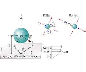
We consider the quasi-steady motion of a microswimmer in a Newtonian fluid near a solid surface, along which the no-slip condition of fluid velocity is violated and hydrodynamic slippage takes place. The schematic description of the problem geometry is presented in figure 1(a). The spherical cell body of the model microswimmer has a radius $a$
and its centre is at a distance
$a$
and its centre is at a distance $\tilde{h}$
from the adjacent slippery wall. The size of the microswimmer is small enough to neglect the inertial effects and at the same time not small enough that Brownian effects become dominant. The swimmer thrust is along
$\tilde{h}$
from the adjacent slippery wall. The size of the microswimmer is small enough to neglect the inertial effects and at the same time not small enough that Brownian effects become dominant. The swimmer thrust is along $\boldsymbol{e}$
, which is at a pitching angle
$\boldsymbol{e}$
, which is at a pitching angle $\unicode[STIX]{x1D703}$
relative to the wall. The azimuthal angle
$\unicode[STIX]{x1D703}$
relative to the wall. The azimuthal angle $\unicode[STIX]{x1D719}$
is the angle made by the horizontal projection of
$\unicode[STIX]{x1D719}$
is the angle made by the horizontal projection of $\boldsymbol{e}$
with the
$\boldsymbol{e}$
with the $x$
axis. Thus the director vector can be expressed in the fixed frame as follows:
$x$
axis. Thus the director vector can be expressed in the fixed frame as follows: $\boldsymbol{e}=\cos (\unicode[STIX]{x1D703})\cos (\unicode[STIX]{x1D719})\,\boldsymbol{i}_{x}+\cos (\unicode[STIX]{x1D703})\sin (\unicode[STIX]{x1D719})\,\boldsymbol{i}_{y}-\sin (\unicode[STIX]{x1D703})\,\boldsymbol{i}_{z}$
. However, in the presence of only axisymmetric squirming velocity at the microswimmer surface, we have
$\boldsymbol{e}=\cos (\unicode[STIX]{x1D703})\cos (\unicode[STIX]{x1D719})\,\boldsymbol{i}_{x}+\cos (\unicode[STIX]{x1D703})\sin (\unicode[STIX]{x1D719})\,\boldsymbol{i}_{y}-\sin (\unicode[STIX]{x1D703})\,\boldsymbol{i}_{z}$
. However, in the presence of only axisymmetric squirming velocity at the microswimmer surface, we have $\unicode[STIX]{x1D719}=0$
throughout the problem. The clockwise rotation along the
$\unicode[STIX]{x1D719}=0$
throughout the problem. The clockwise rotation along the $y$
axis is taken as positive. Here
$y$
axis is taken as positive. Here $\tilde{l}_{S}$
is the slip length denoting the extrapolation distance below the surface where the tangential fluid velocity would vanish. Here we assume that the fluid slippage is uniform over the plane wall and the effect of surface texture does not affect the microswimming characteristics.
$\tilde{l}_{S}$
is the slip length denoting the extrapolation distance below the surface where the tangential fluid velocity would vanish. Here we assume that the fluid slippage is uniform over the plane wall and the effect of surface texture does not affect the microswimming characteristics.
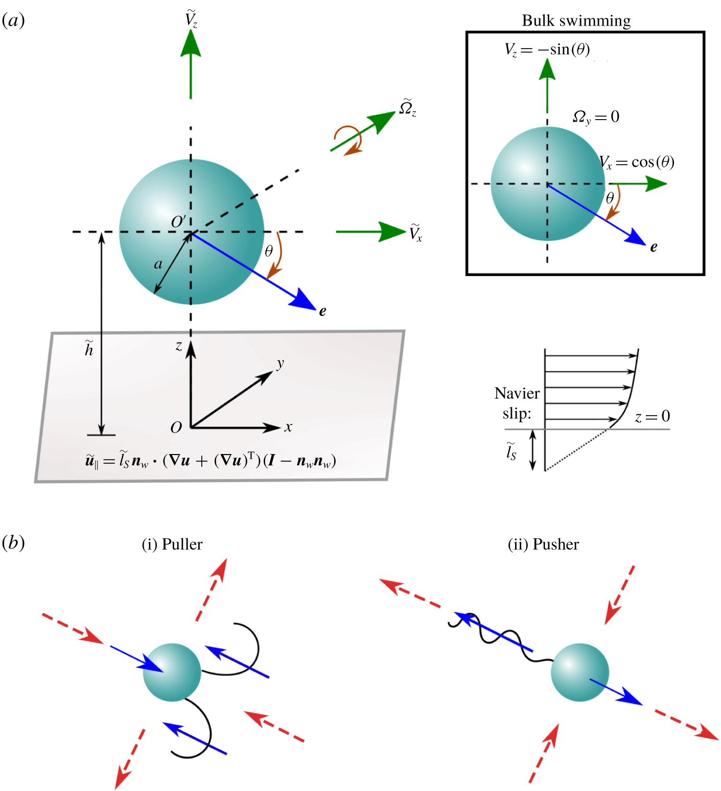
Figure 1. Schematic representation of a model microswimmer near a slippery flat surface obeying the Navier slip condition. (a) The microswimmer has a spherical cell body with radius $a$
. The direction of swimmer thrust or the director vector is indicated by
$a$
. The direction of swimmer thrust or the director vector is indicated by $\boldsymbol{e}$
. The angle
$\boldsymbol{e}$
. The angle $\unicode[STIX]{x1D703}$
is the pitching angle of the director relative to the wall. The adjacent flat surface has a slip length of
$\unicode[STIX]{x1D703}$
is the pitching angle of the director relative to the wall. The adjacent flat surface has a slip length of $\tilde{l}_{S}$
. The inset describes the corresponding situation when the microswimmer is far from the wall. The dimensionless swimming velocity components are also highlighted. (b) Puller and pusher swimmers having two different propulsion mechanisms are schematically shown in an unbounded domain. Red dashed arrows show surrounding fluid flow, while blue arrows indicate local forcing directions of the microswimmer to the fluid when viewed from the laboratory frame.
$\tilde{l}_{S}$
. The inset describes the corresponding situation when the microswimmer is far from the wall. The dimensionless swimming velocity components are also highlighted. (b) Puller and pusher swimmers having two different propulsion mechanisms are schematically shown in an unbounded domain. Red dashed arrows show surrounding fluid flow, while blue arrows indicate local forcing directions of the microswimmer to the fluid when viewed from the laboratory frame.
Neglecting the inertial effects, the flow field around the swimmer can be described by the incompressibility condition and Stokes equation as
 $$\begin{eqnarray}\unicode[STIX]{x1D735}\boldsymbol{\cdot }\tilde{\boldsymbol{v}}=0\quad \text{and}\quad -\unicode[STIX]{x1D735}\tilde{p}+\unicode[STIX]{x1D707}\unicode[STIX]{x1D6FB}^{2}\tilde{\boldsymbol{v}}=0.\end{eqnarray}$$
The hydrodynamic slippage at the confining wall is characterized by the Navier slip boundary condition (Navier Reference Navier1823), where the surface slip velocity has a linear variation with the shear rate at the plane surface, given as
 $$\begin{eqnarray}\tilde{\boldsymbol{u}}_{\Vert }=\tilde{l}_{S}\boldsymbol{n}_{w}\boldsymbol{\cdot }(\unicode[STIX]{x1D735}\boldsymbol{u}+(\unicode[STIX]{x1D735}\boldsymbol{u})^{\text{T}})(\unicode[STIX]{x1D644}-\boldsymbol{n}_{w}\boldsymbol{n}_{w}),\end{eqnarray}$$
where $\boldsymbol{n}_{w}$
is the unit normal at the plane wall pointing into the fluid and
$\boldsymbol{n}_{w}$
is the unit normal at the plane wall pointing into the fluid and $\boldsymbol{u}_{\Vert }$
is the velocity component tangential to the plane wall. The microswimmer gains motility from the surface distortions generated by their swimming appendages. Following the ‘squirmer’ model by Lighthill (Reference Lighthill1952) and Blake (Reference Blake1971), we impose a tangential velocity on a particle surface, which mimics the locomotion of microbes due to ciliary beating on their surface. The tangential surface velocity of a squirmer has the form
$\boldsymbol{u}_{\Vert }$
is the velocity component tangential to the plane wall. The microswimmer gains motility from the surface distortions generated by their swimming appendages. Following the ‘squirmer’ model by Lighthill (Reference Lighthill1952) and Blake (Reference Blake1971), we impose a tangential velocity on a particle surface, which mimics the locomotion of microbes due to ciliary beating on their surface. The tangential surface velocity of a squirmer has the form
 $$\begin{eqnarray}\tilde{\boldsymbol{u}}^{s}=\left(\frac{\boldsymbol{e}\boldsymbol{\cdot }\boldsymbol{r}}{|\boldsymbol{r}|}\frac{\boldsymbol{r}}{|\boldsymbol{r}|}-\boldsymbol{e}\right)\mathop{\sum }_{n=1}^{\infty }\frac{2}{n(n+1)}B_{n}P_{n}^{\prime }\left(\frac{\boldsymbol{e}\boldsymbol{\cdot }\boldsymbol{r}}{|\boldsymbol{r}|}\right),\end{eqnarray}$$
where $\boldsymbol{e}$
is the orientation vector of the director of the swimmer,
$\boldsymbol{e}$
is the orientation vector of the director of the swimmer, $\boldsymbol{r}$
is the position vector of an arbitrary point on the swimmer surface with respect to the particle centre,
$\boldsymbol{r}$
is the position vector of an arbitrary point on the swimmer surface with respect to the particle centre, $B_{n}$
denotes the
$B_{n}$
denotes the $n$
th squirming mode amplitude and
$n$
th squirming mode amplitude and $P_{n}^{\prime }$
is the derivative of the Legendre polynomial,
$P_{n}^{\prime }$
is the derivative of the Legendre polynomial, $P_{n}$
. The tangential velocity is assumed to be time-independent and represents an average over numerous beating cycles.
$P_{n}$
. The tangential velocity is assumed to be time-independent and represents an average over numerous beating cycles.
Following earlier studies (Ishikawa et al.
Reference Ishikawa, Simmonds and Pedley2006; Li & Ardekani Reference Li and Ardekani2014; Shaik & Ardekani Reference Shaik and Ardekani2017; Yazdi & Borhan Reference Yazdi and Borhan2017; Shen, Würger & Lintuvuori Reference Shen, Würger and Lintuvuori2018), we consider only the first two squirming modes. Depending on the ratio of the first two squirming mode amplitudes, we define a squirmer parameter, $\unicode[STIX]{x1D6FD}=B_{2}/B_{1}$
, which characterizes the intensity of the stresslet exerted by the swimmer. Pusher-type swimmers, e.g. bacteria or sperm cells, which have the flagella behind the main cell body, correspond to
$\unicode[STIX]{x1D6FD}=B_{2}/B_{1}$
, which characterizes the intensity of the stresslet exerted by the swimmer. Pusher-type swimmers, e.g. bacteria or sperm cells, which have the flagella behind the main cell body, correspond to $\unicode[STIX]{x1D6FD}>0$
; while, in contrast, pullers have their flagella in the front, e.g. Chlamydomonas. The distinct propulsion mechanisms of these swimmers are shown schematically in figure 1(b). Also,
$\unicode[STIX]{x1D6FD}>0$
; while, in contrast, pullers have their flagella in the front, e.g. Chlamydomonas. The distinct propulsion mechanisms of these swimmers are shown schematically in figure 1(b). Also, $\unicode[STIX]{x1D6FD}=0$
denotes the class of swimmers generating a symmetric flow field and which are designated as neutral swimmers, e.g. Volvox. We non-dimensionalize the lengths by the swimmer radius
$\unicode[STIX]{x1D6FD}=0$
denotes the class of swimmers generating a symmetric flow field and which are designated as neutral swimmers, e.g. Volvox. We non-dimensionalize the lengths by the swimmer radius $a$
, velocity by
$a$
, velocity by $U_{ref}=2B_{1}/3$
(so that the unbounded-medium squirming velocity becomes unity as shown in the inset of figure 1
a), time by
$U_{ref}=2B_{1}/3$
(so that the unbounded-medium squirming velocity becomes unity as shown in the inset of figure 1
a), time by $a/U_{ref}$
and pressure by
$a/U_{ref}$
and pressure by $\unicode[STIX]{x1D707}U_{ref}/a$
. Hereafter, the normalized variables will be denoted without the
$\unicode[STIX]{x1D707}U_{ref}/a$
. Hereafter, the normalized variables will be denoted without the $\,\tilde{~}\,$
symbol.
$\,\tilde{~}\,$
symbol.
If the microswimmer has a translational velocity of $\boldsymbol{V}$
and a rotational velocity of
$\boldsymbol{V}$
and a rotational velocity of $\unicode[STIX]{x1D734}$
, then, in the laboratory frame, the boundary condition for the fluid velocity at the surface of the swimmer can be written as
$\unicode[STIX]{x1D734}$
, then, in the laboratory frame, the boundary condition for the fluid velocity at the surface of the swimmer can be written as
 $$\begin{eqnarray}\boldsymbol{u}_{s}=\boldsymbol{V}+\unicode[STIX]{x1D734}\times \boldsymbol{r}+\boldsymbol{u}^{s}.\end{eqnarray}$$
In addition, since the swimmer is assumed to be neutrally buoyant in the suspending fluid, it experiences zero net force and zero net torque about its centre, i.e.
 $$\begin{eqnarray}\boldsymbol{F}=\iint _{S_{p}}\unicode[STIX]{x1D748}\boldsymbol{\cdot }\boldsymbol{n}_{p}\,\text{d}S=0\quad \text{and}\quad \boldsymbol{L}=\iint _{S_{p}}\boldsymbol{r}\times (\unicode[STIX]{x1D748}\boldsymbol{\cdot }\boldsymbol{n}_{p})\,\text{d}S=0,\end{eqnarray}$$
where $\unicode[STIX]{x1D748}$
is the stress tensor and
$\unicode[STIX]{x1D748}$
is the stress tensor and $\boldsymbol{n}_{p}$
is the unit outward normal to the swimmer surface
$\boldsymbol{n}_{p}$
is the unit outward normal to the swimmer surface $S_{p}$
. Now, solving (2.1) along with the boundary conditions (2.2) and (2.4), one can obtain
$S_{p}$
. Now, solving (2.1) along with the boundary conditions (2.2) and (2.4), one can obtain $\boldsymbol{V}$
and
$\boldsymbol{V}$
and $\unicode[STIX]{x1D734}$
by satisfying (2.5).
$\unicode[STIX]{x1D734}$
by satisfying (2.5).
Owing to the axisymmetric squirmer surface velocity in the present model (2.3), the director $\boldsymbol{e}$
of the swimmer is confined in the
$\boldsymbol{e}$
of the swimmer is confined in the $x{-}z$
plane. Also, it will rotate around an axis directed along
$x{-}z$
plane. Also, it will rotate around an axis directed along $\boldsymbol{n}_{w}\times \boldsymbol{e}$
. For the chosen coordinate system, this lies along the
$\boldsymbol{n}_{w}\times \boldsymbol{e}$
. For the chosen coordinate system, this lies along the $y$
axis. Hence, the locomotion of the microswimmer can be described by
$y$
axis. Hence, the locomotion of the microswimmer can be described by $\{\boldsymbol{V},\unicode[STIX]{x1D734}\}=\{V_{x}\boldsymbol{i}_{x}+V_{z}\boldsymbol{i}_{z},\unicode[STIX]{x1D6FA}_{y}\boldsymbol{i}_{y}\}$
.
$\{\boldsymbol{V},\unicode[STIX]{x1D734}\}=\{V_{x}\boldsymbol{i}_{x}+V_{z}\boldsymbol{i}_{z},\unicode[STIX]{x1D6FA}_{y}\boldsymbol{i}_{y}\}$
.
2.2 Exact solution using bispherical coordinates
The Stokes equation, coupled with the pertinent boundary conditions, including interfacial slip, is solved in terms of the eigensolutions for bispherical coordinates $(\unicode[STIX]{x1D709},\unicode[STIX]{x1D702},\unicode[STIX]{x1D719})$
. The velocity components are evaluated in a cylindrical coordinate system
$(\unicode[STIX]{x1D709},\unicode[STIX]{x1D702},\unicode[STIX]{x1D719})$
. The velocity components are evaluated in a cylindrical coordinate system $(\unicode[STIX]{x1D70C},z,\unicode[STIX]{x1D719})$
having its origin at the plane wall, the
$(\unicode[STIX]{x1D70C},z,\unicode[STIX]{x1D719})$
having its origin at the plane wall, the $z$
axis being normal to the wall and passing through the centre of the spherical swimmer body. The bispherical and cylindrical coordinates are related as (Happel & Brenner Reference Happel and Brenner1981)
$z$
axis being normal to the wall and passing through the centre of the spherical swimmer body. The bispherical and cylindrical coordinates are related as (Happel & Brenner Reference Happel and Brenner1981)
 $$\begin{eqnarray}\unicode[STIX]{x1D70C}=c\frac{\sin (\unicode[STIX]{x1D702})}{\cosh (\unicode[STIX]{x1D709})-\cos (\unicode[STIX]{x1D702})}\quad \text{and}\quad z=c\frac{\sinh (\unicode[STIX]{x1D709})}{\cosh (\unicode[STIX]{x1D709})-\cos (\unicode[STIX]{x1D702})},\end{eqnarray}$$
where $c$
is a positive scale factor. Here
$c$
is a positive scale factor. Here $\unicode[STIX]{x1D709}=0$
represents the plane wall and
$\unicode[STIX]{x1D709}=0$
represents the plane wall and $\unicode[STIX]{x1D709}=\unicode[STIX]{x1D709}_{0}$
(where
$\unicode[STIX]{x1D709}=\unicode[STIX]{x1D709}_{0}$
(where $\unicode[STIX]{x1D709}_{0}>0$
) denotes the surface of the sphere, which has its centre at
$\unicode[STIX]{x1D709}_{0}>0$
) denotes the surface of the sphere, which has its centre at $z=c\coth (\unicode[STIX]{x1D709}_{0})$
and has a radius of
$z=c\coth (\unicode[STIX]{x1D709}_{0})$
and has a radius of $c/\sinh (\unicode[STIX]{x1D709}_{0})$
. A schematic diagram describing the relation between the bispherical and a related cylindrical system has been provided in appendix A.
$c/\sinh (\unicode[STIX]{x1D709}_{0})$
. A schematic diagram describing the relation between the bispherical and a related cylindrical system has been provided in appendix A.
The general solution of the flow field was given by Lee & Leal (Reference Lee and Leal1980) with the help of seven unknown constants ( $A_{n}^{m},B_{n}^{m},C_{n}^{m},E_{n}^{m},F_{n}^{m},G_{n}^{m},H_{m}^{n}$
) and associated Legendre polynomial,
$A_{n}^{m},B_{n}^{m},C_{n}^{m},E_{n}^{m},F_{n}^{m},G_{n}^{m},H_{m}^{n}$
) and associated Legendre polynomial, $P_{n}^{m}=P_{n}^{m}(\cos (\unicode[STIX]{x1D702}))$
. Using the same general solution, researchers have solved the flow fields due to squirming microswimmer problems near a two-fluid interface (Shaik & Ardekani Reference Shaik and Ardekani2017; Yazdi & Borhan Reference Yazdi and Borhan2017) or the problem of a diffusiophoretic swimmer near a no-slip plane wall (Mozaffari et al.
Reference Mozaffari, Sharifi-Mood, Koplik and Maldarelli2016). In sharp contrast, here, the situation is more complex, since both the squirmer boundary condition at the swimmer surface, equation (2.4), as well as the Navier slip condition at the plane wall, equation (2.2), are to be satisfied while obtaining the arbitrary constants. In the cylindrical coordinates, the slip boundary condition at the plane wall reads
$P_{n}^{m}=P_{n}^{m}(\cos (\unicode[STIX]{x1D702}))$
. Using the same general solution, researchers have solved the flow fields due to squirming microswimmer problems near a two-fluid interface (Shaik & Ardekani Reference Shaik and Ardekani2017; Yazdi & Borhan Reference Yazdi and Borhan2017) or the problem of a diffusiophoretic swimmer near a no-slip plane wall (Mozaffari et al.
Reference Mozaffari, Sharifi-Mood, Koplik and Maldarelli2016). In sharp contrast, here, the situation is more complex, since both the squirmer boundary condition at the swimmer surface, equation (2.4), as well as the Navier slip condition at the plane wall, equation (2.2), are to be satisfied while obtaining the arbitrary constants. In the cylindrical coordinates, the slip boundary condition at the plane wall reads
 $$\begin{eqnarray}u_{\unicode[STIX]{x1D70C}}=l_{S}\unicode[STIX]{x1D70E}_{\unicode[STIX]{x1D70C}z}\quad \text{and}\quad u_{\unicode[STIX]{x1D719}}=l_{S}\unicode[STIX]{x1D70E}_{\unicode[STIX]{x1D719}z}\quad \text{at }z=0.\end{eqnarray}$$
Using the no-penetration condition of fluid at this surface, the above equations get simplified to
 $$\begin{eqnarray}u_{\unicode[STIX]{x1D70C}}=l_{S}\frac{\unicode[STIX]{x2202}u_{\unicode[STIX]{x1D70C}}}{\unicode[STIX]{x2202}z}\quad \text{and}\quad u_{\unicode[STIX]{x1D719}}=l_{S}\frac{\unicode[STIX]{x2202}u_{\unicode[STIX]{x1D719}}}{\unicode[STIX]{x2202}z}\quad \text{at }z=0.\end{eqnarray}$$
It is noteworthy to observe that, although acting in a regime of low-Reynolds-number flow, the wall slip effects are not obtained as a trivial extension to previously researched studies on a microswimmer near a no-slip wall. Also, the present approach differs from the asymptotic perturbation approach in terms of a small slip length as a perturbation parameter, which has been employed previously for unbounded particles with inhomogeneous surface slip (Swan & Khair Reference Swan and Khair2008; Willmott Reference Willmott2008; Ramachandran & Khair Reference Ramachandran and Khair2009). In effect, our results demonstrate that the effects of the fluid slip at the wall, manifested through the dimensionless slip length $l_{S}$
, modify the velocity field in a rather intriguing and non-trivial manner. Further details regarding the solution procedure have been provided in appendix B. The exact solution approach deployed by us, using bispherical coordinates, can incorporate any separation distance from the wall and any degree of wall slip (Lee & Leal Reference Lee and Leal1980; Kezirian Reference Kezirian1992; Loussaief, Pasol & Feuillebois Reference Loussaief, Pasol and Feuillebois2015). Thus it stands as a unified approach that circumvents the necessity of two different analysis tools in different regimes, i.e. an image-singularity-based far-field analysis (Spagnolie & Lauga Reference Spagnolie and Lauga2012; Lopez & Lauga Reference Lopez and Lauga2014) and a singular perturbation analysis in the lubrication regime (Ishikawa et al.
Reference Ishikawa, Simmonds and Pedley2006).
$l_{S}$
, modify the velocity field in a rather intriguing and non-trivial manner. Further details regarding the solution procedure have been provided in appendix B. The exact solution approach deployed by us, using bispherical coordinates, can incorporate any separation distance from the wall and any degree of wall slip (Lee & Leal Reference Lee and Leal1980; Kezirian Reference Kezirian1992; Loussaief, Pasol & Feuillebois Reference Loussaief, Pasol and Feuillebois2015). Thus it stands as a unified approach that circumvents the necessity of two different analysis tools in different regimes, i.e. an image-singularity-based far-field analysis (Spagnolie & Lauga Reference Spagnolie and Lauga2012; Lopez & Lauga Reference Lopez and Lauga2014) and a singular perturbation analysis in the lubrication regime (Ishikawa et al.
Reference Ishikawa, Simmonds and Pedley2006).
The complete swimming problem is decomposed into a thrust problem (considering the case when the swimmer is held fixed and experiencing only a tangential surface velocity) and a drag problem (when it undergoes a rigid-body motion with $\{\boldsymbol{V},\unicode[STIX]{x1D734}\}$
and experiences hydrodynamic drag). In the
$\{\boldsymbol{V},\unicode[STIX]{x1D734}\}$
and experiences hydrodynamic drag). In the $z$
direction, the force-free condition (2.5) reduces to
$z$
direction, the force-free condition (2.5) reduces to
 $$\begin{eqnarray}\displaystyle & \displaystyle F_{z,T}^{(Drag)}+F_{z}^{(Thrust)}=0, & \displaystyle\end{eqnarray}$$
 $$\begin{eqnarray}\displaystyle & \displaystyle F_{x,T}^{(Drag)}+F_{x,R}^{(Drag)}+F_{x}^{(Thrust)}=0, & \displaystyle\end{eqnarray}$$
 $$\begin{eqnarray}\displaystyle & \displaystyle L_{y,T}^{(Drag)}+L_{y,R}^{(Drag)}+L_{y}^{(Thrust)}=0. & \displaystyle\end{eqnarray}$$ $f$
’) as
$f$
’) as $F_{z,T}^{(Drag)}=f_{z,T}V_{z}$
,
$F_{z,T}^{(Drag)}=f_{z,T}V_{z}$
, $F_{x,T}^{(Drag)}=f_{x,T}V_{x}$
,
$F_{x,T}^{(Drag)}=f_{x,T}V_{x}$
, $F_{x,R}^{(Drag)}=f_{x,R}\unicode[STIX]{x1D6FA}_{y}$
,
$F_{x,R}^{(Drag)}=f_{x,R}\unicode[STIX]{x1D6FA}_{y}$
, $L_{y,T}^{(Drag)}=f_{y,T}V_{x}$
and
$L_{y,T}^{(Drag)}=f_{y,T}V_{x}$
and $L_{y,R}^{(Drag)}=f_{y,R}\unicode[STIX]{x1D6FA}_{y}$
. In these expressions, the first subscript represents the direction of the force or torque while the second subscript tells whether a particular drag force or torque is developed due to translation without rotation
$L_{y,R}^{(Drag)}=f_{y,R}\unicode[STIX]{x1D6FA}_{y}$
. In these expressions, the first subscript represents the direction of the force or torque while the second subscript tells whether a particular drag force or torque is developed due to translation without rotation $(T)$
or rotation without translation
$(T)$
or rotation without translation $(R)$
. The hydrodynamic resistance coefficients are functions of only the distance of the microswimmer from the wall
$(R)$
. The hydrodynamic resistance coefficients are functions of only the distance of the microswimmer from the wall $(h)$
and the slip length
$(h)$
and the slip length $(l_{S})$
, while the thrust force and torque are also dependent on the squirmer variables
$(l_{S})$
, while the thrust force and torque are also dependent on the squirmer variables $\unicode[STIX]{x1D6FD}$
and
$\unicode[STIX]{x1D6FD}$
and $\unicode[STIX]{x1D703}$
. Once the solution of a particular ‘fundamental problem’ (see appendix C for details) is found, the resistance coefficients, the thrust force and the torque can be determined by series summations in terms of the constants in the eigenfunction expansions (see (C 1)–(C 8) for details). Hence, the velocity components
$\unicode[STIX]{x1D703}$
. Once the solution of a particular ‘fundamental problem’ (see appendix C for details) is found, the resistance coefficients, the thrust force and the torque can be determined by series summations in terms of the constants in the eigenfunction expansions (see (C 1)–(C 8) for details). Hence, the velocity components $V_{x}$
,
$V_{x}$
, $V_{z}$
and
$V_{z}$
and $\unicode[STIX]{x1D6FA}_{y}$
are easily obtained by solving (2.9a
)–(2.9c
).
$\unicode[STIX]{x1D6FA}_{y}$
are easily obtained by solving (2.9a
)–(2.9c
).
It is noteworthy that the propulsive force and torque on the microswimmer can be alternatively determined without solving the Stokes equation by utilizing the Reynolds reciprocal theorem. The details of this approach applicable for the present problem is provided in appendix D.
3 Results and discussions
Towards investigating the microswimmer trajectories, we solve the following dynamic system:
 $$\begin{eqnarray}\frac{\text{d}x(t)}{\text{d}t}=V_{x},\quad \frac{\text{d}h(t)}{\text{d}t}=V_{z},\quad \frac{\text{d}\unicode[STIX]{x1D703}(t)}{\text{d}t}=\unicode[STIX]{x1D6FA}_{y}.\end{eqnarray}$$
Here we do not consider any stochastic motion due to translational or rotational diffusion, and the trajectories are computed based on deterministic forces only. The close approach of a microswimmer towards the wall often leads to the swimmer crashing against the wall and the subsequent motion becomes untraceable. To overcome this problem, we employ an additional short-range repulsive force of the form (Spagnolie & Lauga Reference Spagnolie and Lauga2012) $\boldsymbol{F}_{rep}=[(\unicode[STIX]{x1D6FC}_{1}\exp (-\unicode[STIX]{x1D6FC}_{2}\unicode[STIX]{x1D6FF}))/(1-\exp (-\unicode[STIX]{x1D6FC}_{2}\unicode[STIX]{x1D6FF}))]\boldsymbol{i}_{z}$
. Following Spagnolie & Lauga (Reference Spagnolie and Lauga2012) the parameter values
$\boldsymbol{F}_{rep}=[(\unicode[STIX]{x1D6FC}_{1}\exp (-\unicode[STIX]{x1D6FC}_{2}\unicode[STIX]{x1D6FF}))/(1-\exp (-\unicode[STIX]{x1D6FC}_{2}\unicode[STIX]{x1D6FF}))]\boldsymbol{i}_{z}$
. Following Spagnolie & Lauga (Reference Spagnolie and Lauga2012) the parameter values $\unicode[STIX]{x1D6FC}_{1}=100$
and
$\unicode[STIX]{x1D6FC}_{1}=100$
and $\unicode[STIX]{x1D6FC}_{2}=100$
are chosen to prevent the swimmer coming closer than a distance of
$\unicode[STIX]{x1D6FC}_{2}=100$
are chosen to prevent the swimmer coming closer than a distance of ${\sim}0.01$
times the swimmer radius from the wall. Such forces originate from the nanoscale interaction between the swimmer body and the wall surface, especially in physiological conditions (Klein, Clapp & Dickinson Reference Klein, Clapp and Dickinson2003). Diverse forms of repulsive forces have been employed in the literature (Li & Ardekani Reference Li and Ardekani2014; Hu et al.
Reference Hu, Wysocki, Winkler and Gompper2015; Katuri et al.
Reference Katuri, Uspal, Simmchen, Miguel-López and Sánchez2018; Walker et al.
Reference Walker, Wheeler, Ishimoto and Gaffney2019). It is to be noted that the use of a short-range repulsive force at the wall destroys the puller–pusher duality during time reversal (Ishimoto Reference Ishimoto2017; Walker et al.
Reference Walker, Wheeler, Ishimoto and Gaffney2019).
${\sim}0.01$
times the swimmer radius from the wall. Such forces originate from the nanoscale interaction between the swimmer body and the wall surface, especially in physiological conditions (Klein, Clapp & Dickinson Reference Klein, Clapp and Dickinson2003). Diverse forms of repulsive forces have been employed in the literature (Li & Ardekani Reference Li and Ardekani2014; Hu et al.
Reference Hu, Wysocki, Winkler and Gompper2015; Katuri et al.
Reference Katuri, Uspal, Simmchen, Miguel-López and Sánchez2018; Walker et al.
Reference Walker, Wheeler, Ishimoto and Gaffney2019). It is to be noted that the use of a short-range repulsive force at the wall destroys the puller–pusher duality during time reversal (Ishimoto Reference Ishimoto2017; Walker et al.
Reference Walker, Wheeler, Ishimoto and Gaffney2019).
First we illustrate the wall-slip-mediated alterations in the translational and rotational velocity components of different types of squirmers having a spherical cell body. Subsequently, the resulting trajectories are elucidated and different phase transitions of swimming states are discussed. Considering a typical microswimmer radius in the range of $1{-}100~\unicode[STIX]{x03BC}\text{m}$
and in view of the experimentally observed dimensional slip lengths (Zhu & Granick Reference Zhu and Granick2001; Tretheway & Meinhart Reference Tretheway and Meinhart2002; Huang et al.
Reference Huang, Sendner, Horinek, Netz and Bocquet2008), we take the dimensionless slip length
$1{-}100~\unicode[STIX]{x03BC}\text{m}$
and in view of the experimentally observed dimensional slip lengths (Zhu & Granick Reference Zhu and Granick2001; Tretheway & Meinhart Reference Tretheway and Meinhart2002; Huang et al.
Reference Huang, Sendner, Horinek, Netz and Bocquet2008), we take the dimensionless slip length $(l_{S})$
in the range of 0 to 10.
$(l_{S})$
in the range of 0 to 10.
3.1 Swimming velocity alterations
Figure 2 portrays the effects of slip length $(l_{S})$
on the velocity components
$(l_{S})$
on the velocity components $(V_{z},V_{x},\unicode[STIX]{x1D6FA}_{y})$
at different separation distances of the microswimmer from the wall
$(V_{z},V_{x},\unicode[STIX]{x1D6FA}_{y})$
at different separation distances of the microswimmer from the wall $(\unicode[STIX]{x1D6FF})$
. In many situations the said effects turn out to be different in nature, if not opposite, for the puller- and pusher-type microswimmers. To understand the physical origin of the same, we first look into the fundamental differences in the propulsion mechanisms and surrounding flow patterns associated with these two types of swimmers in an unbounded domain.
$(\unicode[STIX]{x1D6FF})$
. In many situations the said effects turn out to be different in nature, if not opposite, for the puller- and pusher-type microswimmers. To understand the physical origin of the same, we first look into the fundamental differences in the propulsion mechanisms and surrounding flow patterns associated with these two types of swimmers in an unbounded domain.
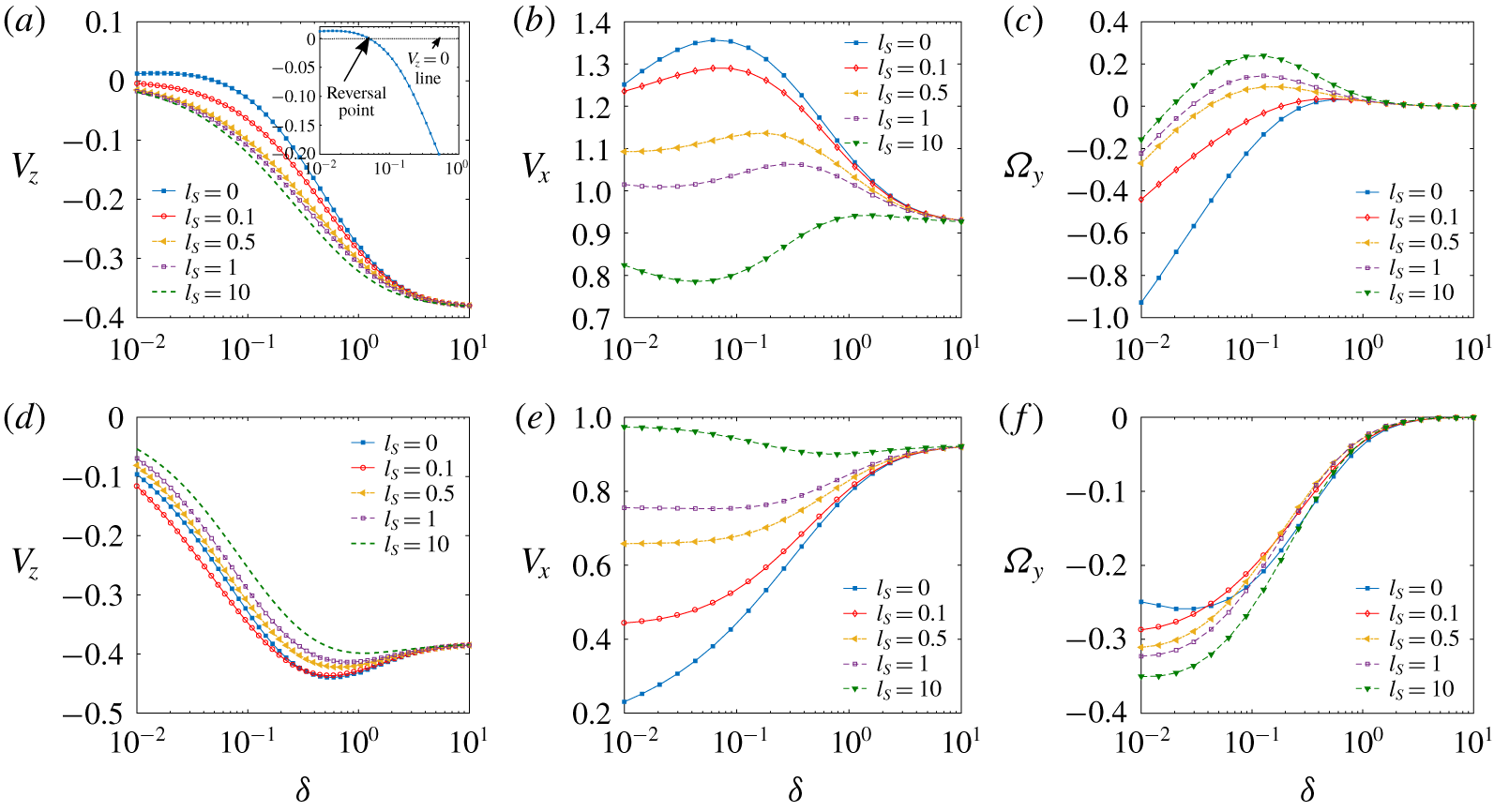
Figure 2. Velocity components of a microswimmer versus smallest separation distance from the wall $(\unicode[STIX]{x1D6FF}=h-1)$
for different slip lengths
$(\unicode[STIX]{x1D6FF}=h-1)$
for different slip lengths $(l_{S})$
. Panels (a–c) are for a puller and (d–f) are for a pusher, all having a squirmer parameter value
$(l_{S})$
. Panels (a–c) are for a puller and (d–f) are for a pusher, all having a squirmer parameter value $|\unicode[STIX]{x1D6FD}|=4$
and angular orientation
$|\unicode[STIX]{x1D6FD}|=4$
and angular orientation $\unicode[STIX]{x1D703}=\unicode[STIX]{x03C0}/8$
. In the inset of (a), a magnified view of the no-slip case is shown.
$\unicode[STIX]{x1D703}=\unicode[STIX]{x03C0}/8$
. In the inset of (a), a magnified view of the no-slip case is shown.
Figure 3. Velocity field around both puller-type (a,c,e) and pusher-type (b,d,f) microswimmers in the $x$
–
$x$
– $z$
plane for pitching angle
$z$
plane for pitching angle $\unicode[STIX]{x1D703}=\unicode[STIX]{x03C0}/8$
and
$\unicode[STIX]{x1D703}=\unicode[STIX]{x03C0}/8$
and $|\unicode[STIX]{x1D6FD}|=4$
. The rows (from top to bottom) correspond to the situations of an unbounded microswimmer, a microswimmer near a no-slip surface and near a slippery surface
$|\unicode[STIX]{x1D6FD}|=4$
. The rows (from top to bottom) correspond to the situations of an unbounded microswimmer, a microswimmer near a no-slip surface and near a slippery surface $(l_{S}=5)$
, respectively. Distance from the wall is taken as
$(l_{S}=5)$
, respectively. Distance from the wall is taken as $\unicode[STIX]{x1D6FF}=0.2$
. The colour scale depicts the fluid velocity magnitude and the streamlines are shown in the laboratory frame.
$\unicode[STIX]{x1D6FF}=0.2$
. The colour scale depicts the fluid velocity magnitude and the streamlines are shown in the laboratory frame.
Pullers have their flagella ahead of their cell body and the thrust generated by the flagella is cancelled by the cell body at the back. Thus, at large length scales, a moving puller squirmer gives rise to a contractile dipolar flow in the surroundings (figure 1
bi). In contrast, pushers have their flagella at the back and the thrust is generated from behind, thereby mimicking a extensile dipolar flow at large length scales (figure 1
bii). Also, beyond a sufficient stirring action created due to the second squirming mode $(|\unicode[STIX]{x1D6FD}|>1)$
, a pair of circulation rolls, symmetric about the direction of motion, is observed from a comoving frame, but at different locations, behind the cell body for a puller but ahead of the cell body for a pusher (Magar, Goto & Pedley Reference Magar, Goto and Pedley2003; De Corato, Greco & Maffettone Reference De Corato, Greco and Maffettone2015).
$(|\unicode[STIX]{x1D6FD}|>1)$
, a pair of circulation rolls, symmetric about the direction of motion, is observed from a comoving frame, but at different locations, behind the cell body for a puller but ahead of the cell body for a pusher (Magar, Goto & Pedley Reference Magar, Goto and Pedley2003; De Corato, Greco & Maffettone Reference De Corato, Greco and Maffettone2015).
The flow field around the squirmer and the wall can be visualized from figure 3. Considering the illustrated situation, when swimmers of both types are pointing towards the wall, the effect of wall-reflected flow is first sensed by their flagella in the case of a puller and the thrust created by their breaststroke action gets affected due to a confinement. In contrast, the frontal cell body of the pusher will be the first to experience the distorted flow, which must be adjusted by a modified pushing action by their posterior flagella. Evidently, the stress distribution around the swimmer will also face modifications based on the relative position of the cell body and the flagella and the corresponding flow adjustments created by them. The presence of wall slip further complicates the scenario by allowing a non-zero tangential fluid velocity at the plane wall. Consequently, the pattern and intensity of the micro-vortices around the squirmer get adjusted differently as demonstrated in figure 3(e,f). This not only creates alterations in the propulsive action of the swimmer and but also modifies the hydrodynamic resistance to a finite-size cell body moving near the wall.
In figure 2(a) the effect of wall slip on the wall-normal velocity component $V_{z}$
is shown for a puller microswimmer with locations ranging from very close to far away separations from the plane wall. The spherical cell body faces different extents of surface stresses due to a near-wall movement. The narrow gap between the swimmer body and the wall generates large velocity gradients, which result in enhanced surface stress in the lower half of the sphere in comparison to the upper half, which does not encounter the wall directly. Hocking (Reference Hocking1973) showed that the presence of wall slip results in a logarithmic increase in
$V_{z}$
is shown for a puller microswimmer with locations ranging from very close to far away separations from the plane wall. The spherical cell body faces different extents of surface stresses due to a near-wall movement. The narrow gap between the swimmer body and the wall generates large velocity gradients, which result in enhanced surface stress in the lower half of the sphere in comparison to the upper half, which does not encounter the wall directly. Hocking (Reference Hocking1973) showed that the presence of wall slip results in a logarithmic increase in $f_{z,T}$
with
$f_{z,T}$
with $\unicode[STIX]{x1D6FF}$
and it becomes inversely proportional to the slip length
$\unicode[STIX]{x1D6FF}$
and it becomes inversely proportional to the slip length $(l_{S})$
. While considering the behaviour of microswimmer velocity
$(l_{S})$
. While considering the behaviour of microswimmer velocity $V_{z}$
, we also have to examine the thrust force variations shown in figure 4. Figure 4(a) demonstrates that a puller-type microswimmer experiences a decreasing thrust force when the wall is slip-free and it becomes negative after the separation exceeds a certain value. This is responsible for velocity reversal in figure 2(a). With increasing slip length, this reversal in
$V_{z}$
, we also have to examine the thrust force variations shown in figure 4. Figure 4(a) demonstrates that a puller-type microswimmer experiences a decreasing thrust force when the wall is slip-free and it becomes negative after the separation exceeds a certain value. This is responsible for velocity reversal in figure 2(a). With increasing slip length, this reversal in $V_{z}$
ceases to occur and it indicates a wall-approaching trend of the microswimmer for all separation distances, consistent with the thrust force variations.
$V_{z}$
ceases to occur and it indicates a wall-approaching trend of the microswimmer for all separation distances, consistent with the thrust force variations.

Figure 4. Variation of thrust force and torque components $(F_{z}^{(Thrust)},F_{x}^{(Thrust)},L_{y}^{(Thrust)})$
with wall separation distance
$(F_{z}^{(Thrust)},F_{x}^{(Thrust)},L_{y}^{(Thrust)})$
with wall separation distance $(\unicode[STIX]{x1D6FF})$
for different slip lengths
$(\unicode[STIX]{x1D6FF})$
for different slip lengths $(l_{S})$
. The parameters correspond to those of figure 2.
$(l_{S})$
. The parameters correspond to those of figure 2.
Figure 2(d) depicts that, for a pusher-type swimmer, the variations in $V_{z}$
are non-monotonic in both
$V_{z}$
are non-monotonic in both $\unicode[STIX]{x1D6FF}$
and
$\unicode[STIX]{x1D6FF}$
and $l_{S}$
, although the thrust force is monotonic (figure 4
d). Observing figure 5 we find that at very low wall separations
$l_{S}$
, although the thrust force is monotonic (figure 4
d). Observing figure 5 we find that at very low wall separations $(0.01\lesssim \unicode[STIX]{x1D6FF}\lesssim 0.1)$
there exists an intermediate slip length
$(0.01\lesssim \unicode[STIX]{x1D6FF}\lesssim 0.1)$
there exists an intermediate slip length $l_{S}\sim 0.1$
for which the wall-bound velocity becomes maximum in magnitude. This again indicates a considerable importance of hydrodynamic drag force variations on the swimmer velocity. Notably, the above observations for a pusher are in sharp contrast to the characteristics of a force dipole pusher, which, in the far-field analysis, always tends to get attracted to the wall with increasing slip length (Lopez & Lauga Reference Lopez and Lauga2014). Such disagreement arises from the fact that, in a force dipole model, the contributions from the higher-order singularities arising from a finite-size cell body or the fore–aft asymmetry of the swimmer are not taken into account (Spagnolie & Lauga Reference Spagnolie and Lauga2012). In addition to these far-field effects, in the present case, the near-field hydrodynamic interaction also plays its role in modifying the swimmer velocity.
$l_{S}\sim 0.1$
for which the wall-bound velocity becomes maximum in magnitude. This again indicates a considerable importance of hydrodynamic drag force variations on the swimmer velocity. Notably, the above observations for a pusher are in sharp contrast to the characteristics of a force dipole pusher, which, in the far-field analysis, always tends to get attracted to the wall with increasing slip length (Lopez & Lauga Reference Lopez and Lauga2014). Such disagreement arises from the fact that, in a force dipole model, the contributions from the higher-order singularities arising from a finite-size cell body or the fore–aft asymmetry of the swimmer are not taken into account (Spagnolie & Lauga Reference Spagnolie and Lauga2012). In addition to these far-field effects, in the present case, the near-field hydrodynamic interaction also plays its role in modifying the swimmer velocity.

Figure 5. Variation of wall-normal velocity $V_{z}$
of a pusher swimmer
$V_{z}$
of a pusher swimmer $(\unicode[STIX]{x1D6FD}=-4)$
with slip length for various wall separation distances
$(\unicode[STIX]{x1D6FD}=-4)$
with slip length for various wall separation distances $(\unicode[STIX]{x1D6FF})$
. Here microswimmer orientation,
$(\unicode[STIX]{x1D6FF})$
. Here microswimmer orientation, $\unicode[STIX]{x1D703}=\unicode[STIX]{x03C0}/8$
.
$\unicode[STIX]{x1D703}=\unicode[STIX]{x03C0}/8$
.
Figure 2(b) shows that the wall-parallel velocity $(V_{x})$
remains higher than the unbounded-medium velocity, i.e.
$(V_{x})$
remains higher than the unbounded-medium velocity, i.e. $(V_{x}\rightarrow \cos (\unicode[STIX]{x1D703}))$
for all wall separations, until the slip length becomes high enough (e.g.
$(V_{x}\rightarrow \cos (\unicode[STIX]{x1D703}))$
for all wall separations, until the slip length becomes high enough (e.g. $l_{S}=10$
) to cause
$l_{S}=10$
) to cause $V_{x}$
to fall below the unbounded-medium velocity. A fall in swimming velocity with increasing
$V_{x}$
to fall below the unbounded-medium velocity. A fall in swimming velocity with increasing $l_{S}$
is in contrast to intuition, since a spherical particle translating parallel to the wall experiences lower hydrodynamic resistance in the presence of slip (Davis, Kezirian & Brenner Reference Davis, Kezirian and Brenner1994; Loussaief et al.
Reference Loussaief, Pasol and Feuillebois2015). To address this apparent anomaly, we consider the fact that the microswimmer velocity is dependent on a coupled effect of the hydrodynamic resistances to the simultaneous translational and rotational movement parallel to the wall as well as on the thrust generated due to the propulsive action. Both the propulsive thrust force
$l_{S}$
is in contrast to intuition, since a spherical particle translating parallel to the wall experiences lower hydrodynamic resistance in the presence of slip (Davis, Kezirian & Brenner Reference Davis, Kezirian and Brenner1994; Loussaief et al.
Reference Loussaief, Pasol and Feuillebois2015). To address this apparent anomaly, we consider the fact that the microswimmer velocity is dependent on a coupled effect of the hydrodynamic resistances to the simultaneous translational and rotational movement parallel to the wall as well as on the thrust generated due to the propulsive action. Both the propulsive thrust force $(F_{x}^{(Thrust)})$
and torque
$(F_{x}^{(Thrust)})$
and torque $(L_{y}^{(Thrust)})$
are affected by wall slip as shown in figures 4(b) and 4(c), respectively. It is observed that the increase in
$(L_{y}^{(Thrust)})$
are affected by wall slip as shown in figures 4(b) and 4(c), respectively. It is observed that the increase in $F_{x}^{(Thrust)}$
with reducing swimmer–wall distances in the no-slip case is now slowed down by the wall slip effect. In addition, the wall slip acts to reduce the propulsive torque away from the wall and even makes it act in the reverse direction for extremely high slip lengths, but only for an intermediate range of wall separations (see figure 4
c). A propulsive torque towards the wall also contributes in reducing
$F_{x}^{(Thrust)}$
with reducing swimmer–wall distances in the no-slip case is now slowed down by the wall slip effect. In addition, the wall slip acts to reduce the propulsive torque away from the wall and even makes it act in the reverse direction for extremely high slip lengths, but only for an intermediate range of wall separations (see figure 4
c). A propulsive torque towards the wall also contributes in reducing $V_{x}$
, which can be confirmed from the final expression of
$V_{x}$
, which can be confirmed from the final expression of $V_{x}$
in (3.2a
).
$V_{x}$
in (3.2a
).
The sign of the angular velocity of a microswimmer near a wall $(\unicode[STIX]{x1D6FA}_{y})$
is determined by two main opposing physical mechanisms arising from the propulsive action: the torque whose direction depends on the direction of the slip flow at the surface of the swimmer, and the torque that always acts towards the wall due to the wall-parallel forward movement. The force-free conditions in (2.9) provide the following final expressions of
$(\unicode[STIX]{x1D6FA}_{y})$
is determined by two main opposing physical mechanisms arising from the propulsive action: the torque whose direction depends on the direction of the slip flow at the surface of the swimmer, and the torque that always acts towards the wall due to the wall-parallel forward movement. The force-free conditions in (2.9) provide the following final expressions of $V_{x}$
and
$V_{x}$
and $\unicode[STIX]{x1D6FA}_{y}$
:
$\unicode[STIX]{x1D6FA}_{y}$
:
 $$\begin{eqnarray}V_{x}={\displaystyle \frac{F_{x}^{(Thrust)}f_{y,R}-L_{y}^{(Thrust)}f_{x,R}}{f_{x,R}\,f_{y,T}-f_{x,T}f_{y,R}}}\quad \text{and}\quad \unicode[STIX]{x1D6FA}_{y}={\displaystyle \frac{\overbrace{L_{y}^{(Thrust)}f_{x,T}}^{T_{1}}-\overbrace{F_{x}^{(Thrust)}f_{y,T}}^{T_{2}}}{\underbrace{f_{x,R}\,f_{y,T}-f_{x,T}f_{y,R}}_{T_{3}}}}.\end{eqnarray}$$
They suggest that the hydrodynamic resistance factors are intrinsically coupled with the thrust force and torque and take part in deciding the resultant rotation direction. The effect of wall slip on the various terms contributing to the rotation rate are shown in figure 6. This shows that increasing wall slip drastically alters $T_{1}$
and
$T_{1}$
and $T_{3}$
, while changes in
$T_{3}$
, while changes in $T_{2}$
are not significant. In effect, for a puller swimmer the wall slip exerts a strong opposing torque to the swimmer rotation away from the wall
$T_{2}$
are not significant. In effect, for a puller swimmer the wall slip exerts a strong opposing torque to the swimmer rotation away from the wall $(\unicode[STIX]{x1D6FA}_{y}<0)$
, which for high slip lengths causes it to rotate towards the wall
$(\unicode[STIX]{x1D6FA}_{y}<0)$
, which for high slip lengths causes it to rotate towards the wall $(\unicode[STIX]{x1D6FA}_{y}>0)$
, before reaching the bulk zero-rotation state (refer to the inset of figure 1
a) at a distance of nearly one radius away from the wall, as demonstrated in figure 2(c).
$(\unicode[STIX]{x1D6FA}_{y}>0)$
, before reaching the bulk zero-rotation state (refer to the inset of figure 1
a) at a distance of nearly one radius away from the wall, as demonstrated in figure 2(c).


Variation of the thrust force $(F_{x}^{(Thrust)})$
for a pusher (see figure 4
e) is highly complex and non-monotonic in nature. However, the corresponding wall-parallel velocity component
$(F_{x}^{(Thrust)})$
for a pusher (see figure 4
e) is highly complex and non-monotonic in nature. However, the corresponding wall-parallel velocity component $(V_{x})$
shows a trend of getting escalated with slip length (see figure 2
e), a phenomenon that is exactly opposite to that of a puller. The negative thrust torque on the microswimmer gets reduced by the wall slip for all separations (see figure 4
f). Again, this fixed trend is not followed by the rotation rate
$(V_{x})$
shows a trend of getting escalated with slip length (see figure 2
e), a phenomenon that is exactly opposite to that of a puller. The negative thrust torque on the microswimmer gets reduced by the wall slip for all separations (see figure 4
f). Again, this fixed trend is not followed by the rotation rate $\unicode[STIX]{x1D6FA}_{y}$
. Figure 2(f) demonstrates that, for a pusher swimmer located very close to the wall
$\unicode[STIX]{x1D6FA}_{y}$
. Figure 2(f) demonstrates that, for a pusher swimmer located very close to the wall $(\unicode[STIX]{x1D6FF}\lesssim 0.04)$
, the wall slip forces it to rotate away from the wall. However, beyond this distance, the slip-induced rotation gets either escalated or suppressed, depending on a subtle interplay between slip and wall separation. This is again in contradiction to the previously studied far-field behaviour of a force dipole swimmer (Lopez & Lauga Reference Lopez and Lauga2014), due to the similar reasons discussed for
$(\unicode[STIX]{x1D6FF}\lesssim 0.04)$
, the wall slip forces it to rotate away from the wall. However, beyond this distance, the slip-induced rotation gets either escalated or suppressed, depending on a subtle interplay between slip and wall separation. This is again in contradiction to the previously studied far-field behaviour of a force dipole swimmer (Lopez & Lauga Reference Lopez and Lauga2014), due to the similar reasons discussed for $V_{z}$
.
$V_{z}$
.
3.2 Modulations in near-wall swimming trajectories
3.2.1 Neutral squirmer
A neutral squirmer, which is characterized by $\unicode[STIX]{x1D6FD}=0$
, gives rise to a quadrupolar flow field around the swimmer in an unbounded domain and thus vorticity is absent in the velocity field (Zhu et al.
Reference Zhu, Do-Quang, Lauga and Brandt2011; Zhu, Lauga & Brandt Reference Zhu, Lauga and Brandt2012). In the absence of the wall slip, for an initial orientation away from the wall or even with a small tilt towards the wall, a neutral swimmer does not show any tendency to move towards the wall and escapes from the wall along a straight line with the final orientation angle reaching an asymptotic constant value
$\unicode[STIX]{x1D6FD}=0$
, gives rise to a quadrupolar flow field around the swimmer in an unbounded domain and thus vorticity is absent in the velocity field (Zhu et al.
Reference Zhu, Do-Quang, Lauga and Brandt2011; Zhu, Lauga & Brandt Reference Zhu, Lauga and Brandt2012). In the absence of the wall slip, for an initial orientation away from the wall or even with a small tilt towards the wall, a neutral swimmer does not show any tendency to move towards the wall and escapes from the wall along a straight line with the final orientation angle reaching an asymptotic constant value $(\unicode[STIX]{x1D703}_{f})$
. The scenario changes for moderate values of the initial orientation angles towards the wall. As it moves towards the wall, its director gradually points away from the wall due to a net anticlockwise torque arising from the near-field hydrodynamic effect, which subsequently forces the swimmer to attain a negative orientation angle
$(\unicode[STIX]{x1D703}_{f})$
. The scenario changes for moderate values of the initial orientation angles towards the wall. As it moves towards the wall, its director gradually points away from the wall due to a net anticlockwise torque arising from the near-field hydrodynamic effect, which subsequently forces the swimmer to attain a negative orientation angle $\unicode[STIX]{x1D703}_{0}<0$
. In effect, the normal velocity component becomes positive
$\unicode[STIX]{x1D703}_{0}<0$
. In effect, the normal velocity component becomes positive $(V_{z}>0)$
, leading to the escape of the swimmer away from wall. Beyond a critical initial orientation,
$(V_{z}>0)$
, leading to the escape of the swimmer away from wall. Beyond a critical initial orientation, $\unicode[STIX]{x1D703}_{0,cr}$
, the swimmer eventually collides with the wall, remains in the wall-adjacent region for some time, and finally escapes with a final orientation equal to its initial one,
$\unicode[STIX]{x1D703}_{0,cr}$
, the swimmer eventually collides with the wall, remains in the wall-adjacent region for some time, and finally escapes with a final orientation equal to its initial one, $\unicode[STIX]{x1D703}_{f}\approx \unicode[STIX]{x1D703}_{0}$
. When the swimmer has an initial height of
$\unicode[STIX]{x1D703}_{f}\approx \unicode[STIX]{x1D703}_{0}$
. When the swimmer has an initial height of $h_{0}=2$
, this critical angle for descending to a height below
$h_{0}=2$
, this critical angle for descending to a height below $h=1.05$
has been reported to be
$h=1.05$
has been reported to be ${\sim}0.4$
by Spagnolie & Lauga (Reference Spagnolie and Lauga2012). We show in figure 7(a) that the critical angle for the transition of a scattering trajectory to a colliding one (with a cutoff distance for collision as
${\sim}0.4$
by Spagnolie & Lauga (Reference Spagnolie and Lauga2012). We show in figure 7(a) that the critical angle for the transition of a scattering trajectory to a colliding one (with a cutoff distance for collision as $h=1.01$
) shows a drastic decrease from the no-slip case (
$h=1.01$
) shows a drastic decrease from the no-slip case ( $l_{S}=0$
,
$l_{S}=0$
, $\unicode[STIX]{x1D703}_{0,cr}=0.59$
) to
$\unicode[STIX]{x1D703}_{0,cr}=0.59$
) to $\unicode[STIX]{x1D703}_{0,cr}=0.38$
for
$\unicode[STIX]{x1D703}_{0,cr}=0.38$
for $l_{S}=1$
and finally reaches an asymptote of
$l_{S}=1$
and finally reaches an asymptote of $\unicode[STIX]{x1D703}_{0,cr}\rightarrow 0.36$
for higher values of the wall slip length.
$\unicode[STIX]{x1D703}_{0,cr}\rightarrow 0.36$
for higher values of the wall slip length.
Here we define the wall-bound detention time of a microswimmer $(T_{det})$
by the time interval during which the microswimmer remains below a distance of one-tenth of its diameter. For a typical microswimmer diameter of
$(T_{det})$
by the time interval during which the microswimmer remains below a distance of one-tenth of its diameter. For a typical microswimmer diameter of $10$
to
$10$
to $30~\unicode[STIX]{x03BC}\text{m}$
, this cutoff distance remains consistent with the experimental evidence of E. coli cells remaining at a distance of
$30~\unicode[STIX]{x03BC}\text{m}$
, this cutoff distance remains consistent with the experimental evidence of E. coli cells remaining at a distance of ${<}1{-}3~\unicode[STIX]{x03BC}\text{m}$
near a wall (Drescher et al.
Reference Drescher, Dunkel, Cisneros, Ganguly and Goldstein2011) for an extended time. Figure 7(b) shows that, although the escaping nature of the microswimmer motion is preserved even with a very high slip length, the detention time for a neutral swimmer gets increased significantly with the slip length
${<}1{-}3~\unicode[STIX]{x03BC}\text{m}$
near a wall (Drescher et al.
Reference Drescher, Dunkel, Cisneros, Ganguly and Goldstein2011) for an extended time. Figure 7(b) shows that, although the escaping nature of the microswimmer motion is preserved even with a very high slip length, the detention time for a neutral swimmer gets increased significantly with the slip length $(l_{S})$
(see the inset of figure 7
b). Interestingly, for small tilt angles towards the wall (e.g.
$(l_{S})$
(see the inset of figure 7
b). Interestingly, for small tilt angles towards the wall (e.g. $\unicode[STIX]{x1D703}_{0}=0.05\unicode[STIX]{x03C0}$
), where the detention time is negligible near a no-slip wall, the increasing slip length beyond a critical value is found to impart a high detention time.
$\unicode[STIX]{x1D703}_{0}=0.05\unicode[STIX]{x03C0}$
), where the detention time is negligible near a no-slip wall, the increasing slip length beyond a critical value is found to impart a high detention time.
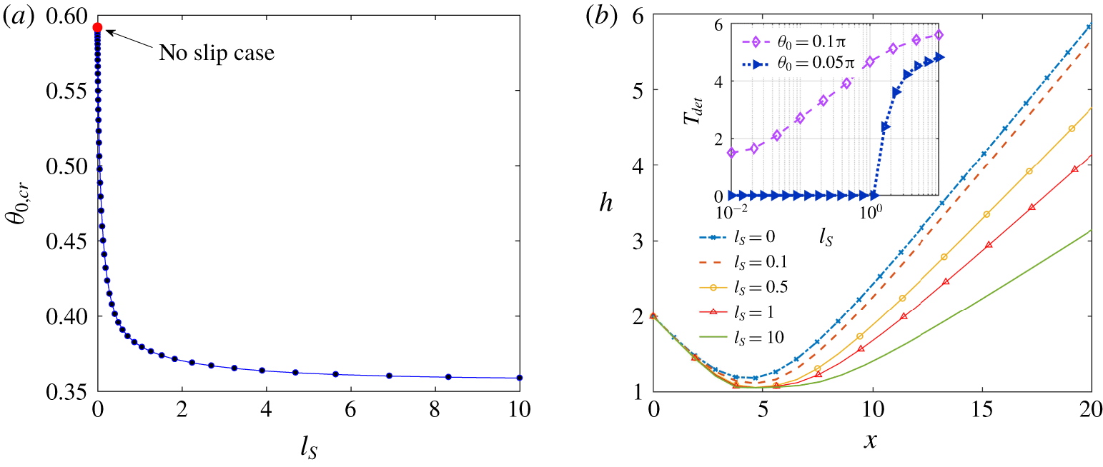
Figure 7. (a) Critical initial orientation $(\unicode[STIX]{x1D703}_{0,cr})$
versus slip length
$(\unicode[STIX]{x1D703}_{0,cr})$
versus slip length $(l_{S})$
. (b) Trajectory with initial orientation,
$(l_{S})$
. (b) Trajectory with initial orientation, $\unicode[STIX]{x1D703}_{0}=0.1\unicode[STIX]{x03C0}$
. In the inset the variation of dimensionless detention time with slip length is shown. In both panels the initial height,
$\unicode[STIX]{x1D703}_{0}=0.1\unicode[STIX]{x03C0}$
. In the inset the variation of dimensionless detention time with slip length is shown. In both panels the initial height, $h_{0}=2$
is taken.
$h_{0}=2$
is taken.
3.2.2 Puller squirmer
While swimming near a no-slip wall, the director $(\boldsymbol{e})$
does not face a hydrodynamic rotation relative to the wall if the strength of the vorticity generation term
$(\boldsymbol{e})$
does not face a hydrodynamic rotation relative to the wall if the strength of the vorticity generation term $(\propto \unicode[STIX]{x1D6FD})$
in the squirmer surface velocity is not sufficiently high (Ishimoto & Gaffney Reference Ishimoto and Gaffney2013). As
$(\propto \unicode[STIX]{x1D6FD})$
in the squirmer surface velocity is not sufficiently high (Ishimoto & Gaffney Reference Ishimoto and Gaffney2013). As $\unicode[STIX]{x1D6FD}$
crosses a critical value, the hydrodynamic torque imparts an extra rotation of the puller towards the wall and a stable swimming state parallel to the boundary takes place favoured by an initial tilt towards the wall, i.e.
$\unicode[STIX]{x1D6FD}$
crosses a critical value, the hydrodynamic torque imparts an extra rotation of the puller towards the wall and a stable swimming state parallel to the boundary takes place favoured by an initial tilt towards the wall, i.e. $\unicode[STIX]{x1D703}_{0}>0$
, while the wall effects are negligible for
$\unicode[STIX]{x1D703}_{0}>0$
, while the wall effects are negligible for $\unicode[STIX]{x1D703}_{0}<0$
(Li & Ardekani Reference Li and Ardekani2014). We found that, even in the presence of wall slip, the wall-bound attraction of the swimmer is non-existent for small values of the squirmer parameter
$\unicode[STIX]{x1D703}_{0}<0$
(Li & Ardekani Reference Li and Ardekani2014). We found that, even in the presence of wall slip, the wall-bound attraction of the swimmer is non-existent for small values of the squirmer parameter $\unicode[STIX]{x1D6FD}\lesssim 2.75$
with any initial director orientation. Similar to the neutral squirmers, we observe that the escaping nature is affected in the sense that the minimum height reached by the swimmer gets reduced and the detention time near the wall is increased with rising slip lengths.
$\unicode[STIX]{x1D6FD}\lesssim 2.75$
with any initial director orientation. Similar to the neutral squirmers, we observe that the escaping nature is affected in the sense that the minimum height reached by the swimmer gets reduced and the detention time near the wall is increased with rising slip lengths.

Figure 8. Phase maps of the final swimming states of puller microswimmers in the $(l_{S},\unicode[STIX]{x1D703}_{0})$
plane. Panels (a–c) correspond to squirmer parameters
$(l_{S},\unicode[STIX]{x1D703}_{0})$
plane. Panels (a–c) correspond to squirmer parameters $\unicode[STIX]{x1D6FD}=3$
, 4.5 and 5, respectively. The ‘blue’ circles and ‘red’ crosses correspond to the escaping and trapping states, respectively. In all the presented cases, the
$\unicode[STIX]{x1D6FD}=3$
, 4.5 and 5, respectively. The ‘blue’ circles and ‘red’ crosses correspond to the escaping and trapping states, respectively. In all the presented cases, the $l_{S}=0.01$
case gives a swimming state similar to a no-slip wall. The illustrations are with an initial launching height of
$l_{S}=0.01$
case gives a swimming state similar to a no-slip wall. The illustrations are with an initial launching height of $h_{0}=2$
.
$h_{0}=2$
.
The scenario changes as $\unicode[STIX]{x1D6FD}$
crosses this limiting value and the wall slip triggers a transition of swimming states from wall escape to wall entrapment, as summarized in the phase diagrams of figure 8(a–c). Phase diagrams depicting diverse trajectory characteristics of squirmers (Uspal et al.
Reference Uspal, Popescu, Dietrich and Tasinkevych2015a
) as well as three-sphere microswimmers (Daddi-Moussa-Ider et al.
Reference Daddi-Moussa-Ider, Lisicki, Hoell and Löwen2018) near a no-slip surface have been constructed previously on the basis of the release height and orientation. In stark contrast, in the present study we represent unique phase diagrams elucidating the immense contribution of hydrodynamic slip length in deciding the resulting trajectory. All the escaping trajectories have been confirmed from long-time simulations with a cutoff distance of
$\unicode[STIX]{x1D6FD}$
crosses this limiting value and the wall slip triggers a transition of swimming states from wall escape to wall entrapment, as summarized in the phase diagrams of figure 8(a–c). Phase diagrams depicting diverse trajectory characteristics of squirmers (Uspal et al.
Reference Uspal, Popescu, Dietrich and Tasinkevych2015a
) as well as three-sphere microswimmers (Daddi-Moussa-Ider et al.
Reference Daddi-Moussa-Ider, Lisicki, Hoell and Löwen2018) near a no-slip surface have been constructed previously on the basis of the release height and orientation. In stark contrast, in the present study we represent unique phase diagrams elucidating the immense contribution of hydrodynamic slip length in deciding the resulting trajectory. All the escaping trajectories have been confirmed from long-time simulations with a cutoff distance of $h_{escape}=15$
(Ishimoto & Gaffney Reference Ishimoto and Gaffney2013). The trajectories starting from a launch angle
$h_{escape}=15$
(Ishimoto & Gaffney Reference Ishimoto and Gaffney2013). The trajectories starting from a launch angle $\unicode[STIX]{x1D703}_{0}\sim \unicode[STIX]{x03C0}/2$
, which cause direct impact (Spagnolie & Lauga Reference Spagnolie and Lauga2012) and become computationally demanding, have been excluded from computation by limiting the initial orientation angle in the range
$\unicode[STIX]{x1D703}_{0}\sim \unicode[STIX]{x03C0}/2$
, which cause direct impact (Spagnolie & Lauga Reference Spagnolie and Lauga2012) and become computationally demanding, have been excluded from computation by limiting the initial orientation angle in the range $\unicode[STIX]{x1D703}_{0}\leqslant 0.95\times \unicode[STIX]{x03C0}/2$
. The presence of wall slip severely modifies the near-field hydrodynamic interaction, as observed during the discussions of velocity components in § 3.1. As a consequence, low values of the initial tilt angle, which do not lead to any trapping state near a no-slip wall, are found to be sufficient for the swimmer to attain that extra rotation towards the wall which favours a state transition from escaping to wall-bound trapping, in the form of either periodic oscillations or steady-state sliding.
$\unicode[STIX]{x1D703}_{0}\leqslant 0.95\times \unicode[STIX]{x03C0}/2$
. The presence of wall slip severely modifies the near-field hydrodynamic interaction, as observed during the discussions of velocity components in § 3.1. As a consequence, low values of the initial tilt angle, which do not lead to any trapping state near a no-slip wall, are found to be sufficient for the swimmer to attain that extra rotation towards the wall which favours a state transition from escaping to wall-bound trapping, in the form of either periodic oscillations or steady-state sliding.
We would like to draw the attention of the reader to the fact that, in the no-slip case itself, previous studies have reported wall entrapment where the wall is equipped with a repulsive force of different forms (Lintuvuori et al.
Reference Lintuvuori, Brown, Stratford and Marenduzzo2016; Ishimoto Reference Ishimoto2017). As a verification of the fact that the swimming state transitions are exclusively caused by hydrodynamic slippage and not due to the sole effect of short-range repulsive forces $\boldsymbol{F}_{rep}$
, we have carefully examined the trajectories of the microswimmer where the microswimmer escapes from the wall without coming too close to the wall
$\boldsymbol{F}_{rep}$
, we have carefully examined the trajectories of the microswimmer where the microswimmer escapes from the wall without coming too close to the wall $(\unicode[STIX]{x1D6FF}<0.01)$
and thus not getting affected by
$(\unicode[STIX]{x1D6FF}<0.01)$
and thus not getting affected by $\boldsymbol{F}_{rep}$
. A typical case is presented later in figure 18. It is observed that here only an interfacial slip length beyond a certain limit
$\boldsymbol{F}_{rep}$
. A typical case is presented later in figure 18. It is observed that here only an interfacial slip length beyond a certain limit $(l_{S,cr})$
is necessary to impart the required reorientation for swimming state transition.
$(l_{S,cr})$
is necessary to impart the required reorientation for swimming state transition.

Figure 9. Different characteristics of the slip-induced swimming state transitions for different squirming parameters for puller swimmers $(\unicode[STIX]{x1D6FD}>0)$
. The corresponding parameters are shown above each panel. The insets of panels (a) and (b) correspond to the trajectory in the phase space, while the inset of panel (c) depicts the variation’s maximum attained height
$(\unicode[STIX]{x1D6FD}>0)$
. The corresponding parameters are shown above each panel. The insets of panels (a) and (b) correspond to the trajectory in the phase space, while the inset of panel (c) depicts the variation’s maximum attained height $(h_{max})$
and final steady-state sliding height
$(h_{max})$
and final steady-state sliding height $(h_{f})$
with slip length
$(h_{f})$
with slip length $(l_{S})$
.
$(l_{S})$
.
For moderate values of $\unicode[STIX]{x1D6FD}$
(i.e.
$\unicode[STIX]{x1D6FD}$
(i.e. $2.75\lesssim \unicode[STIX]{x1D6FD}\lesssim 3.75$
), as the initial swimmer orientation departs slightly from the wall-parallel direction
$2.75\lesssim \unicode[STIX]{x1D6FD}\lesssim 3.75$
), as the initial swimmer orientation departs slightly from the wall-parallel direction $(\unicode[STIX]{x1D703}_{0}=0)$
, the transition phenomenon occurs sharply at a fixed value of the slip length
$(\unicode[STIX]{x1D703}_{0}=0)$
, the transition phenomenon occurs sharply at a fixed value of the slip length $(l_{S,cr})$
, without showing any non-monotonic dependence on
$(l_{S,cr})$
, without showing any non-monotonic dependence on $\unicode[STIX]{x1D703}_{0}$
. In this case, as the swimmer collides with the wall, the short-range repulsive force imparts an upward velocity component
$\unicode[STIX]{x1D703}_{0}$
. In this case, as the swimmer collides with the wall, the short-range repulsive force imparts an upward velocity component $(V_{z}>0)$
and at the same time the swimmer continues to rotate away
$(V_{z}>0)$
and at the same time the swimmer continues to rotate away $(\unicode[STIX]{x1D6FA}_{y}<0)$
from the wall. Gradually the effect of
$(\unicode[STIX]{x1D6FA}_{y}<0)$
from the wall. Gradually the effect of $\boldsymbol{F}_{rep}$
is overcome. At a certain height and configuration, again the clockwise torque and the downward force dominate, causing the sign reversal of both
$\boldsymbol{F}_{rep}$
is overcome. At a certain height and configuration, again the clockwise torque and the downward force dominate, causing the sign reversal of both $\unicode[STIX]{x1D6FA}_{y}$
and
$\unicode[STIX]{x1D6FA}_{y}$
and $V_{z}$
(refer to figure 2(a,c) and their corresponding discussions in § 3.1 for a depiction on the physical origin of similar critical conditions). Thus, the microswimmer again moves towards the wall. Upon subsequent repetition of this motion behaviour, finally a periodic oscillatory trajectory results (see figure 9(a) for representative scenarios) and limit cycles emerge in the phase plane of the dynamic system. We also observe that the amplitudes of the present periodic oscillations get decreased with enhancing slip lengths.
$V_{z}$
(refer to figure 2(a,c) and their corresponding discussions in § 3.1 for a depiction on the physical origin of similar critical conditions). Thus, the microswimmer again moves towards the wall. Upon subsequent repetition of this motion behaviour, finally a periodic oscillatory trajectory results (see figure 9(a) for representative scenarios) and limit cycles emerge in the phase plane of the dynamic system. We also observe that the amplitudes of the present periodic oscillations get decreased with enhancing slip lengths.
With further increase in $\unicode[STIX]{x1D6FD}$
, i.e.
$\unicode[STIX]{x1D6FD}$
, i.e. $\unicode[STIX]{x1D6FD}\gtrsim 3.75$
, the trapping states become damped oscillatory in nature beyond a critical slip length, as portrayed in figure 9(b,c) and eventually steady-state stable swimming takes place with a fixed height and orientation
$\unicode[STIX]{x1D6FD}\gtrsim 3.75$
, the trapping states become damped oscillatory in nature beyond a critical slip length, as portrayed in figure 9(b,c) and eventually steady-state stable swimming takes place with a fixed height and orientation $(h_{f},\unicode[STIX]{x1D703}_{f})$
. These final swimming states give rise to fixed points in the phase map of the dynamic system of
$(h_{f},\unicode[STIX]{x1D703}_{f})$
. These final swimming states give rise to fixed points in the phase map of the dynamic system of $({\dot{h}},\dot{\unicode[STIX]{x1D703}})$
. The transition of periodic to damped-amplitude trapping with increase in
$({\dot{h}},\dot{\unicode[STIX]{x1D703}})$
. The transition of periodic to damped-amplitude trapping with increase in $\unicode[STIX]{x1D6FD}$
suggests that, during the combined influence of the torques due to hydrodynamic slip and that due to the circulating flow pattern emerging from the propulsive action, if the former one is more dominant than the other, damping of swimmer oscillations is less prominent. This condition further arises in specific cases of pusher swimmer characteristics to be discussed subsequently.
$\unicode[STIX]{x1D6FD}$
suggests that, during the combined influence of the torques due to hydrodynamic slip and that due to the circulating flow pattern emerging from the propulsive action, if the former one is more dominant than the other, damping of swimmer oscillations is less prominent. This condition further arises in specific cases of pusher swimmer characteristics to be discussed subsequently.
As observed in figure 9(c), for a high value of $\unicode[STIX]{x1D6FD}$
(e.g.
$\unicode[STIX]{x1D6FD}$
(e.g. $\unicode[STIX]{x1D6FD}=5.5$
), the swimmer initially moves away from the wall much above the initial height but gets attracted towards the wall due to the high reorientation torque imparted by the pronounced contribution of the stresslet term in the swimmer surface velocity and shows some small-amplitude oscillations in height before getting trapped. Additionally, the maximum height reached during the first bouncing motion
$\unicode[STIX]{x1D6FD}=5.5$
), the swimmer initially moves away from the wall much above the initial height but gets attracted towards the wall due to the high reorientation torque imparted by the pronounced contribution of the stresslet term in the swimmer surface velocity and shows some small-amplitude oscillations in height before getting trapped. Additionally, the maximum height reached during the first bouncing motion $(h_{max})$
and the final sliding height
$(h_{max})$
and the final sliding height $h_{f}$
both get reduced due to wall slip. Also the longitudinal distance travelled before coming too close to the wall gets decreased. This effectively portrays the wall slip effect as a strong influencing parameter to cause trajectory transition even if the swimmer reaches a height much above the wall.
$h_{f}$
both get reduced due to wall slip. Also the longitudinal distance travelled before coming too close to the wall gets decreased. This effectively portrays the wall slip effect as a strong influencing parameter to cause trajectory transition even if the swimmer reaches a height much above the wall.
Interestingly, with increase in $\unicode[STIX]{x1D6FD}$
(see figure 8
b,c) for a band of low
$\unicode[STIX]{x1D6FD}$
(see figure 8
b,c) for a band of low $\unicode[STIX]{x1D703}_{0}$
values, the swimming state transition occurs even with zero wall slip. However, beyond a critical high value of the slip length, only stable trapping states exist for all the initial tilt angles considered and the non-monotonicity with
$\unicode[STIX]{x1D703}_{0}$
values, the swimming state transition occurs even with zero wall slip. However, beyond a critical high value of the slip length, only stable trapping states exist for all the initial tilt angles considered and the non-monotonicity with $\unicode[STIX]{x1D703}_{0}$
vanishes. This renders the critical slip length dependent on the initial launching angle, i.e.
$\unicode[STIX]{x1D703}_{0}$
vanishes. This renders the critical slip length dependent on the initial launching angle, i.e. $l_{S,cr}=l_{S,cr}(\unicode[STIX]{x1D703}_{0})$
. Some illustrative trajectories are shown in figure 10(a). It depicts that, for some initial orientations in the intermediate range
$l_{S,cr}=l_{S,cr}(\unicode[STIX]{x1D703}_{0})$
. Some illustrative trajectories are shown in figure 10(a). It depicts that, for some initial orientations in the intermediate range $0.05\unicode[STIX]{x03C0}\lesssim \unicode[STIX]{x1D703}_{0}\lesssim 0.16\unicode[STIX]{x03C0}$
, the swimmer travels a maximum vertical distance almost as high as the initial height,
$0.05\unicode[STIX]{x03C0}\lesssim \unicode[STIX]{x1D703}_{0}\lesssim 0.16\unicode[STIX]{x03C0}$
, the swimmer travels a maximum vertical distance almost as high as the initial height, $h_{0}=2$
, but thereafter, sensing the slip in the wall, it follows a damped-amplitude oscillatory motion and finally slides parallel to the wall at a fixed height,
$h_{0}=2$
, but thereafter, sensing the slip in the wall, it follows a damped-amplitude oscillatory motion and finally slides parallel to the wall at a fixed height, $h_{f}=1.464$
, and positive angle (see figure 10
b),
$h_{f}=1.464$
, and positive angle (see figure 10
b), $\unicode[STIX]{x1D703}_{f}=0.266$
. Beyond this
$\unicode[STIX]{x1D703}_{f}=0.266$
. Beyond this $\unicode[STIX]{x1D703}_{0}$
, the swimmer bounces on the wall, thereafter travels to height
$\unicode[STIX]{x1D703}_{0}$
, the swimmer bounces on the wall, thereafter travels to height $h>h_{0}$
, which is beyond the reach of the reorientation torque of the slippery wall, and finally escapes away from the wall.
$h>h_{0}$
, which is beyond the reach of the reorientation torque of the slippery wall, and finally escapes away from the wall.
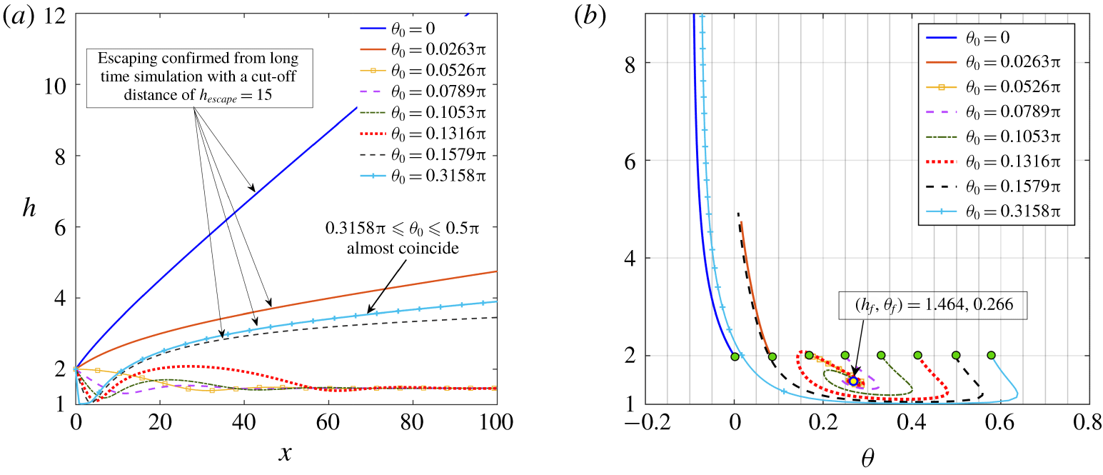
Figure 10. Trajectory of a puller squirmer with $\unicode[STIX]{x1D6FD}=5$
and a wall slip length
$\unicode[STIX]{x1D6FD}=5$
and a wall slip length $l_{S}=0.03$
for various initial orientations
$l_{S}=0.03$
for various initial orientations $(\unicode[STIX]{x1D703}_{0})$
. (a) Trajectory in the
$(\unicode[STIX]{x1D703}_{0})$
. (a) Trajectory in the $(x,h)$
plane and (b) phase plane dynamics,
$(x,h)$
plane and (b) phase plane dynamics, $h$
versus
$h$
versus $\unicode[STIX]{x1D703}$
. In (b), the green circles represent the initial states while the final fixed point for the trapping instances is shown with a black circle.
$\unicode[STIX]{x1D703}$
. In (b), the green circles represent the initial states while the final fixed point for the trapping instances is shown with a black circle.

Figure 11. Increase in detention time for a puller swimmer with $\unicode[STIX]{x1D6FD}=3,\unicode[STIX]{x1D703}_{0}=0.1\unicode[STIX]{x03C0}$
.
$\unicode[STIX]{x1D6FD}=3,\unicode[STIX]{x1D703}_{0}=0.1\unicode[STIX]{x03C0}$
.
Before a full transition of escape to trapping occurs, rising wall slip affects the trajectories by increasing the wall-bound detention time $(T_{det})$
for both pullers and pushers, similar to the previously discussed case of a neutral one. A representative behaviour with
$(T_{det})$
for both pullers and pushers, similar to the previously discussed case of a neutral one. A representative behaviour with $\unicode[STIX]{x1D6FD}=3$
is described in figure 11. In these cases, even after the collision with the wall, the torque on the swimmer is not sufficient to impart a sliding-type motion near the wall. Rather, the swimmer escapes the wall-adjacent region after gliding along the wall for a finite detention time. Thus, the wall-bound detention time of the neutral and puller microswimmers can be controlled by suitably tuning the wall slip length, thus facilitating the formation of bio-aggregates such as biofilms near a wall (Watnick & Kolter Reference Watnick and Kolter2000).
$\unicode[STIX]{x1D6FD}=3$
is described in figure 11. In these cases, even after the collision with the wall, the torque on the swimmer is not sufficient to impart a sliding-type motion near the wall. Rather, the swimmer escapes the wall-adjacent region after gliding along the wall for a finite detention time. Thus, the wall-bound detention time of the neutral and puller microswimmers can be controlled by suitably tuning the wall slip length, thus facilitating the formation of bio-aggregates such as biofilms near a wall (Watnick & Kolter Reference Watnick and Kolter2000).
3.2.3 Pusher squirmer
The swimming states of a pusher swimmer also show wall-bound trapping nature beyond a critical slip length $(l_{s,cr})$
. However, in contrast to pullers, here we find that these stable trapped states exist even for small initial tilt away from the wall, but a further increase of tilt away from the wall results in escaping states only (see figure 12 for an example). In this context, the colliding-escape maps in Shum et al. (Reference Shum, Gaffney and Smith2010) and Pimponi et al. (Reference Pimponi, Chinappi, Gualtieri and Casciola2016) give us information about the trajectories of an E. coli bacterium having properties of a pusher microswimmer (Berke et al.
Reference Berke, Turner, Berg and Lauga2008) near a no-slip and perfect-slip surface. The present results bear resemblance with the reported ones in terms of predicting escaping states for
$(l_{s,cr})$
. However, in contrast to pullers, here we find that these stable trapped states exist even for small initial tilt away from the wall, but a further increase of tilt away from the wall results in escaping states only (see figure 12 for an example). In this context, the colliding-escape maps in Shum et al. (Reference Shum, Gaffney and Smith2010) and Pimponi et al. (Reference Pimponi, Chinappi, Gualtieri and Casciola2016) give us information about the trajectories of an E. coli bacterium having properties of a pusher microswimmer (Berke et al.
Reference Berke, Turner, Berg and Lauga2008) near a no-slip and perfect-slip surface. The present results bear resemblance with the reported ones in terms of predicting escaping states for $\unicode[STIX]{x1D703}_{0}\lesssim 0$
. However, their prediction of colliding trajectories for both surface types with
$\unicode[STIX]{x1D703}_{0}\lesssim 0$
. However, their prediction of colliding trajectories for both surface types with $\unicode[STIX]{x1D703}_{0}\gtrsim 0$
and the absence of stable swimming states for a perfect-slip surface cannot be readily compared with the present results since we have used an additional repulsive force
$\unicode[STIX]{x1D703}_{0}\gtrsim 0$
and the absence of stable swimming states for a perfect-slip surface cannot be readily compared with the present results since we have used an additional repulsive force $(\boldsymbol{F}_{rep})$
near the wall to prevent crashing, a strategy that is also common among others (Spagnolie & Lauga Reference Spagnolie and Lauga2012; Li & Ardekani Reference Li and Ardekani2014; Lintuvuori et al.
Reference Lintuvuori, Brown, Stratford and Marenduzzo2016) for predicting the motion of the microswimmer after collision.
$(\boldsymbol{F}_{rep})$
near the wall to prevent crashing, a strategy that is also common among others (Spagnolie & Lauga Reference Spagnolie and Lauga2012; Li & Ardekani Reference Li and Ardekani2014; Lintuvuori et al.
Reference Lintuvuori, Brown, Stratford and Marenduzzo2016) for predicting the motion of the microswimmer after collision.

Figure 12. Transition of swimming states for a pusher $(\unicode[STIX]{x1D6FD}=-5)$
near a no-slip and slippery wall with
$(\unicode[STIX]{x1D6FD}=-5)$
near a no-slip and slippery wall with $\unicode[STIX]{x1D703}_{0}=-0.165$
. In the inset, the escaping states corresponding a more negative angle,
$\unicode[STIX]{x1D703}_{0}=-0.165$
. In the inset, the escaping states corresponding a more negative angle, $\unicode[STIX]{x1D703}_{0}=-0.248$
, are also shown.
$\unicode[STIX]{x1D703}_{0}=-0.248$
, are also shown.

Figure 13. Critical slip length $(l_{s,cr})$
versus squirmer parameter
$(l_{s,cr})$
versus squirmer parameter $(\unicode[STIX]{x1D6FD})$
for pusher-type swimmers with initial conditions
$(\unicode[STIX]{x1D6FD})$
for pusher-type swimmers with initial conditions $(h_{0},\unicode[STIX]{x1D703}_{0})=(2,0)$
. In the insets (a,b) the transition behaviours are highlighted for
$(h_{0},\unicode[STIX]{x1D703}_{0})=(2,0)$
. In the insets (a,b) the transition behaviours are highlighted for $\unicode[STIX]{x1D6FD}=-5$
and
$\unicode[STIX]{x1D6FD}=-5$
and $-2$
, respectively, while the inset (c) describes the characteristic changes in the periodic oscillations with increasing slip length for
$-2$
, respectively, while the inset (c) describes the characteristic changes in the periodic oscillations with increasing slip length for $\unicode[STIX]{x1D6FD}=-10$
. The onset of transition takes place for
$\unicode[STIX]{x1D6FD}=-10$
. The onset of transition takes place for $\unicode[STIX]{x1D6FD}\sim -1.6$
and is denoted by a ‘blue’ marker.
$\unicode[STIX]{x1D6FD}\sim -1.6$
and is denoted by a ‘blue’ marker.
The non-monotonicity of this critical slip length with initial angular orientations (as shown in figure 8) has not been observed in the case of pushers. Beyond this critical slip length, the swimmer slides along the wall for any initial orientations in the range of $\unicode[STIX]{x1D703}_{0}$
, as discussed above. Figure 13 depicts the consolidated effect of the wall slip on the pusher swimmers for a range of squirmer parameter
$\unicode[STIX]{x1D703}_{0}$
, as discussed above. Figure 13 depicts the consolidated effect of the wall slip on the pusher swimmers for a range of squirmer parameter $-10\leqslant \unicode[STIX]{x1D6FD}\leqslant -2$
. The onset of transition from an escaping to a damped-amplitude oscillation takes place for
$-10\leqslant \unicode[STIX]{x1D6FD}\leqslant -2$
. The onset of transition from an escaping to a damped-amplitude oscillation takes place for $|\unicode[STIX]{x1D6FD}|\sim 1.6$
with a high value of slip length
$|\unicode[STIX]{x1D6FD}|\sim 1.6$
with a high value of slip length $(l_{S})$
. The oscillations become periodic in nature for
$(l_{S})$
. The oscillations become periodic in nature for $|\unicode[STIX]{x1D6FD}|\gtrsim 5$
. This is again opposite to the trend of puller microswimmers, which exhibit periodic and damped-amplitude oscillations for low and high values of the same parameter, respectively. This difference can be related to the contrast in the near-field hydrodynamic effects brought in by the fluid slip at the wall, as discussed in § 3.1. Realization of slip-mediated trapping for pushers with low
$|\unicode[STIX]{x1D6FD}|\gtrsim 5$
. This is again opposite to the trend of puller microswimmers, which exhibit periodic and damped-amplitude oscillations for low and high values of the same parameter, respectively. This difference can be related to the contrast in the near-field hydrodynamic effects brought in by the fluid slip at the wall, as discussed in § 3.1. Realization of slip-mediated trapping for pushers with low $|\unicode[STIX]{x1D6FD}|$
is of utmost importance in view of their non-existence near a no-slip wall.
$|\unicode[STIX]{x1D6FD}|$
is of utmost importance in view of their non-existence near a no-slip wall.
For a significantly high strength of $|\unicode[STIX]{x1D6FD}|$
, the periodic oscillations are present even in the absence of wall slip, as illustrated for
$|\unicode[STIX]{x1D6FD}|$
, the periodic oscillations are present even in the absence of wall slip, as illustrated for $\unicode[STIX]{x1D6FD}=-10$
in the inset (c) of figure 13. Here also, the slip has an important role to play in the form of increasing the frequency of oscillatory height and reducing their amplitudes. This, in turn, allows the swimmer to slide along the wall, maintaining a minimal wall separation as dictated by the balance of the wall repulsive force and the hydrodynamic force for a high slip length.
$\unicode[STIX]{x1D6FD}=-10$
in the inset (c) of figure 13. Here also, the slip has an important role to play in the form of increasing the frequency of oscillatory height and reducing their amplitudes. This, in turn, allows the swimmer to slide along the wall, maintaining a minimal wall separation as dictated by the balance of the wall repulsive force and the hydrodynamic force for a high slip length.
Starting from the same initial orientation, during the final states of a damped cyclic swimming, the puller swimmers point towards the wall (quantified by a positive angle) while pushers show the opposite trend (please refer to figure 14
a). This difference in sign (but not exactly opposite in magnitude) can be attributed to the differences in the physical mechanisms providing the reorientation torque during the trapping states and deciding the actual orientation angle at a particular height, which was also shown to give rise to different rotation rates for the two types of swimmers, as described in figure 2(c,f). It may be counter-intuitive to observe that a pusher swimmer is attracted towards the wall during the oscillations even though it points its director away from the wall $(\unicode[STIX]{x1D703}<0)$
(in figure 14
a). An analogous scenario was reported by Lintuvuori et al. (Reference Lintuvuori, Brown, Stratford and Marenduzzo2016) for a pusher near a no-slip wall. Figure 14(b) depicts the flow field at the end state location of the pusher trajectory. The distortion in the flow field around the microswimmer is observed to be severely altered in the presence of a slippery wall. As a consequence, figure 14(c) shows that, even for negative pitch angles, there exist situations where the thrust force remains negative, i.e. the swimmer gets attracted towards the wall. With subsequent decaying of the amplitudes of oscillation, the microswimmer finally reaches a critical location
$(\unicode[STIX]{x1D703}<0)$
(in figure 14
a). An analogous scenario was reported by Lintuvuori et al. (Reference Lintuvuori, Brown, Stratford and Marenduzzo2016) for a pusher near a no-slip wall. Figure 14(b) depicts the flow field at the end state location of the pusher trajectory. The distortion in the flow field around the microswimmer is observed to be severely altered in the presence of a slippery wall. As a consequence, figure 14(c) shows that, even for negative pitch angles, there exist situations where the thrust force remains negative, i.e. the swimmer gets attracted towards the wall. With subsequent decaying of the amplitudes of oscillation, the microswimmer finally reaches a critical location $(h,\unicode[STIX]{x1D703})\approx (1.110,-0.267)$
where the thrust force
$(h,\unicode[STIX]{x1D703})\approx (1.110,-0.267)$
where the thrust force $(F_{z}^{(Thrust)})$
becomes zero and it does not move further in the vertical direction.
$(F_{z}^{(Thrust)})$
becomes zero and it does not move further in the vertical direction.
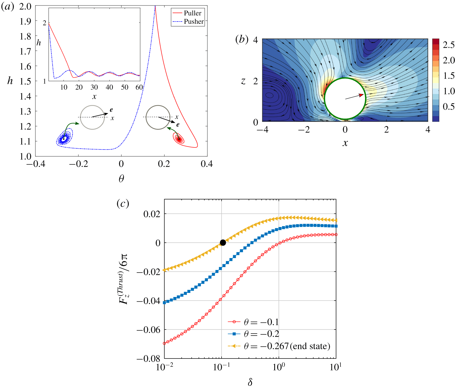
Figure 14. (a) Phase-space trajectory comparison for puller and pusher microswimmers. The parameters are $\unicode[STIX]{x1D6FF}_{0}=1$
,
$\unicode[STIX]{x1D6FF}_{0}=1$
, $\unicode[STIX]{x1D703}_{0}=0.05\unicode[STIX]{x03C0}$
,
$\unicode[STIX]{x1D703}_{0}=0.05\unicode[STIX]{x03C0}$
, $l_{S}=0.55$
and
$l_{S}=0.55$
and $|\unicode[STIX]{x1D6FD}|=4$
. In the inset, the trajectories are compared in the
$|\unicode[STIX]{x1D6FD}|=4$
. In the inset, the trajectories are compared in the $(x,h)$
plane. Swimmer orientations during the final steady-state swimming are also described schematically. (b) The laboratory-frame flow field around the pusher at this end state point in the trajectory. (c) Vertical thrust force variation with distance from the wall at different negative pitch angles attained by the pusher in the trajectory of panel (a). The black filled circle indicates the end state point in the trajectory.
$(x,h)$
plane. Swimmer orientations during the final steady-state swimming are also described schematically. (b) The laboratory-frame flow field around the pusher at this end state point in the trajectory. (c) Vertical thrust force variation with distance from the wall at different negative pitch angles attained by the pusher in the trajectory of panel (a). The black filled circle indicates the end state point in the trajectory.
The slip-modulated wall-bound motion of squirmers shares a characteristic feature with the recent experimental investigation of Ketzetzi et al. (Reference Ketzetzi, de Graaf, Doherty and Kraft2020), who found a prominent tendency of diffusiophoretic Janus colloids to self-propel adjacent to hydrophobic surfaces having high slip lengths and to occasionally leave the surface followed by a steady swimming in wall proximity. In view of the similarity of the surrounding flow patterns in an unbounded domain, the behaviour of such chemically active synthetic particles has been previously mapped onto the squirmer model (Michelin & Lauga Reference Michelin and Lauga2014). However, near a confinement, the distribution of the chemical species around a self-diffusiophoretic particle gets modified, which in turn affects the slip velocity at the particle surface (Uspal et al. Reference Uspal, Popescu, Dietrich and Tasinkevych2015b ; Mozaffari et al. Reference Mozaffari, Sharifi-Mood, Koplik and Maldarelli2016), in contrast to the squirmers, which have a prescribed surface velocity. Thus a qualitative matching of the respective swimming states calls for an explicit account of the dependence of hydrodynamics interaction and chemical species distribution (Popescu et al. Reference Popescu, Uspal, Eskandari, Tasinkevych and Dietrich2018).
4 Conclusions and remarks
To summarize, we have adopted a ‘squirmer’ model to mathematically describe the swimming characteristics of micro-organisms near a plane wall with hydrodynamic slippage. In the low-Reynolds-number regime, the governing fluid flow equations are solved by employing an exact solution technique in the bispherical coordinate system and the hydrodynamic slippage at the wall has been modelled using the Navier slip boundary condition. This provided a unified platform to investigate the translational–rotational velocities of a microswimmer in the far-field domain as well as in the near-surface lubrication region.
The results reveal that hydrodynamic slippage mediates the competitive effects of the near-field hydrodynamic drag and propulsive forces. Consequently, the translational and rotational velocities are both altered, sometimes even showing changes in sign, in contrast to the previous theoretical model of the far-field characteristics of a force-dipole swimmer (Lopez & Lauga Reference Lopez and Lauga2014). The pattern and intensity of the slip-induced changes in the swimming kinematics are critically dependent on the squirming modes and the distance of the microswimmer from the wall.
In comparison to the case of a no-slip wall, near-wall slip reduces the critical value of the dimensionless strength of the second squirming mode required to exert a sufficient hydrodynamic torque enabling a transformation of an escaping microswimmer trajectory to a wall trapping one. Thus wall slip triggers a robust trapping nature of near-surface swimming states. Interestingly, depending upon the launching orientation angle and the strength of the swimming gait, the slip-induced trapping can become either a periodic oscillation or a damped-amplitude oscillations with a final fixed height and orientation. However, in contrast to pullers, for which the critical slip length non-monotonically depends on the initial orientation angle, the critical slip length for pushers is independent of the initial orientation angle. In addition, the maximum attained height, the average height of the periodic oscillations and the final stable height, all get decreased with enhanced slip length.
We have identified that neutral swimmers do not show any tendency to get entrapped near a slippery wall; however, their detention time faces a significant enhancement with increasing wall slip, and their minimum wall separation distance gets reduced before the wall escape takes place. Additionally, as the slip length increases, the critical release orientation of the swimmer director for the transition from scattering to wall collision becomes more pointed away from the wall and finally reaches an asymptotic value.
The present results may turn out to be elemental in providing a theoretical understanding of the complex behaviour either of natural microswimmers near a confinement boundary in a biophysical environment or of artificial swimmers in a controlled lab-on-a-chip device. The above analysis based on uniform surface slip is immediately applicable for conditions where the substrate has a coating of self-assembled monolayers of hydrophobic molecules on atomically smooth surfaces and the sliding of the first layers of molecules takes place giving rise to a phenomenon called ‘intrinsic slippage’ (Huang et al. Reference Huang, Sendner, Horinek, Netz and Bocquet2008; Sega et al. Reference Sega, Sbragaglia, Biferale and Succi2013; Gentili et al. Reference Gentili, Bolognesi, Giacomello, Chinappi and Casciola2014).
However, it is worth mentioning that the present results with high slip length in the micrometre scale are to be used with caution when the characteristic length of the surface asperities of a nano-engineered surface $(\tilde{l}_{a})$
also span over the identical regime, i.e.
$(\tilde{l}_{a})$
also span over the identical regime, i.e. $\tilde{l}_{a}\sim \tilde{l}_{S}$
(Choi & Kim Reference Choi and Kim2006; Joseph et al.
Reference Joseph, Cottin-Bizonne, Benoit, Ybert, Journet, Tabeling and Bocquet2006). In that case an elaborate consideration of the slip length variation along the wall may become inevitable (Ybert et al.
Reference Ybert, Barentin, Cottin-Bizonne, Joseph and Bocquet2007; Asmolov et al.
Reference Asmolov, Zhou, Schmid and Vinogradova2013), especially when the microswimmer goes very close to the wall, i.e.
$\tilde{l}_{a}\sim \tilde{l}_{S}$
(Choi & Kim Reference Choi and Kim2006; Joseph et al.
Reference Joseph, Cottin-Bizonne, Benoit, Ybert, Journet, Tabeling and Bocquet2006). In that case an elaborate consideration of the slip length variation along the wall may become inevitable (Ybert et al.
Reference Ybert, Barentin, Cottin-Bizonne, Joseph and Bocquet2007; Asmolov et al.
Reference Asmolov, Zhou, Schmid and Vinogradova2013), especially when the microswimmer goes very close to the wall, i.e. $\unicode[STIX]{x1D6FF}<l_{S}$
. Researchers have found the significant role of the actual features of a superhydrophobic wall in influencing the motion of particles, both passive or self-propelled, when the particle is very close to the wall (Pimponi et al.
Reference Pimponi, Chinappi, Gualtieri and Casciola2014; Hu et al.
Reference Hu, Wysocki, Winkler and Gompper2015; Nizkaya et al.
Reference Nizkaya, Asmolov, Zhou, Schmid and Vinogradova2015, Reference Nizkaya, Asmolov, Harting and Vinogradova2020). On the other hand, molecular simulations have predicted that specially structured surfaces with nanometre scale roughness can also lead to superhydrophobicity (Lundgren, Allan & Cosgrove Reference Lundgren, Allan and Cosgrove2007; Yang, Tartaglino & Persson Reference Yang, Tartaglino and Persson2008; Koishi et al.
Reference Koishi, Yasuoka, Fujikawa, Ebisuzaki and Zeng2009; Daub et al.
Reference Daub, Wang, Kudesia, Bratko and Luzar2010), a situation that broadens the applicability of the present research. Experimental verification of the present results can be truly intriguing. A major challenge, however, is to realize a pre-designed pattern of wall slip and probe the near-wall dynamics of micro-organisms under the influence of the same by high-resolution microscopy. This may be taken up as a novel research agenda in this field.
$\unicode[STIX]{x1D6FF}<l_{S}$
. Researchers have found the significant role of the actual features of a superhydrophobic wall in influencing the motion of particles, both passive or self-propelled, when the particle is very close to the wall (Pimponi et al.
Reference Pimponi, Chinappi, Gualtieri and Casciola2014; Hu et al.
Reference Hu, Wysocki, Winkler and Gompper2015; Nizkaya et al.
Reference Nizkaya, Asmolov, Zhou, Schmid and Vinogradova2015, Reference Nizkaya, Asmolov, Harting and Vinogradova2020). On the other hand, molecular simulations have predicted that specially structured surfaces with nanometre scale roughness can also lead to superhydrophobicity (Lundgren, Allan & Cosgrove Reference Lundgren, Allan and Cosgrove2007; Yang, Tartaglino & Persson Reference Yang, Tartaglino and Persson2008; Koishi et al.
Reference Koishi, Yasuoka, Fujikawa, Ebisuzaki and Zeng2009; Daub et al.
Reference Daub, Wang, Kudesia, Bratko and Luzar2010), a situation that broadens the applicability of the present research. Experimental verification of the present results can be truly intriguing. A major challenge, however, is to realize a pre-designed pattern of wall slip and probe the near-wall dynamics of micro-organisms under the influence of the same by high-resolution microscopy. This may be taken up as a novel research agenda in this field.
Moreover, beyond the presently adopted spherical squirmer model of micro-organisms, the inclusion of higher-order squirming modes (Pak & Lauga Reference Pak and Lauga2014) will be of interest to the community. It may also be stimulating research directions to additionally inspect the various aspects of microswimming, such as elongated shape of micro-organisms (Shum et al. Reference Shum, Gaffney and Smith2010; Ishimoto & Gaffney Reference Ishimoto and Gaffney2013), direct flagellar contact dynamics (Kantsler et al. Reference Kantsler, Dunkel, Polin and Goldstein2013) or the existence of thermal noise (Li & Tang Reference Li and Tang2009; Drescher et al. Reference Drescher, Dunkel, Cisneros, Ganguly and Goldstein2011; Schaar, Zöttl & Stark Reference Schaar, Zöttl and Stark2015).
Acknowledgements
A.P. would like to acknowledge V. A. Shaik and G. Naveen Kumar for useful discussions. S.C. acknowledges the Department of Science and Technology, Government of India, for a Sir J. C. Bose National Fellowship.
Declaration of interests
The authors report no conflict of interest.
Appendix A. Relation between bispherical and cylindrical coordinates
This relation is shown diagrammatically in figure 15.

Figure 15. The bispherical $(\unicode[STIX]{x1D709},\unicode[STIX]{x1D702},\unicode[STIX]{x1D719})$
coordinate system in relation to the cylindrical coordinates
$(\unicode[STIX]{x1D709},\unicode[STIX]{x1D702},\unicode[STIX]{x1D719})$
coordinate system in relation to the cylindrical coordinates $(\unicode[STIX]{x1D70C},z,\unicode[STIX]{x1D719})$
used in the problem. Since we have
$(\unicode[STIX]{x1D70C},z,\unicode[STIX]{x1D719})$
used in the problem. Since we have $\unicode[STIX]{x1D719}=0$
for this problem, the
$\unicode[STIX]{x1D719}=0$
for this problem, the $x$
axis of the Cartesian reference frame coincides with the
$x$
axis of the Cartesian reference frame coincides with the $\unicode[STIX]{x1D70C}$
axis of the cylindrical coordinate system.
$\unicode[STIX]{x1D70C}$
axis of the cylindrical coordinate system.
Appendix B. Details of the solution procedure
Following Lee & Leal (Reference Lee and Leal1980) the expressions of the pressure and velocity field of the fluid in the cylindrical coordinates $(u,v,w)$
in terms of eigenfunctions in the bispherical coordinates are given by
$(u,v,w)$
in terms of eigenfunctions in the bispherical coordinates are given by
 $$\begin{eqnarray}\displaystyle & \displaystyle p=\mathop{\sum }_{m=0}^{\infty }p_{m}(\unicode[STIX]{x1D709},\unicode[STIX]{x1D702})\cos (m\unicode[STIX]{x1D719}+\unicode[STIX]{x1D6FC}_{m}), & \displaystyle\end{eqnarray}$$
 $$\begin{eqnarray}\displaystyle & \displaystyle p_{m}=\frac{1}{c}\sqrt{(\cosh (\unicode[STIX]{x1D709})-\unicode[STIX]{x1D701})}\mathop{\sum }_{n=m}^{\infty }[A_{n}^{m}\sinh (\unicode[STIX]{x1D6FD}_{n}\unicode[STIX]{x1D709})+B_{n}^{m}\cosh (\unicode[STIX]{x1D6FD}_{n}\unicode[STIX]{x1D709})]P_{n}^{m}(\unicode[STIX]{x1D701}), & \displaystyle\end{eqnarray}$$
 $$\begin{eqnarray}\displaystyle & \displaystyle u=\frac{\unicode[STIX]{x1D70C}p}{2}+u_{0}\cos (\unicode[STIX]{x1D6FC}_{0})+\frac{1}{2}\mathop{\sum }_{m=1}^{\infty }(\unicode[STIX]{x1D6FE}_{m}+\unicode[STIX]{x1D709}_{m})\cos (m\unicode[STIX]{x1D719}+\unicode[STIX]{x1D6FC}_{m}), & \displaystyle\end{eqnarray}$$
 $$\begin{eqnarray}\displaystyle & \displaystyle v=v_{0}\sin (\unicode[STIX]{x1D6FC}_{0})+\mathop{\sum }_{m=1}^{\infty }(\unicode[STIX]{x1D6FE}_{m}-\unicode[STIX]{x1D709}_{m})\sin (m\unicode[STIX]{x1D719}+\unicode[STIX]{x1D6FC}_{m}), & \displaystyle\end{eqnarray}$$
 $$\begin{eqnarray}\displaystyle & \displaystyle w=\frac{zp}{2}+\mathop{\sum }_{m=0}^{\infty }w_{m}\cos (m\unicode[STIX]{x1D719}+\unicode[STIX]{x1D6FC}_{m}). & \displaystyle\end{eqnarray}$$
Here $P_{n}^{m}$
is the associated Legendre polynomial of the first kind,
$P_{n}^{m}$
is the associated Legendre polynomial of the first kind, $\unicode[STIX]{x1D701}=\cos (\unicode[STIX]{x1D702})$
and
$\unicode[STIX]{x1D701}=\cos (\unicode[STIX]{x1D702})$
and $\unicode[STIX]{x1D6FD}_{n}=n+1/2$
. Also
$\unicode[STIX]{x1D6FD}_{n}=n+1/2$
. Also
 $$\begin{eqnarray}\displaystyle & \displaystyle u_{0}=\sqrt{\cosh (\unicode[STIX]{x1D709})-\unicode[STIX]{x1D701}}\mathop{\sum }_{n=1}^{\infty }[E_{n}^{0}\sin (\unicode[STIX]{x1D6FD}_{n}\unicode[STIX]{x1D709})+F_{n}^{0}\cosh (\unicode[STIX]{x1D6FD}_{n}\unicode[STIX]{x1D709})]P_{n}^{1}(\unicode[STIX]{x1D701}), & \displaystyle\end{eqnarray}$$
 $$\begin{eqnarray}\displaystyle & \displaystyle v_{0}=\sqrt{\cosh (\unicode[STIX]{x1D709})-\unicode[STIX]{x1D701}}\mathop{\sum }_{n=1}^{\infty }[G_{n}^{0}\sin (\unicode[STIX]{x1D6FD}_{n}\unicode[STIX]{x1D709})+H_{n}^{0}\cosh (\unicode[STIX]{x1D6FD}_{n}\unicode[STIX]{x1D709})]P_{n}^{1}(\unicode[STIX]{x1D701}), & \displaystyle\end{eqnarray}$$
 $$\begin{eqnarray}\displaystyle & \displaystyle \unicode[STIX]{x1D6FE}_{m}=\sqrt{\cosh (\unicode[STIX]{x1D709})-\unicode[STIX]{x1D701}}\mathop{\sum }_{n=m+1}^{\infty }[E_{n}^{m}\sin (\unicode[STIX]{x1D6FD}_{n}\unicode[STIX]{x1D709})+F_{n}^{m}\cosh (\unicode[STIX]{x1D6FD}_{n}\unicode[STIX]{x1D709})]P_{n}^{m+1}(\unicode[STIX]{x1D701}), & \displaystyle\end{eqnarray}$$
 $$\begin{eqnarray}\displaystyle & \displaystyle \unicode[STIX]{x1D712}_{m}=\sqrt{\cosh (\unicode[STIX]{x1D709})-\unicode[STIX]{x1D701}}\mathop{\sum }_{n=m-1}^{\infty }[G_{n}^{m}\sin (\unicode[STIX]{x1D6FD}_{n}\unicode[STIX]{x1D709})+H_{n}^{m}\cosh (\unicode[STIX]{x1D6FD}_{n}\unicode[STIX]{x1D709})]P_{n}^{m-1}(\unicode[STIX]{x1D701}), & \displaystyle\end{eqnarray}$$
 $$\begin{eqnarray}\displaystyle & \displaystyle w_{m}=\sqrt{\cosh (\unicode[STIX]{x1D709})-\unicode[STIX]{x1D701}}\mathop{\sum }_{n=m}^{\infty }[C_{n}^{m}\sin (\unicode[STIX]{x1D6FD}_{n}\unicode[STIX]{x1D709})]P_{n}^{m}(\unicode[STIX]{x1D701}). & \displaystyle\end{eqnarray}$$
The seven unknown constants ( $A_{n}^{m},B_{n}^{m},C_{n}^{m},E_{n}^{m},F_{n}^{m},G_{n}^{m},H_{m}^{n}$
) appearing in the above expressions are obtained by satisfying the boundary conditions at the swimmer surface (2.4), the Navier slip condition at the plane wall (2.8) and the continuity equation.
$A_{n}^{m},B_{n}^{m},C_{n}^{m},E_{n}^{m},F_{n}^{m},G_{n}^{m},H_{m}^{n}$
) appearing in the above expressions are obtained by satisfying the boundary conditions at the swimmer surface (2.4), the Navier slip condition at the plane wall (2.8) and the continuity equation.
In order to apply the swimmer surface boundary condition (2.4), the surface velocity components are expanded in terms of bispherical eigenfunctions as given below:
 $$\begin{eqnarray}\displaystyle & \displaystyle u_{s}=\mathop{\sum }_{m}u_{s}^{m}(\unicode[STIX]{x1D709},\unicode[STIX]{x1D702})\cos (m\unicode[STIX]{x1D719}+\unicode[STIX]{x1D6FC}_{m}), & \displaystyle\end{eqnarray}$$
 $$\begin{eqnarray}\displaystyle & \displaystyle v_{s}=\mathop{\sum }_{m}v_{s}^{m}(\unicode[STIX]{x1D709},\unicode[STIX]{x1D702})\sin (m\unicode[STIX]{x1D719}+\unicode[STIX]{x1D6FC}_{m}), & \displaystyle\end{eqnarray}$$
 $$\begin{eqnarray}\displaystyle & \displaystyle w_{s}=\mathop{\sum }_{m}w_{s}^{m}(\unicode[STIX]{x1D709},\unicode[STIX]{x1D702})\cos (m\unicode[STIX]{x1D719}+\unicode[STIX]{x1D6FC}_{m}), & \displaystyle\end{eqnarray}$$
where for $m=0$
,
$m=0$
,
 $$\begin{eqnarray}\displaystyle & \displaystyle u_{s}^{0}=\sqrt{\cosh (\unicode[STIX]{x1D709}_{0})-\unicode[STIX]{x1D701}}\sum \mathop{X}_{n}^{0}(\unicode[STIX]{x1D709})P_{n}^{1}(\unicode[STIX]{x1D701}), & \displaystyle\end{eqnarray}$$
 $$\begin{eqnarray}\displaystyle & \displaystyle v_{s}^{0}=\sqrt{\cosh (\unicode[STIX]{x1D709}_{0})-\unicode[STIX]{x1D701}}\sum \mathop{Y}_{n}^{0}(\unicode[STIX]{x1D709})P_{n}^{1}(\unicode[STIX]{x1D701}), & \displaystyle\end{eqnarray}$$ $m\geqslant 1$
,
$m\geqslant 1$
,  $$\begin{eqnarray}\displaystyle & \displaystyle u_{s}^{m}+v_{s}^{m}=\sqrt{\cosh (\unicode[STIX]{x1D709}_{0})-\unicode[STIX]{x1D701}}\sum \mathop{X}_{n}^{m}(\unicode[STIX]{x1D709})P_{n}^{m+1}(\unicode[STIX]{x1D701}), & \displaystyle\end{eqnarray}$$
 $$\begin{eqnarray}\displaystyle & \displaystyle u_{s}^{m}-v_{s}^{m}=\sqrt{\cosh (\unicode[STIX]{x1D709}_{0})-\unicode[STIX]{x1D701}}\sum \mathop{Y}_{n}^{m}(\unicode[STIX]{x1D709})P_{n}^{m-1}(\unicode[STIX]{x1D701}), & \displaystyle\end{eqnarray}$$ $m$
,
$m$
,  $$\begin{eqnarray}w_{s}^{m}=\sqrt{\cosh (\unicode[STIX]{x1D709}_{0})-\unicode[STIX]{x1D701}}\sum \mathop{Z}_{n}^{m}(\unicode[STIX]{x1D709})P_{n}^{m}(\unicode[STIX]{x1D701}).\end{eqnarray}$$
The constants $X_{n}^{m}$
,
$X_{n}^{m}$
, $Y_{n}^{m}$
and
$Y_{n}^{m}$
and $Z_{n}^{m}$
are to be determined by using the boundary condition on the swimmer surface. Now making use of the orthogonality of the associated Legendre polynomials, we obtain an infinite set of linear algebraic equations involving the unknown constants. Since the values of these constants decay with increasing values of
$Z_{n}^{m}$
are to be determined by using the boundary condition on the swimmer surface. Now making use of the orthogonality of the associated Legendre polynomials, we obtain an infinite set of linear algebraic equations involving the unknown constants. Since the values of these constants decay with increasing values of $n$
, we truncate the algebraic system of equations for a large number of terms
$n$
, we truncate the algebraic system of equations for a large number of terms $N$
so that the error in evaluating these constants (
$N$
so that the error in evaluating these constants ( $A_{n}^{m},B_{n}^{m},C_{n}^{m},E_{n}^{m},F_{n}^{m},G_{n}^{m},H_{m}^{n}$
) as well as the swimmer velocity components
$A_{n}^{m},B_{n}^{m},C_{n}^{m},E_{n}^{m},F_{n}^{m},G_{n}^{m},H_{m}^{n}$
) as well as the swimmer velocity components $(V_{x},V_{z},\unicode[STIX]{x1D6FA}_{y})$
between steps
$(V_{x},V_{z},\unicode[STIX]{x1D6FA}_{y})$
between steps $N$
and
$N$
and $N+1$
becomes
$N+1$
becomes ${\leqslant}10^{-6}$
. The system of equations has a banded matrix structure
${\leqslant}10^{-6}$
. The system of equations has a banded matrix structure $(7N\times 7N)$
and was solved using the default matrix solver in MATLAB. It automatically switches to an appropriate solver based on the symmetries in the matrix structure and therefore minimizes the computational time.
$(7N\times 7N)$
and was solved using the default matrix solver in MATLAB. It automatically switches to an appropriate solver based on the symmetries in the matrix structure and therefore minimizes the computational time.

Figure 16. Convergence of translational and rotational velocity of the microswimmer with number of terms used for series truncation $(N)$
. Here we have chosen the most computationally demanding situation with
$(N)$
. Here we have chosen the most computationally demanding situation with $l_{S}=10$
and
$l_{S}=10$
and $\unicode[STIX]{x1D6FF}=0.01$
. Other parameters are the same as in figures 2(a), 2(b) and 2(c), respectively.
$\unicode[STIX]{x1D6FF}=0.01$
. Other parameters are the same as in figures 2(a), 2(b) and 2(c), respectively.
Similar to the previous works related to a passive or active sphere moving near a no-slip wall, we also find that the decay of these constants becomes very slow as the swimmer comes close to the plane wall, which calls for a large number of terms to be retained to reach the desired accuracy (Lee & Leal Reference Lee and Leal1980; Yazdi & Borhan Reference Yazdi and Borhan2017). Adding to this, the increased value of the slip length at the plane wall turns out to be another hurdle to obtain a uniform accuracy throughout the calculations (Kezirian Reference Kezirian1992; Loussaief et al.
Reference Loussaief, Pasol and Feuillebois2015). Thus, for extreme cases when the swimmer is very close to wall (e.g. $h<1.05$
) and at the same time the wall slip length is very high (e.g.
$h<1.05$
) and at the same time the wall slip length is very high (e.g. $l_{S}>5$
), we work with an accuracy of
$l_{S}>5$
), we work with an accuracy of $10^{-4}$
to save on the computational cost. To gain confidence on the results with
$10^{-4}$
to save on the computational cost. To gain confidence on the results with $10^{-4}$
accuracy, we have checked the constant coefficients as well as velocity magnitudes for three different swimmer types with the most extreme cases considered, i.e.
$10^{-4}$
accuracy, we have checked the constant coefficients as well as velocity magnitudes for three different swimmer types with the most extreme cases considered, i.e. $h=1.01$
and
$h=1.01$
and $l_{S}=10$
. Some typical examples have been provided in figure 16. These depict that upon a gradual increase of the number of terms
$l_{S}=10$
. Some typical examples have been provided in figure 16. These depict that upon a gradual increase of the number of terms $(N)$
, the translational and rotational velocities of the microswimmer show only a minimal variation after a critical
$(N)$
, the translational and rotational velocities of the microswimmer show only a minimal variation after a critical $N$
is reached. Following this, we have kept a sufficiently high number of terms in the series beyond which the velocity magnitudes differ only after four significant digits, i.e. an accuracy of
$N$
is reached. Following this, we have kept a sufficiently high number of terms in the series beyond which the velocity magnitudes differ only after four significant digits, i.e. an accuracy of $10^{-4}$
. In addition we have confirmed that the relative percentage error for the velocity calculations (e.g.
$10^{-4}$
. In addition we have confirmed that the relative percentage error for the velocity calculations (e.g. $|(V_{x}^{(N+1)}-V_{x}^{(N)})/V_{x}^{(N)}|\times 100\,\%$
) remains
$|(V_{x}^{(N+1)}-V_{x}^{(N)})/V_{x}^{(N)}|\times 100\,\%$
) remains ${<}0.01\,\%$
. A similar strategy to work with different accuracies for different distances from the wall is quite common in problems where a similar semi-analytical technique has been employed (Tabatabaei & Van De Ven Reference Tabatabaei and Van De Ven2010).
${<}0.01\,\%$
. A similar strategy to work with different accuracies for different distances from the wall is quite common in problems where a similar semi-analytical technique has been employed (Tabatabaei & Van De Ven Reference Tabatabaei and Van De Ven2010).
In addition, we have chosen a very high relative tolerance of $10^{-8}$
in the MATLAB ODE45 solver employed for obtaining the quasi-steady-state trajectories presented in the paper. This solver is advantageous since it can adaptively vary the time steps to meet the required tolerance by employing a six-stage fifth-order Runge–Kutta scheme. As a final confirmation of the working accuracy of the translational and rotational velocities, we have compared the microswimmer trajectories for representative cases and found no distinguishable change.
$10^{-8}$
in the MATLAB ODE45 solver employed for obtaining the quasi-steady-state trajectories presented in the paper. This solver is advantageous since it can adaptively vary the time steps to meet the required tolerance by employing a six-stage fifth-order Runge–Kutta scheme. As a final confirmation of the working accuracy of the translational and rotational velocities, we have compared the microswimmer trajectories for representative cases and found no distinguishable change.
Appendix C. Decomposition into fundamental Stokesian subproblems
Owing to the linearity of the Stokes equation, the flow field generated by the motion a passively moving particle can be obtained by superposing the individual flow fields due to fundamental modes of the associated kinematics. Along similar lines, in the present problem of self-propulsion, the flow fields due to the motion of a spherical particle with $V_{x},V_{z},\unicode[STIX]{x1D6FA}_{y}$
in an otherwise quiescent fluid and that due to tangential slip velocity specified by the squirming modes
$V_{x},V_{z},\unicode[STIX]{x1D6FA}_{y}$
in an otherwise quiescent fluid and that due to tangential slip velocity specified by the squirming modes $(B_{1},B_{2})$
for the case of a stationary sphere, each with a Navier slip condition at the plane wall, are sufficient to fully characterize the problem. In subsequent discussions, we denote each of these flow fields as ‘fundamental problems’. Expressions of different terms in (2.9) are obtained from these fundamental problems as detailed below.
$(B_{1},B_{2})$
for the case of a stationary sphere, each with a Navier slip condition at the plane wall, are sufficient to fully characterize the problem. In subsequent discussions, we denote each of these flow fields as ‘fundamental problems’. Expressions of different terms in (2.9) are obtained from these fundamental problems as detailed below.
Subproblem A – A stationary spherical particle under the action of tangential slip velocity due to squirming:
Here the sphere is fixed in space but the surface slip flow due to the squirming action leads to the following components of thrust force and torque components.
-
(i) Thrust force along the $z$
direction: (C 1)
$$\begin{eqnarray}F_{z}^{(Thrust)}=-2\sqrt{2}\unicode[STIX]{x03C0}\sinh (\unicode[STIX]{x1D709}_{0})\mathop{\sum }_{n=0}^{\infty }\left[C_{n}^{0}-\left(n+\frac{1}{2}\right)(A_{n}^{0}-B_{n}^{0})\right].\end{eqnarray}$$
$z$
direction: (C 1)
$$\begin{eqnarray}F_{z}^{(Thrust)}=-2\sqrt{2}\unicode[STIX]{x03C0}\sinh (\unicode[STIX]{x1D709}_{0})\mathop{\sum }_{n=0}^{\infty }\left[C_{n}^{0}-\left(n+\frac{1}{2}\right)(A_{n}^{0}-B_{n}^{0})\right].\end{eqnarray}$$
-
(ii) Thrust force along the
$x$
direction: (C 2)
$$\begin{eqnarray}F_{x}^{(Thrust)}=-\sqrt{2}\unicode[STIX]{x03C0}\sinh (\unicode[STIX]{x1D709}_{0})\mathop{\sum }_{n=0}^{\infty }[G_{n}^{1}-H_{n}^{1}+n(n+1)(A_{n}^{1}-B_{n}^{1})].\end{eqnarray}$$
-
(iii) Thrust torque along the
$y$
direction: (C 3)
$$\begin{eqnarray}\displaystyle T_{y}^{(Thrust)} & = & \displaystyle \sqrt{2}\unicode[STIX]{x03C0}\sinh ^{2}(\unicode[STIX]{x1D709}_{0})\mathop{\sum }_{n=0}^{\infty }[\!\text{coth}(\unicode[STIX]{x1D709}_{0})\{n(n+1)(A_{n}^{1}-B_{n}^{1})+(G_{n}^{1}-H_{n}^{1})\}\nonumber\\ \displaystyle & & \displaystyle -\,2n(n+1)C_{n}^{1}-(2n+1)(G_{n}^{1}-H_{n}^{1})\!].\end{eqnarray}$$


Subproblem B – Translation of a non-rotating spherical particle perpendicular to the wall:
Here the problem has an axisymmetric nature about the $z$
axis. Hence we only have
$z$
axis. Hence we only have $m=0$
and
$m=0$
and $\unicode[STIX]{x1D6FC}_{0}=0$
. The particle faces only a vertical drag force but no torque. The resistance factor associated with force along the
$\unicode[STIX]{x1D6FC}_{0}=0$
. The particle faces only a vertical drag force but no torque. The resistance factor associated with force along the $z$
direction is given by (Lee & Leal Reference Lee and Leal1980)
$z$
direction is given by (Lee & Leal Reference Lee and Leal1980)
 $$\begin{eqnarray}f_{z,T}=-2\sqrt{2}\unicode[STIX]{x03C0}\sinh (\unicode[STIX]{x1D709}_{0})\mathop{\sum }_{n=0}^{\infty }\left[C_{n}^{0}-\left(n+\frac{1}{2}\right)(A_{n}^{0}-B_{n}^{0})\right].\end{eqnarray}$$
Subproblem C – Translation of a non-rotating spherical particle parallel to the wall:
In this case the hydrodynamics can be fully described with $m=1$
and
$m=1$
and $\unicode[STIX]{x1D6FC}_{1}=0$
. The sphere experiences both hydrodynamic drag force and torque (O’Neill Reference O’Neill1964; Lee & Leal Reference Lee and Leal1980).
$\unicode[STIX]{x1D6FC}_{1}=0$
. The sphere experiences both hydrodynamic drag force and torque (O’Neill Reference O’Neill1964; Lee & Leal Reference Lee and Leal1980).
-
(i) Resistance factor associated with force along the
$x$
direction: (C 5)
$$\begin{eqnarray}f_{x,T}=-\sqrt{2}\unicode[STIX]{x03C0}\sinh (\unicode[STIX]{x1D709}_{0})\mathop{\sum }_{n=0}^{\infty }[G_{n}^{1}-H_{n}^{1}+n(n+1)(A_{n}^{1}-B_{n}^{1})].\end{eqnarray}$$
-
(ii) Resistance factor associated with torque along the
$y$
direction (O’Neill Reference O’Neill1967): (C 6)
$$\begin{eqnarray}\displaystyle f_{y,T} & = & \displaystyle \sqrt{2}\unicode[STIX]{x03C0}\sinh ^{2}(\unicode[STIX]{x1D709}_{0})\mathop{\sum }_{n=0}^{\infty }[\!\text{coth}(\unicode[STIX]{x1D709}_{0})\{n(n+1)(A_{n}^{1}-B_{n}^{1})+(G_{n}^{1}-H_{n}^{1})\}-2n(n+1)C_{n}^{1}\nonumber\\ \displaystyle & & \displaystyle -\,(2n+1)(G_{n}^{1}-H_{n}^{1})\!].\end{eqnarray}$$


Subproblem D – Rotation of a non-translating spherical particle parallel to the wall:
Similar to the above subproblem, here also only $m=1$
and
$m=1$
and $\unicode[STIX]{x1D6FC}_{1}=0$
terms survive. Apart from a resistance torque to rotation, a wall-parallel force is also exerted by the fluid onto the particle (Dean & O’Neill Reference Dean and O’Neill1963; Lee & Leal Reference Lee and Leal1980).
$\unicode[STIX]{x1D6FC}_{1}=0$
terms survive. Apart from a resistance torque to rotation, a wall-parallel force is also exerted by the fluid onto the particle (Dean & O’Neill Reference Dean and O’Neill1963; Lee & Leal Reference Lee and Leal1980).
-
(i) Resistance factor associated with force along the
$x$
direction: (C 7)
$$\begin{eqnarray}f_{x,R}=-\sqrt{2}\unicode[STIX]{x03C0}\sinh ^{2}(\unicode[STIX]{x1D709}_{0})\mathop{\sum }_{n=0}^{\infty }[G_{n}^{1}-H_{n}^{1}+n(n+1)(A_{n}^{1}-B_{n}^{1})].\end{eqnarray}$$
-
(ii) Resistance factor associated with torque along the
$y$
direction (O’Neill Reference O’Neill1967): (C 8)
$$\begin{eqnarray}\displaystyle f_{y,R} & = & \displaystyle \sqrt{2}\unicode[STIX]{x03C0}\sinh ^{3}(\unicode[STIX]{x1D709}_{0})\mathop{\sum }_{n=0}^{\infty }[\!\text{coth}(\unicode[STIX]{x1D709}_{0})\{n(n+1)(A_{n}^{1}-B_{n}^{1})+(G_{n}^{1}-H_{n}^{1})\}-2n(n+1)C_{n}^{1}\nonumber\\ \displaystyle & & \displaystyle -\,(2n+1)(G_{n}^{1}-H_{n}^{1})\!].\end{eqnarray}$$


The constants $X_{n}^{m}$
,
$X_{n}^{m}$
, $Y_{n}^{m}$
and
$Y_{n}^{m}$
and $Z_{n}^{m}$
in (B 14) and (B 16) come from the boundary condition at the microswimmer surface and thus remain unaffected by the slip at the plane wall. To avoid repetition, we refer the reader to the earlier works (Lee & Leal Reference Lee and Leal1980; Shaik & Ardekani Reference Shaik and Ardekani2017) where these constants are provided for all the fundamental problems involved in the present study. The only difference arises from the fact that they have considered the body to be below the
$Z_{n}^{m}$
in (B 14) and (B 16) come from the boundary condition at the microswimmer surface and thus remain unaffected by the slip at the plane wall. To avoid repetition, we refer the reader to the earlier works (Lee & Leal Reference Lee and Leal1980; Shaik & Ardekani Reference Shaik and Ardekani2017) where these constants are provided for all the fundamental problems involved in the present study. The only difference arises from the fact that they have considered the body to be below the $\unicode[STIX]{x1D709}=0$
surface while we have taken the opposite configuration. The flow fields due to a passive sphere moving near a slippery surface, having translational and rotational velocity components parallel to the surface (e.g.
$\unicode[STIX]{x1D709}=0$
surface while we have taken the opposite configuration. The flow fields due to a passive sphere moving near a slippery surface, having translational and rotational velocity components parallel to the surface (e.g. $V_{x}$
and
$V_{x}$
and $\unicode[STIX]{x1D6FA}_{y}$
), have been obtained previously (Kezirian Reference Kezirian1992; Loussaief et al.
Reference Loussaief, Pasol and Feuillebois2015) using a similar method as described above. However, the problem of a sphere moving normal to a slippery wall has only been solved using the streamfunction approach (Goren Reference Goren1973). The present authors have solved this problem using the direct solution of the Stokes equation as discussed before. In addition, the flow problem due to the tangential squirming modes on the surface of a stationary sphere adjacent to a plane wall with fluid slip has been solved for the first time.
$\unicode[STIX]{x1D6FA}_{y}$
), have been obtained previously (Kezirian Reference Kezirian1992; Loussaief et al.
Reference Loussaief, Pasol and Feuillebois2015) using a similar method as described above. However, the problem of a sphere moving normal to a slippery wall has only been solved using the streamfunction approach (Goren Reference Goren1973). The present authors have solved this problem using the direct solution of the Stokes equation as discussed before. In addition, the flow problem due to the tangential squirming modes on the surface of a stationary sphere adjacent to a plane wall with fluid slip has been solved for the first time.
Appendix D. Reciprocal theorem for a microswimmer near a slippery surface
The propulsive force and torque on the microswimmer can be determined without solving the Stokes equation by utilizing the Reynolds reciprocal theorem between two Stokes flows with the same geometry, which has the general form (Happel & Brenner Reference Happel and Brenner1981)
 $$\begin{eqnarray}\iint _{\unicode[STIX]{x2202}S}\boldsymbol{n}\boldsymbol{\cdot }\unicode[STIX]{x1D748}^{\prime }\boldsymbol{\cdot }\boldsymbol{u}^{\prime \prime }=\iint _{\unicode[STIX]{x2202}S}\boldsymbol{n}\boldsymbol{\cdot }\unicode[STIX]{x1D748}^{\prime \prime }\boldsymbol{\cdot }\boldsymbol{u}^{\prime },\end{eqnarray}$$
where $\boldsymbol{u}^{\prime }$
and
$\boldsymbol{u}^{\prime }$
and $\unicode[STIX]{x1D748}^{\prime }$
correspond to the swimming problem with a tangential squirming velocity and
$\unicode[STIX]{x1D748}^{\prime }$
correspond to the swimming problem with a tangential squirming velocity and $\boldsymbol{u}^{\prime \prime }$
and
$\boldsymbol{u}^{\prime \prime }$
and $\unicode[STIX]{x1D748}^{\prime \prime }$
describe a complementary Stokes problem. Here
$\unicode[STIX]{x1D748}^{\prime \prime }$
describe a complementary Stokes problem. Here $\unicode[STIX]{x2202}S$
is the boundary of the fluid domain.
$\unicode[STIX]{x2202}S$
is the boundary of the fluid domain.
Previous works related to the motion of a microswimmer near a no-slip surface (Crowdy Reference Crowdy2011, Reference Crowdy2013; Mozaffari et al.
Reference Mozaffari, Sharifi-Mood, Koplik and Maldarelli2016) have taken advantage of vanishing fluid velocity at the plane wall to reduce the flow boundary in (D 1) to the swimmer surface only, i.e. $\unicode[STIX]{x2202}S=S_{p}$
. However, it is not the case for a plane wall with a slipping boundary condition and we are left with
$\unicode[STIX]{x2202}S=S_{p}$
. However, it is not the case for a plane wall with a slipping boundary condition and we are left with
 $$\begin{eqnarray}\iint _{S_{p}}\boldsymbol{n}\boldsymbol{\cdot }\unicode[STIX]{x1D748}^{\prime }\boldsymbol{\cdot }\boldsymbol{u}^{\prime \prime }+\underbrace{\iint _{S_{w}}\boldsymbol{n}\boldsymbol{\cdot }\unicode[STIX]{x1D748}^{\prime }\boldsymbol{\cdot }\boldsymbol{u}^{\prime \prime }}_{Wall\;slip\;contribution}=\iint _{S_{p}}\boldsymbol{n}\boldsymbol{\cdot }\unicode[STIX]{x1D748}^{\prime \prime }\boldsymbol{\cdot }\boldsymbol{u}^{\prime }+\underbrace{\iint _{S_{w}}\boldsymbol{n}\boldsymbol{\cdot }\unicode[STIX]{x1D748}^{\prime \prime }\boldsymbol{\cdot }\boldsymbol{u}^{\prime }}_{Wall\;slip\;contribution},\end{eqnarray}$$
where $S_{w}$
is the surface of the slippery plane wall. It was shown (Loussaief et al.
Reference Loussaief, Pasol and Feuillebois2015) that the contributions of the extra terms due to non-vanishing fluid velocity at the plane wall, appearing in both sides of (D 2), become equal, i.e.
$S_{w}$
is the surface of the slippery plane wall. It was shown (Loussaief et al.
Reference Loussaief, Pasol and Feuillebois2015) that the contributions of the extra terms due to non-vanishing fluid velocity at the plane wall, appearing in both sides of (D 2), become equal, i.e.
 $$\begin{eqnarray}\iint _{S_{w}}\boldsymbol{n}\boldsymbol{\cdot }\unicode[STIX]{x1D748}^{\prime }\boldsymbol{\cdot }\boldsymbol{u}^{\prime \prime }=\iint _{S_{w}}\boldsymbol{n}\boldsymbol{\cdot }\unicode[STIX]{x1D748}^{\prime \prime }\boldsymbol{\cdot }\boldsymbol{u}^{\prime },\end{eqnarray}$$
and we subsequently obtain
 $$\begin{eqnarray}\iint _{S_{p}}\boldsymbol{n}\boldsymbol{\cdot }\unicode[STIX]{x1D748}^{\prime }\boldsymbol{\cdot }\boldsymbol{u}^{\prime \prime }=\iint _{S_{p}}\boldsymbol{n}\boldsymbol{\cdot }\unicode[STIX]{x1D748}^{\prime \prime }\boldsymbol{\cdot }\boldsymbol{u}^{\prime }.\end{eqnarray}$$
Next we choose the complementary problem as the motion of a spherical particle near a slippery plane wall where the particle has a translational velocity $\boldsymbol{U}^{\prime \prime }$
and rotational velocity
$\boldsymbol{U}^{\prime \prime }$
and rotational velocity $\unicode[STIX]{x1D734}^{\prime \prime }$
. Utilizing the force- and torque-free conditions of the microswimmer and employing the boundary condition (2.4) on the swimmer surface, finally (D 1) is simplified to
$\unicode[STIX]{x1D734}^{\prime \prime }$
. Utilizing the force- and torque-free conditions of the microswimmer and employing the boundary condition (2.4) on the swimmer surface, finally (D 1) is simplified to
 $$\begin{eqnarray}\boldsymbol{F}^{\prime \prime }\boldsymbol{\cdot }\boldsymbol{U}+\boldsymbol{T}^{\prime \prime }\boldsymbol{\cdot }\unicode[STIX]{x1D734}=-\iint _{S_{p}}\boldsymbol{n}\boldsymbol{\cdot }\unicode[STIX]{x1D748}^{\prime \prime }\boldsymbol{\cdot }\boldsymbol{u}^{s}\,\text{d}S,\end{eqnarray}$$
where $\boldsymbol{F}^{\prime \prime }$
and
$\boldsymbol{F}^{\prime \prime }$
and $\boldsymbol{T}^{\prime \prime }$
represent the force and torque on the spherical particle in the complementary Stokes problem. The above equation suggests that the translational and rotational velocities of the microswimmer can be found by knowing the surface tangential velocity and the solution of the complementary Stokes problem, thereby bypassing the detailed solution of the swimmer problem.
$\boldsymbol{T}^{\prime \prime }$
represent the force and torque on the spherical particle in the complementary Stokes problem. The above equation suggests that the translational and rotational velocities of the microswimmer can be found by knowing the surface tangential velocity and the solution of the complementary Stokes problem, thereby bypassing the detailed solution of the swimmer problem.
Appendix E. Validation of the numerical calculations
The solutions obtained from the numerical codes employed in the present study to obtain the full solution of the Stokes equation were first validated with various earlier works regarding a spherical particle motion near a no-slip surface (Brenner Reference Brenner1961; O’Neill Reference O’Neill1964) as well as near a slippery surface (Goren Reference Goren1973; Kezirian Reference Kezirian1992; Loussaief et al. Reference Loussaief, Pasol and Feuillebois2015). Subsequently the force and torque values obtained from the full Stokes equation solution are rechecked with the aforementioned reciprocal theorem approach (appendix D).

Figure 17. Variation of the squirmer vertical velocity component and rotational velocity with the distance from the wall $(\unicode[STIX]{x1D6FF})$
. In the inset of each panel the log-scale variations are also highlighted. The parameters are
$(\unicode[STIX]{x1D6FF})$
. In the inset of each panel the log-scale variations are also highlighted. The parameters are $B_{1}=1$
,
$B_{1}=1$
, $\unicode[STIX]{x1D6FD}=4$
and
$\unicode[STIX]{x1D6FD}=4$
and $\unicode[STIX]{x1D703}=\unicode[STIX]{x03C0}/8$
.
$\unicode[STIX]{x1D703}=\unicode[STIX]{x03C0}/8$
.

Figure 18. The transition from escape to oscillatory sliding trajectory with increasing slip length. Here short-range repulsive force is not used. The parameters are $\unicode[STIX]{x1D703}_{0}=0.05\unicode[STIX]{x03C0}$
,
$\unicode[STIX]{x1D703}_{0}=0.05\unicode[STIX]{x03C0}$
, $\unicode[STIX]{x1D6FD}=4$
and
$\unicode[STIX]{x1D6FD}=4$
and $h_{0}=2$
.
$h_{0}=2$
.
In figure 17(a,b) we compare the no-slip results of the vertical component of velocity and rotational velocity with the calculations of the reciprocal theorem as well as with the previously reported results of Shaik & Ardekani (Reference Shaik and Ardekani2017). The reciprocal theorem turns out to match almost exactly with the present exact solutions. The slight disagreement of the current results with those of Shaik & Ardekani (Reference Shaik and Ardekani2017) is due to the fact that their results were obtained for a squirmer approaching a two-fluid interface. We have taken their results corresponding to a high value of the viscosity ratio ( $\unicode[STIX]{x1D706}=10$
), which only approximately resembles the characteristics of a no-slip wall (Lee & Leal Reference Lee and Leal1980), while in an ideal case
$\unicode[STIX]{x1D706}=10$
), which only approximately resembles the characteristics of a no-slip wall (Lee & Leal Reference Lee and Leal1980), while in an ideal case $\unicode[STIX]{x1D706}\rightarrow \infty$
is required to recover the results near a no-slip solid wall.
$\unicode[STIX]{x1D706}\rightarrow \infty$
is required to recover the results near a no-slip solid wall.
Appendix F. Verification of slip-induced trapping
This verification is shown diagrammatically in figure 18.


 Open access