


1. Introduction
Basis, the difference between the spot and futures prices, localizes the futures price for a given location and time and is therefore a key component of price risk management (Tomek, Reference Tomek1997; Taylor, Dhuyvetter, and Kastens, Reference Taylor, Dhuyvetter and Kastens2006). If current basis deviates significantly from its historical levels, market participants can address why by inquiring into local market circumstances. Having accurate basis forecasts also aids market participants in hedging with futures contracts by providing an estimate of the prospective price they will receive or pay when they enter into a futures position. Accurate forecasts of basis are also important in timing sales and purchases of commodities as it generates a forecast of expected future cash prices (Tonsor, Dhuyvetter, and Mintert, Reference Tonsor, Dhuyvetter and Mintert2004).
Given the importance of accurate basis information, this study investigates whether basis forecasts can be improved by combining different forecasting models in a Bayesian framework. The earliest studies examining basis forecasts used structural models. For instance, storage and transportation costs, excess local supply, existing stocks, and seasonality are found to affect basis (Martin, Groenewegen, and Pidgeon, Reference Martin, Groenewegen and Pidgeon1980; Garcia and Good, Reference Garcia and Good1983). Moving historical averages, commonly referred to as naïve forecasts, have been the most typical approach to forecast basis (Hauser, Garcia, and Tumblin, Reference Hauser, Garcia and Tumblin1990). When compared with structural models, the naïve models are generally found to predict basis more accurately. A regression of basis on structural variables such as transportation costs and local supply information along with a naïve forecast is found to somewhat improve on the performance of the best naïve model (Jiang and Hayenga, Reference Jiang and Hayenga1997).
The number of years to include in a moving average has been a key issue in the literature. Looking at wheat, corn, milo, and soybeans, Dhuyvetter and Kastens (Reference Dhuyvetter and Kastens1998), for instance, find that longer moving averages work best, whereas Taylor, Dhuyvetter, and Kastens (Reference Taylor, Dhuyvetter and Kastens2006) find shorter moving averages perform better for the same commodities. Hatchett, Brorsen, and Anderson (Reference Hatchett, Brorsen and Anderson2010) conclude that although using shorter moving averages yields better basis forecasts when a market has undergone a structural change, using longer moving averages performs better otherwise.
More complex time-series models such as autoregressive integrated moving average (ARIMA) and vector autoregressive models are found to modestly outperform naïve approaches, but only for short forecast horizons (Sanders and Manfredo, Reference Sanders and Manfredo2006; Sanders and Baker, Reference Sanders and Baker2012). Additionally, some studies indicate basis may be getting harder to predict over time (Irwin et al. Reference Irwin, Garcia, Good and Kunda2009). This observation has led to recent investigations of regime switching models (Sanders and Baker, Reference Sanders and Baker2012); however, these models only perform well over short forecast horizons.
Our study reexamines many variations of models in previous work and gauges their effectiveness at forecasting feeder cattle basis in Georgia. Given the ambiguity in the literature on the best forecasting model of basis and the importance of accurate forecasts of basis for market participants, we take a Bayesian model averaging (BMA) approach. By averaging over different competing forecasting models, BMA incorporates model uncertainty into inferences about parameters and has been shown to improve predictive performance in many instances (Hoeting et al. Reference Hoeting, Madigan, Raftery and Volinsky1999; Koop, Reference Koop2003). The main focus of this research is on evaluating the potential of BMA as a method for producing forecasts that consistently perform well and potentially providing an improvement over current methods of basis forecasts. For this purpose, we consider variations of previously examined models in our BMA framework. Specifically, autoregressive models and regressions on moving historical averages of varying lengths with and without additional fundamental variables such as current market information, transportation costs, and input costs are considered. Each selected model’s forecasting performance is compared with that of naïve forecast and of the forecast obtained with BMA.
Most previous studies on basis forecasting focus on a nearby basis series: basis in a given month is computed with futures contracts that correspond to that month or the nearest months’ contract. This kind of forecast concerns itself primarily with what basis will be in the near future, specifically at the time the nearby contract expires. However, a producer may also be interested in what basis will be in the far distant future when the sale or purchase of products will occur. This type of forecast is most likely to be used by an agricultural producer who has a fixed timeline for making marketing decisions. Thus, we deviate from the convention of computing basis with the nearby futures price and examine the potential of using a series consisting entirely of futures contracts from a particular month to improve forecasts made for that month at any time of the year. In addition to the nearby contract, we also consider the September futures contract because most feeder cattle in Georgia are sold to feedlots in the West for delivery in September. Overall, our findings for both nearby and September basis series are similar to those of previous studies: autoregressive models perform well for short-horizon forecasts, but for longer-horizon forecasts a naïve, multiyear historical moving average performs better than regressions. In addition, we demonstrate that our proposed BMA model performs quite well, especially for short-horizon basis forecasts.
The remainder of this article is organized as follows. In Section 2, we discuss previous work on basis forecasting. In Section 3, we present the basis models used in our application and provide background on BMA approach. Section 4 discusses data used in our basis forecasting models, and Section 5 presents econometric results. Conclusions follow in Section 6.
2. Previous work
Dating back several decades, early empirical studies on basis for agricultural commodities examine fundamental supply and demand factors that could affect basis. For instance, Martin, Groenewegen, and Pidgeon (Reference Martin, Groenewegen and Pidgeon1980) model nearby corn basis in Ontario and find that local supply and demand conditions explain a substantial amount of basis that is not explained by spatial costs, such as loading, tariffs, and rail charges. Garcia and Good (Reference Garcia and Good1983) examine the combined impact of spatial and supply and demand factors on corn basis and find that these fundamental factors are important in explaining basis variation and that their impact on basis varies across seasons.
The first studies on basis forecasting focus on simple and intuitive models, such as moving or rolling historical averages. These studies emphasize the optimal number of years to include in the forecast. Hauser, Garcia, and Tumblin (Reference Hauser, Garcia and Tumblin1990), for example, forecast nearby soybean basis in Illinois using several different approaches, including various moving averages, no-change naïve approach in which expected basis is the last observed basis at the time of forecast, a model that incorporates current market information measured as price spreads between distant futures contracts, and a regression model based on fundamental factors. They find that the simple no-change and 3-year historical average approaches provide the best forecasts before and during harvest, whereas the futures spread approach provides the best forecast after harvest—the implication being that simpler forecasting methods provide better results than more complicated regressions on fundamental variables.
Jiang and Hayenga (Reference Jiang and Hayenga1997) examine corn and soybean basis at several locations and find that a fundamental model with a 3-year historical average along with additional information on supply and demand factors performs better than a naïve average. They also find that a more advanced time series model, such as ARIMA, slightly outperforms the simple 3-year average for short-horizon forecasts. Dhuyvetter and Kastens (Reference Dhuyvetter and Kastens1998) compare the forecast performance of the no-change model and historical averages of up to 7 years for milo, corn, and soybeans by incorporating current market information in the form of the futures price spread as well as a 3-year average including an adjustment for how much current basis deviates from its historical average. Their results show that the forecast performance differs by crop and within a year with forecasts generally being the worst during planting periods. Whereas they determine a 4-year average to be the best forecast for wheat basis, a longer average performs better for corn and milo. The forecasts that incorporate current market information slightly outperform the simpler model, but only for short-forecast horizons. Sanders and Manfredo (Reference Sanders and Manfredo2006) also use more involved time series models and find that although these models show promise for short-forecast horizons, the improvement is not substantial.
On the livestock basis, Tonsor, Dhuyvetter, and Mintert (Reference Tonsor, Dhuyvetter and Mintert2004) show that the number of years included in historical averages is sensitive to sample periods. Whereas for feeder cattle basis a 3-year average performs best in their earlier sample period, a 4-year average performs best for their later sample period. For live cattle, they identify a 4-year average for the entire sample period and a 2-year average for the later sample period as the best forecasts. They argue that including current market information in the form of an adjustment for how much current basis deviates from its historical average is beneficial for forecasts less than 16 weeks ahead. They conclude that for shorter horizons, naïve basis forecasts should be adjusted for that current market information.
Taylor, Dhuyvetter, and Kastens (Reference Taylor, Dhuyvetter and Kastens2006) build on the previous work to compare simple historical averages of varying lengths with the same length averages supplemented with current market information in the form of current basis’ deviation from its historical average for crops. They find that shorter averages perform best and argue that higher prediction errors compared with previous studies suggest basis might be becoming harder to predict. Irwin et al. (Reference Irwin, Garcia, Good and Kunda2009) echo the sentiment that grain basis is becoming harder to predict.
More recently, Hatchett, Brorsen, and Anderson (Reference Hatchett, Brorsen and Anderson2010) acknowledge differences in the length of historical moving averages found to be optimal in the literature. They reexamine hard and soft wheat, corn, and soybeans over a large time span to determine the optimal length of a moving average. They find a shorter average to be optimal, particularly in the face of a structural change, and like the previous research, they find current market information on basis to improve postharvest forecasts. They recommend using shorter averages in the presence of a structural change and longer averages otherwise. They also conclude that the differences in the forecast accuracy of varying lengths of historical averages are typically quite small for all crops examined.
Given the divergence of the best forecasting models found in the literature, we combine these various models in a Bayesian framework to investigate the potential improvement over existing models. In addition to nearby basis series, we also examine the potential of the basis series for a particular month (using the futures contract for that month) in improving basis forecasts.
3. Methodology
3.1. Basis models
Two naïve models are considered. The model in equation (1) is a no-change model where predicted basis is the last observed basis at the time of forecast. The model in equation (2) is a historical moving average, where i refers to the number of years included in the average, ranging from 1 to 5 years. The subscript k refers to location, j to week of the year, t to year, and h to forecast horizon representing one-step, four-step, and eight-step ahead forecasts.
 $${\widehat{Basis}_{k,j,t}} = Basis_{k,j- h,t},\;i= 1, \ldots,5,\;h = 1,4,8,$$(1)
 $${\widehat{Basis}_{k,j,t}} = {1 \over i}\sum\limits_{l = t - i}^{t - 1} Basis_{k,j,l},\;i= 1, \ldots,5.$$(2)
The forecasting performances of these two models are evaluated against those of the models included in the BMA as well as that of the averaged model.
We consider several regression models with and without fundamental variables in order to see how the addition of these regressors affects forecast performance. The first set of regression models considered are regressions on the historical moving averages from equation (2). We refer to these models as historical moving average regressions, HMA(i) and HMA(i)+, where the “+” indicates the addition of fundamental variables, F.Footnote 1 The models are shown, respectively, in equations (3) and (4):
 $$Basis_{k,j,t} = \alpha + \beta \left({1 \over i}\mathop\sum\limits_{l = t - i}^{t - 1} Basis_{k,j,l} \right) + \varepsilon_{k,j,t},\;i= 1, \ldots,5,$$(3)
 $$Basis_{k,j,t} = \alpha + \beta \left({1 \over i}\mathop\sum \limits_{l = t - i}^{t - 1} Basis_{k,j,l} \right) + \gamma F_{j - h,t} + \varepsilon_{k,j,t},\;i= 1, \ldots,5,\;h = 1,4,8.$$(4)
The next set of regression models in equations (5) and (6) include yearly lagged values of basis as separate independent variables. Thus, in these models, instead of each lag having the same weight in the historical average, the estimation procedure determines the weights. These models are referred to as yearly autoregressive model, YAR(i), or YAR(i)+ if it includes fundamental explanatory variables:
 $$Basis_{k,j,t} = \alpha + \left( \mathop\sum \limits_{l = t - i}^{t - 1} \beta_i Basis_{k,j,l} \right) + \varepsilon_{k,j,t},\;i= 1, \ldots,5,$$(5)
 $$Basis_{k,j,t} = \alpha + \left(\mathop\sum \limits_{l = t - i}^{t - 1} {\beta _i}Basis_{k,j,l} \right) + \gamma F_{j - h,t} + \varepsilon_{k,j,t},\;i= 1, \ldots,5,\;h = 1,4,8.$$(6)
The models in equations (7) and (8) are typical autoregressive models, with lagged values referring to basis in previous weeks. These models are denoted as AR(p) and AR(p)+ and given as
 $$Basis_{k,j,t} = \alpha + \left( \mathop\sum\limits_{j\,^\prime = j - p -({h - 1})}^{j - h} {\beta_p}Basis_{k,j\,^\prime\!,t} \right) + \varepsilon_{k,j,t},\;p = 1,2,3,\;h = 1,4,8,$$(7)
 $$Basis_{k,j,t} = \alpha + \left(\mathop\sum\limits_{j\,^\prime = j - p - (h - 1)}^{j - h} {\beta_p}Basis_{k,j\,^\prime\!,t}\right) + \gamma F_{j - h,t} + \varepsilon_{k,j,t},\;p = 1,2,3,\;h = 1,4,8.$$(8)
The last set of models in equations (9) and (10) are a combination of historical moving averages and current market information in the form of the difference between basis at the time of forecast and its historical average. These models are an attempt to put the current market information model of Taylor, Dhuyvetter, and Kastens (Reference Taylor, Dhuyvetter and Kastens2006) in a regression format. The models without and with fundamental variables are denoted by CMI(i) and CMI(i)+, respectively:
 $$\eqalign{Basis_{k,j,t} = \alpha + \beta \left({1 \over i}\sum\limits_{l = t - i}^{t - 1} Basis_{k,j,l}\right) + \delta \left(Basis_{k,j- h,t} - {1 \over i}\sum\limits_{l = t - i}^{t - 1} {Basis}_{k,j- h,l}\right) + \varepsilon_{k,j,t}, \cr i = 1, \ldots,5,\;h = 1,4,8,}$$(9)
 $$\eqalign{Basis_{k,j,t} = \alpha + \beta \left({1 \over i}\sum\limits_{l = t - i}^{t - 1} Basis_{k,j,l} \right) + \delta \left(Basis_{k,j- h,t} - {1 \over i}\sum\limits_{l = t - i}^{t - 1} {Basis} _{k,j- h,l}\right) \cr + \gamma F_{j - h,t} + \varepsilon_{k,j,t}, \;i = 1, \ldots,5,\;h = 1,4,8.}$$(10)
3.2. Bayesian model averaging
We first estimate each of the linear models presented in equations (3) to (10) using Bayesian estimation. Consider a general regression equation in matrix form for model m:
 $$y = {X_m}{\theta_m} + {\varepsilon_m},\;m = 1, \ldots,M,$$(11)
where y is the dependent variable, which is the same for all models at a given forecast horizon; Xm is the matrix of independent variables for each model; θm is the vector of regression parameters to be estimated; εm is the vector of random error terms; and M is the total number of models evaluated.
Prior distribution on the regression parameters θm is specified as
 $$P({\theta_m})\sim N(\theta_{0m},\sigma_m^2{V_{0m}}),$$(12)
where N denotes the multivariate normal distribution, θ 0m is the prior mean of the regression parameters for the mth model, and  $\sigma_m^2{V_{0m}}$ is the prior covariance matrix. The prior on $\sigma _m^2$ is specified as an inverse gamma distribution, which is equivalent to a gamma distribution on $\sigma_m^{-2}$:
 $$P(\sigma_m^{ - 2})\sim G(s_{0m}^{-2},d_{0m}),$$(13)
where G denotes the gamma distribution,  $s_{0m}^{-2}$ is the prior mean of the inverse error variance, and d 0m is the prior degrees of freedom. Because we do not claim to have specific prior information on the regression parameters, the prior mean of the model parameters, θ 0m, is set to a vector of zeros in our application. Further, setting the prior variance V 0m to a relatively large value allows us to place a loose prior on the regression parameters, θm. Therefore, we define V 0m as an identity matrix where the diagonal elements are multiplied by 1,000. A smaller value of the degrees of freedom prior, d 0m, indicates a less informative prior (Koop, Reference Koop2003). We use d 0m = 0 to have an uninformative prior on the variance of the model errors. As a result, $s_{0m}^{ - 2}$ does not need to be specified, which is typically set to a value on the order of 0.01 or even zero. The likelihood function for each model is given by
 $${L_m}(y |\theta_{0m},\sigma_m^2,{X_m}) =(2\pi \sigma_m^2)^{-{n \over 2}}exp\{- 0.5(y - {X_m}\theta_m)^{\prime}\sigma_m^{ - 2}(y - {X_m}\theta_m)\},\;m = 1, \cdots,M,$$(14)
where n is the number of observations.
With these priors and the likelihood function, the joint posterior distribution of the parameters and the error variance can be derived with Bayes theorem and can be shown to follow a normal gamma distribution as
 $$P({\theta _m},\sigma_m^{ - 2}|y,{X_m})\sim NG(\theta_{pm},{V_{pm}},s_{pm}^{ - 2},{d_{pm}}),\;m = 1, \ldots,M,$$(15)
where
 $${V_{pm}} = (V_{0m}^{ - 1} + X_m^{\prime}{X_m})^{ - 1},$$(16)
 $${\theta _{pm}} = {V_{pm}}(V_{0m}^{ - 1}{\theta _{0m}} + (X_m^{\prime}{X_m})\,\hat{\theta}_m),$$(17)
 $${d_{pm}} = {d_{0m}} + {n_m},$$(18)
 $$s_{pm}^2 = d_{pm}^{ - 1}\,\{ {{d_{0m}}s_{0m}^2 + ( {{n_m} - {k_m}})s_m^2 + {{( {{\,\hat{\theta}_m} - {\theta _{0m}}} )}^{\prime}}{{[ {{V_{0m}} + {{( {X_m^{\prime}{X_m}})}^{ - 1}}} ]}^{ - 1}}( {{\,\hat{\theta}_m} - {\theta _{0m}}})}\}.$$(19)
In the previous equations, NG represents the normal gamma distribution, θpm is the posterior mean of the coefficients,  $s_{pm}^2{V_{pm}}$ is the posterior mean of the variance, dpm is the posterior degrees of freedom, ${\hat{\theta}_m}$ and $s_m^2$ are standard ordinary least squares quantities, and nm and km are the number of rows and columns of Xm, respectively.
We first define prior weights for each model to beμ uninformative so that each model is treated equally:
 $$P({{M_m}}) \equiv {\mu _m} = {1 \over M},\mathop\sum \limits_{m = 1}^M {\mu _m} = 1,\;m = 1, \ldots,M.$$(20)
Using the posterior distribution from equation (15), the marginal likelihood for each model can be derived by integrating out the parameter uncertainty which results in
 $$P(y |{M_m}) = {c_m}[|{V_{pm}} |/|{V_{0m}}| ]^{1/2}(d_{pm}s_{pm}^2)^{-{d_{pm}}/2},$$(21)
where
 $${c_m} = {{\Gamma ( {{d_{pm}}/2}){{( {{d_{0m}}s_{0m}^2})}^{{d_{0m}}/2}}} \over {{\rm{\Gamma }}( {{d_{0m}}/2}){\pi ^{n/2}}}}.$$(22)
Combining equations (20) and (21) by the Bayes theorem, the posterior probability of each model can be shown as follows (Koop, Reference Koop2003):
 $$P\left( {{M_m}{\rm{|}}y} \right) \propto{\mu _m}{\left[ {{{\left| {{V_{pm}}} \right|} \over {\left| {{V_{0m}}} \right|}}} \right]^{{1 \over 2}}}{\left( {{d_{pm}}s_{pm}^2} \right)^{ - {{{d_{pm}}} \over 2}}} = {\mu _m}\ P\left( {y|{M_m}} \right),m = 1, \ldots,M.$$(23)
Finally, the posterior probabilities are normalized to sum to one by dividing each value in equation (23) by the sum of the posterior probabilities across all models. The normalized posterior model probabilities are given as
 $${\omega _m} = {{{\mu _m}P\left( {y{|}{M_m}} \right)} \over {\mathop\sum \nolimits_{m = 1}^M {\mu _m}P\left( {y{\rm{|}}{M_m}} \right)}},\;m = 1, \ldots,M.$$(24)
These normalized posterior model probabilities indicate how well a model is supported by the data with a higher value indicating a better regression fit (Koop, Reference Koop2003). After each model is estimated and its normalized posterior model probability is computed for the in-sample period, we create out-of-sample forecasts using those estimated parameters and weigh these forecasts by their model probabilities.Footnote 2
4. Data
Cash price data on feeder cattle auctions held weekly are obtained from the Agricultural Marketing Service agency of the U.S. Department of Agriculture for the period of January 1, 2004, to December 31, 2013. We focus on three high-volume Georgia auctions held in the following cities: Ashford, Calhoun, and Carnesville. Auctions take place on either Tuesdays or Thursdays. If auction data for a given week are missing, we use a step function to interpolate the missing spot price series by using the previous week’s auction data. Cash price series, stated in dollars per hundred pounds of weight ($/cwt.), are a mix of medium and large cattle with grading number one or two and weighing between 650 and 700 pounds. These grade and weight descriptions are chosen to match those of the futures contracts.
Daily settlement prices of feeder cattle futures contracts, traded at the Chicago Mercantile Exchange (CME) Group, are obtained from the Livestock Marketing Information Center. The CME Group defines the specifications for feeder cattle as a weaned calf weighing between 650 and 849 pounds with a grade of one or two. The futures price is quoted in dollars per hundred pounds of weight ($/cwt.). Because auctions occur on Tuesdays or Thursdays, we use Wednesday futures price to compute basis.Footnote 3 A nearby contract series is created by rolling over the closest to expiration contract at the end of the expiration month. A series consisting only of September futures contracts is also created by rolling over to the next year’s September contract when the current year’s contract expires. Nearby and September basis series are then created by subtracting the nearby futures price and the September futures price, respectively, from the weekly cash price series.
Prices of corn and diesel are considered as the fundamental variables to be included in basis models. Wednesday settlement price of December corn futures contracts, obtained from the Commodity Research Bureau (CRB) Trader, is used as a proxy for winter feed cost because feeder cattle in Georgia typically feed off pasture during winter. Weekly U.S. No. 2 diesel retail price from the U.S. Energy Information Administration is chosen as a proxy for transportation cost.
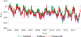
Figure 1 shows a plot of the nearby futures and cash price series at all locations. Prices begin to rise around 2010 and appear to stabilize at a higher level toward the end of the sample period. Figure 2 shows the nearby basis series at all locations. The basis series look much more stable than the spot price series, but around the beginning of 2012, basis does appear to have a lower mean value compared with the preceding years. Figure 3 shows plots of the September basis series, which is quite similar to the nearby series with a somewhat more marked decline over the sample period.
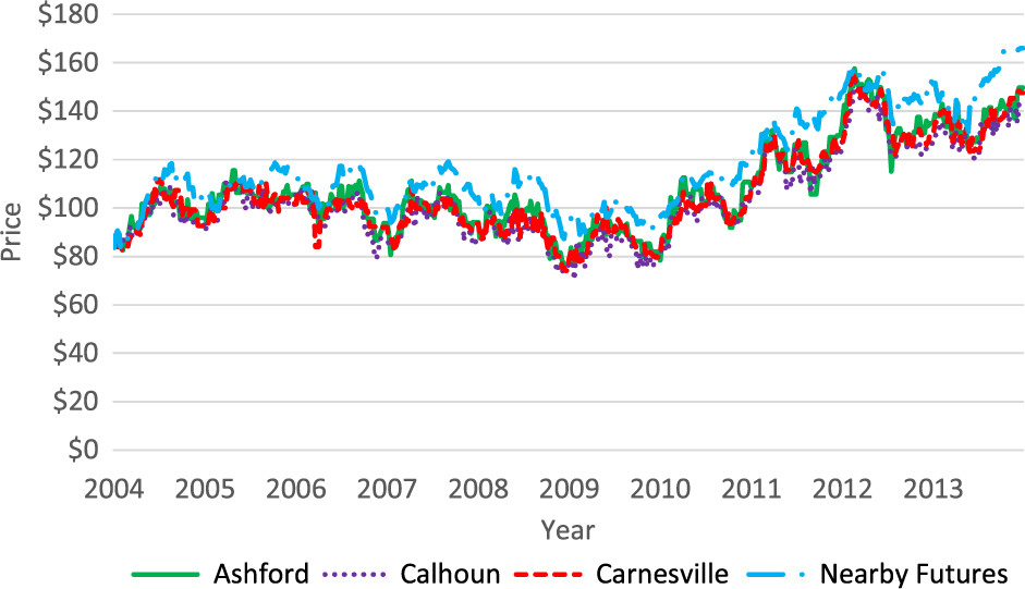
Figure 1. Feeder cattle nearby futures and spot prices at three Georgia locations, 2004–2013.
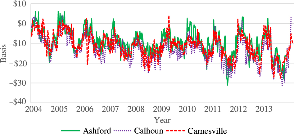
Figure 2. Nearby feeder cattle basis at three Georgia locations, 2004–2013.
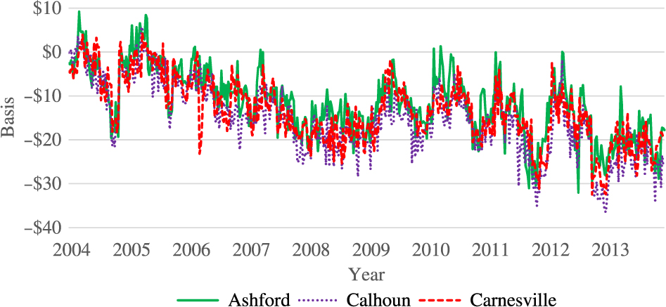
Figure 3. September feeder cattle basis at three Georgia locations, 2004–2013.
Table 1 presents summary statistics for the time series examined in this study. Average nearby basis varies between −$9.41 and –$13.06 per hundredweight while September basis varies between −$11.80 and −$15.45 per hundredweight. All basis series sometimes take positive values; however, as the mean suggests, they are typically negative. September basis has a slightly higher (around $1 per hundredweight) standard deviation than nearby basis. Diesel prices stayed around $3 per gallon throughout the period. Corn prices varied substantially, with a minimum value of $1.87 and a maximum value of $8.34 per bushel.
Table 1. Summary statistics

4.1. Unit root and structural break tests
All series are tested for stationarity using the Bayesian unit root test developed by Dorfman (Reference Dorfman1995), which is based on an autoregressive time series model.Footnote 4 The results are presented in Table 2. The posterior probabilities of stationarity are quite high for both nearby and September basis series at all locations. The probability of stationarity is not as high for corn and diesel prices, but it is still around 75%. In the presence of a unit root, a typical transformation is the first differencing. However, the interpretation of first-differenced variables might be difficult. Therefore, even though somewhat arbitrary, we take the slightly lower, but still well above 50% probabilities of stationarity for corn and diesel to still indicate the lack of a unit root, and, thus, use the prices of corn and diesel in levels.Footnote 5
Table 2. Posterior probabilities of stationarity

Given the great deal of upheaval in financial markets during the sample period and evidence that basis may be getting harder to predict, all six basis series are also examined for structural breaks using the Bayesian test developed by Barry and Hartigan (Reference Barry and Hartigan1993). This procedure tests for a structural break directly in a given time series as opposed to analyzing changes in coefficient estimates in a regression model.Footnote 6 The results, in the form of posterior probabilities of a structural break, are presented in Figure 4. The test indicates structural breaks in 2006 and 2012.Footnote 7 The 2012 break might be attributable to the severe drought around this time. These structural breaks do not affect the sample period (2004–2011) that can be used to create the naïve, historic moving average basis forecasts in models (1) and (2) as they do not require estimation of parameters. However, because structural breaks will result in inconsistent parameter estimates, the years 2009–2010 are used as the in-sample period for regressions to estimate model parameters in equations (3) to (10), and the year 2011 is reserved for out-of-sample forecast evaluation. Because the data frequency is weekly, this creates a total of 104 in-sample observations to estimate model parameters and 52 observations to evaluate out-of-sample forecast performance.
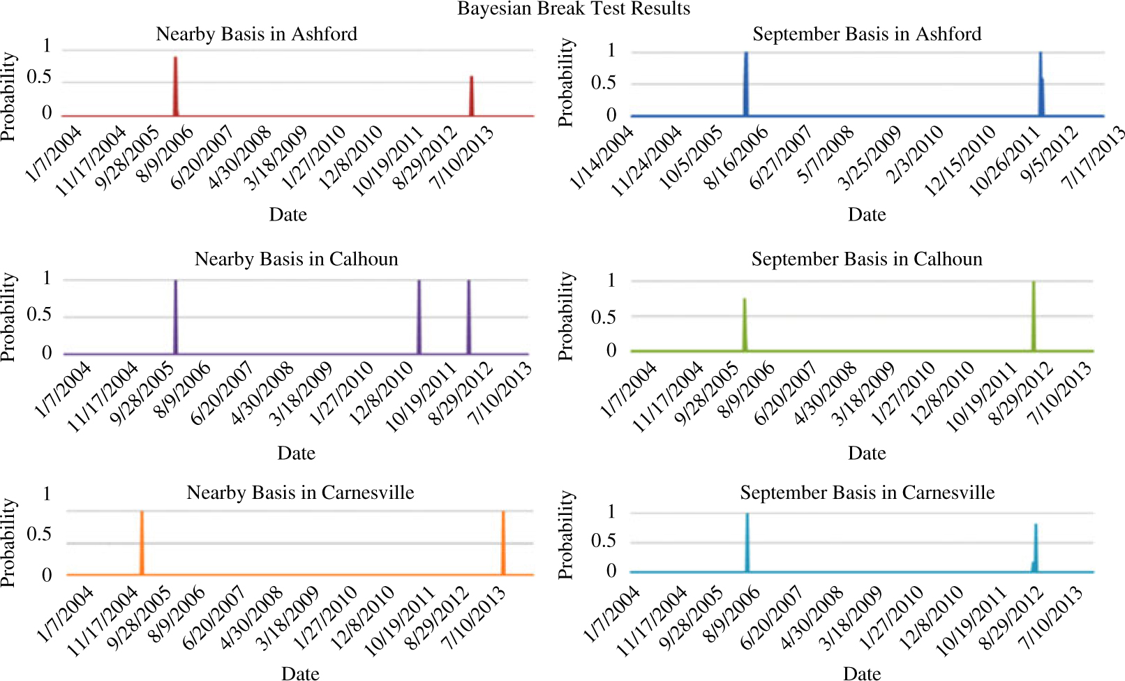
Figure 4. Posterior probabilities of a structural break in feeder cattle basis, 2004–2013.
5. Results
For the one-step ahead forecasts,Footnote 8 a total of 34 models are considered. Because the HMA and YAR models contain yearly autoregressive lags as their sole explanatory variables, these are not included among the models for the four- and eight-step ahead forecasts, resulting in a total of 25 models for these forecasts horizons. Results for the basis forecasts are presented in Tables 3 and 4. Each table presents the five best performing regression models ranked by their out-of-sample root mean squared error (RMSE)Footnote 9 and provides those five models’ estimated posterior model probabilities within the BMA framework.Footnote 10 The tables also present the performances of the BMA model, the best performing naïve model, and the model with the highest posterior model probability. It should be noted that posterior model probability is not a measure to evaluate forecasting performance. It represents the weight the data assign to a given model among the alternative models. Thus, although a higher posterior model probability indicates that the model fits to the in-sample observations better compared with models with lower posterior model probabilities, it does not provide a measure of their fit to out-of-sample observations.
5.1. Nearby basis forecasts
Out-of-sample forecast performance measures for the nearby basis models are presented in Table 3. For the one-step-ahead forecast, a weekly autoregressive model of variable length, given in equations (7) and (8), performs better at all locations compared with other regression models considered. The inclusion of fundamental variables improves these models’ forecast performance inconsistently across locations, but where it does, the improvement is sometimes fairly large compared with a model without fundamental variables. The BMA model does not outperform the best regression model or the best naïve model. Its RMSE is in the same ballpark as the regression models and the naïve models at the Carnesville location, but at the two other locations examined, the BMA performs worse than the top performing models. Interestingly, the BMA does perform better than the model with the highest posterior probability at all locations. The best naïve model is the no-change model for this short-horizon forecast at all locations. For this forecast horizon, the best performing regression model outperforms the best naïve model as well as the BMA at all locations. The models with the highest posterior probabilities are an AR(3)+ or a YAR(4)+ model. The AR(2)+ and AR(3)+ perform in the top five models as ranked by RMSE, but the YAR(4)+ does not perform particularly well for this forecast horizon at any location.
Table 3. Nearby basis forecast results

Notes: AR, weekly autoregressive (equations 7–8); BMA, Bayesian model averaging; CMI, current market information (equations 9–10); HMA, historical moving average regressions (equations 3–4); naïve, last observed (equation 1) or historical moving average (equation 2); M, number of models in the BMA; Post Prob, posterior model probability; RMSE, root mean squared error; YAR, yearly autoregressive (equations 5–6). Plus sign (+) indicates inclusion of fundamental variables.
For the 4-week-ahead forecasts, the best performing regression model varies substantially across locations. Highlighting model uncertainty when forecasting basis, many different types of models perform well within a location as well as across locations. The BMA model produces forecast errors in the ballpark of the top five regression models, and the best naïve model performs inconsistently compared with the regression and BMA models. The best naïve is still a no-change model at one location (Calhoun), whereas a 4-year average performs best at the other two locations (Carnesville and Ashford). Although not presented in the table, the difference between a no-change model and a 3- or 4-year average is quite small for this forecast horizon. It is interesting that at this forecast horizon the model with the highest posterior model probability appears in the top five only for one location, even though the BMA model performs comparably with these models. Unlike in the 1-week-ahead forecasts, the BMA model performs almost exactly the same as the model with the highest posterior probability. The model with the highest posterior model probability is the same at each location: a YAR(4)+ model.
For 8-week-ahead forecasts, the best performing regression model outperforms the best naïve model and the BMA model at two locations, while a naïve model continues to perform best at the third location (Carnesville). At this forecast horizon, a 4-year moving average performs best among the naïve models considered. The best performing regression model varies across locations, although the CMI models appear the most frequently among the top performers. At Ashford and Calhoun, the best regression models all contain the fundamental variables, whereas at the Carnesville none of the best performing models contain those fundamental variables. Models with the highest posterior probability do not appear in the top five regression models. The BMA models perform somewhat worse than the top five models at this forecast horizon.
5.2. September basis forecasts
The performance measures of the September basis forecasts are presented in Table 4. At the 1-week-ahead forecast horizon, the weekly autoregressive models perform best. The highest probability model is also an autoregressive model: either an AR(2)+ or AR(3)+. The BMA models perform quite similarly, and at one location (Calhoun), the BMA model actually performs better than any of the regression models. Weekly autoregressive models perform in the top five at all locations, although the specific model and whether additional fundamental variables improve the forecasts differ by location.
Table 4. September basis forecast results

Notes: AR, weekly autoregressive (equations 7–8); BMA, Bayesian model averaging; CMI, current market information (equations 9–10); HMA, historical moving average regressions (equations 3–4); naïve, last observed (equation 1) or historical moving average (equation 2); M, number of models in the BMA; Post Prob, posterior model probability; RMSE, root mean squared error; YAR, yearly autoregressive (equations 5–6). Plus sign (+) indicates inclusion of fundamental variables.
For four-step-ahead September basis forecasts, regression models perform at least as well as the naïve forecast. The BMA model performs noticeably worse than the top five regression models at all locations, possibly because the models with the highest model probability perform relatively poorly compared with the best regression models. The best naïve model also performs poorly at two locations while it performs comparably to the best model at the third location (Carnesville). The same model uncertainty observed in the four-step-ahead nearby basis forecast appears at this forecast horizon too, as many different types of models appear in the top five for the three locations considered.
For the eight-step-ahead September basis forecasts, the best regression models vary across locations as well, but the best models all contain the fundamental explanatory variables. The best performing regression models receive low model probabilities, and the BMA model performs quite poorly at two locations, while at the third (Carnesville) it is comparable to the best models. Again, regression models generally perform better than the naïve forecasts.
6. Conclusions
This study examines feeder cattle basis forecasts at three Georgia locations with the aim of identifying potentially new and better ways to forecast basis. Both nearby basis and basis forecasts for a specific month (September) are examined. This second type of forecast has not previously been examined but would be useful in making decisions on distant future marketing plans. Forecasts are created using a naïve moving average and many regression-based models. The regression models are also used to form a combined forecast using BMA. Models are then evaluated based on their out-of-sample forecast performance.
For both the forecasts made with the nearby basis series and the September basis series, the best performing regression models at a given forecast horizon vary across locations, and as in previous studies on grain and livestock basis, the best model differs by forecast horizon. Autoregressive models do well for the shortest horizon, whereas models with yearly lags or current market information do better for longer-horizon forecasts. Further, the BMA model outperforms the best naïve forecast for longer forecast horizons at two of the three locations selected.
The addition of fundamental variables does not consistently improve the performance of one-step-ahead forecasts. However, most of the best regression models for the longer-horizon forecasts contain the fundamental variables. At all locations and all forecast horizons, the model with the highest posterior model probability assigned by the Bayesian estimation contains the fundamental variables. This suggests that fundamental variables are crucial in explaining basis, and therefore, they should be incorporated in basis forecasting models.
For both the nearby and September basis forecasts, the BMA model and the regression models perform comparably to the best naïve model for the one-step-ahead forecast, but for longer-horizon forecasts, the best regression model produces a lower forecast error than the benchmark naïve, generally around $0.50 to $1 per hundredweight. This improvement in the basis forecast would considerably affect the profit/loss margin from a hedging position at the time the hedge is lifted depending on whether the basis was over- or underestimated when the hedge was started, especially for a large-scale cattle feeder largely relying on basis forecasts while managing price risk through futures contracts. For the shortest forecast horizon, a no-change naïve model performs best. For the longest forecast horizon, a 3- or 4-year moving average performs best among the naïve models considered. For the four-step-ahead forecast, a no-change model and a 3- or 4-year moving average perform quite similarly. The naïve models’ performance generally fell in line with previous studies’ findings with no-change models doing well for the shortest forecasts and 3- or 4-year moving averages doing best for longer forecasts.
The regression models performed similarly or better than the benchmark naïve models at all forecast horizons considered. The BMA model’s performance in forecasting basis varied by location and forecast horizon: in one instance, it performed best; sometimes it performed comparably; and some other times, it performed relatively poorly. However, the set of regression models and explanatory variables included in the BMA process can be extended for further investigation of potential improvements in cattle basis forecasting. The application of this process to agricultural commodities also warrants investigation. The higher frequency of data and the availability of data for more explanatory variables may yield different results.
The disparity in the best performing regression model across locations and over different forecast horizons with both the nearby and September basis series highlights the presence of model uncertainty in using regression models to forecast basis. Though performance of regression models varied substantially, the BMA model always performed comparably regardless of location or forecast horizon when forecasting nearby basis. Although it may not be possible to generalize without further analysis of more locations and commodities, these results suggest that basis forecasts that use regressions should account for model uncertainty. A model that performs well at one location may perform poorly at another, and the best regression model also might change based on forecast horizon. BMA as it is implemented in this article accounts for model uncertainty at the locations and for the commodities considered. The BMA model typically performs better than the model with the highest model probability. Although the BMA model’s performance is not always outstanding compared with individual regression models and the naïve forecast, the BMA model was among the top 10 models seven times out of nine cases for nearby basis forecasts, and four times for September basis forecast. This demonstrates that examining many different models as potential forecast candidates may be warranted to identify a good model.


 Open access