


1 Introduction
Interfaces between fluids appear throughout science, technology, industry and nature. Bubbles are generated by crashing waves in the ocean, by agitation in washing machines, during froth flotation in the mining and energy industries and when super-saturated, dissolved gasses nucleate and grow bubbles in sodas, geysers, canned whipped cream and during fermentations. Droplets of one liquid may be emulsified in a second immiscible liquid – as found in foods, consumer products, pharmaceuticals, oil production and processing. Sea surfaces may be smooth and glassy, or riddled with capillary waves.
Almost without exception, ‘surface-active’ molecules and/or particles – collectively called ‘surfactants’ – control the initiation, dynamics and behaviour of these and other processes. The fluid mechanics community knows quite well that surfactants reduce the interfacial tension of liquid surfaces, thus lowering the energetic cost of blowing bubbles or inflating lungs. By extension, surfactant gradients are well known to exert ‘Marangoni’ stresses on fluid interfaces, often driving or influencing the flow of the fluids that form them.
Surfactants also impact a variety of scientific and industrial processes through a number of processes and mechanisms that are not so clear. A simple example highlights the difficulties that arise: the buoyant rise of a small bubble through a Newtonian liquid (figure 1). A bubble of radius $R$
with a perfectly clean surface rises according to the classic Stokes drag calculation, imposing a no-shear stress boundary condition, to give
$R$
with a perfectly clean surface rises according to the classic Stokes drag calculation, imposing a no-shear stress boundary condition, to give
 $$\begin{eqnarray}U^{c}=\frac{F}{4\unicode[STIX]{x03C0}\unicode[STIX]{x1D702}R},\end{eqnarray}$$
where $F$
is the drag and
$F$
is the drag and $\unicode[STIX]{x1D702}$
is the shear viscosity of the fluid. In many cases, however, bubbles rise with velocities much closer to
$\unicode[STIX]{x1D702}$
is the shear viscosity of the fluid. In many cases, however, bubbles rise with velocities much closer to
 $$\begin{eqnarray}U^{s}=\frac{F}{6\unicode[STIX]{x03C0}\unicode[STIX]{x1D702}R},\end{eqnarray}$$
as one would expect for a rigid particle. What is the reason?
A vague acknowledgment that surfactants exist does not help much. In fact, a number of phenomena may be responsible for the slower rise. Boussinesq (Reference Boussinesq1913) originally surmised that the fluid/gas interface might itself have some surface-excess viscosity, dissipating energy as it deforms (figure 1 b). A more modern understanding holds that such surface viscosities are established by the surfactants adsorbed to the interface. Even without surface rheology, bulk viscous stresses advect surfactant to the rear of the bubble as it rises (figure 1 e), establishing a concentration gradient that drives a counter-acting Marangoni stress (figure 1 f). The strength of this gradient depends on how the surfactant responds (Levich Reference Levich1962) to being driven out of equilibrium. Insoluble surfactants diffusively fight to equalize their surface concentration (figure 1 g). Soluble surfactants adsorb and desorb from the interface to maintain an equilibrium (figure 1 h). If this equilibration process occurs slowly, gradients (and Marangoni stresses) are strong; conversely, rapid equilibration causes only weak gradients.

Figure 1. (a) ‘Hidden’ surfactant variables modify the interfacial flow of a rising bubble such that it might behave like a clean drop, a rigid particle or somewhere in between. The associated surfactant transport processes are not often easy to differentiate, and systems may exhibit one or a non-trivial combination of several processes. (b–d) For instance, an interfacial or surface excess viscosity can resist the surface flow. The solid lines depict surface flow, and dashed red arrows indicate tangential (viscous) stresses resisting deformation. (e–g) Alternatively, surfactants swept to the rear of the bubble build a concentration gradient and generate a counter-acting Marangoni stress (dashed red arrows) that resists surface convection (blue arrows). These Marangoni forces may be weakened by surface diffusion against the gradient. (h–j) If the surfactant is soluble, adsorption/desorption from the bulk can drive the surface concentration back to equilibrium over a finite time. This process might be controlled by (i) diffusive transport in the bulk across bulk concentration gradients over a time scale $\unicode[STIX]{x1D70F}_{d}$
, or by (j) the finite-rate kinetics over a finite time scale
$\unicode[STIX]{x1D70F}_{d}$
, or by (j) the finite-rate kinetics over a finite time scale $\unicode[STIX]{x1D70F}_{k}$
.
$\unicode[STIX]{x1D70F}_{k}$
.
It is hard to imagine a simpler experiment than this – measuring the rise velocity of a nearly spherical bubble in a liquid, say as a function of bubble radius. If the measured velocity matches $U^{c}$
from (1.1), one can conclude that the drop is clean. If, on the other hand, the measured velocity is slower than
$U^{c}$
from (1.1), one can conclude that the drop is clean. If, on the other hand, the measured velocity is slower than $U^{c}$
, the discrepancy might be caused by (a) inherent surface viscosity; (b) surface viscosity due to a surfactant; (c) flow-induced Marangoni stresses from an insoluble surfactant; (d) flow-induced Marangoni stresses from a soluble surfactant, the magnitude of which might be determined by (i) adsorption/desorption rate kinetics; or (ii) surfactant diffusion across the bubble; (iii) convection–diffusion transport of surfactant across the bubble. However sensible figure 1(a) may seem, the
$U^{c}$
, the discrepancy might be caused by (a) inherent surface viscosity; (b) surface viscosity due to a surfactant; (c) flow-induced Marangoni stresses from an insoluble surfactant; (d) flow-induced Marangoni stresses from a soluble surfactant, the magnitude of which might be determined by (i) adsorption/desorption rate kinetics; or (ii) surfactant diffusion across the bubble; (iii) convection–diffusion transport of surfactant across the bubble. However sensible figure 1(a) may seem, the $x$
-axis is often difficult to unambiguously determine.
$x$
-axis is often difficult to unambiguously determine.
This difficulty – of identifying mechanisms by which surfactants act – arises much more broadly, in systems and processes that are much more complicated. Surfactants influence film thicknesses in coating flows (Quéré Reference Quéré1999; Shen et al. Reference Shen, Gleason, McKinley and Stone2002; Scheid et al. Reference Scheid, Delacotte, Dollet, Rio, Restagno, van Nierop, Cantat, Langevin and Stone2010), the dispersion of surface waves (Levich Reference Levich1962; Lucassen & Hansen Reference Lucassen and Hansen1966), the dynamics and thicknesses of spreading films (Troian, Herbolzheimer & Safran Reference Troian, Herbolzheimer and Safran1990; Darhuber & Troian Reference Darhuber and Troian2005) and the lifetime of foams and emulsions (Langevin Reference Langevin2000; Cohen-Addad, Höhler & Pitois Reference Cohen-Addad, Höhler and Pitois2013). Mechanisms by which these effects arise can be complicated and varied. For example, surfactants may provide additional energetic barriers to droplet and bubble coalescence: surfactants on either side of a liquid film may repel each other sterically or electrostatically, and thus retard or arrest the thinning of the film (Bibette et al. Reference Bibette, Morse, Witten and Weitz1992; Stancik, Kouhkan & Fuller Reference Stancik, Kouhkan and Fuller2004). Alternatively, or additionally, dynamic mechanisms may also act: surfactants advected by thinning films establish gradients, and thus Marangoni stresses, that oppose the film drainage (Leal Reference Leal2004). Monolayers of surfactant may introduce an excess surface viscosity, elasticity or visco-elasticity that retards or alters film thinning (Langevin Reference Langevin2000). Even more subtle, surfactant exchange between the bulk and the interface can mimic surface-excess (dilatational) viscosity, masking the physical origin of the dissipation (Levich Reference Levich1962; Lucassen & van den Tempel Reference Lucassen and van den Tempel1972).
Despite the controlling influence that surfactants exert over many fluid systems, the surfactants themselves are effectively invisible in most experiments, and to most techniques. Interpreting such experiments becomes challenging at best, given that physically distinct surfactant processes impact measurements in identical ways. In many ways, surfactants behave like ‘hidden variables’ that cannot be measured directly, yet influence fluid flows so profoundly that they must be determined in order to understand even gross, qualitative fluid phenomena. Surfactant distributions are thus typically inferred from observable fluid phenomena – e.g. measured fluid velocity fields, free surface dynamics or Laplace pressure measurements. Connecting measurements and observations with the underlying surfactant fields, however, requires some model for the dynamics and mechanics of surfactant transport.
The fact that physically distinct surfactant processes can impact measurable properties in the same way – while the surfactants themselves elude detection – has caused significant confusion. For example, the origin and even existence of surface rheology has long been controversial (Scriven & Sternling Reference Scriven and Sternling1960), with justifiable reason: if Marangoni stresses can explain an experimental observation, what is the need to invoke surface rheology? Why should a rightly sceptical scientist invoke some nebulous phenomenon, when established processes can explain measurements? At the same time, plausible mechanisms should not be dismissed out of hand: after all, however familiar a process may be, it might actually not be the one responsible for an observation.
Understanding these surfactant systems – and ultimately predicting and designing them – requires that these mechanisms and processes be differentiated unambiguously. This might be accomplished by specifically designing experiments to excite one process but not others: forcing a surfactant-laden interface to deform in a purely shear fashion – i.e. with zero compression or dilation – should not trigger Marangoni stresses, but would be sensitive to surface shear rheology. In systems with compression, it may not be easy or even possible to separate stresses cause by surface dilatational viscosity – an intrinsic material property – from an effective surface viscoelasticity due to surfactant adsorption and desorption, surface and bulk diffusion, aggregation or phase transitions, Marangoni flows, or some combination of these processes. Knowing how these processes scale with e.g. system geometry, fluid velocity, surfactant concentrations and properties, however, might suggest complementary experiments to tease apart these influences.
The objective of this Perspective, then, is to enumerate and elucidate the multitude of transport processes involved in the formation, flow and rheological response of surfactant-laden interfaces, and therefore to better understand, interpret, predict and design surfactant/fluid flows and materials. By presenting these diverse phenomena in one comprehensive piece, described using the same language and within the same context, we hope to to empower the fluid mechanics and soft condensed matter physics communities to discern and differentiate between the various dynamics surfactants might cause. We also hope to connect the fluid mechanics community to the physical chemistry literature on surfactants, which is more steeped in equilibrium thermodynamics than typical fluid mechanicians have at their fingertips. To this end, this perspective highlights paradigmatic examples chosen for their paedagogic value in weaving a coherent and compelling picture of surfactant dynamics, rather than a comprehensive treatment of this vast literature.
In what follows, we treat surfactants from the physical–chemical standpoint, hopefully giving the fluid mechanician enough basis to connect with the surfactant literature. We will start with equilibrium arguments about surface tension and surface pressure, including the equilibrium properties of soluble and insoluble surfactants (§ 2). We then move on to dynamic processes – which tend to be more familiar to the fluid mechanician – and discuss the various ways in which surfactant is transported (§ 3). We will touch on surface rheology, which is relatively unfamiliar to both communities. Then, in § 4, we show how even these most basic treatments give rise to remarkable richness in a series of paradigmatic problems: (§ 4.1) the buoyant translation of bubbles and drops; (§ 4.2) the oscillatory compression of soluble monolayers; (§ 4.3) surface wave dynamics; (§ 4.4) coating flows; (§ 4.5) foam drainage; and (§ 4.6) particle motion within surfactant-laden interfaces. These problems are chosen both for their ubiquity and importance, as well as the non-trivial and rich phenomena that appear even for the simplest assumptions for the processes described in § 3. Finally, in § 5, we present a variety of complexities that arise even in common surfactant systems – beyond the ‘simplest’ treatments in §§ 2–4 – with the goal of highlighting areas where standard assumptions may not capture experimental observations, and to encourage new directions for research and innovation.
2 Interfaces at equilibrium
2.1 Surface tension and its origins
Surface tension originates from the imbalance in mutually attractive forces felt by molecules near an interface. A liquid molecule in the bulk of a fluid is surrounded by neighbours of the same kind, all exerting attractive intermolecular forces. Molecules that are surrounded experience no net force, due to the symmetric distribution of their neighbours. A force is required to pull one molecule out of the bulk liquid, however, one must supply enough free energy to break the $N$
‘bonds’, each of strength
$N$
‘bonds’, each of strength $\unicode[STIX]{x0394}U$
.
$\unicode[STIX]{x0394}U$
.
A molecule near an immiscible fluid–fluid interface, however, feels a net force towards the fluid phase with higher intermolecular attractions. These interfacial molecules are in an energetically unfavourable state, and creation of additional interfacial area is expensive. A fluid system, therefore, minimizes interfacial area. The surface tension $\unicode[STIX]{x1D6FE}$
of a fluid–fluid interface is then the energy associated with creating excess area, which depends on the strength of intermolecular forces in both bulk phases. For example, a clean air–water interface has
$\unicode[STIX]{x1D6FE}$
of a fluid–fluid interface is then the energy associated with creating excess area, which depends on the strength of intermolecular forces in both bulk phases. For example, a clean air–water interface has $\unicode[STIX]{x1D6FE}\approx 0.072~\text{J}~\text{m}^{-2}$
, or equivalently,
$\unicode[STIX]{x1D6FE}\approx 0.072~\text{J}~\text{m}^{-2}$
, or equivalently, $72~\text{mN}~\text{m}^{-1}$
.
$72~\text{mN}~\text{m}^{-1}$
.
The surface tension of a liquid can be estimated with the simple thought experiment depicted in figure 2. Each molecule in the bulk liquid has attractive interactions with $N$
neighbours. Cleaving the bulk into two, and therefore creating two interfaces, requires
$N$
neighbours. Cleaving the bulk into two, and therefore creating two interfaces, requires $N/2$
bonds, each of energy
$N/2$
bonds, each of energy $\unicode[STIX]{x0394}U$
, to be supplied for every interfacial molecule. Given
$\unicode[STIX]{x0394}U$
, to be supplied for every interfacial molecule. Given $\unicode[STIX]{x1D6E4}_{s}$
molecules per unit area, cleaving these bonds requires an energy per unit area,
$\unicode[STIX]{x1D6E4}_{s}$
molecules per unit area, cleaving these bonds requires an energy per unit area, $\unicode[STIX]{x1D6FE}$
, given by
$\unicode[STIX]{x1D6FE}$
, given by
 $$\begin{eqnarray}\unicode[STIX]{x1D6FE}\sim N\unicode[STIX]{x0394}U\unicode[STIX]{x1D6E4}_{s}.\end{eqnarray}$$
Of course, molecules at the interface might relax and re-arrange, changing the energetics of interfacial molecules, but we neglect these small changes. The interaction energy $N\unicode[STIX]{x0394}U$
must be
$N\unicode[STIX]{x0394}U$
must be $O(k_{B}T)$
in order for the bulk to be a liquid: if the interaction energy were much stronger than thermal energy (
$O(k_{B}T)$
in order for the bulk to be a liquid: if the interaction energy were much stronger than thermal energy ( $N\unicode[STIX]{x0394}U\gg k_{B}T$
), molecules would lock in place as a solid or glass, whereas if it were much weaker (
$N\unicode[STIX]{x0394}U\gg k_{B}T$
), molecules would lock in place as a solid or glass, whereas if it were much weaker ( $N\unicode[STIX]{x0394}U\ll k_{B}T$
), the molecules would fly apart to form a gas. Ignoring numerical prefactors, this suggests a surface tension
$N\unicode[STIX]{x0394}U\ll k_{B}T$
), the molecules would fly apart to form a gas. Ignoring numerical prefactors, this suggests a surface tension
 $$\begin{eqnarray}\unicode[STIX]{x1D6FE}\sim k_{B}T\unicode[STIX]{x1D6E4}_{s}.\end{eqnarray}$$
However crude, this approximation gives reasonable estimates: assuming water molecules to have an approximate radius $r_{w}\sim 0.2~\text{nm}$
(based on the bulk density and molecular mass of water) suggests water molecules occupy the interface with density
$r_{w}\sim 0.2~\text{nm}$
(based on the bulk density and molecular mass of water) suggests water molecules occupy the interface with density $\unicode[STIX]{x1D6E4}_{s}\sim 9~\text{nm}^{-2}$
. Using
$\unicode[STIX]{x1D6E4}_{s}\sim 9~\text{nm}^{-2}$
. Using $k_{B}T\sim 4~\text{pN}~\text{nm}$
at room temperature gives
$k_{B}T\sim 4~\text{pN}~\text{nm}$
at room temperature gives $\unicode[STIX]{x1D6FE}\sim 40~\text{mN}~\text{m}^{-1}$
, which is within a factor of two of the measured value
$\unicode[STIX]{x1D6FE}\sim 40~\text{mN}~\text{m}^{-1}$
, which is within a factor of two of the measured value $72~\text{mN}~\text{m}^{-1}$
. More generally, most liquids with approximately Angstrom radii thus have surface tensions in the tens of
$72~\text{mN}~\text{m}^{-1}$
. More generally, most liquids with approximately Angstrom radii thus have surface tensions in the tens of $\text{mN}~\text{m}^{-1}$
.
$\text{mN}~\text{m}^{-1}$
.

Figure 2. A liquid molecule in the bulk of a fluid experiences no net force due to a (time-averaged) symmetric distribution of neighbours. Creating an interface, however, requires breaking intermolecular ‘bonds’ on the interface and is energetically expensive.
Surface tension can be alternatively interpreted in terms of the mechanical work done in stretching an interface. If the application of a force $F$
within the plane of the interface changes its area by
$F$
within the plane of the interface changes its area by $\text{d}A$
, the net change in energy is a sum of mechanical work done and the surface energy associated with surface tension
$\text{d}A$
, the net change in energy is a sum of mechanical work done and the surface energy associated with surface tension
 $$\begin{eqnarray}\text{d}U=-F\,\text{d}x+\unicode[STIX]{x1D6FE}\,\text{d}A.\end{eqnarray}$$
At mechanical equilibrium, $\text{d}U=0$
, and writing
$\text{d}U=0$
, and writing $\text{d}A=\ell \,\text{d}x$
where
$\text{d}A=\ell \,\text{d}x$
where $\ell$
is the width of the interfacial layer, we find
$\ell$
is the width of the interfacial layer, we find $\unicode[STIX]{x1D6FE}=F/\ell$
. In other words, surface tension gives the force per unit length to create interfacial area.
$\unicode[STIX]{x1D6FE}=F/\ell$
. In other words, surface tension gives the force per unit length to create interfacial area.
Finally, $\unicode[STIX]{x1D6FE}$
can be thought of as a surface stress, pulling isotropically within the plane of the interface, and is therefore analogous to a negative three-dimensional (3-D) pressure. We will soon extend this analogy with 3-D pressure, as surfactants exert a ‘surface pressure’,
$\unicode[STIX]{x1D6FE}$
can be thought of as a surface stress, pulling isotropically within the plane of the interface, and is therefore analogous to a negative three-dimensional (3-D) pressure. We will soon extend this analogy with 3-D pressure, as surfactants exert a ‘surface pressure’, $\unicode[STIX]{x1D6F1}$
, against the surface tension
$\unicode[STIX]{x1D6F1}$
, against the surface tension $\unicode[STIX]{x1D6FE}$
of the clean interface.
$\unicode[STIX]{x1D6FE}$
of the clean interface.
Unlike bulk 3-D fluids, however, surfaces are two-dimensional and can be curved, which modifies the static stress required to create additional area. For example, increasing the volume of a bubble of gas $A$
suspended at equilibrium in liquid
$A$
suspended at equilibrium in liquid $B$
increases the surface area of the bubble, and therefore its interfacial energy. If the bubble radius increases from
$B$
increases the surface area of the bubble, and therefore its interfacial energy. If the bubble radius increases from $R$
to
$R$
to $R+\text{d}R$
, the net free energy change is
$R+\text{d}R$
, the net free energy change is
 $$\begin{eqnarray}\text{d}U=-p_{A}\,\text{d}V_{A}-p_{B}\,\text{d}V_{B}+\unicode[STIX]{x1D6FE}_{AB}\,\text{d}A,\end{eqnarray}$$
where $\unicode[STIX]{x1D6FE}_{AB}$
is the surface tension of the
$\unicode[STIX]{x1D6FE}_{AB}$
is the surface tension of the $A$
–
$A$
– $B$
interface,
$B$
interface, $p_{A}$
and
$p_{A}$
and $p_{B}$
are the pressures inside and outside the bubble, respectively,
$p_{B}$
are the pressures inside and outside the bubble, respectively, $\text{d}V_{A}=-\text{d}V_{B}=4\unicode[STIX]{x03C0}R^{2}\,\text{d}R$
and
$\text{d}V_{A}=-\text{d}V_{B}=4\unicode[STIX]{x03C0}R^{2}\,\text{d}R$
and $\text{d}A=8\unicode[STIX]{x03C0}R\,\text{d}R$
. Imposing
$\text{d}A=8\unicode[STIX]{x03C0}R\,\text{d}R$
. Imposing $\text{d}U=0$
to satisfy mechanical equilibrium reveals the well-known Laplace pressure jump across the bubble surface:
$\text{d}U=0$
to satisfy mechanical equilibrium reveals the well-known Laplace pressure jump across the bubble surface:
 $$\begin{eqnarray}\unicode[STIX]{x0394}p=p_{A}-p_{B}=\frac{2\unicode[STIX]{x1D6FE}_{AB}}{R}.\end{eqnarray}$$
The larger the interfacial curvature or surface tension, the greater is the bulk fluid pressure required to maintain the system in equilibrium: smaller bubbles have a higher internal pressure. More generally, the Laplace pressure is given by the Young–Laplace equation (Leal Reference Leal2007)
 $$\begin{eqnarray}\unicode[STIX]{x0394}p=\unicode[STIX]{x1D6FE}_{AB}\unicode[STIX]{x1D735}_{s}\boldsymbol{\cdot }\boldsymbol{n},\end{eqnarray}$$
where $\boldsymbol{n}$
is the normal to the interface, pointing away from the fluid
$\boldsymbol{n}$
is the normal to the interface, pointing away from the fluid $A$
,
$A$
, $\unicode[STIX]{x1D735}_{s}=(\unicode[STIX]{x1D644}-\boldsymbol{n}\boldsymbol{n})\boldsymbol{\cdot }\unicode[STIX]{x1D735}$
is the surface gradient operator, and
$\unicode[STIX]{x1D735}_{s}=(\unicode[STIX]{x1D644}-\boldsymbol{n}\boldsymbol{n})\boldsymbol{\cdot }\unicode[STIX]{x1D735}$
is the surface gradient operator, and $\unicode[STIX]{x1D735}_{s}\boldsymbol{\cdot }\boldsymbol{n}$
is the mean curvature of the surface.
$\unicode[STIX]{x1D735}_{s}\boldsymbol{\cdot }\boldsymbol{n}$
is the mean curvature of the surface.
2.2 ‘Dirty’ interfaces: surfactants of different classes
Many surfactants are ‘amphiphilic’ – having both hydrophilic and hydrophobic parts – and adsorb to surfaces to minimize energetically unfavourable interactions. For instance, amphiphilic molecules adsorb to a water–air interface with their hydrophobic tails directed out of the water phase (figure 3). Adsorption to a surface comes at a cost, however: the bulk fluid offers a wider range of translational and rotational micro-states and therefore, a larger entropy per surfactant molecule. At equilibrium, the balance between adsorbed surfactants, with surface concentration $\unicode[STIX]{x1D6E4}$
, and dissolved surfactants, with bulk concentration
$\unicode[STIX]{x1D6E4}$
, and dissolved surfactants, with bulk concentration $C$
, reflects a balance between the (favourable) enthalpy change and the (unfavourable) entropy loss that occurs during adsorption. With increasing bulk concentration, the balance between the energetic expense of hydrophobic groups remaining within the bulk and the entropic loss of moving to the interface tilts in favour of adsorption (figure 3
b,c) and a monolayer of increasing surface concentration
$C$
, reflects a balance between the (favourable) enthalpy change and the (unfavourable) entropy loss that occurs during adsorption. With increasing bulk concentration, the balance between the energetic expense of hydrophobic groups remaining within the bulk and the entropic loss of moving to the interface tilts in favour of adsorption (figure 3
b,c) and a monolayer of increasing surface concentration $\unicode[STIX]{x1D6E4}$
forms at the interface.
$\unicode[STIX]{x1D6E4}$
forms at the interface.

Figure 3. (a) Schematic representation of an amphiphilic molecule. (b,c) Surfactant molecules adsorb to the interface to an extent determined by the competition between (loss of) entropy and energetically favourable interactions during adsorption. Also shown in (c) are the concentration profiles of surfactant (solid line) and water (dashed line) molecules. The ‘excess’ surface concentration is in grey, which represents the amount of surfactant in excess of a hypothetical state where the concentration of dissolved surfactant is constant up until the surface.
The affinity of surfactant molecules towards interfaces creates a surface ‘excess’ concentration, $\unicode[STIX]{x1D6E4}$
. In other words,
$\unicode[STIX]{x1D6E4}$
. In other words, $\unicode[STIX]{x1D6E4}$
is the number of molecules per unit interfacial area in excess of a hypothetical reference state, in which the adjoining bulk phases maintain their constant concentrations (figure 3
c) up until the surface. The position of the surface itself is arbitrary, and is typically chosen such that the surface-excess concentration of the solvent is zero.
$\unicode[STIX]{x1D6E4}$
is the number of molecules per unit interfacial area in excess of a hypothetical reference state, in which the adjoining bulk phases maintain their constant concentrations (figure 3
c) up until the surface. The position of the surface itself is arbitrary, and is typically chosen such that the surface-excess concentration of the solvent is zero.
It is conceptually simple to appreciate the surface-active nature of molecules with physically distinct hydrophilic and hydrophobic portions, as depicted in figure 3(a). Such clearly differentiated portions, however, are not necessary for surface activity. The basic surfactant argument holds just as well for chemically homogeneous molecules or particles that possess an intermediate wettability with respect to the fluids on either side of the interface (Binks Reference Binks2002).
Any species (molecular or particulate) that has a positive surface excess is – by definition – a surfactant. And so – what are the options? How much do they reduce surface tension? What time scales emerge? The equilibrium properties of different classes of surfactants can differ substantially, as shown in figure 4. All cases depict a spherical liquid drop of surface area $A_{i}$
whose shape is deformed and held at a final surface area
$A_{i}$
whose shape is deformed and held at a final surface area $A_{f}$
, for an increase of
$A_{f}$
, for an increase of $\unicode[STIX]{x0394}A$
. The clean, surfactant-free drop (figure 4
a) serves as a base case: the extra surface area
$\unicode[STIX]{x0394}A$
. The clean, surfactant-free drop (figure 4
a) serves as a base case: the extra surface area $\unicode[STIX]{x0394}A$
created by deforming at the interface comes at the cost of the ‘clean’ surface tension
$\unicode[STIX]{x0394}A$
created by deforming at the interface comes at the cost of the ‘clean’ surface tension $\unicode[STIX]{x1D6FE}_{0}$
of the liquid/liquid interface, requiring an additional energy
$\unicode[STIX]{x1D6FE}_{0}$
of the liquid/liquid interface, requiring an additional energy $\unicode[STIX]{x0394}U=\unicode[STIX]{x1D6FE}_{0}\unicode[STIX]{x0394}A$
.
$\unicode[STIX]{x0394}U=\unicode[STIX]{x1D6FE}_{0}\unicode[STIX]{x0394}A$
.

Figure 4. Examples of change in surface energy upon deformation of a drop with surface-active molecules or particles.
Many surfactants are soluble, meaning that the surface excess concentration $\unicode[STIX]{x1D6E4}$
of adsorbed surfactant equilibrates with the dissolved concentration
$\unicode[STIX]{x1D6E4}$
of adsorbed surfactant equilibrates with the dissolved concentration $C$
according to an isotherm (table 1). When a drop is initially coated with soluble surfactant at surface coverage
$C$
according to an isotherm (table 1). When a drop is initially coated with soluble surfactant at surface coverage $\unicode[STIX]{x1D6E4}_{eq}$
and then deformed to create extra area
$\unicode[STIX]{x1D6E4}_{eq}$
and then deformed to create extra area $\unicode[STIX]{x0394}A$
, the interfacial concentration
$\unicode[STIX]{x0394}A$
, the interfacial concentration $\unicode[STIX]{x1D6E4}$
drops below its equilibrium with the bulk concentration
$\unicode[STIX]{x1D6E4}$
drops below its equilibrium with the bulk concentration $C$
. Bulk surfactant is then driven to adsorb to the interface, until the equilibrium surface coverage (
$C$
. Bulk surfactant is then driven to adsorb to the interface, until the equilibrium surface coverage ( $\unicode[STIX]{x1D6E4}_{f}=\unicode[STIX]{x1D6E4}_{eq}$
) is restored (figure 4
b). At steady state, the surface tension of the drop is thus equal to the initial, equilibrium value
$\unicode[STIX]{x1D6E4}_{f}=\unicode[STIX]{x1D6E4}_{eq}$
) is restored (figure 4
b). At steady state, the surface tension of the drop is thus equal to the initial, equilibrium value $\unicode[STIX]{x1D6FE}_{eq}(C)$
, which is lower than the clean surface tension
$\unicode[STIX]{x1D6FE}_{eq}(C)$
, which is lower than the clean surface tension $\unicode[STIX]{x1D6FE}_{0}$
. The energetic cost of this deformation is thus reduced to
$\unicode[STIX]{x1D6FE}_{0}$
. The energetic cost of this deformation is thus reduced to $\unicode[STIX]{x0394}U=\unicode[STIX]{x1D6FE}_{eq}\unicode[STIX]{x0394}A$
.
$\unicode[STIX]{x0394}U=\unicode[STIX]{x1D6FE}_{eq}\unicode[STIX]{x0394}A$
.
Some surfactants are insoluble in the bulk solution, meaning that there are no surfactants dissolved in the ‘reservoir’, and the number $N$
of surfactants on an interface remains constant. Deforming a drop coated with insoluble surfactants (figure 4
c) decreases the surface concentration to
$N$
of surfactants on an interface remains constant. Deforming a drop coated with insoluble surfactants (figure 4
c) decreases the surface concentration to $\unicode[STIX]{x1D6E4}_{f}=\unicode[STIX]{x1D6E4}_{i}A/(A+\unicode[STIX]{x0394}A)$
, which typically increases the surface tension according to an equilibrium isotherm
$\unicode[STIX]{x1D6E4}_{f}=\unicode[STIX]{x1D6E4}_{i}A/(A+\unicode[STIX]{x0394}A)$
, which typically increases the surface tension according to an equilibrium isotherm $\unicode[STIX]{x1D6FE}(\unicode[STIX]{x1D6E4})$
(§ 2.3). The change in surface energy is then
$\unicode[STIX]{x1D6FE}(\unicode[STIX]{x1D6E4})$
(§ 2.3). The change in surface energy is then $\unicode[STIX]{x0394}U=\int \unicode[STIX]{x1D6FE}(\unicode[STIX]{x1D6E4})\,\text{d}A$
.
$\unicode[STIX]{x0394}U=\int \unicode[STIX]{x1D6FE}(\unicode[STIX]{x1D6E4})\,\text{d}A$
.
Small particles with intermediate wettability can also act like surfactants – forming the basis for so-called ‘Pickering’ emulsions (Binks Reference Binks2002). Nanoparticles often adsorb extremely strongly to fluid interfaces – with millions or billions of $k_{B}T$
in binding energy. However strong this binding energy may be, deforming a particle-laden drop creates ‘clean’ interface, at a cost given by the clean liquid surface tension
$k_{B}T$
in binding energy. However strong this binding energy may be, deforming a particle-laden drop creates ‘clean’ interface, at a cost given by the clean liquid surface tension $\unicode[STIX]{x1D6FE}_{0}$
(figure 4
d). Therefore, particles do not affect the surface tension in any appreciable way if they do not interact with each other. Mutually repulsive interfacial particles, for example, relax and separate when the drop is deformed (figure 4
e). Clean fluid interface is created at a cost
$\unicode[STIX]{x1D6FE}_{0}$
(figure 4
d). Therefore, particles do not affect the surface tension in any appreciable way if they do not interact with each other. Mutually repulsive interfacial particles, for example, relax and separate when the drop is deformed (figure 4
e). Clean fluid interface is created at a cost $\unicode[STIX]{x1D6FE}_{0}$
, but reducing interparticle repulsion ‘returns’ some energy per area
$\unicode[STIX]{x1D6FE}_{0}$
, but reducing interparticle repulsion ‘returns’ some energy per area $\unicode[STIX]{x1D6F1}_{int}(\unicode[STIX]{x1D6E4})$
, giving a net surface tension
$\unicode[STIX]{x1D6F1}_{int}(\unicode[STIX]{x1D6E4})$
, giving a net surface tension $\unicode[STIX]{x1D6FE}_{eff}(\unicode[STIX]{x1D6E4})=\unicode[STIX]{x1D6FE}_{0}-\unicode[STIX]{x1D6F1}_{int}(\unicode[STIX]{x1D6E4})$
, and the energetic cost of deformation takes the same form as for an insoluble surfactant.
$\unicode[STIX]{x1D6FE}_{eff}(\unicode[STIX]{x1D6E4})=\unicode[STIX]{x1D6FE}_{0}-\unicode[STIX]{x1D6F1}_{int}(\unicode[STIX]{x1D6E4})$
, and the energetic cost of deformation takes the same form as for an insoluble surfactant.
Table 1. Common adsorption isotherms, and corresponding expressions for surface pressure and the Marangoni modulus.

Figure 4 gives some sense for the diverse ways that surfactants behave when one waits ‘long enough’. In what follows (§§ 2.3–3), we address questions raised by this figure. What differentiates soluble surfactants from insoluble ones? What determines the surface tension $\unicode[STIX]{x1D6FE}(\unicode[STIX]{x1D6E4})$
or
$\unicode[STIX]{x1D6FE}(\unicode[STIX]{x1D6E4})$
or $\unicode[STIX]{x1D6FE}(C)$
? How long is ‘long enough’, and what happens ‘in between’?
$\unicode[STIX]{x1D6FE}(C)$
? How long is ‘long enough’, and what happens ‘in between’?
2.3 Insoluble surfactants: Langmuir monolayers
A lot of salt can be dissolved in water – but not an infinite amount. Above some solubility limit $C_{sol}$
, additional salt does not dissolve, but remains in solid form and sediments. Substances with extremely low solubility in a liquid – like wax in water – are said to be ‘insoluble’, meaning that the concentration of dissolved molecules is immeasurably small. Likewise, surfactants can be insoluble when the precipitated (aggregated) form is energetically so much more favourable than the dissolved form. Surfactants may gain entropy by dissolving, but this comes at the cost of disrupting attractive interactions between surfactants, and also entropic loss of solvent molecules. Crudely speaking, the larger the hydrophobic component, the lower the solubility of a surfactant in water. Phospholipids represent one class of surfactants that is frequently insoluble in water owing to the two (hydrophobic) hydrocarbon tails attached to each hydrophilic headgroup. The insolubility of phospholipids is essential for important biological functions: biological membranes typically consist of phospholipid bilayers – two ‘sheets’ of phospholipids, oppositely oriented, so that the hydrophilic heads face the water, and hydrophobic tails are buried internally.
$C_{sol}$
, additional salt does not dissolve, but remains in solid form and sediments. Substances with extremely low solubility in a liquid – like wax in water – are said to be ‘insoluble’, meaning that the concentration of dissolved molecules is immeasurably small. Likewise, surfactants can be insoluble when the precipitated (aggregated) form is energetically so much more favourable than the dissolved form. Surfactants may gain entropy by dissolving, but this comes at the cost of disrupting attractive interactions between surfactants, and also entropic loss of solvent molecules. Crudely speaking, the larger the hydrophobic component, the lower the solubility of a surfactant in water. Phospholipids represent one class of surfactants that is frequently insoluble in water owing to the two (hydrophobic) hydrocarbon tails attached to each hydrophilic headgroup. The insolubility of phospholipids is essential for important biological functions: biological membranes typically consist of phospholipid bilayers – two ‘sheets’ of phospholipids, oppositely oriented, so that the hydrophilic heads face the water, and hydrophobic tails are buried internally.
Monolayers formed by insoluble surfactants are called Langmuir monolayers, and can be prepared and controlled by literally spreading a known number $N$
of surfactant molecules onto a fluid surface of area
$N$
of surfactant molecules onto a fluid surface of area $A$
, to give a surface concentration
$A$
, to give a surface concentration
 $$\begin{eqnarray}\unicode[STIX]{x1D6E4}=\frac{N}{A}.\end{eqnarray}$$
Langmuir troughs allow this surface concentration $\unicode[STIX]{x1D6E4}$
of insoluble surfactants to be controlled using mobile barriers to change the area
$\unicode[STIX]{x1D6E4}$
of insoluble surfactants to be controlled using mobile barriers to change the area $A$
available to the
$A$
available to the $N$
surfactants on the monolayer.
$N$
surfactants on the monolayer.
Any fluid mechanician should expect that spreading some number $N$
of insoluble surfactants onto a fluid interface of area
$N$
of insoluble surfactants onto a fluid interface of area $A$
will lower its surface tension. Real questions lie just beyond this qualitative, ‘binary’ expectation. How much does the surface tension change? Why do different surfactants behave differently, both in static and dynamic situations?
$A$
will lower its surface tension. Real questions lie just beyond this qualitative, ‘binary’ expectation. How much does the surface tension change? Why do different surfactants behave differently, both in static and dynamic situations?
The simplest Langmuir monolayer consists of ‘ideal’ surfactants that are so dilute that they behave as point-like and non-interacting. The free energy required to assemble such ideal monolayers reflects the contribution from mixing entropy alone
 $$\begin{eqnarray}{\mathcal{F}}_{s}^{ideal}=N\unicode[STIX]{x1D707}_{s}^{0}+k_{B}T\left[N\ln \left(\frac{N}{\unicode[STIX]{x1D6E4}_{0}A}\right)-N\right],\end{eqnarray}$$
where $\unicode[STIX]{x1D707}_{s}^{0}$
is the free energy per surfactant (chemical potential) of a reference monolayer of surfactant concentration
$\unicode[STIX]{x1D707}_{s}^{0}$
is the free energy per surfactant (chemical potential) of a reference monolayer of surfactant concentration $\unicode[STIX]{x1D6E4}_{0}$
. Equation (2.8) represents the 2-D analogue of an (3-D) ideal gas.
$\unicode[STIX]{x1D6E4}_{0}$
. Equation (2.8) represents the 2-D analogue of an (3-D) ideal gas.
Just like the pressure of a 3-D material is defined by the energy required to compress it isothermally,
 $$\begin{eqnarray}P=-\left.\frac{\unicode[STIX]{x2202}{\mathcal{F}}}{\unicode[STIX]{x2202}V}\right|_{T,N},\end{eqnarray}$$
the surface pressure $\unicode[STIX]{x1D6F1}$
exerted by a species bound to a surface is determined by the energy required to compress it isothermally, in two dimensions
$\unicode[STIX]{x1D6F1}$
exerted by a species bound to a surface is determined by the energy required to compress it isothermally, in two dimensions
 $$\begin{eqnarray}\unicode[STIX]{x1D6F1}=-\left.\frac{\unicode[STIX]{x2202}{\mathcal{F}}_{s}}{\unicode[STIX]{x2202}A}\right|_{T,N}.\end{eqnarray}$$
The surface pressure of an ideal Langmuir monolayer (2.8) can then be computed using (2.10) to give
 $$\begin{eqnarray}\unicode[STIX]{x1D6F1}_{ideal}=k_{B}T\unicode[STIX]{x1D6E4},\end{eqnarray}$$
as should be expected for an ideal, 2-D gas.
Despite its clear analogy to 3-D pressure, and its clear thermodynamic status, the surface pressure $\unicode[STIX]{x1D6F1}$
is largely unfamiliar to the fluid mechanics community. It can, however, be simply connected to more familiar terrain. Namely, the surface tension
$\unicode[STIX]{x1D6F1}$
is largely unfamiliar to the fluid mechanics community. It can, however, be simply connected to more familiar terrain. Namely, the surface tension $\unicode[STIX]{x1D6FE}_{0}$
of clean fluid interfaces pulls on interfaces, acting to reduce interfacial area. At the same time, the surface pressure
$\unicode[STIX]{x1D6FE}_{0}$
of clean fluid interfaces pulls on interfaces, acting to reduce interfacial area. At the same time, the surface pressure $\unicode[STIX]{x1D6F1}$
of adsorbed surfactant pushes outward on interfaces, acting to increase interfacial area. The net effect is what a fluid mechanician would simply call the surface tension
$\unicode[STIX]{x1D6F1}$
of adsorbed surfactant pushes outward on interfaces, acting to increase interfacial area. The net effect is what a fluid mechanician would simply call the surface tension $\unicode[STIX]{x1D6FE}(\unicode[STIX]{x1D6E4})$
:
$\unicode[STIX]{x1D6FE}(\unicode[STIX]{x1D6E4})$
:
 $$\begin{eqnarray}\unicode[STIX]{x1D6FE}(\unicode[STIX]{x1D6E4})=\unicode[STIX]{x1D6FE}_{0}-\unicode[STIX]{x1D6F1}(\unicode[STIX]{x1D6E4}).\end{eqnarray}$$
In other words, the surface pressure $\unicode[STIX]{x1D6F1}(\unicode[STIX]{x1D6E4})$
exerted by a surfactant monolayer represents the reduction in surface tension caused by the surfactant.
$\unicode[STIX]{x1D6F1}(\unicode[STIX]{x1D6E4})$
exerted by a surfactant monolayer represents the reduction in surface tension caused by the surfactant.
Although intuitive and straightforward, the ideal gas model, (2.8) and (2.11), is almost never appropriate in describing real surfactants. This can be seen by evaluating (2.11) to determine the surface concentration $\unicode[STIX]{x1D6E4}_{1}$
required for an ideal gas surfactant to reduce surface tension by a nominal amount, e.g.
$\unicode[STIX]{x1D6E4}_{1}$
required for an ideal gas surfactant to reduce surface tension by a nominal amount, e.g. $\unicode[STIX]{x1D6F1}_{1}\sim 1~\text{mN}~\text{m}^{-1}$
, which is just over 1 % of the surface tension of clean water
$\unicode[STIX]{x1D6F1}_{1}\sim 1~\text{mN}~\text{m}^{-1}$
, which is just over 1 % of the surface tension of clean water
 $$\begin{eqnarray}\unicode[STIX]{x1D6E4}_{1}^{ideal}=\frac{\unicode[STIX]{x1D6F1}_{1}}{k_{B}T}\approx \frac{1~\text{mN}~\text{m}^{-1}}{4~\text{pN}~\text{nm}}\approx \frac{1\text{ surfactant}}{4~\text{nm}^{2}}.\end{eqnarray}$$
Ideal gas surfactants must be packed to surface concentrations of at least one per few square nanometres to exert even a small surface pressure, but must nonetheless obey the ideal gas conditions. First, each surfactant must behave as ‘point-like’, meaning that its molecular radius must be significantly smaller than 2 nm. This restriction effectively renders the ideal gas description invalid for proteins, nanoparticles and colloids. Second, intermolecular interactions must be negligible over ${\sim}\text{nm}$
length scales – also a rarity, given the strength of van der Waals interactions between hydrophobic tails, interfacial electrostatic dipoles and electrostatic repulsions between headgroups at nm length scales.
${\sim}\text{nm}$
length scales – also a rarity, given the strength of van der Waals interactions between hydrophobic tails, interfacial electrostatic dipoles and electrostatic repulsions between headgroups at nm length scales.
If surfactant monolayers cannot be described by ideal gas behaviour, then how can one describe them? In many cases, $\unicode[STIX]{x1D6F1}$
versus
$\unicode[STIX]{x1D6F1}$
versus $\unicode[STIX]{x1D6E4}$
isotherms are simply measured. However, ‘simple’ violations of the point-like and non-interacting assumptions in the ideal gas model can be accommodated analogous to treatments of 3-D gasses.
$\unicode[STIX]{x1D6E4}$
isotherms are simply measured. However, ‘simple’ violations of the point-like and non-interacting assumptions in the ideal gas model can be accommodated analogous to treatments of 3-D gasses.
For example, the Langmuir isotherm accounts for finite surfactant size $A_{0}\equiv 1/\unicode[STIX]{x1D6E4}_{\infty }$
by effectively allowing them to occupy sites on a lattice. Assuming
$A_{0}\equiv 1/\unicode[STIX]{x1D6E4}_{\infty }$
by effectively allowing them to occupy sites on a lattice. Assuming $N$
surfactants to occupy a fraction of
$N$
surfactants to occupy a fraction of $N_{\infty }=\unicode[STIX]{x1D6E4}_{\infty }A$
such sites, the free energy of the interface is (Diamant & Andelman Reference Diamant and Andelman1996; Kralchevsky, Danov & Denkov Reference Kralchevsky, Danov and Denkov2008)
$N_{\infty }=\unicode[STIX]{x1D6E4}_{\infty }A$
such sites, the free energy of the interface is (Diamant & Andelman Reference Diamant and Andelman1996; Kralchevsky, Danov & Denkov Reference Kralchevsky, Danov and Denkov2008)
 $$\begin{eqnarray}{\mathcal{F}}_{s}^{L}=N\unicode[STIX]{x1D707}_{s}^{0}+k_{B}T\left[N\ln \left(\frac{N}{\unicode[STIX]{x1D6E4}_{\infty }A}\right)+(\unicode[STIX]{x1D6E4}_{\infty }A-N)\ln \left(\frac{\unicode[STIX]{x1D6E4}_{\infty }A-N}{\unicode[STIX]{x1D6E4}_{\infty }A}\right)\right],\end{eqnarray}$$
where $\unicode[STIX]{x1D707}_{s}^{0}$
is the chemical potential at half-maximum packing (
$\unicode[STIX]{x1D707}_{s}^{0}$
is the chemical potential at half-maximum packing ( $\unicode[STIX]{x1D6E4}_{\infty }/2$
). As with the ideal gas, (2.14) omits all interactions between surfactants, but instead accounts only for the free energy of mixing of both the occupied and unoccupied sites.
$\unicode[STIX]{x1D6E4}_{\infty }/2$
). As with the ideal gas, (2.14) omits all interactions between surfactants, but instead accounts only for the free energy of mixing of both the occupied and unoccupied sites.
Computing surface pressure using (2.10) for the lattice gas (2.14) gives the so-called Langmuir isotherm,
 $$\begin{eqnarray}\unicode[STIX]{x1D6F1}^{L}=k_{B}T\unicode[STIX]{x1D6E4}_{\infty }\ln \left(\frac{1}{1-\unicode[STIX]{x1D6E4}/\unicode[STIX]{x1D6E4}_{\infty }}\right).\end{eqnarray}$$
At low surfactant concentrations $\unicode[STIX]{x1D6E4}\ll \unicode[STIX]{x1D6E4}_{\infty }$
,
$\unicode[STIX]{x1D6E4}\ll \unicode[STIX]{x1D6E4}_{\infty }$
, $\unicode[STIX]{x1D6F1}^{L}$
reduces to
$\unicode[STIX]{x1D6F1}^{L}$
reduces to $\unicode[STIX]{x1D6F1}^{ideal}$
. As surfactant concentration
$\unicode[STIX]{x1D6F1}^{ideal}$
. As surfactant concentration $\unicode[STIX]{x1D6E4}$
approaches
$\unicode[STIX]{x1D6E4}$
approaches $\unicode[STIX]{x1D6E4}_{\infty }$
, however, the surface pressure diverges.
$\unicode[STIX]{x1D6E4}_{\infty }$
, however, the surface pressure diverges.
Rather than constraining surfactants to a lattice, surfactants with finite size might simply reduce the area available for surfactants to explore. Placing $N$
surfactants, each of area
$N$
surfactants, each of area $A_{0}\equiv 1/\unicode[STIX]{x1D6E4}_{\infty }$
, onto a surface of area
$A_{0}\equiv 1/\unicode[STIX]{x1D6E4}_{\infty }$
, onto a surface of area $A$
leaves an unoccupied area
$A$
leaves an unoccupied area $A^{\prime }=A-N/\unicode[STIX]{x1D6E4}_{\infty }$
. Replacing
$A^{\prime }=A-N/\unicode[STIX]{x1D6E4}_{\infty }$
. Replacing $A$
in the ideal gas expression
$A$
in the ideal gas expression ${\mathcal{F}}_{s}^{ideal}$
with
${\mathcal{F}}_{s}^{ideal}$
with $A^{\prime }$
,
$A^{\prime }$
,
 $$\begin{eqnarray}{\mathcal{F}}_{s}^{V}=N\unicode[STIX]{x1D707}_{s}^{0}+k_{B}T\left[N\ln \left(\frac{N}{\unicode[STIX]{x1D6E4}_{\infty }A-N}\right)-N\right],\end{eqnarray}$$
gives the Volmer isotherm,
 $$\begin{eqnarray}\unicode[STIX]{x1D6F1}^{V}=\frac{k_{B}T\unicode[STIX]{x1D6E4}}{1-\unicode[STIX]{x1D6E4}/\unicode[STIX]{x1D6E4}_{\infty }}.\end{eqnarray}$$
Like the Langmuir isotherm, the Volmer pressure recovers the ideal gas pressure as $\unicode[STIX]{x1D6E4}\ll \unicode[STIX]{x1D6E4}_{\infty }$
, and diverges as
$\unicode[STIX]{x1D6E4}\ll \unicode[STIX]{x1D6E4}_{\infty }$
, and diverges as $\unicode[STIX]{x1D6E4}\rightarrow \unicode[STIX]{x1D6E4}_{\infty }$
, but in a different way than
$\unicode[STIX]{x1D6E4}\rightarrow \unicode[STIX]{x1D6E4}_{\infty }$
, but in a different way than $\unicode[STIX]{x1D6F1}^{L}$
.
$\unicode[STIX]{x1D6F1}^{L}$
.
One might think it would be straightforward to distinguish between the Langmuir and Volmer forms for the divergence, but interactions between surfactants become significant and alter this form considerably.
The simplest way to include interactions between surfactants is perturbatively, i.e. adding a term to either the Langmuir (2.14) or Volmer (2.16) expressions
 $$\begin{eqnarray}\unicode[STIX]{x0394}{\mathcal{F}}_{s}^{int}=-N\frac{\unicode[STIX]{x1D6FD}}{2}\unicode[STIX]{x1D6E4}\end{eqnarray}$$
that reduces the free energy to assemble a monolayer of mutually attractive surfactants (when $\unicode[STIX]{x1D6FD}>0$
), or vice versa for repulsive interactions. For example, adding (2.18) to the Volmer free energy
$\unicode[STIX]{x1D6FD}>0$
), or vice versa for repulsive interactions. For example, adding (2.18) to the Volmer free energy ${\mathcal{F}}_{s}^{V}$
gives the van der Waals monolayer,
${\mathcal{F}}_{s}^{V}$
gives the van der Waals monolayer,
 $$\begin{eqnarray}{\mathcal{F}}_{s}^{vdW}=N\unicode[STIX]{x1D707}_{s}^{0}+k_{B}T\left[N\ln \left(\frac{N}{\unicode[STIX]{x1D6E4}_{\infty }A-N}\right)-N\right]-\unicode[STIX]{x1D6FD}\frac{N^{2}}{2A},\end{eqnarray}$$
with surface pressure
 $$\begin{eqnarray}\unicode[STIX]{x1D6F1}^{vdW}=\frac{k_{B}T\unicode[STIX]{x1D6E4}}{1-\unicode[STIX]{x1D6E4}/\unicode[STIX]{x1D6E4}_{\infty }}-\unicode[STIX]{x1D6FD}\frac{\unicode[STIX]{x1D6E4}^{2}}{2}.\end{eqnarray}$$
Equation (2.20) is the precise two-dimensional analogue of the 3-D van der Waals equation of state. Similarly, adding the interaction term (2.18) to the Langmuir surface free energy ${\mathcal{F}}_{s}^{L}$
(2.14) gives the Frumkin isotherm (see table 1). Kralchevsky et al. (Reference Kralchevsky, Danov and Denkov2008) provide a detailed thermodynamic derivation of each of these commonly used models, the results of which are summarized in table 1 and illustrated in figure 5.
${\mathcal{F}}_{s}^{L}$
(2.14) gives the Frumkin isotherm (see table 1). Kralchevsky et al. (Reference Kralchevsky, Danov and Denkov2008) provide a detailed thermodynamic derivation of each of these commonly used models, the results of which are summarized in table 1 and illustrated in figure 5.

Figure 5. The (a) $\unicode[STIX]{x1D6E4}(C)$
and (b)
$\unicode[STIX]{x1D6E4}(C)$
and (b) $\unicode[STIX]{x1D6F1}(\unicode[STIX]{x1D6E4})$
relations corresponding to Frumkin adsorption from an ideal subphase. Intermolecular interactions are attractive when
$\unicode[STIX]{x1D6F1}(\unicode[STIX]{x1D6E4})$
relations corresponding to Frumkin adsorption from an ideal subphase. Intermolecular interactions are attractive when $\tilde{\unicode[STIX]{x1D6FD}}=\unicode[STIX]{x1D6FD}\unicode[STIX]{x1D6E4}_{\infty }/k_{B}T>0$
(blue lines), and repulsive when
$\tilde{\unicode[STIX]{x1D6FD}}=\unicode[STIX]{x1D6FD}\unicode[STIX]{x1D6E4}_{\infty }/k_{B}T>0$
(blue lines), and repulsive when $\tilde{\unicode[STIX]{x1D6FD}}<0$
(red lines). Here
$\tilde{\unicode[STIX]{x1D6FD}}<0$
(red lines). Here $\tilde{\unicode[STIX]{x1D6FD}}=0$
(grey solid lines) recovers Langmuir adsorption. The black line in each panel is the 2-D ideal gas limit (the Henry isotherm).
$\tilde{\unicode[STIX]{x1D6FD}}=0$
(grey solid lines) recovers Langmuir adsorption. The black line in each panel is the 2-D ideal gas limit (the Henry isotherm).
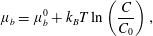
2.3.1 Compressibility: Gibbs ( $E$
) and Marangoni (
$E_{0}$
) moduli
$E$
) and Marangoni (
$E_{0}$
) moduli


The surface compressional (or dilatational) modulus,
 $$\begin{eqnarray}E=-A\frac{\unicode[STIX]{x2202}\unicode[STIX]{x1D6F1}}{\unicode[STIX]{x2202}A},\end{eqnarray}$$
measures the resistance of the surface to compression, completely analogous to 3-D materials. For insoluble surfactants, the number of surfactants in a monolayer does not change during compression, meaning $A$
can be replaced with
$A$
can be replaced with $N/\unicode[STIX]{x1D6E4}$
in (2.21) to give the insoluble dilatational modulus
$N/\unicode[STIX]{x1D6E4}$
in (2.21) to give the insoluble dilatational modulus
 $$\begin{eqnarray}E_{0}=\unicode[STIX]{x1D6E4}\left.\frac{\unicode[STIX]{x2202}\unicode[STIX]{x1D6F1}}{\unicode[STIX]{x2202}\unicode[STIX]{x1D6E4}}\right|_{N}.\end{eqnarray}$$
The nomenclature of (2.21) and (2.22) varies across the surfactant literature, with the names of Gibbs, Marangoni, Gibbs–Marangoni or simply dilatational modulus used for both $E$
and
$E$
and $E_{0}$
. For the purposes of this review, we will consistently call
$E_{0}$
. For the purposes of this review, we will consistently call $E$
the Gibbs modulus and
$E$
the Gibbs modulus and $E_{0}$
the Marangoni modulus.
$E_{0}$
the Marangoni modulus.
The Marangoni modulus $E_{0}$
measures the work done in squeezing surfactant molecules together, and generally increases with surfactant concentration. For example, ideal gas monolayers have Marangoni modulus
$E_{0}$
measures the work done in squeezing surfactant molecules together, and generally increases with surfactant concentration. For example, ideal gas monolayers have Marangoni modulus
 $$\begin{eqnarray}E_{0}^{ideal}=k_{B}T\unicode[STIX]{x1D6E4},\end{eqnarray}$$
with expressions for other isotherms given in table 1. Notably, the Marangoni modulus for the van der Waals isotherm,
 $$\begin{eqnarray}E_{0}^{vdW}=\frac{k_{B}T\unicode[STIX]{x1D6E4}}{(1-\unicode[STIX]{x1D6E4}/\unicode[STIX]{x1D6E4}_{\infty })^{2}}-\unicode[STIX]{x1D6FD}\unicode[STIX]{x1D6E4}^{2},\end{eqnarray}$$
becomes negative for a range of $\unicode[STIX]{x1D6E4}$
whenever
$\unicode[STIX]{x1D6E4}$
whenever $\unicode[STIX]{x1D6FD}\unicode[STIX]{x1D6E4}_{\infty }/k_{B}T>27/4$
. Just like in three dimensions, a monolayer with negative compressibility is mechanically unstable, and undergoes phase separation to a two-phase coexistence between a high-
$\unicode[STIX]{x1D6FD}\unicode[STIX]{x1D6E4}_{\infty }/k_{B}T>27/4$
. Just like in three dimensions, a monolayer with negative compressibility is mechanically unstable, and undergoes phase separation to a two-phase coexistence between a high- $\unicode[STIX]{x1D6E4}$
condensed phase, and a low-
$\unicode[STIX]{x1D6E4}$
condensed phase, and a low- $\unicode[STIX]{x1D6E4}$
expanded phase.
$\unicode[STIX]{x1D6E4}$
expanded phase.
In what follows (§§ 2.4.2 and 3.2), we will find that monolayers (soluble or insoluble) do not always react instantaneously following compression – finite time scales are required for phase transitions to occur, for surfactants to adsorb or desorb to equilibrate with the surrounding bulk fluid, or for surfactant gradients in the surroundings to diffusively relax. In this regard, the Marangoni modulus $E_{0}$
reflects an intrinsic material property, whereas the Gibbs modulus
$E_{0}$
reflects an intrinsic material property, whereas the Gibbs modulus $E$
describes the dynamic response of a macroscopic interface, which additionally depends on the shape, size and time scales of the forcing.
$E$
describes the dynamic response of a macroscopic interface, which additionally depends on the shape, size and time scales of the forcing.
2.3.2 The chemical potential
In preparation for the upcoming transition to soluble surfactants, we discuss one final thermodynamic property of Langmuir monolayers. The chemical potential represents the free energy cost of adding one additional molecule to the monolayer, holding temperature and area constant
 $$\begin{eqnarray}\unicode[STIX]{x1D707}_{s}(\unicode[STIX]{x1D6E4})=\left.\frac{\unicode[STIX]{x2202}{\mathcal{F}}_{s}}{\unicode[STIX]{x2202}N}\right|_{T,A}.\end{eqnarray}$$
The chemical potential of a monolayer of ideal surfactants – as described by (2.8) – is
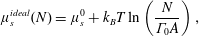 $$\begin{eqnarray}\unicode[STIX]{x1D707}_{s}^{ideal}(N)=\unicode[STIX]{x1D707}_{s}^{0}+k_{B}T\ln \left(\frac{N}{\unicode[STIX]{x1D6E4}_{0}A}\right),\end{eqnarray}$$
or, equivalently,
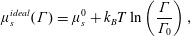 $$\begin{eqnarray}\unicode[STIX]{x1D707}_{s}^{ideal}(\unicode[STIX]{x1D6E4})=\unicode[STIX]{x1D707}_{s}^{0}+k_{B}T\ln \left(\frac{\unicode[STIX]{x1D6E4}}{\unicode[STIX]{x1D6E4}_{0}}\right),\end{eqnarray}$$
where $\unicode[STIX]{x1D707}_{s}^{0}$
is a reference chemical potential, valid at a particular concentration
$\unicode[STIX]{x1D707}_{s}^{0}$
is a reference chemical potential, valid at a particular concentration $\unicode[STIX]{x1D6E4}_{0}$
. In what follows, we will frequently use the Langmuir (lattice) isotherm as a model; its chemical potential is
$\unicode[STIX]{x1D6E4}_{0}$
. In what follows, we will frequently use the Langmuir (lattice) isotherm as a model; its chemical potential is
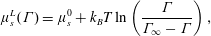 $$\begin{eqnarray}\unicode[STIX]{x1D707}_{s}^{L}(\unicode[STIX]{x1D6E4})=\unicode[STIX]{x1D707}_{s}^{0}+k_{B}T\ln \left(\frac{\unicode[STIX]{x1D6E4}}{\unicode[STIX]{x1D6E4}_{\infty }-\unicode[STIX]{x1D6E4}}\right),\end{eqnarray}$$
where $\unicode[STIX]{x1D707}_{s}^{0}$
is the chemical potential at
$\unicode[STIX]{x1D707}_{s}^{0}$
is the chemical potential at $\unicode[STIX]{x1D6E4}=\unicode[STIX]{x1D6E4}_{\infty }/2$
.
$\unicode[STIX]{x1D6E4}=\unicode[STIX]{x1D6E4}_{\infty }/2$
.
2.4 Soluble surfactants: Gibbs monolayers
We now turn to soluble surfactants, which can dissolve into the liquid below the interface. Monolayers of soluble surfactants – called Gibbs monolayers – represent an equilibrium between surfactants adsorbed at the interface (with surface concentration $\unicode[STIX]{x1D6E4}$
) and those dissolved in the bulk (with concentration
$\unicode[STIX]{x1D6E4}$
) and those dissolved in the bulk (with concentration $C$
).
$C$
).
Detailed balance must hold for adsorbed and dissolved surfactants to be in equilibrium: as many surfactants must adsorb to a surface as desorb in any given time. For this to happen spontaneously, the two states must be equivalent from a free energy standpoint. Adding one surfactant to the monolayer costs energy – the chemical potential $\unicode[STIX]{x1D707}_{s}(\unicode[STIX]{x1D6E4})$
of the adsorbed surfactant. This free energy cost must be identical to the free energy liberated by removing that surfactant from the subphase – represented by the chemical potential
$\unicode[STIX]{x1D707}_{s}(\unicode[STIX]{x1D6E4})$
of the adsorbed surfactant. This free energy cost must be identical to the free energy liberated by removing that surfactant from the subphase – represented by the chemical potential $\unicode[STIX]{x1D707}_{b}(C)$
of the surfactant in the bulk. In short, equilibrium between dissolved and adsorbed surfactant requires
$\unicode[STIX]{x1D707}_{b}(C)$
of the surfactant in the bulk. In short, equilibrium between dissolved and adsorbed surfactant requires
 $$\begin{eqnarray}\unicode[STIX]{x1D707}_{s}(\unicode[STIX]{x1D6E4})=\unicode[STIX]{x1D707}_{b}(C),\end{eqnarray}$$
which defines the equilibrium isotherm $\unicode[STIX]{x1D6E4}(C)$
.
$\unicode[STIX]{x1D6E4}(C)$
.
For example, surfactants that are sufficiently dilute in solution have ‘ideal’ chemical potential
 $$\begin{eqnarray}\unicode[STIX]{x1D707}_{b}=\unicode[STIX]{x1D707}_{b}^{0}+k_{B}T\ln \left(\frac{C}{C_{0}}\right),\end{eqnarray}$$
where $\unicode[STIX]{x1D707}_{b}^{0}$
is the chemical potential at a reference concentration
$\unicode[STIX]{x1D707}_{b}^{0}$
is the chemical potential at a reference concentration $C_{0}$
.
$C_{0}$
.
If adsorbed surfactants also form an ideal gas monolayer, with $\unicode[STIX]{x1D707}_{s}$
given by (2.27), then equating chemical potentials (2.29) reveals a linear relation between adsorbed and bulk concentrations
$\unicode[STIX]{x1D707}_{s}$
given by (2.27), then equating chemical potentials (2.29) reveals a linear relation between adsorbed and bulk concentrations
 $$\begin{eqnarray}\unicode[STIX]{x1D6E4}^{ideal}=\left(\frac{\unicode[STIX]{x1D6E4}_{0}}{C_{0}}\right)\exp \left(\frac{\unicode[STIX]{x1D707}_{b}^{0}-\unicode[STIX]{x1D707}_{s}^{0}}{k_{B}T}\right)C,\end{eqnarray}$$
or
 $$\begin{eqnarray}\unicode[STIX]{x1D6E4}^{ideal}=K^{ideal}C,\end{eqnarray}$$
which is called the Henry isotherm (table 1). Here
 $$\begin{eqnarray}K^{ideal}=\left(\frac{\unicode[STIX]{x1D6E4}_{0}}{C_{0}}\right)\exp \left(\frac{\unicode[STIX]{x1D707}_{b}^{0}-\unicode[STIX]{x1D707}_{s}^{0}}{k_{B}T}\right)\end{eqnarray}$$
is an equilibrium constant for adsorption. The adsorption free energy $\unicode[STIX]{x0394}\unicode[STIX]{x1D707}_{ads}^{0}=\unicode[STIX]{x1D707}_{b}^{0}-\unicode[STIX]{x1D707}_{s}^{0}$
indicates the drop in free energy when a surfactant (at reference concentrations) adsorbs to the interface. As expected from statistical mechanics, the equilibrium constant
$\unicode[STIX]{x0394}\unicode[STIX]{x1D707}_{ads}^{0}=\unicode[STIX]{x1D707}_{b}^{0}-\unicode[STIX]{x1D707}_{s}^{0}$
indicates the drop in free energy when a surfactant (at reference concentrations) adsorbs to the interface. As expected from statistical mechanics, the equilibrium constant $K$
grows exponentially with
$K$
grows exponentially with $\unicode[STIX]{x0394}\unicode[STIX]{x1D707}_{ads}^{0}$
. Different choices of either reference concentration (
$\unicode[STIX]{x0394}\unicode[STIX]{x1D707}_{ads}^{0}$
. Different choices of either reference concentration ( $\unicode[STIX]{x1D6E4}_{0}$
or
$\unicode[STIX]{x1D6E4}_{0}$
or $C_{0}$
), both of which are chosen arbitrarily, would change the corresponding reference chemical potentials (
$C_{0}$
), both of which are chosen arbitrarily, would change the corresponding reference chemical potentials ( $\unicode[STIX]{x1D707}_{s}^{0}$
or
$\unicode[STIX]{x1D707}_{s}^{0}$
or $\unicode[STIX]{x1D707}_{b}^{0}$
, respectively), giving the same adsorption constant
$\unicode[STIX]{x1D707}_{b}^{0}$
, respectively), giving the same adsorption constant $K$
.
$K$
.
Given $\unicode[STIX]{x1D6E4}(C)$
for a Gibbs monolayer of soluble surfactant, other monolayer properties like
$\unicode[STIX]{x1D6E4}(C)$
for a Gibbs monolayer of soluble surfactant, other monolayer properties like $\unicode[STIX]{x1D6F1}(C)$
and
$\unicode[STIX]{x1D6F1}(C)$
and $E_{0}(C)$
can be determined following the thermodynamic arguments for the insoluble surfactants given above. Surface pressure
$E_{0}(C)$
can be determined following the thermodynamic arguments for the insoluble surfactants given above. Surface pressure $\unicode[STIX]{x1D6F1}$
is still defined from the surface free energy via (2.10), so that the Gibbs monolayer defined by (2.32) has
$\unicode[STIX]{x1D6F1}$
is still defined from the surface free energy via (2.10), so that the Gibbs monolayer defined by (2.32) has
 $$\begin{eqnarray}\unicode[STIX]{x1D6F1}^{ideal}=k_{B}TK^{ideal}C,\end{eqnarray}$$
with $K^{ideal}$
defined by (2.33). The Marangoni modulus, defined by (2.22), is also
$K^{ideal}$
defined by (2.33). The Marangoni modulus, defined by (2.22), is also $E_{0}^{ideal}=k_{B}TK^{ideal}C$
.
$E_{0}^{ideal}=k_{B}TK^{ideal}C$
.
More complex isotherms arise for more complex monolayers or solutions. For example, soluble surfactants that adsorb to Langmuir (lattice) monolayers have surface chemical potentials of the Langmuir form (2.28), and equilibrate with an ideal bulk solution of surfactant (2.30) to give
 $$\begin{eqnarray}\frac{\unicode[STIX]{x1D6E4}^{L}}{\unicode[STIX]{x1D6E4}_{\infty }}=\frac{K^{L}C}{1+K^{L}C},\end{eqnarray}$$
where
 $$\begin{eqnarray}K^{L}=\left(\frac{1}{C_{0}}\right)\exp \left(\frac{\unicode[STIX]{x1D707}_{b}^{0}-\unicode[STIX]{x1D707}_{s}^{0}}{k_{B}T}\right)\end{eqnarray}$$
is the equilibrium constant for Langmuir adsorption, with units of $[\text{concentration}]^{-1}$
. The surface pressure for the Langmuir isotherm then follows by inserting
$[\text{concentration}]^{-1}$
. The surface pressure for the Langmuir isotherm then follows by inserting $\unicode[STIX]{x1D6E4}^{L}$
from (2.35) into
$\unicode[STIX]{x1D6E4}^{L}$
from (2.35) into $\unicode[STIX]{x1D6F1}^{L}(\unicode[STIX]{x1D6E4})$
from (2.15) to give
$\unicode[STIX]{x1D6F1}^{L}(\unicode[STIX]{x1D6E4})$
from (2.15) to give
 $$\begin{eqnarray}\unicode[STIX]{x1D6F1}^{L}(C)=k_{B}T\unicode[STIX]{x1D6E4}_{\infty }\log (1+K^{L}C).\end{eqnarray}$$
The desorption constant, $K_{D}^{L}=(K^{L})^{-1}$
, represents a characteristic subphase concentration, at which the interface is half-saturated. The Langmuir adsorption isotherm (2.35) reduces to the ideal gas isotherm (2.34) for concentrations significantly below
$K_{D}^{L}=(K^{L})^{-1}$
, represents a characteristic subphase concentration, at which the interface is half-saturated. The Langmuir adsorption isotherm (2.35) reduces to the ideal gas isotherm (2.34) for concentrations significantly below $K_{D}^{L}$
(i.e.
$K_{D}^{L}$
(i.e. $C\ll 1/K^{L}$
). Similar to insoluble monolayers, adding an interaction term to the surface chemical potential of the Langmuir form gives the Frumkin isotherm. Other models of monolayers that equilibrate with ideal surfactant solutions are reviewed by Kralchevsky et al. (Reference Kralchevsky, Danov and Denkov2008), summarized in table 1 and illustrated in figure 5. All but the (purely empirical) Freundlich isotherm reduce to ideal gas monolayers at sufficiently low
$C\ll 1/K^{L}$
). Similar to insoluble monolayers, adding an interaction term to the surface chemical potential of the Langmuir form gives the Frumkin isotherm. Other models of monolayers that equilibrate with ideal surfactant solutions are reviewed by Kralchevsky et al. (Reference Kralchevsky, Danov and Denkov2008), summarized in table 1 and illustrated in figure 5. All but the (purely empirical) Freundlich isotherm reduce to ideal gas monolayers at sufficiently low $C$
.
$C$
.
Alternatively, surfactants dissolved in solution may show non-ideal behaviour. The most common example is micellization: above a critical micelle concentration (CMC), some surfactants spontaneously aggregate to form micelles. Spherical micelles are most common, but cylinders (‘wormlike micelles’), lamellae and vesicles can also form, depending on molecular morphology and intermolecular forces (Myers Reference Myers2006; Israelachvili Reference Israelachvili2011). The energetics, kinetics, and morphology of micelles is a broad and well-studied topic that is beyond the scope of this review. We will merely point out that at equilibrium and above the CMC, the chemical potential of surfactant monomers, $\unicode[STIX]{x1D707}_{b}(C)$
, must equal the chemical potential of surfactant molecules in micelles,
$\unicode[STIX]{x1D707}_{b}(C)$
, must equal the chemical potential of surfactant molecules in micelles, $\unicode[STIX]{x1D707}_{mic}(C)$
, both of which in turn must equal the chemical potential
$\unicode[STIX]{x1D707}_{mic}(C)$
, both of which in turn must equal the chemical potential $\unicode[STIX]{x1D707}_{s}(\unicode[STIX]{x1D6E4})$
of adsorbed surfactant molecules. In other words, micellization provides an energetic alternative to further interfacial adsorption: once conditions favour micelle formation, adding further surfactant to solution tends to form additional micelles, rather than increase interfacial concentration. Indeed, identifying the bulk concentration at which the surface tension, and ostensibly the surface concentration, becomes approximately constant is a common method for measuring the CMC.
$\unicode[STIX]{x1D707}_{s}(\unicode[STIX]{x1D6E4})$
of adsorbed surfactant molecules. In other words, micellization provides an energetic alternative to further interfacial adsorption: once conditions favour micelle formation, adding further surfactant to solution tends to form additional micelles, rather than increase interfacial concentration. Indeed, identifying the bulk concentration at which the surface tension, and ostensibly the surface concentration, becomes approximately constant is a common method for measuring the CMC.
2.4.1 Gibbs isotherm
It is frequently difficult to measure the surface concentration $\unicode[STIX]{x1D6E4}$
of soluble surfactants; more common is to measure surface pressure
$\unicode[STIX]{x1D6E4}$
of soluble surfactants; more common is to measure surface pressure $\unicode[STIX]{x1D6F1}$
(or, equivalently, surface tension
$\unicode[STIX]{x1D6F1}$
(or, equivalently, surface tension $\unicode[STIX]{x1D6FE}$
) as a function of subphase concentration
$\unicode[STIX]{x1D6FE}$
) as a function of subphase concentration $C$
. In such cases, the Gibbs adsorption isotherm allows
$C$
. In such cases, the Gibbs adsorption isotherm allows $\unicode[STIX]{x1D6E4}$
to be derived from measured
$\unicode[STIX]{x1D6E4}$
to be derived from measured $\unicode[STIX]{x1D6F1}(C)$
relations (Martínez-Balbuena et al.
Reference Martínez-Balbuena, Arteaga-Jiménez, Hernández-Zapata and Márquez-Beltrán2017). The Gibbs relation connects changes in surface pressure
$\unicode[STIX]{x1D6F1}(C)$
relations (Martínez-Balbuena et al.
Reference Martínez-Balbuena, Arteaga-Jiménez, Hernández-Zapata and Márquez-Beltrán2017). The Gibbs relation connects changes in surface pressure $\unicode[STIX]{x1D6F1}$
to changes in the chemical potential
$\unicode[STIX]{x1D6F1}$
to changes in the chemical potential $\unicode[STIX]{x1D707}_{s}$
of adsorbed surfactants at concentration
$\unicode[STIX]{x1D707}_{s}$
of adsorbed surfactants at concentration $\unicode[STIX]{x1D6E4}$
, via (Adamson Reference Adamson1990; Myers Reference Myers2006; Kralchevsky et al.
Reference Kralchevsky, Danov and Denkov2008)
$\unicode[STIX]{x1D6E4}$
, via (Adamson Reference Adamson1990; Myers Reference Myers2006; Kralchevsky et al.
Reference Kralchevsky, Danov and Denkov2008)
 $$\begin{eqnarray}\text{d}\unicode[STIX]{x1D6F1}=-\text{d}\unicode[STIX]{x1D6FE}=\unicode[STIX]{x1D6E4}\,\text{d}\unicode[STIX]{x1D707}_{s}.\end{eqnarray}$$
The chemical potential of adsorbed surfactants $\unicode[STIX]{x1D707}_{s}$
is difficult to determine directly since
$\unicode[STIX]{x1D707}_{s}$
is difficult to determine directly since $\unicode[STIX]{x1D6E4}$
is unknown for soluble surfactants. However, when bulk and adsorbed surfactants are equilibrated,
$\unicode[STIX]{x1D6E4}$
is unknown for soluble surfactants. However, when bulk and adsorbed surfactants are equilibrated, $\unicode[STIX]{x1D707}_{s}$
must be equal to
$\unicode[STIX]{x1D707}_{s}$
must be equal to $\unicode[STIX]{x1D707}_{b}$
for the dissolved surfactants. In cases where the surfactant solution is dilute enough to behave as ideal,
$\unicode[STIX]{x1D707}_{b}$
for the dissolved surfactants. In cases where the surfactant solution is dilute enough to behave as ideal, $\unicode[STIX]{x1D707}_{b}(C)$
is given by (2.30), in which case
$\unicode[STIX]{x1D707}_{b}(C)$
is given by (2.30), in which case
 $$\begin{eqnarray}\text{d}\unicode[STIX]{x1D707}=\text{d}\unicode[STIX]{x1D707}_{s}=k_{B}T\,\text{d}\ln C.\end{eqnarray}$$
The Gibbs relation (2.38) then gives
 $$\begin{eqnarray}\left.\unicode[STIX]{x1D6E4}(C)=\frac{1}{k_{B}T}\frac{\unicode[STIX]{x2202}\unicode[STIX]{x1D6F1}}{\unicode[STIX]{x2202}\ln C}\right|_{T}.\end{eqnarray}$$
In other words, the adsorbed surfactant concentration $\unicode[STIX]{x1D6E4}$
can be determined from measurements of surface pressure
$\unicode[STIX]{x1D6E4}$
can be determined from measurements of surface pressure $\unicode[STIX]{x1D6F1}$
as a function of dissolved surfactant concentration
$\unicode[STIX]{x1D6F1}$
as a function of dissolved surfactant concentration $C$
, so long as the system has equilibrated, and the concentration is well below the CMC (Martínez-Balbuena et al.
Reference Martínez-Balbuena, Arteaga-Jiménez, Hernández-Zapata and Márquez-Beltrán2017).
$C$
, so long as the system has equilibrated, and the concentration is well below the CMC (Martínez-Balbuena et al.
Reference Martínez-Balbuena, Arteaga-Jiménez, Hernández-Zapata and Márquez-Beltrán2017).
2.4.2 Compressibility:
$E$
and
$E_{0}$
for soluble surfactants


The distinction between the Gibbs and Marangoni moduli, $E$
and
$E$
and $E_{0}$
, defined by (2.21) and (2.22) respectively, becomes significant for soluble monolayers. Recall that
$E_{0}$
, defined by (2.21) and (2.22) respectively, becomes significant for soluble monolayers. Recall that $E$
tracks surface pressure changes when the monolayer area
$E$
tracks surface pressure changes when the monolayer area $A$
is changed, whereas
$A$
is changed, whereas $E_{0}$
additionally holds the number
$E_{0}$
additionally holds the number $N$
of adsorbed surfactant molecules fixed – meaning
$N$
of adsorbed surfactant molecules fixed – meaning $\unicode[STIX]{x1D6E4}$
changes when
$\unicode[STIX]{x1D6E4}$
changes when $A$
does. Compressing monolayers of soluble surfactants raises the chemical potential
$A$
does. Compressing monolayers of soluble surfactants raises the chemical potential $\unicode[STIX]{x1D707}_{s}$
of the adsorbed surfactants, without changing the concentration or chemical potential
$\unicode[STIX]{x1D707}_{s}$
of the adsorbed surfactants, without changing the concentration or chemical potential $\unicode[STIX]{x1D707}_{b}(C)$
of the dissolved surfactant. A thermodynamic force drives adsorbed surfactants to desorb, until
$\unicode[STIX]{x1D707}_{b}(C)$
of the dissolved surfactant. A thermodynamic force drives adsorbed surfactants to desorb, until $\unicode[STIX]{x1D6E4}$
returns to the value predicted by (2.29). Once equilibrium is re-established,
$\unicode[STIX]{x1D6E4}$
returns to the value predicted by (2.29). Once equilibrium is re-established, $\unicode[STIX]{x1D6E4}$
returns to its initial value, so that
$\unicode[STIX]{x1D6E4}$
returns to its initial value, so that
 $$\begin{eqnarray}\left.E^{soluble}(t\rightarrow \infty )=-A\frac{\unicode[STIX]{x2202}\unicode[STIX]{x1D6F1}}{\unicode[STIX]{x2202}A}\right|_{t\rightarrow \infty }=0.\end{eqnarray}$$
How quickly the interface re-equilibrates cannot be determined from thermodynamic properties alone, as discussed in § 3.2.
Soluble surfactant monolayers do have a non-zero Marangoni modulus $E_{0}$
, however. After all,
$E_{0}$
, however. After all, $\unicode[STIX]{x1D6E4}$
(and therefore
$\unicode[STIX]{x1D6E4}$
(and therefore $\unicode[STIX]{x1D6F1}$
) must increase during a rapid compression of a Gibbs monolayer, before the surfactants have had the chance to desorb. The Gibbs adsorption equation (2.40), however, offers a route to
$\unicode[STIX]{x1D6F1}$
) must increase during a rapid compression of a Gibbs monolayer, before the surfactants have had the chance to desorb. The Gibbs adsorption equation (2.40), however, offers a route to $E_{0}$
for soluble surfactant monolayers from measured
$E_{0}$
for soluble surfactant monolayers from measured $\unicode[STIX]{x1D6F1}(C)$
isotherms
$\unicode[STIX]{x1D6F1}(C)$
isotherms
 $$\begin{eqnarray}E_{0}=\unicode[STIX]{x1D6E4}\frac{\unicode[STIX]{x2202}\unicode[STIX]{x1D6F1}}{\unicode[STIX]{x2202}\unicode[STIX]{x1D6E4}}=\unicode[STIX]{x1D6E4}\frac{\unicode[STIX]{x2202}\unicode[STIX]{x1D6F1}}{\unicode[STIX]{x2202}\ln C}\frac{\unicode[STIX]{x2202}\ln C}{\unicode[STIX]{x2202}\unicode[STIX]{x1D6E4}}.\end{eqnarray}$$
Substituting $\unicode[STIX]{x1D6E4}$
and
$\unicode[STIX]{x1D6E4}$
and $\unicode[STIX]{x2202}\unicode[STIX]{x1D6E4}/\unicode[STIX]{x2202}\ln C$
using (2.40) gives
$\unicode[STIX]{x2202}\unicode[STIX]{x1D6E4}/\unicode[STIX]{x2202}\ln C$
using (2.40) gives
 $$\begin{eqnarray}E_{0}=\frac{(\unicode[STIX]{x1D6F1}^{\prime })^{2}}{\unicode[STIX]{x1D6F1}^{\prime \prime }},\quad \text{or}\quad \frac{1}{E_{0}}=-\left(\frac{1}{\unicode[STIX]{x1D6F1}^{\prime }}\right)^{\prime },\end{eqnarray}$$
where primes denote differentiation with respect to $\ln C$
.
$\ln C$
.
While the Gibbs modulus $E$
describes the monolayer’s mechanical response to macroscopic compression or expansion
$E$
describes the monolayer’s mechanical response to macroscopic compression or expansion $(dA)$
, the Marangoni modulus
$(dA)$
, the Marangoni modulus $E_{0}$
reflects sensitivity to intrinsic molecular concentrations
$E_{0}$
reflects sensitivity to intrinsic molecular concentrations $\unicode[STIX]{x1D6E4}$
, and will play an important role in establishing an effective surface dilatational viscosity for surfactant monolayers, as shown in § 4.2.
$\unicode[STIX]{x1D6E4}$
, and will play an important role in establishing an effective surface dilatational viscosity for surfactant monolayers, as shown in § 4.2.
2.4.3 Soluble isotherms via dynamic equilibrium
Equilibrium between surfactants adsorbed at an interface and dissolved in the subphase can also be determined by explicitly balancing adsorption and desorption fluxes. This approach holds particular value to the fluid mechanics community, as it connects the equilibrium arguments and measurements made above to Marangoni stresses and dynamical processes in surfactant systems.
The simplest expressions for adsorption and desorption fluxes – which one should expect to hold for ideal mixtures in both the monolayer and in the bulk – is to take the adsorption flux, $j_{a}$
, to be proportional to the bulk concentration
$j_{a}$
, to be proportional to the bulk concentration $C$
, and the desorption flux
$C$
, and the desorption flux $j_{d}$
to be proportional to the adsorbed concentration
$j_{d}$
to be proportional to the adsorbed concentration $\unicode[STIX]{x1D6E4}$
:
$\unicode[STIX]{x1D6E4}$
:
 $$\begin{eqnarray}\displaystyle & \displaystyle j_{a}=k_{a}C, & \displaystyle\end{eqnarray}$$
 $$\begin{eqnarray}\displaystyle & \displaystyle j_{d}=k_{d}\unicode[STIX]{x1D6E4}. & \displaystyle\end{eqnarray}$$
These fluxes balance at equilibrium, $j_{a}=j_{d}$
, giving
$j_{a}=j_{d}$
, giving
 $$\begin{eqnarray}\unicode[STIX]{x1D6E4}^{ideal}=\frac{k_{a}}{k_{d}}C\equiv K^{ideal}C,\end{eqnarray}$$
reproducing the Henry isotherm (2.32). Previously, the adsorption constant $K^{ideal}$
was shown to depend upon the free energy of adsorption
$K^{ideal}$
was shown to depend upon the free energy of adsorption $\unicode[STIX]{x0394}\unicode[STIX]{x1D707}=\unicode[STIX]{x1D707}_{b}^{0}-\unicode[STIX]{x1D707}_{s}^{0}$
via (2.33). Equation (2.46) additionally relates
$\unicode[STIX]{x0394}\unicode[STIX]{x1D707}=\unicode[STIX]{x1D707}_{b}^{0}-\unicode[STIX]{x1D707}_{s}^{0}$
via (2.33). Equation (2.46) additionally relates $K^{ideal}$
to the ratio of adsorptive to desorptive rate constants
$K^{ideal}$
to the ratio of adsorptive to desorptive rate constants $k_{a}/k_{d}$
. Each individual rate constant
$k_{a}/k_{d}$
. Each individual rate constant $k_{a}$
and
$k_{a}$
and $k_{d}$
cannot be determined from an equilibrium quantity like
$k_{d}$
cannot be determined from an equilibrium quantity like $K$
; however, the ratio of the two is set by thermodynamics.
$K$
; however, the ratio of the two is set by thermodynamics.
Other isotherms require different adsorption and/or desorption rate kinetics. For example, the Langmuir isotherm (2.35) is formed when dissolved surfactants adsorb to vacant lattice sites (Levich Reference Levich1962; Adamson Reference Adamson1990; Kralchevsky et al. Reference Kralchevsky, Danov and Denkov2008), modifying the adsorption flux (2.44) to
 $$\begin{eqnarray}j_{a}^{\,L}=k_{a}C(\unicode[STIX]{x1D6E4}_{\infty }-\unicode[STIX]{x1D6E4}).\end{eqnarray}$$
At equilibrium, $j_{a}^{L}=j_{d}$
, so that
$j_{a}^{L}=j_{d}$
, so that
 $$\begin{eqnarray}\frac{k_{a}C}{k_{d}}=\frac{\unicode[STIX]{x1D6E4}^{L}}{\unicode[STIX]{x1D6E4}_{\infty }-\unicode[STIX]{x1D6E4}^{L}},\end{eqnarray}$$
recovering (2.35) with $K=k_{a}/k_{d}$
. Adsorption and desorption fluxes for other common isotherms are listed in table 2.
$K=k_{a}/k_{d}$
. Adsorption and desorption fluxes for other common isotherms are listed in table 2.
Table 2. Example adsorption and desorption fluxes for the isotherms detailed in table 1. Because only the ratio of $j_{a}$
and
$j_{a}$
and $j_{d}$
is constrained by equilibrium thermodynamics, each pair (
$j_{d}$
is constrained by equilibrium thermodynamics, each pair ( $j_{a}$
and
$j_{a}$
and $j_{d}$
) in this table may be multiplied by any function of
$j_{d}$
) in this table may be multiplied by any function of $C$
and
$C$
and $\unicode[STIX]{x1D6E4}$
without changing its equilibrium isotherm. Different surfactants with identical isotherms may respond very differently under dynamic conditions.
$\unicode[STIX]{x1D6E4}$
without changing its equilibrium isotherm. Different surfactants with identical isotherms may respond very differently under dynamic conditions.

This dynamic equilibrium approach forms a natural transition into § 3, which addresses the dynamic response of surfactant-laden interfaces when they are driven out of equilibrium. Specifically, we will describe how fluid flow transports surfactant molecules in the bulk and on the interface, and how the tendency of surfactant molecules to re-equilibrate in turn impacts interfacial fluid dynamics.
3 Dynamic properties
So far, we have assumed that interfacial deformations have been ‘slow enough’, or that we have waited long enough, that the surfactants have remained in quasi-steady equilibrium, instantaneously redistributing and/or adsorbing and desorbing to equilibrate with the bulk liquid beneath them. However, these processes take time. Various dynamic surfactant processes arise in systems driven out of equilibrium, modifying the behaviour of even the simplest systems. Figure 1, for example, highlights the dynamic surfactant processes that impact a rising gas bubble. Convective flow along the fluid interface sweeps surfactants to the rear as the bubble rises. The resulting concentration gradients generate Marangoni stresses that act to oppose the motion that created them. Surface diffusion smooths out non-uniform distributions of surface concentration, as does surfactant exchange with the bulk, thereby reducing the strength of Marangoni flows. Additionally, surface excess rheological stresses might arise as insoluble surfactant monolayers are sheared or compressed.
Interpreting, predicting and engineering these surfactant systems then necessitates a thorough understanding of the interplay between physically distinct transport processes. Our objective in this section is to provide an introduction to the physics and the mathematical machinery that govern the out-of-equilibrium behaviour of surfactant systems. We will start with the governing equations of surfactant transport (§ 3.1), discuss the competition between diffusion and adsorption/desorption kinetics in surfactant exchange between bulk and adsorbed states (§ 3.2), outline the origins of Marangoni stresses and characterize its strength relative to other processes (§ 3.3) and finally describe the fluid mechanics of systems with a non-zero surface excess viscosities (§ 3.4).
3.1 Governing equations
Our discussion thus far has centred on the equilibrium properties of surfactants. Of particular interest to the fluid dynamics community, on the other hand, is the coupling between the surfactants and the fluids surrounding the interface. Conservation equations for the mass and momentum of the bulk fluid are well known,
 $$\begin{eqnarray}\displaystyle & \displaystyle \unicode[STIX]{x1D70C}\,\frac{\text{D}\boldsymbol{v}}{\text{D}t}=-\unicode[STIX]{x1D735}p+\unicode[STIX]{x1D702}\unicode[STIX]{x1D6FB}^{2}\boldsymbol{v}, & \displaystyle\end{eqnarray}$$
 $$\begin{eqnarray}\displaystyle & \displaystyle \unicode[STIX]{x1D735}\boldsymbol{\cdot }\boldsymbol{v}=0, & \displaystyle\end{eqnarray}$$ $\unicode[STIX]{x1D70C}$
the fluid density,
$\unicode[STIX]{x1D70C}$
the fluid density, $\unicode[STIX]{x1D702}$
the shear viscosity,
$\unicode[STIX]{x1D702}$
the shear viscosity, $\boldsymbol{v}$
the fluid velocity and
$\boldsymbol{v}$
the fluid velocity and $p$
the pressure.
$p$
the pressure.
At first glance, boundary conditions seem to be fairly straightforward. The kinematic boundary condition relates the fluid velocity normal to an interface to the deformation velocity of that interface (Leal Reference Leal2007): a fluid interface located at $\boldsymbol{r}_{s}(t)$
is defined by
$\boldsymbol{r}_{s}(t)$
is defined by
 $$\begin{eqnarray}\unicode[STIX]{x1D6F7}(\boldsymbol{r}_{s},t)=0,\end{eqnarray}$$
with unit normal
 $$\begin{eqnarray}\boldsymbol{n}=\left.\frac{\unicode[STIX]{x1D735}\unicode[STIX]{x1D6F7}}{|\unicode[STIX]{x1D735}\unicode[STIX]{x1D6F7}|}\right|_{\boldsymbol{r}_{s}},\end{eqnarray}$$
and requires
 $$\begin{eqnarray}\boldsymbol{n}\boldsymbol{\cdot }\boldsymbol{v}(\boldsymbol{r}_{s})=-\left.\frac{1}{|\unicode[STIX]{x1D735}\unicode[STIX]{x1D6F7}|}\frac{\unicode[STIX]{x2202}\unicode[STIX]{x1D6F7}}{\unicode[STIX]{x2202}t}\right|_{\boldsymbol{r}_{s}}.\end{eqnarray}$$
Likewise, the fluid velocity at the interface, $\boldsymbol{u}$
, generally obeys the no-slip condition
$\boldsymbol{u}$
, generally obeys the no-slip condition
 $$\begin{eqnarray}\boldsymbol{u}(\boldsymbol{r}_{s})=\boldsymbol{v}(\boldsymbol{r}_{s}).\end{eqnarray}$$
In general, the stress boundary condition is more complicated. Conservation of momentum at the interface gives (Slattery, Sagis & Oh Reference Slattery, Sagis and Oh2007)
 $$\begin{eqnarray}\unicode[STIX]{x1D70C}_{s}\frac{\text{D}\boldsymbol{u}}{\text{D}t}=\boldsymbol{n}\boldsymbol{\cdot }[\![\unicode[STIX]{x1D748}]\!]+\unicode[STIX]{x1D735}_{s}\boldsymbol{\cdot }\unicode[STIX]{x1D748}_{s},\end{eqnarray}$$
where $\unicode[STIX]{x1D70C}_{s}$
is the surface mass density,
$\unicode[STIX]{x1D70C}_{s}$
is the surface mass density, $[\![\unicode[STIX]{x1D748}]\!]=\unicode[STIX]{x1D748}_{upper}-\unicode[STIX]{x1D748}_{lower}$
is the hydrodynamic stress jump across the interface with
$[\![\unicode[STIX]{x1D748}]\!]=\unicode[STIX]{x1D748}_{upper}-\unicode[STIX]{x1D748}_{lower}$
is the hydrodynamic stress jump across the interface with $\boldsymbol{n}$
pointing into the ‘upper’ fluid and
$\boldsymbol{n}$
pointing into the ‘upper’ fluid and $\unicode[STIX]{x1D735}_{s}=(\unicode[STIX]{x1D644}-\boldsymbol{n}\boldsymbol{n})\boldsymbol{\cdot }\unicode[STIX]{x1D735}$
is the surface gradient operator. The surface stress tensor is
$\unicode[STIX]{x1D735}_{s}=(\unicode[STIX]{x1D644}-\boldsymbol{n}\boldsymbol{n})\boldsymbol{\cdot }\unicode[STIX]{x1D735}$
is the surface gradient operator. The surface stress tensor is
 $$\begin{eqnarray}\unicode[STIX]{x1D748}_{s}=\unicode[STIX]{x1D6FE}\unicode[STIX]{x1D644}_{s}+\unicode[STIX]{x1D749}_{rheol},\end{eqnarray}$$
where $\unicode[STIX]{x1D6FE}$
is the local surface tension,
$\unicode[STIX]{x1D6FE}$
is the local surface tension, $\unicode[STIX]{x1D644}_{s}=\unicode[STIX]{x1D644}-\boldsymbol{n}\boldsymbol{n}$
is the surface identity tensor and we have included surface rheological stresses
$\unicode[STIX]{x1D644}_{s}=\unicode[STIX]{x1D644}-\boldsymbol{n}\boldsymbol{n}$
is the surface identity tensor and we have included surface rheological stresses $\unicode[STIX]{x1D749}_{rheol}$
in anticipation, but defer detailed discussion to § 3.4.
$\unicode[STIX]{x1D749}_{rheol}$
in anticipation, but defer detailed discussion to § 3.4.
Neglecting fluid and surfactant inertia, the interfacial stress balance (3.6) becomes
 $$\begin{eqnarray}-\boldsymbol{n}\boldsymbol{\cdot }[\![\unicode[STIX]{x1D748}]\!]=\unicode[STIX]{x1D735}_{s}\unicode[STIX]{x1D6FE}-\unicode[STIX]{x1D6FE}(\unicode[STIX]{x1D735}_{s}\boldsymbol{\cdot }\boldsymbol{n})\boldsymbol{n}+\unicode[STIX]{x1D735}_{s}\boldsymbol{\cdot }\unicode[STIX]{x1D749}_{rheol}.\end{eqnarray}$$
The tangential component of (3.8) reveals that imbalances between viscous shear stress can be driven by (or balance) both Marangoni stresses (§ 3.3) and surface rheological stresses (§ 3.4). The normal component of (3.8) reduces to the Young–Laplace equation (2.6) in a static system ( $\unicode[STIX]{x1D748}=-p\,\unicode[STIX]{x1D644}$
) if surface rheological stresses are absent.
$\unicode[STIX]{x1D748}=-p\,\unicode[STIX]{x1D644}$
) if surface rheological stresses are absent.
The interfacial stress boundary condition (3.8) depends on the surface tension $\unicode[STIX]{x1D6FE}$
(or surface pressure
$\unicode[STIX]{x1D6FE}$
(or surface pressure $\unicode[STIX]{x1D6F1}$
), which in turn depends on adsorbed surfactant concentration
$\unicode[STIX]{x1D6F1}$
), which in turn depends on adsorbed surfactant concentration $\unicode[STIX]{x1D6E4}(\boldsymbol{r}_{s},t)$
via some isotherm, as described in § 2.3. Still, the concentration profile of adsorbed surfactant
$\unicode[STIX]{x1D6E4}(\boldsymbol{r}_{s},t)$
via some isotherm, as described in § 2.3. Still, the concentration profile of adsorbed surfactant $\unicode[STIX]{x1D6E4}$
changes in space and time, and must therefore be determined. To do so requires addressing dynamic questions of surfactant transport: convective and diffusive transport along the interface, adsorption and desorption of surfactant between the interface and the bulk solution(s).
$\unicode[STIX]{x1D6E4}$
changes in space and time, and must therefore be determined. To do so requires addressing dynamic questions of surfactant transport: convective and diffusive transport along the interface, adsorption and desorption of surfactant between the interface and the bulk solution(s).
Adsorbed surfactant evolves according to a conservation equation
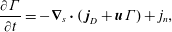 $$\begin{eqnarray}\frac{\unicode[STIX]{x2202}\unicode[STIX]{x1D6E4}}{\unicode[STIX]{x2202}t}=-\unicode[STIX]{x1D735}_{s}\boldsymbol{\cdot }(\boldsymbol{j}_{D}+\boldsymbol{u}\unicode[STIX]{x1D6E4})+j_{n},\end{eqnarray}$$
where $\boldsymbol{j}_{D}$
represents the diffusive flux along the interface, and
$\boldsymbol{j}_{D}$
represents the diffusive flux along the interface, and $\boldsymbol{u}\unicode[STIX]{x1D6E4}$
represents the surface advective flux. The final term
$\boldsymbol{u}\unicode[STIX]{x1D6E4}$
represents the surface advective flux. The final term $j_{n}$
accounts for the local ‘production’ or ‘consumption’ of adsorbed surfactant, typically driven by adsorptive and desorptive exchange between the bulk solution and the interface. If more surfactant adsorbs to a spot on the interface than desorbs from that spot, then
$j_{n}$
accounts for the local ‘production’ or ‘consumption’ of adsorbed surfactant, typically driven by adsorptive and desorptive exchange between the bulk solution and the interface. If more surfactant adsorbs to a spot on the interface than desorbs from that spot, then $\unicode[STIX]{x1D6E4}$
grows (and
$\unicode[STIX]{x1D6E4}$
grows (and $j_{n}>0$
) at that spot.
$j_{n}>0$
) at that spot.
A common form of this equation, as formally derived by Aris (Reference Aris1962) and Stone (Reference Stone1990), assumes constant surface diffusivity $D_{s}$
, and reads
$D_{s}$
, and reads
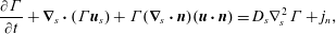 $$\begin{eqnarray}\frac{\unicode[STIX]{x2202}\unicode[STIX]{x1D6E4}}{\unicode[STIX]{x2202}t}+\unicode[STIX]{x1D735}_{s}\boldsymbol{\cdot }(\unicode[STIX]{x1D6E4}\boldsymbol{u}_{s})+\unicode[STIX]{x1D6E4}(\unicode[STIX]{x1D735}_{s}\boldsymbol{\cdot }\boldsymbol{n})(\boldsymbol{u}\boldsymbol{\cdot }\boldsymbol{n})=D_{s}\unicode[STIX]{x1D6FB}_{s}^{2}\unicode[STIX]{x1D6E4}+j_{n},\end{eqnarray}$$
where $\boldsymbol{u}_{s}$
is the in-plane surface velocity
$\boldsymbol{u}_{s}$
is the in-plane surface velocity
 $$\begin{eqnarray}\boldsymbol{u}_{s}=(\unicode[STIX]{x1D644}-\boldsymbol{n}\boldsymbol{n})\boldsymbol{\cdot }\boldsymbol{v}(\boldsymbol{r}_{s})=(\unicode[STIX]{x1D644}-\boldsymbol{n}\boldsymbol{n})\boldsymbol{\cdot }\boldsymbol{u}.\end{eqnarray}$$
In what follows, we will discuss subtleties and assumptions built into this expression, as well as generalizations.
3.1.1 Surface advection
The surface advective flux can be decomposed into components normal to the interface, and components along the interface
 $$\begin{eqnarray}\boldsymbol{u}\unicode[STIX]{x1D6E4}=\boldsymbol{n}(\boldsymbol{n}\boldsymbol{\cdot }\boldsymbol{u})\unicode[STIX]{x1D6E4}+(\unicode[STIX]{x1D644}-\boldsymbol{n}\boldsymbol{n})\boldsymbol{\cdot }\boldsymbol{u}\unicode[STIX]{x1D6E4},\end{eqnarray}$$
and therefore has surface divergence
 $$\begin{eqnarray}\unicode[STIX]{x1D735}_{s}\boldsymbol{\cdot }(\boldsymbol{u}\unicode[STIX]{x1D6E4})=\unicode[STIX]{x1D6E4}(\unicode[STIX]{x1D735}_{s}\boldsymbol{\cdot }\boldsymbol{n})(\boldsymbol{u}\boldsymbol{\cdot }\boldsymbol{n})+\unicode[STIX]{x1D735}_{s}\boldsymbol{\cdot }(\boldsymbol{u}_{s}\unicode[STIX]{x1D6E4}),\end{eqnarray}$$
as in (3.10). The first term captures the compression or dilation of surfactant that occurs when curved interfaces ( $\unicode[STIX]{x1D735}_{s}\boldsymbol{\cdot }\boldsymbol{n}\neq 0$
) themselves deform (due to non-zero normal interfacial velocities), and the second term captures the compression or dilation arising from non-uniform convective flux within the plane of the interface.
$\unicode[STIX]{x1D735}_{s}\boldsymbol{\cdot }\boldsymbol{n}\neq 0$
) themselves deform (due to non-zero normal interfacial velocities), and the second term captures the compression or dilation arising from non-uniform convective flux within the plane of the interface.
3.1.2 Surface diffusion
The standard expression for the diffusive flux of adsorbed surfactant along a surface, used to derive (3.10), has a Fickian form,
 $$\begin{eqnarray}\boldsymbol{j}_{D}^{\,Fick}=-D_{s}\unicode[STIX]{x1D735}_{s}\unicode[STIX]{x1D6E4},\end{eqnarray}$$
A diffusive flux of this form, however, is built on assumptions that are rarely accurate in systems of practical interest.
A brief derivation of the diffusive flux highlights conditions under which the Fickian form holds. Because the chemical potential $\unicode[STIX]{x1D707}(\unicode[STIX]{x1D6E4},T)$
represents the free energy ‘cost’ of an adsorbed surfactant at concentration
$\unicode[STIX]{x1D707}(\unicode[STIX]{x1D6E4},T)$
represents the free energy ‘cost’ of an adsorbed surfactant at concentration $\unicode[STIX]{x1D6E4}$
and temperature
$\unicode[STIX]{x1D6E4}$
and temperature $T$
, any spatial gradients in
$T$
, any spatial gradients in $\unicode[STIX]{x1D707}$
point toward more ‘costly’ locations for surfactants to be placed. A chemical potential gradient thus represents a thermodynamic force (
$\unicode[STIX]{x1D707}$
point toward more ‘costly’ locations for surfactants to be placed. A chemical potential gradient thus represents a thermodynamic force ( $\boldsymbol{f}_{s}=-\unicode[STIX]{x1D735}_{s}\unicode[STIX]{x1D707}$
) on an adsorbed surfactant, which drives it to migrate along the interface, with relative velocity
$\boldsymbol{f}_{s}=-\unicode[STIX]{x1D735}_{s}\unicode[STIX]{x1D707}$
) on an adsorbed surfactant, which drives it to migrate along the interface, with relative velocity
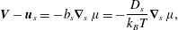 $$\begin{eqnarray}\boldsymbol{V}-\boldsymbol{u}_{s}=-b_{s}\unicode[STIX]{x1D735}_{s}\unicode[STIX]{x1D707}=-\frac{D_{s}}{k_{B}T}\unicode[STIX]{x1D735}_{s}\unicode[STIX]{x1D707},\end{eqnarray}$$
where $b_{s}$
is the hydrodynamic mobility of the surfactant along the surface, and is related to its self-diffusivity by the Stokes–Einstein relation (Saffman & Delbrück Reference Saffman and Delbrück1975; Furst & Squires Reference Furst and Squires2017)
$b_{s}$
is the hydrodynamic mobility of the surfactant along the surface, and is related to its self-diffusivity by the Stokes–Einstein relation (Saffman & Delbrück Reference Saffman and Delbrück1975; Furst & Squires Reference Furst and Squires2017)
 $$\begin{eqnarray}D_{s}=k_{B}Tb_{s}.\end{eqnarray}$$
Each surfactant molecule moves with velocity (3.15) along the surface, so that a single-component monolayer of surface concentration $\unicode[STIX]{x1D6E4}$
establishes a flux
$\unicode[STIX]{x1D6E4}$
establishes a flux
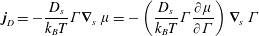 $$\begin{eqnarray}\boldsymbol{j}_{D}=-\frac{D_{s}}{k_{B}T}\unicode[STIX]{x1D6E4}\unicode[STIX]{x1D735}_{s}\unicode[STIX]{x1D707}=-\left(\frac{D_{s}}{k_{B}T}\unicode[STIX]{x1D6E4}\frac{\unicode[STIX]{x2202}\unicode[STIX]{x1D707}}{\unicode[STIX]{x2202}\unicode[STIX]{x1D6E4}}\right)\unicode[STIX]{x1D735}_{s}\unicode[STIX]{x1D6E4}\end{eqnarray}$$
relative to the interface. In multi-component monolayers, the chemical potential of each species depends on the surface concentration of every other component, and the term in brackets in (3.17) is replaced by a generalized Maxwell–Stefan diffusivity tensor (Krishna Reference Krishna1990). In what follows, we restrict our discussion to single-component monolayers.
The Fickian form (3.14) holds only for the ideal gas monolayer, for which $\unicode[STIX]{x1D707}=\unicode[STIX]{x1D707}_{s}^{ideal}(\unicode[STIX]{x1D6E4})$
from (2.27), and therefore
$\unicode[STIX]{x1D707}=\unicode[STIX]{x1D707}_{s}^{ideal}(\unicode[STIX]{x1D6E4})$
from (2.27), and therefore
 $$\begin{eqnarray}\frac{\unicode[STIX]{x2202}\unicode[STIX]{x1D707}_{s}^{ideal}}{\unicode[STIX]{x2202}\unicode[STIX]{x1D6E4}}=\frac{k_{B}T}{\unicode[STIX]{x1D6E4}},\end{eqnarray}$$
so that the diffusive flux (3.17) reduces to Fick’s law (3.14). As discussed in § 2.3, however, it is rare for any surfactant that reduces surface tension in any appreciable way to behave as an ideal gas. The Fickian form, then, rarely holds as explicitly derived. Of course, one can define an effective diffusivity
 $$\begin{eqnarray}D_{s}^{eff}(\unicode[STIX]{x1D6E4})=\frac{D_{s}}{k_{B}T}\unicode[STIX]{x1D6E4}\frac{\unicode[STIX]{x2202}\unicode[STIX]{x1D707}}{\unicode[STIX]{x2202}\unicode[STIX]{x1D6E4}},\end{eqnarray}$$
which differs from the true self-diffusivity of each surfactant molecule. If gradients are small enough that $D_{s}^{eff}$
is approximately constant, then the Fickian form would be appropriate, albeit with a modified diffusivity.
$D_{s}^{eff}$
is approximately constant, then the Fickian form would be appropriate, albeit with a modified diffusivity.
The effective surface diffusivity $D_{s}^{eff}$
can be shown using (2.22) and (2.23) to exceed the Fickian self-diffusivity by the Marangoni modulus
$D_{s}^{eff}$
can be shown using (2.22) and (2.23) to exceed the Fickian self-diffusivity by the Marangoni modulus $E_{0}(\unicode[STIX]{x1D6E4})$
relative to an ideal gas monolayer
$E_{0}(\unicode[STIX]{x1D6E4})$
relative to an ideal gas monolayer
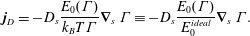 $$\begin{eqnarray}\boldsymbol{j}_{D}=-D_{s}\frac{E_{0}(\unicode[STIX]{x1D6E4})}{k_{B}T\unicode[STIX]{x1D6E4}}\unicode[STIX]{x1D735}_{s}\unicode[STIX]{x1D6E4}\equiv -D_{s}\frac{E_{0}(\unicode[STIX]{x1D6E4})}{E_{0}^{ideal}}\unicode[STIX]{x1D735}_{s}\unicode[STIX]{x1D6E4}.\end{eqnarray}$$
The diffusive flux expressions for the Langmuir and Volmer isotherms (table 1), for example, become
 $$\begin{eqnarray}\boldsymbol{j}_{D}^{L}=-\frac{D_{s}}{1-\unicode[STIX]{x1D6E4}/\unicode[STIX]{x1D6E4}_{\infty }}\unicode[STIX]{x1D735}_{s}\unicode[STIX]{x1D6E4}\quad \text{and}\quad \boldsymbol{j}_{D}^{V}=-\frac{D_{s}}{(1-\unicode[STIX]{x1D6E4}/\unicode[STIX]{x1D6E4}_{\infty })^{2}}\unicode[STIX]{x1D735}_{s}\unicode[STIX]{x1D6E4}.\end{eqnarray}$$
Curiously, the diffusive flux of adsorbed surfactant within single-component monolayers can be expressed in terms of surface pressure gradients alone. The Gibbs adsorption relation (2.38) directly implies
 $$\begin{eqnarray}\unicode[STIX]{x1D6E4}\unicode[STIX]{x1D735}_{s}\unicode[STIX]{x1D707}=\unicode[STIX]{x1D735}_{s}\unicode[STIX]{x1D6F1},\end{eqnarray}$$
which can be substituted for $\unicode[STIX]{x1D6E4}\unicode[STIX]{x1D735}_{s}\unicode[STIX]{x1D707}$
in (3.17) to give a diffusive flux
$\unicode[STIX]{x1D6E4}\unicode[STIX]{x1D735}_{s}\unicode[STIX]{x1D707}$
in (3.17) to give a diffusive flux
 $$\begin{eqnarray}\boldsymbol{j}_{D}=-b_{s}\unicode[STIX]{x1D735}_{s}\unicode[STIX]{x1D6F1},\end{eqnarray}$$
which appears to be independent of the surface concentration $\unicode[STIX]{x1D6E4}$
! Although this result seems counter-intuitive at first, it can be understood physically as follows. The surface pressure gradient gives the force per unit area exerted on the surfactant monolayer, which is divided among
$\unicode[STIX]{x1D6E4}$
! Although this result seems counter-intuitive at first, it can be understood physically as follows. The surface pressure gradient gives the force per unit area exerted on the surfactant monolayer, which is divided among $\unicode[STIX]{x1D6E4}$
molecules per unit area. The greater the concentration
$\unicode[STIX]{x1D6E4}$
molecules per unit area. The greater the concentration $\unicode[STIX]{x1D6E4}$
of adsorbed surfactant, the weaker the force on each (
$\unicode[STIX]{x1D6E4}$
of adsorbed surfactant, the weaker the force on each ( $\boldsymbol{F}_{s}\sim \unicode[STIX]{x1D6FB}\unicode[STIX]{x1D6F1}/\unicode[STIX]{x1D6E4}$
), and the slower each migrates:
$\boldsymbol{F}_{s}\sim \unicode[STIX]{x1D6FB}\unicode[STIX]{x1D6F1}/\unicode[STIX]{x1D6E4}$
), and the slower each migrates: $\boldsymbol{V}\sim b_{s}(\unicode[STIX]{x1D735}_{s}\unicode[STIX]{x1D6F1}/\unicode[STIX]{x1D6E4})$
. Ultimately, the concentration
$\boldsymbol{V}\sim b_{s}(\unicode[STIX]{x1D735}_{s}\unicode[STIX]{x1D6F1}/\unicode[STIX]{x1D6E4})$
. Ultimately, the concentration $\unicode[STIX]{x1D6E4}$
cancels out of the flux
$\unicode[STIX]{x1D6E4}$
cancels out of the flux $\unicode[STIX]{x1D6E4}\boldsymbol{V}$
in (3.23).
$\unicode[STIX]{x1D6E4}\boldsymbol{V}$
in (3.23).

Figure 6. (a) Geometry of a typical surfactant-laden interface. (b–e) Mass transport processes on the interface: (b) convection due to imposed (or Marangoni) velocity $u_{s}$
; (c) diffusion due to a surface concentration gradient; (d) surface concentration evolution due to curvature modification; and (e) adsorption/desorption from the sublayer, showing the depletion length
$u_{s}$
; (c) diffusion due to a surface concentration gradient; (d) surface concentration evolution due to curvature modification; and (e) adsorption/desorption from the sublayer, showing the depletion length $L_{d}$
.
$L_{d}$
.
3.2 Adsorption/desorption
The final term in the surfactant conservation equation, $j_{n}$
, accounts for exchange of molecules between the bulk and the interface. At equilibrium, adsorption and desorption fluxes balance each other (§ 2.4.3). For an interface out of equilibrium, the difference between
$j_{n}$
, accounts for exchange of molecules between the bulk and the interface. At equilibrium, adsorption and desorption fluxes balance each other (§ 2.4.3). For an interface out of equilibrium, the difference between $j_{a}$
and
$j_{a}$
and $j_{d}$
represents a kinetic flux of surfactant entering or leaving the interface
$j_{d}$
represents a kinetic flux of surfactant entering or leaving the interface
 $$\begin{eqnarray}j_{kin}=j_{a}(\unicode[STIX]{x1D6E4},C_{s})-j_{d}(\unicode[STIX]{x1D6E4},C_{s}),\end{eqnarray}$$
where
 $$\begin{eqnarray}C_{s}=C(\boldsymbol{r}_{s},t)\end{eqnarray}$$
is the surfactant concentration in the bulk fluid, evaluated at the interface (figure 6
e). Table 2 gives $j_{a}$
and
$j_{a}$
and $j_{d}$
corresponding to the common isotherms described in § 2.3 and table 1.
$j_{d}$
corresponding to the common isotherms described in § 2.3 and table 1.
Departures from a constant equilibrium concentration $C_{0}$
also drive surfactant transport in the bulk, governed by the convection–diffusion equation
$C_{0}$
also drive surfactant transport in the bulk, governed by the convection–diffusion equation
 $$\begin{eqnarray}\frac{\unicode[STIX]{x2202}C}{\unicode[STIX]{x2202}t}=D\unicode[STIX]{x1D6FB}^{2}C-\boldsymbol{v}\boldsymbol{\cdot }\unicode[STIX]{x1D735}C.\end{eqnarray}$$
Concentration gradients in the bulk may drive a diffusive flux of surfactants onto or off the interface, via
 $$\begin{eqnarray}j_{diff}=D\boldsymbol{n}\boldsymbol{\cdot }\unicode[STIX]{x1D735}C|_{\boldsymbol{r}_{s}},\end{eqnarray}$$
where $\boldsymbol{n}$
is normal to the interface and points into the bulk fluid containing the surfactant. Surfactant conservation requires this diffusive flux (3.27) to balance the kinetic flux of adsorption/desorption to the interface (3.24), both of which equal the source term in the surface conservation equation (3.10):
$\boldsymbol{n}$
is normal to the interface and points into the bulk fluid containing the surfactant. Surfactant conservation requires this diffusive flux (3.27) to balance the kinetic flux of adsorption/desorption to the interface (3.24), both of which equal the source term in the surface conservation equation (3.10):
 $$\begin{eqnarray}j_{n}=j_{kin}=j_{diff}.\end{eqnarray}$$
If either adsorption kinetics or diffusion is so slow as to act as the rate-limiting step, then the surfactant exchange flux $j_{n}$
may be approximated by that process alone. In diffusion-limited adsorption, for example, the time scale
$j_{n}$
may be approximated by that process alone. In diffusion-limited adsorption, for example, the time scale $\unicode[STIX]{x1D70F}_{k}$
associated with adsorption kinetics is negligibly short compared to the time scale
$\unicode[STIX]{x1D70F}_{k}$
associated with adsorption kinetics is negligibly short compared to the time scale $\unicode[STIX]{x1D70F}_{d}$
for diffusion from the bulk. In that limit, the concentrations
$\unicode[STIX]{x1D70F}_{d}$
for diffusion from the bulk. In that limit, the concentrations $\unicode[STIX]{x1D6E4}(\boldsymbol{r}_{s},t)$
and
$\unicode[STIX]{x1D6E4}(\boldsymbol{r}_{s},t)$
and $C(\boldsymbol{r}_{s},t)$
of adsorbed and bulk surfactant are assumed to equilibrate instantaneously, so that
$C(\boldsymbol{r}_{s},t)$
of adsorbed and bulk surfactant are assumed to equilibrate instantaneously, so that $j_{kin}$
is ignored and diffusion-limited adsorption is governed by (3.26)–(3.27) alone. By contrast, adsorption is kinetically limited when
$j_{kin}$
is ignored and diffusion-limited adsorption is governed by (3.26)–(3.27) alone. By contrast, adsorption is kinetically limited when $\unicode[STIX]{x1D70F}_{d}\ll \unicode[STIX]{x1D70F}_{k}$
, in which case diffusion smooths bulk concentration gradients instantly, so that
$\unicode[STIX]{x1D70F}_{d}\ll \unicode[STIX]{x1D70F}_{k}$
, in which case diffusion smooths bulk concentration gradients instantly, so that $C_{s}(t)\approx C_{0}$
and adsorption is governed by (3.24) alone.
$C_{s}(t)\approx C_{0}$
and adsorption is governed by (3.24) alone.

Figure 7. (a) A surfactant-covered bubble oscillating in a liquid containing dissolved surfactant. (b) If surfactant exchange is negligibly slow, the number of adsorbed molecules is unchanged (or the surface concentration changes by $\unicode[STIX]{x1D6FF}\unicode[STIX]{x1D6E4}$
). (c) By contrast, rapid surfactant exchange equilibrates the surface so that
$\unicode[STIX]{x1D6FF}\unicode[STIX]{x1D6E4}$
). (c) By contrast, rapid surfactant exchange equilibrates the surface so that $\unicode[STIX]{x1D6E4}(t)\approx \unicode[STIX]{x1D6E4}_{0}$
and
$\unicode[STIX]{x1D6E4}(t)\approx \unicode[STIX]{x1D6E4}_{0}$
and $\unicode[STIX]{x1D6FF}\unicode[STIX]{x1D6E4}\approx 0$
. Surfactant exchange can be (d) diffusion controlled or (e) kinetically controlled if either process is rate limiting.
$\unicode[STIX]{x1D6FF}\unicode[STIX]{x1D6E4}\approx 0$
. Surfactant exchange can be (d) diffusion controlled or (e) kinetically controlled if either process is rate limiting.
In what follows, we examine dynamic adsorption in a model system that is particularly illustrative and relatively straightforward: surfactant dynamics on the interface of an oscillating gas bubble (Lucassen & van den Tempel Reference Lucassen and van den Tempel1972; Johnson & Stebe Reference Johnson and Stebe1994; Ravera, Loglio & Kovalchuk Reference Ravera, Loglio and Kovalchuk2010; Kotula & Anna Reference Kotula and Anna2016). Beyond its paedagogic value, pulsing bubbles form the basis for a powerful experimental technique to characterize complex fluid interfaces.
3.2.1 Adsorption/desorption to an oscillating bubble
Here we adapt the work of Johnson & Stebe (Reference Johnson and Stebe1994), who considered oscillations of a bubble with rest radius $R_{0}$
and equilibrium surface concentration
$R_{0}$
and equilibrium surface concentration $\unicode[STIX]{x1D6E4}_{0}$
in a liquid containing dissolved surfactant at concentration
$\unicode[STIX]{x1D6E4}_{0}$
in a liquid containing dissolved surfactant at concentration $C_{0}$
(figure 7). The bubble radius changes in response to a controlled oscillation of gas volume or pressure. Assuming departures from equilibrium to be small, the radius, surface concentration and bulk concentration are perturbed via
$C_{0}$
(figure 7). The bubble radius changes in response to a controlled oscillation of gas volume or pressure. Assuming departures from equilibrium to be small, the radius, surface concentration and bulk concentration are perturbed via
 $$\begin{eqnarray}R(t)=R_{0}+\unicode[STIX]{x1D6FF}R\text{e}^{\text{i}\unicode[STIX]{x1D714}t},\quad \unicode[STIX]{x1D6E4}(t)=\unicode[STIX]{x1D6E4}_{0}+\unicode[STIX]{x1D6FF}\unicode[STIX]{x1D6E4}\text{e}^{\text{i}\unicode[STIX]{x1D714}t},\quad C(r,t)=C_{0}+\unicode[STIX]{x1D6FF}C(r)\text{e}^{\text{i}\unicode[STIX]{x1D714}t}.\end{eqnarray}$$
The surfactant conservation equation (3.10) for purely radial oscillations becomes
 $$\begin{eqnarray}\frac{\unicode[STIX]{x2202}\unicode[STIX]{x1D6E4}}{\unicode[STIX]{x2202}t}+\frac{2u_{r}\unicode[STIX]{x1D6E4}}{R}=j_{n},\end{eqnarray}$$
where $u_{r}=\text{d}R/\text{d}t$
is the radial velocity at the interface. Perturbing (3.30) via (3.29) gives
$u_{r}=\text{d}R/\text{d}t$
is the radial velocity at the interface. Perturbing (3.30) via (3.29) gives
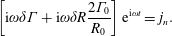 $$\begin{eqnarray}\left[\text{i}\unicode[STIX]{x1D714}\unicode[STIX]{x1D6FF}\unicode[STIX]{x1D6E4}+\text{i}\unicode[STIX]{x1D714}\unicode[STIX]{x1D6FF}R\frac{2\unicode[STIX]{x1D6E4}_{0}}{R_{0}}\right]\text{e}^{\text{i}\unicode[STIX]{x1D714}t}=j_{n}.\end{eqnarray}$$
In systems where the surfactant is insoluble (for which $j_{n}=0$
), the change in surface concentration is
$j_{n}=0$
), the change in surface concentration is
 $$\begin{eqnarray}\unicode[STIX]{x1D6FF}\unicode[STIX]{x1D6E4}_{insol}=-\frac{2\unicode[STIX]{x1D6E4}_{0}}{R_{0}}\unicode[STIX]{x1D6FF}R.\end{eqnarray}$$
We define $C_{s}$
and
$C_{s}$
and $\unicode[STIX]{x1D6FF}C_{s}$
as the bulk concentration and the amplitude of its oscillatory perturbation at the interface
$\unicode[STIX]{x1D6FF}C_{s}$
as the bulk concentration and the amplitude of its oscillatory perturbation at the interface
 $$\begin{eqnarray}C_{s}(t)=C(R,t),\quad \text{and}\quad \unicode[STIX]{x1D6FF}C_{s}=\unicode[STIX]{x1D6FF}C(R).\end{eqnarray}$$
Because the convective term in the bulk transport equation (3.26) is quadratic in perturbed quantities, the bulk concentration $C$
obeys the diffusion equation to leading order, with solution
$C$
obeys the diffusion equation to leading order, with solution
 $$\begin{eqnarray}C(r,t)=C_{0}+\unicode[STIX]{x1D6FF}C_{s}\frac{R}{r}\text{e}^{\sqrt{\text{i}\unicode[STIX]{x1D714}/D}(R-r)}\text{e}^{\text{i}\unicode[STIX]{x1D714}t},\end{eqnarray}$$
where $\unicode[STIX]{x1D6FF}C_{s}$
is as yet unknown. The diffusive flux (3.27) onto the interface,
$\unicode[STIX]{x1D6FF}C_{s}$
is as yet unknown. The diffusive flux (3.27) onto the interface,
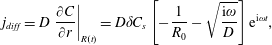 $$\begin{eqnarray}j_{diff}=D\left.\frac{\unicode[STIX]{x2202}C}{\unicode[STIX]{x2202}r}\right|_{R(t)}=D\unicode[STIX]{x1D6FF}C_{s}\left[-\frac{1}{R_{0}}-\sqrt{\frac{\text{i}\unicode[STIX]{x1D714}}{D}}\right]\text{e}^{\text{i}\unicode[STIX]{x1D714}t},\end{eqnarray}$$
must equal the kinetic flux $j_{kin}$
(3.24), which is given to leading order by
$j_{kin}$
(3.24), which is given to leading order by
 $$\begin{eqnarray}j_{kin}=\left(k_{C}\unicode[STIX]{x1D6FF}C_{s}-k_{\unicode[STIX]{x1D6E4}}\unicode[STIX]{x1D6FF}\unicode[STIX]{x1D6E4}\right)\text{e}^{\text{i}\unicode[STIX]{x1D714}t}.\end{eqnarray}$$
Here
 $$\begin{eqnarray}\displaystyle & \displaystyle k_{C}(C_{0},\unicode[STIX]{x1D6E4}_{0})=\left.\frac{\unicode[STIX]{x2202}j_{a}}{\unicode[STIX]{x2202}C}\right|_{\unicode[STIX]{x1D6E4}_{0},C_{0}}-\left.\frac{\unicode[STIX]{x2202}j_{d}}{\unicode[STIX]{x2202}C}\right|_{\unicode[STIX]{x1D6E4}_{0},C_{0}}, & \displaystyle\end{eqnarray}$$
 $$\begin{eqnarray}\displaystyle & \displaystyle k_{\unicode[STIX]{x1D6E4}}(C_{0},\unicode[STIX]{x1D6E4}_{0})=\left.\frac{\unicode[STIX]{x2202}j_{a}}{\unicode[STIX]{x2202}\unicode[STIX]{x1D6E4}}\right|_{\unicode[STIX]{x1D6E4}_{0},C_{0}}-\left.\frac{\unicode[STIX]{x2202}j_{d}}{\unicode[STIX]{x2202}\unicode[STIX]{x1D6E4}}\right|_{\unicode[STIX]{x1D6E4}_{0},C_{0}} & \displaystyle\end{eqnarray}$$ $k_{C}$
and
$k_{C}$
and $k_{\unicode[STIX]{x1D6E4}}$
has units of length and is defined as the depletion depth
$k_{\unicode[STIX]{x1D6E4}}$
has units of length and is defined as the depletion depth  $$\begin{eqnarray}L_{d}=\frac{k_{C}}{k_{\unicode[STIX]{x1D6E4}}}.\end{eqnarray}$$
For example, the (linear) Henry isotherm (table 1) has $k_{C}=k_{a}$
and
$k_{C}=k_{a}$
and $k_{\unicode[STIX]{x1D6E4}}=k_{d}$
, so that the depletion depth is a constant equal to the equilibrium adsorption constant:
$k_{\unicode[STIX]{x1D6E4}}=k_{d}$
, so that the depletion depth is a constant equal to the equilibrium adsorption constant: $L_{d}=K^{ideal}$
.
$L_{d}=K^{ideal}$
.
Equating the diffusive (3.35) and kinetic fluxes (3.36) relates $\unicode[STIX]{x1D6FF}C_{s}$
to
$\unicode[STIX]{x1D6FF}C_{s}$
to $\unicode[STIX]{x1D6FF}\unicode[STIX]{x1D6E4}$
:
$\unicode[STIX]{x1D6FF}\unicode[STIX]{x1D6E4}$
:
 $$\begin{eqnarray}\unicode[STIX]{x1D6FF}C_{s}=\frac{k_{\unicode[STIX]{x1D6E4}}R_{0}}{D+k_{C}R_{0}+\sqrt{\text{i}\unicode[STIX]{x1D714}R_{0}^{2}D}}\unicode[STIX]{x1D6FF}\unicode[STIX]{x1D6E4}=\frac{Da}{1+Da+\sqrt{\text{i}Wo}}\frac{\unicode[STIX]{x1D6FF}\unicode[STIX]{x1D6E4}}{L_{d}},\end{eqnarray}$$
where the mass transfer Womersley number $Wo$
and Damköhler number
$Wo$
and Damköhler number $Da$
are
$Da$
are
 $$\begin{eqnarray}\displaystyle & \displaystyle Wo=\frac{diffusion~time}{oscillation~period}=\frac{\unicode[STIX]{x1D714}R_{0}^{2}}{D}, & \displaystyle\end{eqnarray}$$
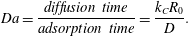 $$\begin{eqnarray}\displaystyle & \displaystyle Da=\frac{diffusion~time}{adsorption~time}=\frac{k_{C}R_{0}}{D}. & \displaystyle\end{eqnarray}$$
Then, using (3.39) in (3.35) or (3.36) to eliminate $\unicode[STIX]{x1D6FF}C_{s}$
and determine
$\unicode[STIX]{x1D6FF}C_{s}$
and determine $j_{n}$
in terms of
$j_{n}$
in terms of $\unicode[STIX]{x1D6FF}\unicode[STIX]{x1D6E4}$
, and substituting into the surface conservation equation (3.31) reveals
$\unicode[STIX]{x1D6FF}\unicode[STIX]{x1D6E4}$
, and substituting into the surface conservation equation (3.31) reveals $\unicode[STIX]{x1D6FF}\unicode[STIX]{x1D6E4}$
to be
$\unicode[STIX]{x1D6FF}\unicode[STIX]{x1D6E4}$
to be
 $$\begin{eqnarray}\frac{\unicode[STIX]{x1D6FF}\unicode[STIX]{x1D6E4}}{\unicode[STIX]{x1D6FF}\unicode[STIX]{x1D6E4}_{insol}}=\left[1-\text{i}\,St\left(\frac{1+\sqrt{\text{i}\,Wo}}{1+\sqrt{\text{i}\,Wo}+Da}\right)\right]^{-1},\end{eqnarray}$$
where the Stanton number $St$
is defined by
$St$
is defined by
 $$\begin{eqnarray}St=\frac{oscillation~period}{desorption~time}=\frac{k_{\unicode[STIX]{x1D6E4}}}{\unicode[STIX]{x1D714}}.\end{eqnarray}$$
The Damköhler number controls the transition from kinetically limited ( $Da\ll 1$
) to diffusion-limited (
$Da\ll 1$
) to diffusion-limited ( $Da\gg 1$
) surfactant exchange. In what follows (§§ 3.2.2–3.2.3), we consider kinetically and diffusion-controlled regimes separately. For later use, we rewrite the surfactant exchange flux, from (3.35) or (3.36), as
$Da\gg 1$
) surfactant exchange. In what follows (§§ 3.2.2–3.2.3), we consider kinetically and diffusion-controlled regimes separately. For later use, we rewrite the surfactant exchange flux, from (3.35) or (3.36), as
 $$\begin{eqnarray}j_{n}=j_{diff}=j_{kin}=-\left[\frac{1+\sqrt{\text{i}\,Wo}}{1+\sqrt{\text{i}\,Wo}+Da}\right]k_{\unicode[STIX]{x1D6E4}}\unicode[STIX]{x1D6FF}\unicode[STIX]{x1D6E4}\text{e}^{\text{i}\unicode[STIX]{x1D714}t}.\end{eqnarray}$$
3.2.2 Kinetically limited mass transfer (
$Da\ll 1$
)

Adsorption is kinetically limited ( $Da\ll 1$
) when molecular exchange between the interface and the subsurface layer is significantly slower than surfactant diffusion through the bulk. In this limit, the subphase concentration is approximately uniform: (3.39) gives
$Da\ll 1$
) when molecular exchange between the interface and the subsurface layer is significantly slower than surfactant diffusion through the bulk. In this limit, the subphase concentration is approximately uniform: (3.39) gives $\unicode[STIX]{x1D6FF}C_{s}\rightarrow 0$
as
$\unicode[STIX]{x1D6FF}C_{s}\rightarrow 0$
as $Da\rightarrow 0$
, implying
$Da\rightarrow 0$
, implying $C_{s}(t)\approx C_{0}$
(figure 7
e).
$C_{s}(t)\approx C_{0}$
(figure 7
e).

Figure 8. (a) Real (solid line) and imaginary (broken line) components of the perturbed surface concentration for kinetically limited adsorption ( $Da\rightarrow 0$
) to an oscillating bubble, from (3.44). (b) Surface concentration in diffusion-limited mass transfer (
$Da\rightarrow 0$
) to an oscillating bubble, from (3.44). (b) Surface concentration in diffusion-limited mass transfer ( $Da\rightarrow \infty$
), from (3.50).
$Da\rightarrow \infty$
), from (3.50). $\unicode[STIX]{x1D6EC}_{d}=0$
represents a planar interface following (3.48). The vertical dashed lines show locations where
$\unicode[STIX]{x1D6EC}_{d}=0$
represents a planar interface following (3.48). The vertical dashed lines show locations where $2\unicode[STIX]{x1D6EC}_{d}\unicode[STIX]{x1D701}_{d}^{2}=1$
when
$2\unicode[STIX]{x1D6EC}_{d}\unicode[STIX]{x1D701}_{d}^{2}=1$
when $\unicode[STIX]{x1D6EC}_{d}\gtrsim 1$
, indicating modified diffusion times for small bubbles via (3.53).
$\unicode[STIX]{x1D6EC}_{d}\gtrsim 1$
, indicating modified diffusion times for small bubbles via (3.53).
Setting $Da=0$
in (3.41) gives the perturbed surface concentration
$Da=0$
in (3.41) gives the perturbed surface concentration
 $$\begin{eqnarray}\frac{\unicode[STIX]{x1D6FF}\unicode[STIX]{x1D6E4}_{kin}}{\unicode[STIX]{x1D6FF}\unicode[STIX]{x1D6E4}_{insol}}=\frac{1}{1-\text{i}\,St}=\frac{1}{1+St^{2}}+\text{i}\frac{St}{1+St^{2}}.\end{eqnarray}$$
The $St\rightarrow 0$
limit corresponds to oscillations so rapid that surfactants do not have the times to adsorb or desorb, so that the monolayer behaves as if it were insoluble:
$St\rightarrow 0$
limit corresponds to oscillations so rapid that surfactants do not have the times to adsorb or desorb, so that the monolayer behaves as if it were insoluble: $\unicode[STIX]{x1D6FF}\unicode[STIX]{x1D6E4}_{kin}\rightarrow \unicode[STIX]{x1D6FF}\unicode[STIX]{x1D6E4}_{insol}$
. By contrast, the
$\unicode[STIX]{x1D6FF}\unicode[STIX]{x1D6E4}_{kin}\rightarrow \unicode[STIX]{x1D6FF}\unicode[STIX]{x1D6E4}_{insol}$
. By contrast, the $St\rightarrow \infty$
limit occurs when surfactants adsorb/desorb much faster than bubble oscillations. In that case,
$St\rightarrow \infty$
limit occurs when surfactants adsorb/desorb much faster than bubble oscillations. In that case, $\unicode[STIX]{x1D6FF}\unicode[STIX]{x1D6E4}_{kin}\rightarrow 0$
and the interface maintains its equilibrium concentration
$\unicode[STIX]{x1D6FF}\unicode[STIX]{x1D6E4}_{kin}\rightarrow 0$
and the interface maintains its equilibrium concentration $\unicode[STIX]{x1D6E4}(t)\approx \unicode[STIX]{x1D6E4}_{0}$
.
$\unicode[STIX]{x1D6E4}(t)\approx \unicode[STIX]{x1D6E4}_{0}$
.
Time scales for bubble oscillation and adsorption/desorption are comparable when $St\sim O(1)$
, which defines the characteristic time scale for kinetically limited adsorption:
$St\sim O(1)$
, which defines the characteristic time scale for kinetically limited adsorption:
 $$\begin{eqnarray}\unicode[STIX]{x1D70F}_{k}=\frac{1}{k_{\unicode[STIX]{x1D6E4}}}.\end{eqnarray}$$
For finite $\unicode[STIX]{x1D70F}_{k}$
(or finite
$\unicode[STIX]{x1D70F}_{k}$
(or finite $St$
),
$St$
), $\unicode[STIX]{x1D6FF}\unicode[STIX]{x1D6E4}_{kin}$
is always smaller than
$\unicode[STIX]{x1D6FF}\unicode[STIX]{x1D6E4}_{kin}$
is always smaller than $\unicode[STIX]{x1D6FF}\unicode[STIX]{x1D6E4}_{insol}$
(figure 8
a). Additionally, the surface concentration lags the bubble radius by a phase shift
$\unicode[STIX]{x1D6FF}\unicode[STIX]{x1D6E4}_{insol}$
(figure 8
a). Additionally, the surface concentration lags the bubble radius by a phase shift $\tan ^{-1}(St)$
.
$\tan ^{-1}(St)$
.
When kinetically limited ( $Da\rightarrow 0$
), the adsorption flux (3.43) becomes
$Da\rightarrow 0$
), the adsorption flux (3.43) becomes
 $$\begin{eqnarray}j_{n}(Da\rightarrow 0)=-k_{\unicode[STIX]{x1D6E4}}\unicode[STIX]{x1D6FF}\unicode[STIX]{x1D6E4}\text{e}^{\text{i}\unicode[STIX]{x1D714}t}=\frac{\unicode[STIX]{x1D6E4}_{0}-\unicode[STIX]{x1D6E4}(t)}{\unicode[STIX]{x1D70F}_{k}}.\end{eqnarray}$$
Throughout this work, we will use (3.46) as the kinetically limited sorptive flux for small departures from equilibrium.
3.2.3 Diffusion-limited mass transfer (
$Da\gg 1$
)

In diffusion-controlled surfactant exchange, adsorption kinetics are so fast that $\unicode[STIX]{x1D6E4}$
equilibrates with the subsurface concentration
$\unicode[STIX]{x1D6E4}$
equilibrates with the subsurface concentration $C_{s}$
effectively instantaneously, via the appropriate isotherm
$C_{s}$
effectively instantaneously, via the appropriate isotherm $\unicode[STIX]{x1D6E4}(C_{s})$
(figure 7
d). In this limit,
$\unicode[STIX]{x1D6E4}(C_{s})$
(figure 7
d). In this limit, $j_{kin}$
can be ignored, so that
$j_{kin}$
can be ignored, so that $j_{n}=j_{diff}$
. The depletion depth
$j_{n}=j_{diff}$
. The depletion depth $L_{d}$
follows by expanding
$L_{d}$
follows by expanding $\unicode[STIX]{x1D6E4}(C_{s})$
around
$\unicode[STIX]{x1D6E4}(C_{s})$
around $\unicode[STIX]{x1D6E4}_{0}(C_{0})$
, and taking the
$\unicode[STIX]{x1D6E4}_{0}(C_{0})$
, and taking the $Da\rightarrow \infty$
limit of (3.39) to give
$Da\rightarrow \infty$
limit of (3.39) to give
 $$\begin{eqnarray}\left.\frac{\unicode[STIX]{x2202}\unicode[STIX]{x1D6E4}}{\unicode[STIX]{x2202}C_{s}}\right|_{\unicode[STIX]{x1D6E4}_{0},C_{0}}=\left.\frac{\unicode[STIX]{x1D6FF}\unicode[STIX]{x1D6E4}}{\unicode[STIX]{x1D6FF}C_{s}}\right|_{Da\rightarrow \infty }=L_{d},\end{eqnarray}$$
which we non-dimensionalize by the bubble radius $R_{0}$
to give
$R_{0}$
to give
 $$\begin{eqnarray}\unicode[STIX]{x1D6EC}_{d}=\frac{L_{d}}{R_{0}}=\frac{Da}{St\,Wo}.\end{eqnarray}$$
The perturbed surface concentration (3.41) in the diffusion-controlled limit ( $Da\rightarrow \infty$
) is then
$Da\rightarrow \infty$
) is then
 $$\begin{eqnarray}\frac{\unicode[STIX]{x1D6FF}\unicode[STIX]{x1D6E4}_{diff}}{\unicode[STIX]{x1D6FF}\unicode[STIX]{x1D6E4}_{insol}}=\frac{\unicode[STIX]{x1D6EC}_{d}Wo}{\unicode[STIX]{x1D6EC}_{d}Wo-\text{i}-\text{i}\sqrt{\text{i}\,Wo}},\end{eqnarray}$$
which can be expressed as
 $$\begin{eqnarray}\frac{\unicode[STIX]{x1D6FF}\unicode[STIX]{x1D6E4}_{diff}}{\unicode[STIX]{x1D6FF}\unicode[STIX]{x1D6E4}_{insol}}=\frac{1+\unicode[STIX]{x1D701}_{d}+\text{i}\unicode[STIX]{x1D701}_{d}(1+2\unicode[STIX]{x1D6EC}_{d}\unicode[STIX]{x1D701}_{d})}{1+2\unicode[STIX]{x1D701}_{d}+2\unicode[STIX]{x1D701}_{d}^{2}(1+2\unicode[STIX]{x1D6EC}_{d}\unicode[STIX]{x1D701}_{d}+2\unicode[STIX]{x1D6EC}_{d}^{2}\unicode[STIX]{x1D701}_{d}^{2})},\end{eqnarray}$$
where
 $$\begin{eqnarray}\unicode[STIX]{x1D701}_{d}=\frac{1}{\unicode[STIX]{x1D6EC}_{d}}\sqrt{\frac{1}{2Wo}}=\frac{1}{L_{d}}\sqrt{\frac{D}{2\unicode[STIX]{x1D714}}}\end{eqnarray}$$
is a dimensionless ratio of the diffusive oscillatory boundary layer thickness $\unicode[STIX]{x1D6FF}_{BL}=\sqrt{D/2\unicode[STIX]{x1D714}}$
to the depletion depth
$\unicode[STIX]{x1D6FF}_{BL}=\sqrt{D/2\unicode[STIX]{x1D714}}$
to the depletion depth $L_{d}$
.
$L_{d}$
.
Bubbles with radii much larger than the depletion depth ( $\unicode[STIX]{x1D6EC}_{d}\ll 1$
) behave like planar interfaces. Indeed, (3.50) recovers the celebrated results of Lucassen & van den Tempel (Reference Lucassen and van den Tempel1972) in the
$\unicode[STIX]{x1D6EC}_{d}\ll 1$
) behave like planar interfaces. Indeed, (3.50) recovers the celebrated results of Lucassen & van den Tempel (Reference Lucassen and van den Tempel1972) in the $\unicode[STIX]{x1D6EC}_{d}\rightarrow 0$
limit, which we examine in detail in § 4.2.1. Adsorbed surfactants on a planar interface (
$\unicode[STIX]{x1D6EC}_{d}\rightarrow 0$
limit, which we examine in detail in § 4.2.1. Adsorbed surfactants on a planar interface ( $\unicode[STIX]{x1D6EC}_{d}\rightarrow 0$
) act as effectively insoluble if molecules in the subphase diffuse far less than the depletion depth in one oscillation (
$\unicode[STIX]{x1D6EC}_{d}\rightarrow 0$
) act as effectively insoluble if molecules in the subphase diffuse far less than the depletion depth in one oscillation ( $\unicode[STIX]{x1D701}_{d}\ll 1$
). Conversely, the surface concentration remains close to its equilibrium value (
$\unicode[STIX]{x1D701}_{d}\ll 1$
). Conversely, the surface concentration remains close to its equilibrium value ( $\unicode[STIX]{x1D6FF}\unicode[STIX]{x1D6E4}_{diff}\rightarrow 0$
) if molecules diffusively escape
$\unicode[STIX]{x1D6FF}\unicode[STIX]{x1D6E4}_{diff}\rightarrow 0$
) if molecules diffusively escape $L_{d}$
during an oscillation (
$L_{d}$
during an oscillation ( $\unicode[STIX]{x1D701}_{d}\gg 1$
). Interfacial oscillations and diffusive mass transfer are comparable when
$\unicode[STIX]{x1D701}_{d}\gg 1$
). Interfacial oscillations and diffusive mass transfer are comparable when $\unicode[STIX]{x1D701}_{d}=O(1)$
, which reveals the characteristic time scale for diffusion-limited mass transfer in the planar limit (
$\unicode[STIX]{x1D701}_{d}=O(1)$
, which reveals the characteristic time scale for diffusion-limited mass transfer in the planar limit ( $\unicode[STIX]{x1D6EC}_{d}\rightarrow 0$
) to be
$\unicode[STIX]{x1D6EC}_{d}\rightarrow 0$
) to be
 $$\begin{eqnarray}\unicode[STIX]{x1D70F}_{d,p}=\unicode[STIX]{x1D70F}_{d}(\unicode[STIX]{x1D6EC}_{d}\rightarrow 0)=\frac{L_{d}^{2}}{D}.\end{eqnarray}$$
Diffusive mass transfer is sensitive to interfacial curvature when $\unicode[STIX]{x1D6EC}_{d}\gtrsim 1$
, as shown in figure 8(b). The perturbed surface concentration
$\unicode[STIX]{x1D6EC}_{d}\gtrsim 1$
, as shown in figure 8(b). The perturbed surface concentration $\unicode[STIX]{x1D6FF}\unicode[STIX]{x1D6E4}_{diff}$
still vanishes if diffusion is fast (
$\unicode[STIX]{x1D6FF}\unicode[STIX]{x1D6E4}_{diff}$
still vanishes if diffusion is fast ( $\unicode[STIX]{x1D701}_{d}\gg 1$
) and approaches the insoluble limit if diffusion is slow (
$\unicode[STIX]{x1D701}_{d}\gg 1$
) and approaches the insoluble limit if diffusion is slow ( $\unicode[STIX]{x1D701}_{d}\ll 1$
). However, the transition occurs around
$\unicode[STIX]{x1D701}_{d}\ll 1$
). However, the transition occurs around $\unicode[STIX]{x1D6EC}_{d}\unicode[STIX]{x1D701}_{d}^{2}=O(1)$
, where
$\unicode[STIX]{x1D6EC}_{d}\unicode[STIX]{x1D701}_{d}^{2}=O(1)$
, where
 $$\begin{eqnarray}2\unicode[STIX]{x1D6EC}_{d}\unicode[STIX]{x1D701}_{d}^{2}=\frac{D/L_{d}R_{0}}{\unicode[STIX]{x1D714}}\sim \frac{oscillation~period}{diffusion~time~across~\sqrt{L_{d}R_{0}}},\end{eqnarray}$$
which reveals the characteristic time scale of diffusive-controlled surfactant exchange for small bubbles ( $\unicode[STIX]{x1D6EC}_{d}\gtrsim 1$
)
$\unicode[STIX]{x1D6EC}_{d}\gtrsim 1$
)
 $$\begin{eqnarray}\unicode[STIX]{x1D70F}_{d,s}=\unicode[STIX]{x1D70F}_{d}(\unicode[STIX]{x1D6EC}_{d}\gtrsim 1)=\frac{L_{d}R_{0}}{D}=\frac{\unicode[STIX]{x1D70F}_{d,p}}{\unicode[STIX]{x1D6EC}_{d}}.\end{eqnarray}$$
Indeed, experiments and simulations show a smooth transition from $\unicode[STIX]{x1D70F}_{d,p}$
to
$\unicode[STIX]{x1D70F}_{d,p}$
to $\unicode[STIX]{x1D70F}_{d,s}$
with decreasing bubble radius (Alvarez, Walker & Anna Reference Alvarez, Walker and Anna2010a
,Reference Alvarez, Walker and Anna
b
).
$\unicode[STIX]{x1D70F}_{d,s}$
with decreasing bubble radius (Alvarez, Walker & Anna Reference Alvarez, Walker and Anna2010a
,Reference Alvarez, Walker and Anna
b
).
Finally, the diffusion-limited surfactant exchange flux follows from the $Da\rightarrow \infty$
limit of (3.43). For small bubbles (
$Da\rightarrow \infty$
limit of (3.43). For small bubbles ( $R_{0}^{2}\ll D/\unicode[STIX]{x1D714}$
, or
$R_{0}^{2}\ll D/\unicode[STIX]{x1D714}$
, or $Wo\,\ll 1$
), the net adsorption flux is
$Wo\,\ll 1$
), the net adsorption flux is
 $$\begin{eqnarray}j_{n}(Da\rightarrow \infty )\approx -\frac{k_{\unicode[STIX]{x1D6E4}}}{Da}\unicode[STIX]{x1D6FF}\unicode[STIX]{x1D6E4}\text{e}^{\text{i}\unicode[STIX]{x1D714}t}=-\frac{D}{L_{d}R_{0}}\unicode[STIX]{x1D6FF}\unicode[STIX]{x1D6E4}\text{e}^{\text{i}\unicode[STIX]{x1D714}t}=\frac{\unicode[STIX]{x1D6E4}_{0}-\unicode[STIX]{x1D6E4}(t)}{\unicode[STIX]{x1D70F}_{d,s}},\end{eqnarray}$$
which has the same form as (3.46), but with the diffusion-controlled time scale $\unicode[STIX]{x1D70F}_{d,s}$
in place of the kinetically controlled time scale
$\unicode[STIX]{x1D70F}_{d,s}$
in place of the kinetically controlled time scale $\unicode[STIX]{x1D70F}_{k}$
. For the same reasons,
$\unicode[STIX]{x1D70F}_{k}$
. For the same reasons, $\unicode[STIX]{x1D6FF}\unicode[STIX]{x1D6E4}_{diff}(\unicode[STIX]{x1D6EC}_{d}\gg 1)$
from (3.50) is identical to
$\unicode[STIX]{x1D6FF}\unicode[STIX]{x1D6E4}_{diff}(\unicode[STIX]{x1D6EC}_{d}\gg 1)$
from (3.50) is identical to $\unicode[STIX]{x1D6FF}\unicode[STIX]{x1D6E4}_{kin}$
from (3.44) with
$\unicode[STIX]{x1D6FF}\unicode[STIX]{x1D6E4}_{kin}$
from (3.44) with $2\unicode[STIX]{x1D6EC}_{d}\unicode[STIX]{x1D701}_{d}^{2}$
in place of
$2\unicode[STIX]{x1D6EC}_{d}\unicode[STIX]{x1D701}_{d}^{2}$
in place of $St$
. In other words, diffusion-limited mass transfer to small bubbles ‘looks like’ it is kinetically limited, albeit with a characteristic time scale
$St$
. In other words, diffusion-limited mass transfer to small bubbles ‘looks like’ it is kinetically limited, albeit with a characteristic time scale $\unicode[STIX]{x1D70F}_{d,s}$
that depends on the bubble radius via (3.54).
$\unicode[STIX]{x1D70F}_{d,s}$
that depends on the bubble radius via (3.54).
To summarize, the characteristic sorption time $\unicode[STIX]{x1D70F}_{s}$
is
$\unicode[STIX]{x1D70F}_{s}$
is
 $$\begin{eqnarray}\unicode[STIX]{x1D70F}_{s}=\left\{\begin{array}{@{}ll@{}}\unicode[STIX]{x1D70F}_{k}=1/k_{\unicode[STIX]{x1D6E4}},\quad & Da\ll 1,\\ \unicode[STIX]{x1D70F}_{d,p}=L_{d}^{2}/D,\quad & Da\gg 1\text{ and }R_{0}\gg L_{d},\\ \unicode[STIX]{x1D70F}_{d,s}=L_{d}R_{0}/D,\quad & Da\gg 1\text{ and }R_{0}\lesssim L_{d}.\end{array}\right.\end{eqnarray}$$
In systems with dynamic interfaces, the mechanical response of a surface to deformation depends not only on the equilibrium properties of the surfactant (such as $E_{0}$
, § 2.3.1), but also on the adsorbed concentration profile
$E_{0}$
, § 2.3.1), but also on the adsorbed concentration profile $\unicode[STIX]{x1D6E4}(\boldsymbol{r}_{s},t)$
at any particular position and time. In § 4.2, we will again use the oscillating gas bubble example to quantify the apparent viscoelasticity of soluble monolayers, and its dependence on surfactant properties such as
$\unicode[STIX]{x1D6E4}(\boldsymbol{r}_{s},t)$
at any particular position and time. In § 4.2, we will again use the oscillating gas bubble example to quantify the apparent viscoelasticity of soluble monolayers, and its dependence on surfactant properties such as $k_{\unicode[STIX]{x1D6E4}}$
,
$k_{\unicode[STIX]{x1D6E4}}$
, $k_{C}$
,
$k_{C}$
, $D$
and
$D$
and $E_{0}$
.
$E_{0}$
.
3.2.4 Adsorption to a clean interface
So far, we have discussed surfactant transport on interfaces that are perturbed only slightly from equilibrium. Ward & Tordai (Reference Ward and Tordai1946) pursued a complementary problem: the diffusion-limited mass transfer to an initially clean planar interface. More recently, Jin, Balasubramaniam & Stebe (Reference Jin, Balasubramaniam and Stebe2004) and Alvarez et al. (Reference Alvarez, Walker and Anna2010a ,Reference Alvarez, Walker and Anna b ) established the critical role of interfacial curvature on surfactant transport. In what follows, we explore their calculations of surfactant exchange to an initially clean static bubble, in both diffusion- and kinetically limited regimes.
The system is the same as in § 3.2.1, except that the bubble interface is stationary, $R(t)=R_{0}$
, and is initially clean:
$R(t)=R_{0}$
, and is initially clean: $\unicode[STIX]{x1D6E4}(0)=0$
. Surfactant is dissolved in the bulk at concentration
$\unicode[STIX]{x1D6E4}(0)=0$
. Surfactant is dissolved in the bulk at concentration $C_{0}$
, and the subsurface concentration is
$C_{0}$
, and the subsurface concentration is $C(R,t)=C_{s}(t)$
. The surface conservation equation (3.10) with the diffusive flux
$C(R,t)=C_{s}(t)$
. The surface conservation equation (3.10) with the diffusive flux $j_{diff}$
from the bulk is
$j_{diff}$
from the bulk is
 $$\begin{eqnarray}\frac{\unicode[STIX]{x2202}\unicode[STIX]{x1D6E4}}{\unicode[STIX]{x2202}t}=D\left.\frac{\unicode[STIX]{x2202}C}{\unicode[STIX]{x2202}r}\right|_{r=R},\end{eqnarray}$$
where $C(R,t)$
follows from the solution of the bulk diffusion equation. Laplace transforming (3.57), denoted by tildes, gives
$C(R,t)$
follows from the solution of the bulk diffusion equation. Laplace transforming (3.57), denoted by tildes, gives
 $$\begin{eqnarray}s\tilde{\unicode[STIX]{x1D6E4}}=D\left.\frac{\unicode[STIX]{x2202}\tilde{C}}{\unicode[STIX]{x2202}r}\right|_{r=R},\end{eqnarray}$$
where $s$
is the Laplace transform variable. Laplace transforming the bulk diffusion equation gives
$s$
is the Laplace transform variable. Laplace transforming the bulk diffusion equation gives
 $$\begin{eqnarray}s\tilde{C}-C_{0}=D\unicode[STIX]{x1D6FB}^{2}\tilde{C},\end{eqnarray}$$
with solution
 $$\begin{eqnarray}\tilde{C}(r,s)=\frac{C_{0}}{s}+\frac{C_{1}}{r}\text{e}^{-r\sqrt{s/D}},\end{eqnarray}$$
where $C_{1}$
is as yet unknown. Evaluating (3.58) with (3.60), then eliminating
$C_{1}$
is as yet unknown. Evaluating (3.58) with (3.60), then eliminating $C_{1}$
in (3.60) in favour of
$C_{1}$
in (3.60) in favour of $C_{s}$
gives
$C_{s}$
gives
 $$\begin{eqnarray}\tilde{\unicode[STIX]{x1D6E4}}(s)=\sqrt{D}\left[\frac{C_{0}}{s^{3/2}}-\frac{\tilde{C}_{s}(s)}{\sqrt{s}}\right]+\frac{D}{R}\left[\frac{C_{0}}{s^{2}}-\frac{\tilde{C}_{s}(s)}{s}\right].\end{eqnarray}$$
Finally, inverting the Laplace transform of (3.61) gives
 $$\begin{eqnarray}\unicode[STIX]{x1D6E4}(t)=\sqrt{\frac{D}{\unicode[STIX]{x03C0}}}\left[2C_{0}\sqrt{t}-\int _{0}^{t}\frac{C_{s}(t^{\prime })}{\sqrt{t-t^{\prime }}}\,\text{d}t^{\prime }\right]+\frac{D}{R}\left[C_{0}t-\int _{0}^{t}C_{s}(t^{\prime })\,\text{d}t^{\prime }\right].\end{eqnarray}$$
The first term on the right-hand side reflects the solution of Ward & Tordai (Reference Ward and Tordai1946) for adsorption onto a clean planar interface, whereas the last two terms reflect interfacial curvature (Jin et al. Reference Jin, Balasubramaniam and Stebe2004; Alvarez et al. Reference Alvarez, Walker and Anna2010a ).
The generalized Ward–Tordai result (3.62) is an implicit integral relation between $\unicode[STIX]{x1D6E4}(t)$
and the yet undetermined subsurface concentration
$\unicode[STIX]{x1D6E4}(t)$
and the yet undetermined subsurface concentration $C_{s}(t)$
. Solving for the surface concentration requires another relationship between
$C_{s}(t)$
. Solving for the surface concentration requires another relationship between $\unicode[STIX]{x1D6E4}(t)$
and
$\unicode[STIX]{x1D6E4}(t)$
and $C_{s}(t)$
, which follows from the kinetic flux condition (3.24). However, inverting this relation is not straightforward except for the simplest kinetic flux expressions, and is typically solved numerically (Jin et al.
Reference Jin, Balasubramaniam and Stebe2004; Alvarez et al.
Reference Alvarez, Walker and Anna2010a
). For example, the 2-D ideal gas assumption (table 2) gives
$C_{s}(t)$
, which follows from the kinetic flux condition (3.24). However, inverting this relation is not straightforward except for the simplest kinetic flux expressions, and is typically solved numerically (Jin et al.
Reference Jin, Balasubramaniam and Stebe2004; Alvarez et al.
Reference Alvarez, Walker and Anna2010a
). For example, the 2-D ideal gas assumption (table 2) gives
 $$\begin{eqnarray}\frac{\unicode[STIX]{x2202}\unicode[STIX]{x1D6E4}}{\unicode[STIX]{x2202}t}=k_{a}C_{s}-k_{d}\unicode[STIX]{x1D6E4},\end{eqnarray}$$
with Laplace transform
 $$\begin{eqnarray}s\tilde{\unicode[STIX]{x1D6E4}}=k_{a}\tilde{C}_{s}-k_{d}\tilde{\unicode[STIX]{x1D6E4}}.\end{eqnarray}$$
In principle, eliminating $\tilde{C}_{s}$
between (3.64) and (3.61), and inverse Laplace transforming
$\tilde{C}_{s}$
between (3.64) and (3.61), and inverse Laplace transforming $\tilde{\unicode[STIX]{x1D6E4}}(s)$
gives an explicit expression for
$\tilde{\unicode[STIX]{x1D6E4}}(s)$
gives an explicit expression for $\unicode[STIX]{x1D6E4}(t)$
. In fact, Hansen (Reference Hansen1961) employs this strategy to examine adsorption to a planar interface (
$\unicode[STIX]{x1D6E4}(t)$
. In fact, Hansen (Reference Hansen1961) employs this strategy to examine adsorption to a planar interface ( $R\rightarrow \infty$
).
$R\rightarrow \infty$
).
Even for the simplest kinetic flux (3.63), however, adsorption to a spherical interface is intractable at arbitrary Damköhler number. Instead, we highlight the kinetically controlled ( $Da\ll 1$
) and diffusion-controlled (
$Da\ll 1$
) and diffusion-controlled ( $Da\gg 1$
) limits individually, by ignoring
$Da\gg 1$
) limits individually, by ignoring $j_{diff}$
and
$j_{diff}$
and $j_{kin}$
, respectively. These limits are easier to calculate, and are illustrative in light of the discussion around oscillating bubbles in the previous section. For later use, we note that the equilibrium surface concentration following (3.63) is
$j_{kin}$
, respectively. These limits are easier to calculate, and are illustrative in light of the discussion around oscillating bubbles in the previous section. For later use, we note that the equilibrium surface concentration following (3.63) is
 $$\begin{eqnarray}\unicode[STIX]{x1D6E4}_{eq}=L_{d}C_{0},\end{eqnarray}$$
with depletion depth
 $$\begin{eqnarray}L_{d}=\frac{k_{a}}{k_{d}}=K^{ideal}.\end{eqnarray}$$
When surfactant transport is kinetically limited, diffusion in the bulk is assumed to be instantaneous, so that $C_{s}(t)=C_{0}$
. Laplace transforming (3.63) with
$C_{s}(t)=C_{0}$
. Laplace transforming (3.63) with $C_{s}=C_{0}$
and using (3.65) gives
$C_{s}=C_{0}$
and using (3.65) gives
 $$\begin{eqnarray}\frac{\tilde{\unicode[STIX]{x1D6E4}}_{kin}(s)}{\unicode[STIX]{x1D6E4}_{eq}}=\frac{k_{d}}{s(s+k_{d})},\end{eqnarray}$$
with inverse
 $$\begin{eqnarray}\frac{\unicode[STIX]{x1D6E4}_{kin}(t)}{\unicode[STIX]{x1D6E4}_{eq}}=1-\text{e}^{-k_{d}t},\end{eqnarray}$$
which recovers the kinetically limited sorption time $\unicode[STIX]{x1D70F}_{k}=1/k_{d}$
(3.45). At short times,
$\unicode[STIX]{x1D70F}_{k}=1/k_{d}$
(3.45). At short times, $\unicode[STIX]{x1D6E4}_{kin}$
grows linearly with time, whereas
$\unicode[STIX]{x1D6E4}_{kin}$
grows linearly with time, whereas $\unicode[STIX]{x1D6E4}_{kin}$
approaches
$\unicode[STIX]{x1D6E4}_{kin}$
approaches $\unicode[STIX]{x1D6E4}_{eq}$
exponentially for
$\unicode[STIX]{x1D6E4}_{eq}$
exponentially for $t\gg \unicode[STIX]{x1D70F}_{k}$
(figure 9
a). As with adsorption to an oscillating bubble, kinetically limited mass transfer is independent of bubble size.
$t\gg \unicode[STIX]{x1D70F}_{k}$
(figure 9
a). As with adsorption to an oscillating bubble, kinetically limited mass transfer is independent of bubble size.

Figure 9. (a) Kinetically controlled adsorption (3.68) to an initially clean spherical surface. (b) Diffusion-controlled adsorption (3.71) to a spherical surface. Adsorption occurs over a faster time scale $\unicode[STIX]{x1D70F}_{d,s}$
in smaller bubbles (
$\unicode[STIX]{x1D70F}_{d,s}$
in smaller bubbles ( $\unicode[STIX]{x1D6EC}_{d}=L_{d}/R\gtrsim 1$
), and approaches equilibrium exponentially, rather than as
$\unicode[STIX]{x1D6EC}_{d}=L_{d}/R\gtrsim 1$
), and approaches equilibrium exponentially, rather than as $1/\sqrt{t}$
in the case of large bubbles (
$1/\sqrt{t}$
in the case of large bubbles ( $\unicode[STIX]{x1D6EC}_{d}\rightarrow 0$
).
$\unicode[STIX]{x1D6EC}_{d}\rightarrow 0$
).
By contrast, contact equilibrium is assumed between $\unicode[STIX]{x1D6E4}(t)$
and
$\unicode[STIX]{x1D6E4}(t)$
and $C_{s}(t)$
when adsorption is diffusion controlled, so that
$C_{s}(t)$
when adsorption is diffusion controlled, so that
 $$\begin{eqnarray}\unicode[STIX]{x1D6E4}_{diff}(t)=L_{d}C_{s}(t).\end{eqnarray}$$
Using the Laplace transform of (3.69) to eliminate $\tilde{C}_{s}$
in (3.61) gives
$\tilde{C}_{s}$
in (3.61) gives
 $$\begin{eqnarray}\frac{\tilde{\unicode[STIX]{x1D6E4}}_{diff}(s)}{\unicode[STIX]{x1D6E4}_{eq}}=\frac{s^{1/2}+\sqrt{D/R^{2}}}{s^{3/2}+s\sqrt{D/R^{2}}+s^{2}\sqrt{L_{d}^{2}/D}}.\end{eqnarray}$$
Inverting (3.70) is laborious but straightforward, and yields
 $$\begin{eqnarray}\frac{\unicode[STIX]{x1D6E4}_{diff}(t)}{\unicode[STIX]{x1D6E4}_{eq}}=1+\frac{1}{\unicode[STIX]{x1D6FD}-\unicode[STIX]{x1D6FC}}\left[\unicode[STIX]{x1D6FC}\text{e}^{\unicode[STIX]{x1D6FC}^{2}t}\,\text{erfc}(\unicode[STIX]{x1D6FC}\sqrt{t})-\unicode[STIX]{x1D6FD}\text{e}^{\unicode[STIX]{x1D6FD}^{2}t}\,\text{erfc}(\unicode[STIX]{x1D6FD}\sqrt{t})\right],\end{eqnarray}$$
where
 $$\begin{eqnarray}\unicode[STIX]{x1D6FC}=\frac{\sqrt{D}}{2L_{d}}\left(1+\sqrt{1-4\unicode[STIX]{x1D6EC}_{d}}\right),\quad \unicode[STIX]{x1D6FD}=\frac{\sqrt{D}}{2L_{d}}\left(1-\sqrt{1-4\unicode[STIX]{x1D6EC}_{d}}\right),\end{eqnarray}$$
and $\unicode[STIX]{x1D6EC}_{d}=L_{d}/R$
(3.48).
$\unicode[STIX]{x1D6EC}_{d}=L_{d}/R$
(3.48).
The large- and small-bubble limits of (3.70) are particularly illustrative. Bubbles with radii much larger than the depletion depth ( $\unicode[STIX]{x1D6EC}_{d}\rightarrow 0$
) have
$\unicode[STIX]{x1D6EC}_{d}\rightarrow 0$
) have
 $$\begin{eqnarray}\left.\frac{\unicode[STIX]{x1D6E4}_{diff}(t)}{\unicode[STIX]{x1D6E4}_{eq}}\right|_{\unicode[STIX]{x1D6EC}_{d}\rightarrow 0}=1-\text{e}^{Dt/L_{d}^{2}}\,\text{erfc}(\sqrt{Dt}/L_{d}),\end{eqnarray}$$
recovering the result of Hansen (Reference Hansen1961) for a planar interface. Indeed, the characteristic diffusion time in (3.73) is $\unicode[STIX]{x1D70F}_{d,p}=L_{d}^{2}/D$
, like in diffusion-limited adsorption to large oscillating bubbles (3.52).
$\unicode[STIX]{x1D70F}_{d,p}=L_{d}^{2}/D$
, like in diffusion-limited adsorption to large oscillating bubbles (3.52). $\unicode[STIX]{x1D6E4}_{diff}$
approaches
$\unicode[STIX]{x1D6E4}_{diff}$
approaches $\unicode[STIX]{x1D6E4}_{eq}$
algebraically at long times (figure 9
b), much more slowly than the exponential approach during kinetically controlled adsorption (3.68).
$\unicode[STIX]{x1D6E4}_{eq}$
algebraically at long times (figure 9
b), much more slowly than the exponential approach during kinetically controlled adsorption (3.68).
When the bubble is much smaller than the depletion depth ( $\unicode[STIX]{x1D6EC}_{d}\gg 1$
), however, surface concentration approaches equilibrium exponentially, via
$\unicode[STIX]{x1D6EC}_{d}\gg 1$
), however, surface concentration approaches equilibrium exponentially, via
 $$\begin{eqnarray}\left.\frac{\unicode[STIX]{x1D6E4}_{diff}(t)}{\unicode[STIX]{x1D6E4}_{eq}}\right|_{\unicode[STIX]{x1D6EC}_{d}\gg 1}=1-\text{e}^{-Dt/L_{d}R}.\end{eqnarray}$$
The characteristic diffusion time $\unicode[STIX]{x1D70F}_{d,s}=L_{d}R/D$
that emerges is the same (3.54) that controls small, oscillatory bubbles. As with oscillating bubbles, diffusion-limited adsorption to small bubbles (
$\unicode[STIX]{x1D70F}_{d,s}=L_{d}R/D$
that emerges is the same (3.54) that controls small, oscillatory bubbles. As with oscillating bubbles, diffusion-limited adsorption to small bubbles ( $R\ll L_{d}$
) has the same form as kinetically limited adsorption (3.68), except with
$R\ll L_{d}$
) has the same form as kinetically limited adsorption (3.68), except with $\unicode[STIX]{x1D70F}_{d,s}$
replacing
$\unicode[STIX]{x1D70F}_{d,s}$
replacing $\unicode[STIX]{x1D70F}_{k}$
. As shown in figure 9(b), diffusion-limited adsorption is faster for smaller bubbles, and
$\unicode[STIX]{x1D70F}_{k}$
. As shown in figure 9(b), diffusion-limited adsorption is faster for smaller bubbles, and $\unicode[STIX]{x1D6E4}_{diff}$
approaches
$\unicode[STIX]{x1D6E4}_{diff}$
approaches $\unicode[STIX]{x1D6E4}_{eq}$
exponentially rather than algebraically over long times.
$\unicode[STIX]{x1D6E4}_{eq}$
exponentially rather than algebraically over long times.
Finally, convection in the bulk fluid further enhances the rate of diffusive adsorption by ‘screening’ the characteristic diffusion length by the thickness of the diffusion boundary layer $\unicode[STIX]{x1D6FF}_{BL}$
. Alvarez et al. (Reference Alvarez, Vogus, Walker and Anna2012) demonstrated that the diffusion time is indeed
$\unicode[STIX]{x1D6FF}_{BL}$
. Alvarez et al. (Reference Alvarez, Vogus, Walker and Anna2012) demonstrated that the diffusion time is indeed $\unicode[STIX]{x1D70F}_{d,p}^{conv}\propto \unicode[STIX]{x1D6FF}_{BL}^{2}$
for large bubbles, and
$\unicode[STIX]{x1D70F}_{d,p}^{conv}\propto \unicode[STIX]{x1D6FF}_{BL}^{2}$
for large bubbles, and $\unicode[STIX]{x1D70F}_{d,s}^{conv}\propto \unicode[STIX]{x1D6FF}_{BL}$
for smaller bubbles. This scaling suggests strategies to further speed up diffusive surfactant transport using flow, as the boundary layer thickness decreases with increasing bulk convection, thereby increasing the range of measurable kinetic-limited adsorption (Alvarez et al.
Reference Alvarez, Vogus, Walker and Anna2012).
$\unicode[STIX]{x1D70F}_{d,s}^{conv}\propto \unicode[STIX]{x1D6FF}_{BL}$
for smaller bubbles. This scaling suggests strategies to further speed up diffusive surfactant transport using flow, as the boundary layer thickness decreases with increasing bulk convection, thereby increasing the range of measurable kinetic-limited adsorption (Alvarez et al.
Reference Alvarez, Vogus, Walker and Anna2012).
3.3 Marangoni flows
Marangoni flows are driven by excess surface stresses due to gradients in surface tension. Scriven & Sternling (Reference Scriven and Sternling1960) provide a historical perspective, beginning with Plateau’s oscillating needle experiments on fluid interfaces, and subsequent explanations by Marangoni and Gibbs. Non-uniform surface tension may arise on surfactant monolayers due to surface convection of adsorbed surfactants or inhomogeneous adsorption from the bulk. Surface tension gradients can also be established by externally inducing gradients in properties that affect $\unicode[STIX]{x1D6FE}$
. For instance, interfaces of droplets suspended in a fluid with background gradients in temperature, surfactant concentration or electrostatic potential exhibit Marangoni flows, leading to, respectively, thermo-, soluto- or electro-capillary motion (Squires & Quake Reference Squires and Quake2005). For simplicity, we assume throughout this article that gradients in temperature or electrical charge do not arise on fluid interfaces, such that Marangoni flows are driven by surfactant transport alone.
$\unicode[STIX]{x1D6FE}$
. For instance, interfaces of droplets suspended in a fluid with background gradients in temperature, surfactant concentration or electrostatic potential exhibit Marangoni flows, leading to, respectively, thermo-, soluto- or electro-capillary motion (Squires & Quake Reference Squires and Quake2005). For simplicity, we assume throughout this article that gradients in temperature or electrical charge do not arise on fluid interfaces, such that Marangoni flows are driven by surfactant transport alone.
3.3.1 Surface concentration gradients and hydrodynamic coupling
Recall from § 3.1.2 that spatial gradients in the surface chemical potential $\unicode[STIX]{x1D707}_{s}$
point to energetically unfavourable locations to place adsorbed surfactants. A thermodynamic force
$\unicode[STIX]{x1D707}_{s}$
point to energetically unfavourable locations to place adsorbed surfactants. A thermodynamic force $\boldsymbol{f}_{s}=-\unicode[STIX]{x1D735}\unicode[STIX]{x1D707}_{s}$
drives surfactants down the gradient with a velocity given by the molecule’s hydrodynamic mobility (3.15). However, a molecule moves not only because it is forced, but also because its neighbours are forced, and drive fluid flows that entrain the molecule. Readers familiar with suspension dynamics will recognize hydrodynamic coupling in a 3-D fluid with background velocity
$\boldsymbol{f}_{s}=-\unicode[STIX]{x1D735}\unicode[STIX]{x1D707}_{s}$
drives surfactants down the gradient with a velocity given by the molecule’s hydrodynamic mobility (3.15). However, a molecule moves not only because it is forced, but also because its neighbours are forced, and drive fluid flows that entrain the molecule. Readers familiar with suspension dynamics will recognize hydrodynamic coupling in a 3-D fluid with background velocity $\boldsymbol{V}_{\infty }$
 $$\begin{eqnarray}\boldsymbol{V}_{i}-\boldsymbol{V}_{\infty }(\boldsymbol{r}_{i})=\frac{\boldsymbol{F}_{i}}{6\unicode[STIX]{x03C0}\unicode[STIX]{x1D702}R_{i}}+\mathop{\sum }_{j\neq i}\unicode[STIX]{x1D642}(\boldsymbol{r}_{i}-\boldsymbol{r}_{j})\boldsymbol{\cdot }\boldsymbol{F}_{j},\end{eqnarray}$$
where the tensor $\unicode[STIX]{x1D642}(\boldsymbol{r}_{i}-\boldsymbol{r}_{j})$
gives the velocity at
$\unicode[STIX]{x1D642}(\boldsymbol{r}_{i}-\boldsymbol{r}_{j})$
gives the velocity at $\boldsymbol{r}_{i}$
in response to a force
$\boldsymbol{r}_{i}$
in response to a force $\boldsymbol{F}_{j}$
on a particle centred at
$\boldsymbol{F}_{j}$
on a particle centred at $\boldsymbol{r}_{j}$
(Happel & Brenner Reference Happel and Brenner1965; Guazzelli & Morris Reference Guazzelli and Morris2012). In many cases (e.g. sedimentation), the hydrodynamic coupling sum may overwhelm the ‘self-mobility’ term.
$\boldsymbol{r}_{j}$
(Happel & Brenner Reference Happel and Brenner1965; Guazzelli & Morris Reference Guazzelli and Morris2012). In many cases (e.g. sedimentation), the hydrodynamic coupling sum may overwhelm the ‘self-mobility’ term.
The precise analogue occurs at surfactant interfaces: the velocity of a surfactant molecule at $\boldsymbol{r}_{i}$
is a combination of the background velocity
$\boldsymbol{r}_{i}$
is a combination of the background velocity $\boldsymbol{u}_{s}$
, the ‘self’-mobility and the hydrodynamic coupling, so that (3.15) is modified to include
$\boldsymbol{u}_{s}$
, the ‘self’-mobility and the hydrodynamic coupling, so that (3.15) is modified to include
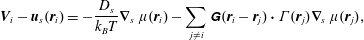 $$\begin{eqnarray}\boldsymbol{V}_{i}-\boldsymbol{u}_{s}(\boldsymbol{r}_{i})=-\frac{D_{s}}{k_{B}T}\unicode[STIX]{x1D735}_{s}\unicode[STIX]{x1D707}(\boldsymbol{r}_{i})-\mathop{\sum }_{j\neq i}\unicode[STIX]{x1D642}(\boldsymbol{r}_{i}-\boldsymbol{r}_{j})\boldsymbol{\cdot }\unicode[STIX]{x1D6E4}(\boldsymbol{r}_{j})\unicode[STIX]{x1D735}_{s}\unicode[STIX]{x1D707}(\boldsymbol{r}_{j}),\end{eqnarray}$$
where the final term reflects the surface velocity at $\boldsymbol{r}_{i}$
, established by all neighbouring surfactant molecules – with concentration
$\boldsymbol{r}_{i}$
, established by all neighbouring surfactant molecules – with concentration $\unicode[STIX]{x1D6E4}$
, each forced by
$\unicode[STIX]{x1D6E4}$
, each forced by $-\unicode[STIX]{x1D735}_{s}\unicode[STIX]{x1D707}$
. The Green’s function
$-\unicode[STIX]{x1D735}_{s}\unicode[STIX]{x1D707}$
. The Green’s function $\unicode[STIX]{x1D642}(\boldsymbol{r}_{i}-\boldsymbol{r}_{j})$
in this case gives the fluid velocity on the interface at
$\unicode[STIX]{x1D642}(\boldsymbol{r}_{i}-\boldsymbol{r}_{j})$
in this case gives the fluid velocity on the interface at $\boldsymbol{r}_{i}$
, driven by a force at
$\boldsymbol{r}_{i}$
, driven by a force at $\boldsymbol{r}_{j}$
on the fluid interface. The precise form of the Green’s function depends on the geometry of the interface, the subphase depth, etc. (§ 3.4.2) The added velocity due to hydrodynamic interactions, however, corresponds to a boundary integral solution (Pozrikidis Reference Pozrikidis1992) to the Stokes equations, where the fluid interface is driven by a specified traction:
$\boldsymbol{r}_{j}$
on the fluid interface. The precise form of the Green’s function depends on the geometry of the interface, the subphase depth, etc. (§ 3.4.2) The added velocity due to hydrodynamic interactions, however, corresponds to a boundary integral solution (Pozrikidis Reference Pozrikidis1992) to the Stokes equations, where the fluid interface is driven by a specified traction:
 $$\begin{eqnarray}\boldsymbol{f}_{M}\equiv \boldsymbol{n}\boldsymbol{\cdot }\unicode[STIX]{x1D748}|_{interface}=-\unicode[STIX]{x1D6E4}\unicode[STIX]{x1D735}_{s}\unicode[STIX]{x1D707},\end{eqnarray}$$
which, using the Gibbs adsorption relation (3.22), becomes
 $$\begin{eqnarray}\boldsymbol{f}_{M}=-\unicode[STIX]{x1D735}_{s}\unicode[STIX]{x1D6F1}=\unicode[STIX]{x1D735}_{s}\unicode[STIX]{x1D6FE}.\end{eqnarray}$$
The hydrodynamic coupling (3.76) between surfactant molecules is precisely equal to the net convective velocity driven by surface tension gradients. In other words, hydrodynamic coupling between surfactants is equivalent to the Marangoni flow driven on the interface by the surfactant monolayer.
Surface pressure gradients can drive or balance viscous shear stress following (3.78). Figure 10 illustrates two examples of the conjugate effects that usually go by the name of Marangoni, both of which involve surfactant gradients. Gradients in surface pressure may arise due to non-uniform surface concentrations $\unicode[STIX]{x1D6E4}(\boldsymbol{r}_{s})$
, or due to surface convective transport
$\unicode[STIX]{x1D6E4}(\boldsymbol{r}_{s})$
, or due to surface convective transport $\boldsymbol{u}_{s}\unicode[STIX]{x1D6E4}$
that establishes a concentration gradient. Depositing surfactant on an initially clean interface (figure 10
a) introduces a surface concentration gradient
$\boldsymbol{u}_{s}\unicode[STIX]{x1D6E4}$
that establishes a concentration gradient. Depositing surfactant on an initially clean interface (figure 10
a) introduces a surface concentration gradient $\unicode[STIX]{x1D735}_{s}\unicode[STIX]{x1D6E4}$
, and therefore a surface pressure gradient that exerts a traction
$\unicode[STIX]{x1D735}_{s}\unicode[STIX]{x1D6E4}$
, and therefore a surface pressure gradient that exerts a traction
 $$\begin{eqnarray}\boldsymbol{f}_{M}=\left.\unicode[STIX]{x1D702}\frac{\unicode[STIX]{x2202}\boldsymbol{v}}{\unicode[STIX]{x2202}z}\right|_{z=0}=-\unicode[STIX]{x1D735}_{s}\unicode[STIX]{x1D6F1}=-\frac{\unicode[STIX]{x2202}\unicode[STIX]{x1D6F1}}{\unicode[STIX]{x2202}\unicode[STIX]{x1D6E4}}\unicode[STIX]{x1D735}_{s}\unicode[STIX]{x1D6E4}.\end{eqnarray}$$
Flows are therefore driven down surface pressure (or surface concentration) gradients.
The functional form of $\unicode[STIX]{x1D6F1}(\unicode[STIX]{x1D6E4})$
depends on the particular surfactant isotherm (§ 2.4). It is common practice to assume an ideal gas monolayer, for which the Marangoni traction is
$\unicode[STIX]{x1D6F1}(\unicode[STIX]{x1D6E4})$
depends on the particular surfactant isotherm (§ 2.4). It is common practice to assume an ideal gas monolayer, for which the Marangoni traction is
 $$\begin{eqnarray}\boldsymbol{f}_{M}^{ideal}=-k_{B}T\unicode[STIX]{x1D735}_{s}\unicode[STIX]{x1D6E4}.\end{eqnarray}$$
As discussed in § 2.3, however, the ideal gas assumption rarely holds in practice, and more accurate models or measured values of $\unicode[STIX]{x2202}\unicode[STIX]{x1D6F1}/\unicode[STIX]{x2202}\unicode[STIX]{x1D6E4}$
would be more appropriate. For example, the Langmuir and Volmer isotherms give tractions
$\unicode[STIX]{x2202}\unicode[STIX]{x1D6F1}/\unicode[STIX]{x2202}\unicode[STIX]{x1D6E4}$
would be more appropriate. For example, the Langmuir and Volmer isotherms give tractions
 $$\begin{eqnarray}\boldsymbol{f}_{M}^{L}=-\frac{k_{B}T}{1-\unicode[STIX]{x1D6E4}/\unicode[STIX]{x1D6E4}_{\infty }}\unicode[STIX]{x1D735}_{s}\unicode[STIX]{x1D6E4}\quad \text{and}\quad \boldsymbol{f}_{M}^{V}=-\frac{k_{B}T}{(1-\unicode[STIX]{x1D6E4}/\unicode[STIX]{x1D6E4}_{\infty })^{2}}\unicode[STIX]{x1D735}_{s}\unicode[STIX]{x1D6E4},\end{eqnarray}$$
both of which recover the ideal gas limit when $\unicode[STIX]{x1D6E4}\ll \unicode[STIX]{x1D6E4}_{\infty }$
.
$\unicode[STIX]{x1D6E4}\ll \unicode[STIX]{x1D6E4}_{\infty }$
.
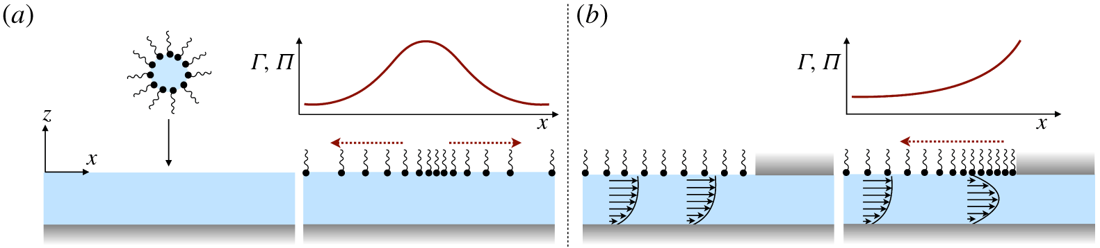
Figure 10. Two conjugate effects commonly termed ‘Marangoni’ effects: (a) A local increase in surfactant concentration, shown here by the addition of a surfactant-rich drop, establishes a surface concentration gradient (and, therefore, a surface pressure gradient) that drives an outward surface flow (red arrows). (b) Surface compression due to flow (in this case, towards an interfacial barrier) establishes a surface tension gradient due to non-uniform surface concentration. This introduces a reverse Marangoni flow that ‘immobilizes’ the surface.
The second example, shown in figure 10(b), resembles the so-called ‘Reynolds ridge’ (Scott Reference Scott1982) and involves flows that compress (or dilate) a surfactant-laden fluid interface against a floating barrier. Such a flow creates surface concentration gradients that act against the interfacial compression (or dilatation). Marangoni stresses therefore act like surface-excess elasticity (Langevin Reference Langevin2014), working to lessen surface compression or dilatation. In what follows, we quantify the degree to which reverse Marangoni flows resist inhomogeneous surface compression.
3.3.2 Marangoni numbers and surface incompressibility
Surfactant monolayers are far more compressible than 3-D fluids. Compressing an insoluble surfactant increases the surface concentration $\unicode[STIX]{x1D6E4}$
and thus the surface pressure
$\unicode[STIX]{x1D6E4}$
and thus the surface pressure $\unicode[STIX]{x1D6F1}$
. Additionally, many surfactants exhibit phase transitions (Kaganer, Möhwald & Dutta Reference Kaganer, Möhwald and Dutta1999) and surface-pressure-dependent surface viscosity (Kurtz, Lange & Fuller Reference Kurtz, Lange and Fuller2006; Kim et al.
Reference Kim, Choi, Zasadzinski and Squires2011) even under facile compression, as discussed in § 5. However, inhomogeneous compression of a surfactant monolayer drives reverse Marangoni flows that resist such deformations.
$\unicode[STIX]{x1D6F1}$
. Additionally, many surfactants exhibit phase transitions (Kaganer, Möhwald & Dutta Reference Kaganer, Möhwald and Dutta1999) and surface-pressure-dependent surface viscosity (Kurtz, Lange & Fuller Reference Kurtz, Lange and Fuller2006; Kim et al.
Reference Kim, Choi, Zasadzinski and Squires2011) even under facile compression, as discussed in § 5. However, inhomogeneous compression of a surfactant monolayer drives reverse Marangoni flows that resist such deformations.

Figure 11. Illustration of surfactant-induced incompressibility. (a) Motion of a probe establishes a surface concentration gradient, shown in top and side views. In a soluble monolayer with instantaneous adsorption/desorption, surface concentration gradients are rapidly eliminated. (b) In this limit, $\unicode[STIX]{x0394}\unicode[STIX]{x1D6F1}\approx 0$
and reverse Marangoni flows are absent. The surface flow has a non-zero divergence ahead and behind the disk. Bulk fluid flow is indicated by the dashed arrows and is indistinguishable from that corresponding to a stress-free clean interface. (c) By contrast, if the surfactant is insoluble, a surface concentration gradient is sustained, and (d) the surface pressure difference
$\unicode[STIX]{x0394}\unicode[STIX]{x1D6F1}\approx 0$
and reverse Marangoni flows are absent. The surface flow has a non-zero divergence ahead and behind the disk. Bulk fluid flow is indicated by the dashed arrows and is indistinguishable from that corresponding to a stress-free clean interface. (c) By contrast, if the surfactant is insoluble, a surface concentration gradient is sustained, and (d) the surface pressure difference $\unicode[STIX]{x0394}\unicode[STIX]{x1D6F1}$
generates a reverse Marangoni flow that resists interfacial compression/dilatation. The modified surface flow is divergence free, which changes the bulk flow by constraining it to flow in planes parallel to the interface (see discussion).
$\unicode[STIX]{x0394}\unicode[STIX]{x1D6F1}$
generates a reverse Marangoni flow that resists interfacial compression/dilatation. The modified surface flow is divergence free, which changes the bulk flow by constraining it to flow in planes parallel to the interface (see discussion).
For example, a disk of radius $R$
translating at velocity
$R$
translating at velocity $U$
within a planar surfactant-laden interface compresses the monolayer ahead of the disk, and dilates the monolayer in its rear (figure 11). The surfactant conservation equation for insoluble surfactants (3.10) at steady state, in the absence of surface diffusion, gives the surface divergence
$U$
within a planar surfactant-laden interface compresses the monolayer ahead of the disk, and dilates the monolayer in its rear (figure 11). The surfactant conservation equation for insoluble surfactants (3.10) at steady state, in the absence of surface diffusion, gives the surface divergence
 $$\begin{eqnarray}\unicode[STIX]{x1D735}_{s}\boldsymbol{\cdot }\boldsymbol{u}_{s}=-\frac{1}{\unicode[STIX]{x1D6E4}}\boldsymbol{u}_{s}\boldsymbol{\cdot }\unicode[STIX]{x1D735}_{s}\unicode[STIX]{x1D6E4}=-\frac{1}{E_{0}}\boldsymbol{u}_{s}\boldsymbol{\cdot }\unicode[STIX]{x1D735}_{s}\unicode[STIX]{x1D6F1},\end{eqnarray}$$
where $E_{0}$
is the Marangoni modulus (2.22). Balancing the surface pressure gradient
$E_{0}$
is the Marangoni modulus (2.22). Balancing the surface pressure gradient $\unicode[STIX]{x1D735}_{s}\unicode[STIX]{x1D6F1}$
in (3.82) with traction on the subphase via the Marangoni boundary condition (3.79) gives
$\unicode[STIX]{x1D735}_{s}\unicode[STIX]{x1D6F1}$
in (3.82) with traction on the subphase via the Marangoni boundary condition (3.79) gives
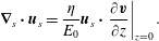 $$\begin{eqnarray}\unicode[STIX]{x1D735}_{s}\boldsymbol{\cdot }\boldsymbol{u}_{s}=\frac{\unicode[STIX]{x1D702}}{E_{0}}\boldsymbol{u}_{s}\boldsymbol{\cdot }\left.\frac{\unicode[STIX]{x2202}\boldsymbol{v}}{\unicode[STIX]{x2202}z}\right|_{z=0}.\end{eqnarray}$$
Non-dimensionalizing gives a dimensionless surface divergence
 $$\begin{eqnarray}\tilde{\unicode[STIX]{x1D735}}_{s}\boldsymbol{\cdot }\tilde{\boldsymbol{u}}_{s}=\frac{1}{Ma}\tilde{\boldsymbol{u}}_{s}\boldsymbol{\cdot }\left.\frac{\unicode[STIX]{x2202}\tilde{\boldsymbol{v}}}{\unicode[STIX]{x2202}\tilde{z}}\right|_{\tilde{z}=0},\end{eqnarray}$$
where the Marangoni number
 $$\begin{eqnarray}Ma=\frac{E_{0}}{\unicode[STIX]{x1D702}U}\end{eqnarray}$$
balances surface compressibility $E_{0}/R$
against viscous traction
$E_{0}/R$
against viscous traction $\unicode[STIX]{x1D702}U/R$
.
$\unicode[STIX]{x1D702}U/R$
.
In the large Marangoni number limit ( $Ma\gg 1$
), surfactant molecules resist compression so strongly that the surface flow is effectively divergence free. In other words, the surface is 2-D incompressible when the time scale to establish reverse Marangoni flows
$Ma\gg 1$
), surfactant molecules resist compression so strongly that the surface flow is effectively divergence free. In other words, the surface is 2-D incompressible when the time scale to establish reverse Marangoni flows
 $$\begin{eqnarray}\unicode[STIX]{x1D70F}_{m}=\frac{\unicode[STIX]{x1D702}R}{E_{0}}\end{eqnarray}$$
is much faster than the surface convection time scale $\unicode[STIX]{x1D70F}_{flow}=R/U$
, so that
$\unicode[STIX]{x1D70F}_{flow}=R/U$
, so that $Ma=\unicode[STIX]{x1D70F}_{flow}/\unicode[STIX]{x1D70F}_{m}\gg 1$
. Surface pressure then acts as a Lagrange multiplier to maintain surface incompressibility, much like bulk pressure in a 3-D fluid (figure 11). In unidirectional surface flows, such as in figure 10(b), surface incompressibility requires
$Ma=\unicode[STIX]{x1D70F}_{flow}/\unicode[STIX]{x1D70F}_{m}\gg 1$
. Surface pressure then acts as a Lagrange multiplier to maintain surface incompressibility, much like bulk pressure in a 3-D fluid (figure 11). In unidirectional surface flows, such as in figure 10(b), surface incompressibility requires $\boldsymbol{u}_{s}$
to be constant. Marangoni flows then ‘immobilize’ the interface, effectively modifying the interfacial boundary condition from a free surface (
$\boldsymbol{u}_{s}$
to be constant. Marangoni flows then ‘immobilize’ the interface, effectively modifying the interfacial boundary condition from a free surface ( $\unicode[STIX]{x2202}v/\unicode[STIX]{x2202}z=0$
) when
$\unicode[STIX]{x2202}v/\unicode[STIX]{x2202}z=0$
) when $Ma\ll 1$
to a rigid surface
$Ma\ll 1$
to a rigid surface $(u_{s}=v(0)=\text{const.})$
when
$(u_{s}=v(0)=\text{const.})$
when $Ma\gg 1$
.
$Ma\gg 1$
.
Insoluble surfactants are almost always surface incompressible around translating disks or particles. The Marangoni modulus of incredibly dilute monolayers with $\unicode[STIX]{x1D6E4}\sim 1/(100~\text{nm}^{2})$
in the ideal gas limit is
$\unicode[STIX]{x1D6E4}\sim 1/(100~\text{nm}^{2})$
in the ideal gas limit is $E_{0}^{ideal}=k_{B}T\unicode[STIX]{x1D6E4}\sim 0.04~\text{mN}~\text{m}^{-1}$
. Even for such dilute monolayers with immeasurably small surface pressures (
$E_{0}^{ideal}=k_{B}T\unicode[STIX]{x1D6E4}\sim 0.04~\text{mN}~\text{m}^{-1}$
. Even for such dilute monolayers with immeasurably small surface pressures ( $\unicode[STIX]{x1D6F1}\sim 40~\unicode[STIX]{x03BC}\text{N}~\text{m}^{-1}$
), a disk or particle must translate faster than
$\unicode[STIX]{x1D6F1}\sim 40~\unicode[STIX]{x03BC}\text{N}~\text{m}^{-1}$
), a disk or particle must translate faster than $4~\text{cm}~\text{s}^{-1}$
before
$4~\text{cm}~\text{s}^{-1}$
before $Ma\lesssim 1$
and the interface compresses. The Marangoni modulus of real surfactants is much larger than
$Ma\lesssim 1$
and the interface compresses. The Marangoni modulus of real surfactants is much larger than $E_{0}^{ideal}$
(table 1), with typical values of
$E_{0}^{ideal}$
(table 1), with typical values of $E_{0}\gtrsim 1~\text{mN}~\text{m}^{-1}$
(Arriaga et al.
Reference Arriaga, López-Montero, Ignés-Mullol and Monroy2010; Kotula & Anna Reference Kotula and Anna2016), so that insoluble monolayers are effectively surface incompressible unless
$E_{0}\gtrsim 1~\text{mN}~\text{m}^{-1}$
(Arriaga et al.
Reference Arriaga, López-Montero, Ignés-Mullol and Monroy2010; Kotula & Anna Reference Kotula and Anna2016), so that insoluble monolayers are effectively surface incompressible unless $U\gtrsim 1~\text{m}~\text{s}^{-1}$
.
$U\gtrsim 1~\text{m}~\text{s}^{-1}$
.
Even the slightest amount of insoluble surfactant, therefore, fundamentally changes the interfacial boundary condition on the bulk fluid flow. Stone & Masoud (Reference Stone and Masoud2015) illustrated the change in subphase flow by considering the continuity equation for the bulk fluid at the interface,
 $$\begin{eqnarray}\unicode[STIX]{x1D735}\boldsymbol{\cdot }\boldsymbol{v}|_{z=0}=\unicode[STIX]{x1D735}_{s}\boldsymbol{\cdot }\boldsymbol{v}|_{z=0}+\frac{\unicode[STIX]{x2202}w}{\unicode[STIX]{x2202}z}=0,\end{eqnarray}$$
where $w$
is the
$w$
is the $z$
-component of subphase fluid velocity
$z$
-component of subphase fluid velocity $\boldsymbol{v}$
. At the interface, the tangential velocity is
$\boldsymbol{v}$
. At the interface, the tangential velocity is $\boldsymbol{v}=\boldsymbol{u}_{s}$
, and thus surface incompressibility implies
$\boldsymbol{v}=\boldsymbol{u}_{s}$
, and thus surface incompressibility implies $\unicode[STIX]{x2202}w/\unicode[STIX]{x2202}z=0$
. The vertical velocity
$\unicode[STIX]{x2202}w/\unicode[STIX]{x2202}z=0$
. The vertical velocity $w$
vanishes at
$w$
vanishes at $z=0$
for an interface that does not deform out of plane, and along with
$z=0$
for an interface that does not deform out of plane, and along with $\unicode[STIX]{x2202}w/\unicode[STIX]{x2202}z=0$
requires that
$\unicode[STIX]{x2202}w/\unicode[STIX]{x2202}z=0$
requires that $w$
be zero throughout the subphase. Surface incompressibility therefore constrains subphase fluid to flow in planes parallel to the interface (figure 11
d). Such flows set up stronger velocity gradients, dissipating more energy than in surfactant-free systems, where flow in the bulk is three-dimensional (figure 11
b).
$w$
be zero throughout the subphase. Surface incompressibility therefore constrains subphase fluid to flow in planes parallel to the interface (figure 11
d). Such flows set up stronger velocity gradients, dissipating more energy than in surfactant-free systems, where flow in the bulk is three-dimensional (figure 11
b).
Insoluble surfactants therefore substantially modify subphase flow relative to surfactant-free systems, increasing the translational resistance of particles within monolayers. For example, the drag on a circular disk translating in an incompressible monolayer exceeds the drag in a clean interface by a factor of $3/2$
(§ 4.6). In some cases, this increase in translational resistance has been misattributed to surface rheology, going back to Plateau’s experiments with oscillating needles on interfaces (Scriven & Sternling Reference Scriven and Sternling1960), while in fact it arises due to Marangoni flows. Indeed, surface incompressibility increases the hydrodynamic drag on translating probes even for a completely inviscid surfactant, causing significant confusion in the measurement and interpretation of surface rheology of insoluble surfactants (Sickert & Rondelez (Reference Sickert and Rondelez2003), Fischer (Reference Fischer2004a
), and § 3.4).
$3/2$
(§ 4.6). In some cases, this increase in translational resistance has been misattributed to surface rheology, going back to Plateau’s experiments with oscillating needles on interfaces (Scriven & Sternling Reference Scriven and Sternling1960), while in fact it arises due to Marangoni flows. Indeed, surface incompressibility increases the hydrodynamic drag on translating probes even for a completely inviscid surfactant, causing significant confusion in the measurement and interpretation of surface rheology of insoluble surfactants (Sickert & Rondelez (Reference Sickert and Rondelez2003), Fischer (Reference Fischer2004a
), and § 3.4).
Soluble surfactants, on the other hand, may desorb (or adsorb) as the interface is compressed (or dilated) to restore equilibrium coverage (figure 11
a). The strength of the Marangoni stress then depends on the balance between surface advective and surfactant exchange fluxes. For small perturbations $\unicode[STIX]{x1D6FF}\unicode[STIX]{x1D6E4}$
in surface concentration around an equilibrium value
$\unicode[STIX]{x1D6FF}\unicode[STIX]{x1D6E4}$
in surface concentration around an equilibrium value $\unicode[STIX]{x1D6E4}_{0}$
, the surfactant balance (3.10) becomes
$\unicode[STIX]{x1D6E4}_{0}$
, the surfactant balance (3.10) becomes
 $$\begin{eqnarray}\unicode[STIX]{x1D6E4}_{0}\unicode[STIX]{x1D735}_{s}\boldsymbol{\cdot }\boldsymbol{u}_{s}=j_{n}=-\frac{\unicode[STIX]{x1D6FF}\unicode[STIX]{x1D6E4}}{\unicode[STIX]{x1D70F}_{s}},\end{eqnarray}$$
where $\unicode[STIX]{x1D70F}_{s}$
is the longer among kinetic and diffusive surfactant exchange times (3.56). Using (3.88) in the Marangoni boundary condition (3.79) gives
$\unicode[STIX]{x1D70F}_{s}$
is the longer among kinetic and diffusive surfactant exchange times (3.56). Using (3.88) in the Marangoni boundary condition (3.79) gives
 $$\begin{eqnarray}\left.\unicode[STIX]{x1D702}\frac{\unicode[STIX]{x2202}\boldsymbol{v}}{\unicode[STIX]{x2202}z}\right|_{z=0}=-\frac{\unicode[STIX]{x2202}\unicode[STIX]{x1D6F1}}{\unicode[STIX]{x2202}\unicode[STIX]{x1D6E4}}\unicode[STIX]{x1D735}_{s}(\unicode[STIX]{x1D6FF}\unicode[STIX]{x1D6E4})=E_{0}\unicode[STIX]{x1D70F}_{s}\unicode[STIX]{x1D735}_{s}(\unicode[STIX]{x1D735}_{s}\boldsymbol{\cdot }\boldsymbol{u}_{s}),\end{eqnarray}$$
where $E_{0}$
is the Marangoni modulus (2.22). Significantly, any finite adsorption time scale
$E_{0}$
is the Marangoni modulus (2.22). Significantly, any finite adsorption time scale $\unicode[STIX]{x1D70F}_{s}$
gives rise to a viscous-like force with apparent dilatational surface viscosity
$\unicode[STIX]{x1D70F}_{s}$
gives rise to a viscous-like force with apparent dilatational surface viscosity $E_{0}\unicode[STIX]{x1D70F}_{s}$
in (3.89) – a feature we will explore in detail in § 3.4.3. Non-dimensionalizing (3.89) gives
$E_{0}\unicode[STIX]{x1D70F}_{s}$
in (3.89) – a feature we will explore in detail in § 3.4.3. Non-dimensionalizing (3.89) gives
 $$\begin{eqnarray}\tilde{\unicode[STIX]{x1D735}}_{s}(\tilde{\unicode[STIX]{x1D735}}_{s}\boldsymbol{\cdot }\tilde{\boldsymbol{u}}_{s})=\frac{1}{Ma_{K}}\left.\frac{\unicode[STIX]{x2202}\tilde{\boldsymbol{v}}}{\unicode[STIX]{x2202}\tilde{z}}\right|_{\tilde{z}=0},\end{eqnarray}$$
where
 $$\begin{eqnarray}Ma_{K}=\frac{E_{0}\unicode[STIX]{x1D70F}_{s}}{\unicode[STIX]{x1D702}R}=\frac{\unicode[STIX]{x1D70F}_{s}}{\unicode[STIX]{x1D70F}_{m}}\end{eqnarray}$$
is a modified Marangoni number, that now compares the time scale $\unicode[STIX]{x1D70F}_{m}=\unicode[STIX]{x1D702}R/E_{0}$
to establish Marangoni flow with the time
$\unicode[STIX]{x1D70F}_{m}=\unicode[STIX]{x1D702}R/E_{0}$
to establish Marangoni flow with the time $\unicode[STIX]{x1D70F}_{s}$
for the surface to equilibrate via adsorption/desorption.
$\unicode[STIX]{x1D70F}_{s}$
for the surface to equilibrate via adsorption/desorption.
If a soluble monolayer equilibrates before Marangoni flows can be established ( $Ma_{K}\ll 1$
), then the surface behaves as if it is compressible. Equation (3.90) recovers the stress-free boundary condition as
$Ma_{K}\ll 1$
), then the surface behaves as if it is compressible. Equation (3.90) recovers the stress-free boundary condition as $Ma_{K}\rightarrow 0$
, and fluid flows behave approximately as though the interface were clean (figure 11
b). In this limit,
$Ma_{K}\rightarrow 0$
, and fluid flows behave approximately as though the interface were clean (figure 11
b). In this limit, $\unicode[STIX]{x1D6E4}$
and
$\unicode[STIX]{x1D6E4}$
and $\unicode[STIX]{x1D6F1}$
are largely unperturbed from the surfactant’s equilibrium isotherm. By contrast, if Marangoni flows are established before surfactants adsorb and desorb to equilibrate with the subphase concentration (
$\unicode[STIX]{x1D6F1}$
are largely unperturbed from the surfactant’s equilibrium isotherm. By contrast, if Marangoni flows are established before surfactants adsorb and desorb to equilibrate with the subphase concentration ( $Ma_{K}\gg 1$
), then the surface divergence is
$Ma_{K}\gg 1$
), then the surface divergence is
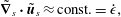 $$\begin{eqnarray}\tilde{\unicode[STIX]{x1D735}}_{s}\boldsymbol{\cdot }\tilde{\boldsymbol{u}}_{s}\approx \text{const.}=\dot{\unicode[STIX]{x1D716}},\end{eqnarray}$$
where $\dot{\unicode[STIX]{x1D716}}$
is a uniform compression or dilatation rate. In fact, interfaces with fixed area require
$\dot{\unicode[STIX]{x1D716}}$
is a uniform compression or dilatation rate. In fact, interfaces with fixed area require $\dot{\unicode[STIX]{x1D716}}=0$
, and the interface acts as incompressible.
$\dot{\unicode[STIX]{x1D716}}=0$
, and the interface acts as incompressible.
Finally, Marangoni flows may also be weakened by other surface processes, leading to alternative definitions of the Marangoni number. Table 3 summarizes common definitions of Marangoni numbers, obtained by comparing the Marangoni time scale $\unicode[STIX]{x1D70F}_{m}$
against competing system-specific surfactant processes. In each case, a large Marangoni number implies that the surfactant monolayer resists inhomogeneous surface compression or dilatation, and the interface can be approximated as 2-D incompressible. When Marangoni flows are weak, a fully compressible description becomes necessary (Barentin et al.
Reference Barentin, Ybert, Di Meglio and Joanny1999; Elfring, Leal & Squires Reference Elfring, Leal and Squires2016).
$\unicode[STIX]{x1D70F}_{m}$
against competing system-specific surfactant processes. In each case, a large Marangoni number implies that the surfactant monolayer resists inhomogeneous surface compression or dilatation, and the interface can be approximated as 2-D incompressible. When Marangoni flows are weak, a fully compressible description becomes necessary (Barentin et al.
Reference Barentin, Ybert, Di Meglio and Joanny1999; Elfring, Leal & Squires Reference Elfring, Leal and Squires2016).
Table 3. Common definitions of the Marangoni number, and their physical meaning. Temperature-dependent Marangoni effects are not considered here, and we list only the effects of composition dependence.

3.4 Surface rheology
Thus far, we have focused on surface processes such as adsorption/desorption, Marangoni flows and surface diffusion, which redistribute surfactants on the interface, and relax surface stresses in doing so. Additionally, however, some surfactants are known to exhibit surface rheology, exerting additional stresses when the surfactant layer deforms against itself.
The origin, existence and interpretation of surface rheology have been debated since the mid-19th century by the likes of Gibbs, Plateau, Marangoni and Rayleigh (Scriven & Sternling Reference Scriven and Sternling1960). Part of the controversy arises because even relatively simple flows excite multiple surfactant processes, or drive mixed surface deformations. For example, translating probes deform the surface via compression and dilatation in addition to shear, driving a combination of surface-viscous and Marangoni stresses. Surfactant-induced 2-D incompressibility fundamentally changes the subphase flow from the stress-free surface arising in the absence of surfactant, and changes the translational drag of probes substantially, even for completely inviscid surfactant monolayers (Fischer Reference Fischer2004a , and § 3.3.2). Experimental geometries specifically designed to drive purely shear deformations, like rotating disks (Choi et al. Reference Choi, Steltenkamp, Zasadzinski and Squires2011) or translating needles (Brooks et al. Reference Brooks, Fuller, Frank and Robertson1999), however, probe surface shear rheology unambiguously.
More subtle difficulties arise when surface viscosity is indirectly inferred from observable phenomena such as the settling velocity of surfactant-covered drops, or the drainage time of thin films. For example, recall from § 3.3.2 that Marangoni flows with finite-time adsorption introduces a surface-viscous-like force in the interfacial stress balance (3.89). In such systems, can this apparent surface dissipation alone account for all observed dynamics, or might the surfactant monolayer possess an ‘intrinsic’ surface dilatational viscosity? How does one differentiate between an ‘intrinsic’ and ‘apparent’ surface viscosity if both are present? In many cases, it might not be easy or even possible to deconvolve the origins of surface dissipation, leading to thousandfold discrepancies in surface viscosities interpreted from decades of experiments (Stevenson Reference Stevenson2005).
In this section, we will explore the simplest of surface rheological models – monolayers that behave like 2-D Newtonian fluids. We use this model to (a) interpret experiments that confirm and characterize ‘intrinsic’ surface shear viscosities, (b) illustrate the relative contributions of subphase and interfacial viscous resistance to flow and (c) highlight difficulties in determining ‘intrinsic’ surface dilatational viscosities from experiments. The 2-D Newtonian model will also set the stage for treating surface rheology in the paradigmatic problems outlined in § 4. The richer and more complex surface rheological responses that arise more commonly are described in § 5.
3.4.1 The Boussinesq–Scriven model
Boussinesq (Reference Boussinesq1913) was the first to explicitly account for a viscous-like resistance to surface dilatation, using it to explain the anomalous settling velocity of drops (§ 4.1). Scriven (Reference Scriven1960) generalized Boussinesq’s model by treating the interfacial layer as a 2-D Newtonian fluid with intrinsic surface shear ( $\unicode[STIX]{x1D702}_{s}$
) and surface dilatational (
$\unicode[STIX]{x1D702}_{s}$
) and surface dilatational ( $\unicode[STIX]{x1D705}_{s}$
) viscosities, both with dimensions of 3-D viscosity
$\unicode[STIX]{x1D705}_{s}$
) viscosities, both with dimensions of 3-D viscosity $\times$
length, so that the extra rheological stress
$\times$
length, so that the extra rheological stress $\unicode[STIX]{x1D749}_{rheo}$
in (3.8) is Newtonian
$\unicode[STIX]{x1D749}_{rheo}$
in (3.8) is Newtonian
 $$\begin{eqnarray}\unicode[STIX]{x1D749}_{rheo}=[(\unicode[STIX]{x1D705}_{s}-\unicode[STIX]{x1D702}_{s})\unicode[STIX]{x1D735}_{s}\boldsymbol{\cdot }\boldsymbol{u})]\unicode[STIX]{x1D644}_{s}+\unicode[STIX]{x1D702}_{s}[\unicode[STIX]{x1D735}_{s}\boldsymbol{u}\boldsymbol{\cdot }\unicode[STIX]{x1D644}_{s}+\unicode[STIX]{x1D644}_{s}\boldsymbol{\cdot }(\unicode[STIX]{x1D735}_{s}\boldsymbol{u})^{\text{T}}],\end{eqnarray}$$
where $\unicode[STIX]{x1D644}_{s}=\unicode[STIX]{x1D644}-\boldsymbol{n}\boldsymbol{n}$
is the surface identity tensor. Using (3.93) in the surface stress balance (3.8) for a planar liquid–air interface gives
$\unicode[STIX]{x1D644}_{s}=\unicode[STIX]{x1D644}-\boldsymbol{n}\boldsymbol{n}$
is the surface identity tensor. Using (3.93) in the surface stress balance (3.8) for a planar liquid–air interface gives
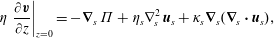 $$\begin{eqnarray}\unicode[STIX]{x1D702}\left.\frac{\unicode[STIX]{x2202}\boldsymbol{v}}{\unicode[STIX]{x2202}z}\right|_{z=0}=-\unicode[STIX]{x1D735}_{s}\unicode[STIX]{x1D6F1}+\unicode[STIX]{x1D702}_{s}\unicode[STIX]{x1D6FB}_{s}^{2}\boldsymbol{u}_{s}+\unicode[STIX]{x1D705}_{s}\unicode[STIX]{x1D735}_{s}(\unicode[STIX]{x1D735}_{s}\boldsymbol{\cdot }\boldsymbol{u}_{s}),\end{eqnarray}$$
which is the 2-D analogue of the Stokes equation for compressible fluids, with viscous traction from the subphase entering as a body force. More generally, out-of-plane deformations and 2-D viscous flow along curved interfaces introduce additional forces that have no analogue in 3-D Newtonian fluids (Scriven Reference Scriven1960; Aris Reference Aris1962; Edwards, Brenner & Wasan Reference Edwards, Brenner and Wasan1991; Slattery et al. Reference Slattery, Sagis and Oh2007).
The Boussinesq–Scriven model simplifies in many typical surfactant systems. As discussed in § 3.3.2, insoluble surfactants almost always behave as surface incompressible, in which case (3.94) reduces to the incompressible 2-D Stokes equation, forced by viscous traction from the subphase
 $$\begin{eqnarray}\unicode[STIX]{x1D735}_{s}\unicode[STIX]{x1D6F1}=\unicode[STIX]{x1D702}_{s}\unicode[STIX]{x1D6FB}_{s}^{2}\boldsymbol{u}_{s}-\unicode[STIX]{x1D702}\left.\frac{\unicode[STIX]{x2202}\boldsymbol{v}}{\unicode[STIX]{x2202}z}\right|_{z=0},\quad \unicode[STIX]{x1D735}_{s}\boldsymbol{\cdot }\boldsymbol{u}_{s}=0.\end{eqnarray}$$
Surface pressure then acts to enforce 2-D incompressibility, analogous to bulk pressure in a 3-D incompressible fluid.
Solving such problems is generally difficult, because two- and three-dimensional Stokes flows must be solved separately, but coupled via boundary conditions enforcing surface incompressibility and subphase traction. In systems where the subphase is very shallow, however, this coupling simplifies significantly, because the lubrication approximation relates the subphase velocity gradient to interfacial velocity and the subphase depth $H$
,
$H$
,
 $$\begin{eqnarray}\left.\frac{\unicode[STIX]{x2202}\boldsymbol{v}}{\unicode[STIX]{x2202}z}\right|_{z=0}=\frac{\boldsymbol{u}_{s}}{H},\end{eqnarray}$$
in which case the subphase flow need not be solved explicitly (Evans & Sackmann Reference Evans and Sackmann1988). The lubrication approximation is particularly useful for compressible monolayers, where eliminating $\boldsymbol{u}$
permits analytical solutions (Barentin et al.
Reference Barentin, Ybert, Di Meglio and Joanny1999; Elfring et al.
Reference Elfring, Leal and Squires2016).
$\boldsymbol{u}$
permits analytical solutions (Barentin et al.
Reference Barentin, Ybert, Di Meglio and Joanny1999; Elfring et al.
Reference Elfring, Leal and Squires2016).
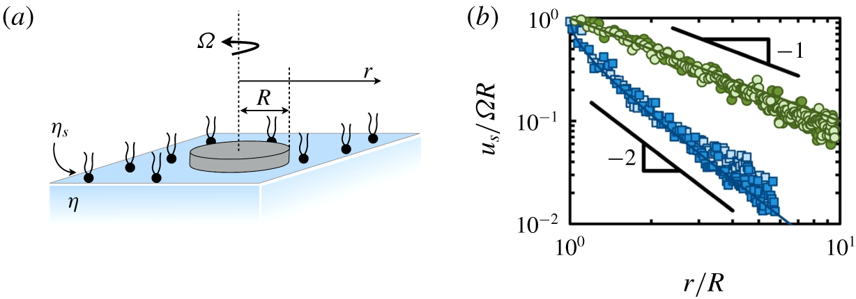
Figure 12. (a) A disk of radius $R$
rotating at a constant angular velocity
$R$
rotating at a constant angular velocity $\unicode[STIX]{x1D6FA}$
within a monolayer of surface shear viscosity
$\unicode[STIX]{x1D6FA}$
within a monolayer of surface shear viscosity $\unicode[STIX]{x1D702}_{s}$
. (b) Surface velocity
$\unicode[STIX]{x1D702}_{s}$
. (b) Surface velocity $u_{s}$
follows (3.100) when subphase dominant (
$u_{s}$
follows (3.100) when subphase dominant ( $Bq\ll 1$
, blue squares) and (3.101) when interface dominant (
$Bq\ll 1$
, blue squares) and (3.101) when interface dominant ( $Bq\gg 1$
, green circles); adapted from Zell et al. (Reference Zell, Nowbahar, Mansard, Leal, Deshmukh, Mecca, Tucker and Squires2014).
$Bq\gg 1$
, green circles); adapted from Zell et al. (Reference Zell, Nowbahar, Mansard, Leal, Deshmukh, Mecca, Tucker and Squires2014).
3.4.2 Two-dimensional versus three-dimensional hydrodynamics and the Boussinesq number
Momentum propagation through a viscous interfacial layer fundamentally modifies familiar 3-D fluid dynamics, even when no other surfactant process is excited. For example, pure shear deformations like the swirling flow driven by rotating a circular disk at an interface (figure 12) do not generate surface concentration gradients, and thus do not give rise to Marangoni stresses. The planar Boussinesq–Scriven equation (3.94) then becomes
 $$\begin{eqnarray}\left.\unicode[STIX]{x1D702}\frac{\unicode[STIX]{x2202}\boldsymbol{v}}{\unicode[STIX]{x2202}z}\right|_{z=0}=\unicode[STIX]{x1D702}_{s}\unicode[STIX]{x1D6FB}_{s}^{2}\boldsymbol{u}_{s},\end{eqnarray}$$
which couples to the Stokes equations for $\boldsymbol{u}$
in the subphase. Flow is driven by the rotation of a disk of radius
$\boldsymbol{u}$
in the subphase. Flow is driven by the rotation of a disk of radius $R$
at constant angular velocity
$R$
at constant angular velocity $\unicode[STIX]{x1D6FA}$
:
$\unicode[STIX]{x1D6FA}$
: $\boldsymbol{u}_{s}(r\leqslant R)=\unicode[STIX]{x1D6FA}r\hat{\unicode[STIX]{x1D73D}}$
. Non-dimensionalizing (3.97) gives
$\boldsymbol{u}_{s}(r\leqslant R)=\unicode[STIX]{x1D6FA}r\hat{\unicode[STIX]{x1D73D}}$
. Non-dimensionalizing (3.97) gives
 $$\begin{eqnarray}\left.\frac{\unicode[STIX]{x2202}\tilde{\boldsymbol{v}}}{\unicode[STIX]{x2202}\tilde{z}}\right|_{\tilde{z}=0}=Bq\tilde{\unicode[STIX]{x1D6FB}}_{s}^{2}\tilde{\boldsymbol{u}}_{s},\end{eqnarray}$$
where the Boussinesq number,
 $$\begin{eqnarray}Bq=\frac{\unicode[STIX]{x1D702}_{s}}{\unicode[STIX]{x1D702}R},\end{eqnarray}$$
compares surface and subphase viscous stresses.
Subphase-dominant flows ( $Bq\ll 1$
) in pure shear recover the stress-free condition at the interface. Solving the Stokes equations in the subphase with a stress-free interface driven by a rotating disk gives (Goodrich Reference Goodrich1969)
$Bq\ll 1$
) in pure shear recover the stress-free condition at the interface. Solving the Stokes equations in the subphase with a stress-free interface driven by a rotating disk gives (Goodrich Reference Goodrich1969)
 $$\begin{eqnarray}\boldsymbol{u}_{s}(Bq=0)=\frac{2\unicode[STIX]{x1D6FA}R}{\unicode[STIX]{x03C0}}\left[\frac{r}{R}\sin ^{-1}\left(\frac{R}{r}\right)-\left(1-\frac{R^{2}}{r^{2}}\right)^{1/2}\right]\hat{\unicode[STIX]{x1D73D}}\xrightarrow[{}]{r\gg R}\frac{4\unicode[STIX]{x1D6FA}}{3\unicode[STIX]{x03C0}}\frac{R^{3}}{r^{2}}\hat{\unicode[STIX]{x1D73D}}.\end{eqnarray}$$
The velocity field due to rotation decays as $1/r^{2}$
in the absence of surface excess rheological stresses, as expected in Stokes flow (Guazzelli & Morris Reference Guazzelli and Morris2012).
$1/r^{2}$
in the absence of surface excess rheological stresses, as expected in Stokes flow (Guazzelli & Morris Reference Guazzelli and Morris2012).
By contrast, (3.98) implies that $\unicode[STIX]{x1D6FB}_{s}^{2}\boldsymbol{u}_{s}\approx \mathbf{0}$
when the flow is interface dominant (
$\unicode[STIX]{x1D6FB}_{s}^{2}\boldsymbol{u}_{s}\approx \mathbf{0}$
when the flow is interface dominant ( $Bq\gg 1$
), and
$Bq\gg 1$
), and
 $$\begin{eqnarray}\boldsymbol{u}_{s}(Bq\rightarrow \infty )=\frac{\unicode[STIX]{x1D6FA}R^{2}}{r}\hat{\unicode[STIX]{x1D73D}}.\end{eqnarray}$$
A viscous interfacial layer propagates momentum more extensively within the interface, resulting in a slower decay ( ${\sim}1/r$
) of the surface velocity field relative to (3.100), as shown in figure 12(b). The torque required to sustain constant rotation transitions from
${\sim}1/r$
) of the surface velocity field relative to (3.100), as shown in figure 12(b). The torque required to sustain constant rotation transitions from ${\sim}R^{3}$
for an inviscid interface (
${\sim}R^{3}$
for an inviscid interface ( $Bq=0$
) to
$Bq=0$
) to ${\sim}R^{2}$
for a viscous monolayer (
${\sim}R^{2}$
for a viscous monolayer ( $Bq\rightarrow \infty$
; see § 4.6). This striking difference arises in systems where no other surfactant transport process – e.g. Marangoni flow, adsorption/desorption, surface dilatation – is active. Measurements of the rotational torque and flow field around a rotating disk can thus unambiguously and quantitatively detect surface shear viscosity (Choi et al.
Reference Choi, Steltenkamp, Zasadzinski and Squires2011; Zell et al.
Reference Zell, Nowbahar, Mansard, Leal, Deshmukh, Mecca, Tucker and Squires2014).
$Bq\rightarrow \infty$
; see § 4.6). This striking difference arises in systems where no other surfactant transport process – e.g. Marangoni flow, adsorption/desorption, surface dilatation – is active. Measurements of the rotational torque and flow field around a rotating disk can thus unambiguously and quantitatively detect surface shear viscosity (Choi et al.
Reference Choi, Steltenkamp, Zasadzinski and Squires2011; Zell et al.
Reference Zell, Nowbahar, Mansard, Leal, Deshmukh, Mecca, Tucker and Squires2014).
The translation of a particle embedded within a monolayer is more complex, as it deforms the surface via compression, dilation and extension, in addition to shear. Even in the seemingly simpler case of insoluble (and, therefore, 2-D incompressible from § 3.3.2) monolayers, translation introduces subtleties due to momentum transfer between a surface-shear-viscous interface and the underlying 3-D fluid.
Saffman & Delbrück (Reference Saffman and Delbrück1975) noticed this transition from 2-D to 3-D hydrodynamics in their seminal work on particle diffusion in biological membranes. The incompressible Boussinesq–Scriven equation (3.95) decouples from the subphase in the interface-dominant ( $Bq\rightarrow \infty$
) limit. However, there is no solution for steady translation of a cylinder in 2-D creeping flow (Leal Reference Leal2007, the ‘Stokes paradox’). Saffman (Reference Saffman1976) recognized that subphase viscous stresses (
$Bq\rightarrow \infty$
) limit. However, there is no solution for steady translation of a cylinder in 2-D creeping flow (Leal Reference Leal2007, the ‘Stokes paradox’). Saffman (Reference Saffman1976) recognized that subphase viscous stresses ( ${\sim}\unicode[STIX]{x1D702}U\ell _{SD}$
) eventually catch up with surface-viscous stresses (
${\sim}\unicode[STIX]{x1D702}U\ell _{SD}$
) eventually catch up with surface-viscous stresses ( ${\sim}\unicode[STIX]{x1D702}_{s}U$
) beyond a distance
${\sim}\unicode[STIX]{x1D702}_{s}U$
) beyond a distance
 $$\begin{eqnarray}\ell _{SD}=\frac{\unicode[STIX]{x1D702}_{s}}{\unicode[STIX]{x1D702}},\end{eqnarray}$$
ultimately regularizing the divergence inherent to 2-D Stokes flow. Surface viscous stresses dominate within the Saffman–Delbrück length $\ell _{SD}$
, and viscous traction from the subphase prevail beyond
$\ell _{SD}$
, and viscous traction from the subphase prevail beyond $\ell _{SD}$
.
$\ell _{SD}$
.
The cross-over from 2-D to 3-D hydrodynamics is evident in the flow driven by a tangential point force on the interface (Lubensky & Goldstein Reference Lubensky and Goldstein1996; Levine & MacKintosh Reference Levine and MacKintosh2002; Fischer Reference Fischer2004b ; Oppenheimer & Diamant Reference Oppenheimer and Diamant2009). Velocity fields driven by arbitrarily shaped particles moving on an interface can be constructed using appropriate boundary integrals of the point-force solution (§ 4.6).
An incompressible Newtonian monolayer along the $x$
–
$x$
– $y$
plane acted upon by an in-plane point force
$y$
plane acted upon by an in-plane point force $\boldsymbol{F}$
at
$\boldsymbol{F}$
at $\boldsymbol{x}_{0}$
is governed by
$\boldsymbol{x}_{0}$
is governed by
 $$\begin{eqnarray}\unicode[STIX]{x1D735}_{s}\unicode[STIX]{x1D6F1}=\unicode[STIX]{x1D702}_{s}\unicode[STIX]{x1D6FB}_{s}^{2}\boldsymbol{u}_{s}-\unicode[STIX]{x1D702}\left.\frac{\unicode[STIX]{x2202}\boldsymbol{v}}{\unicode[STIX]{x2202}z}\right|_{z=0}+\boldsymbol{F}\unicode[STIX]{x1D6FF}(\boldsymbol{r}),\quad \unicode[STIX]{x1D735}_{s}\boldsymbol{\cdot }\boldsymbol{u}_{s}=0,\end{eqnarray}$$
where $\boldsymbol{r}=\boldsymbol{x}-\boldsymbol{x}_{0}$
. The two-dimensional Fourier transform,
$\boldsymbol{r}=\boldsymbol{x}-\boldsymbol{x}_{0}$
. The two-dimensional Fourier transform,
 $$\begin{eqnarray}\unicode[STIX]{x1D719}(\boldsymbol{x})=\int \hat{\unicode[STIX]{x1D719}}(\boldsymbol{k})\text{e}^{\text{i}\boldsymbol{k}\boldsymbol{\cdot }\boldsymbol{r}}\,\text{d}\boldsymbol{k},\end{eqnarray}$$
is defined so that $\boldsymbol{k}\boldsymbol{\cdot }\hat{\boldsymbol{e}}_{z}=0$
, and transforms (3.103) to give
$\boldsymbol{k}\boldsymbol{\cdot }\hat{\boldsymbol{e}}_{z}=0$
, and transforms (3.103) to give
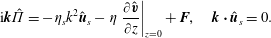 $$\begin{eqnarray}\text{i}\boldsymbol{k}\hat{\unicode[STIX]{x1D6F1}}=-\unicode[STIX]{x1D702}_{s}k^{2}\hat{\boldsymbol{u}}_{s}-\unicode[STIX]{x1D702}\left.\frac{\unicode[STIX]{x2202}\hat{\boldsymbol{v}}}{\unicode[STIX]{x2202}z}\right|_{z=0}+\boldsymbol{F},\quad \boldsymbol{k}\boldsymbol{\cdot }\hat{\boldsymbol{u}}_{s}=0.\end{eqnarray}$$
The (3-D) hydrodynamic pressure field $p$
associated with flow on an incompressible surface is a constant everywhere (Stone & Ajdari Reference Stone and Ajdari1998), such that momentum balance for Stokes flow in the bulk reduces to Laplace’s equation:
$p$
associated with flow on an incompressible surface is a constant everywhere (Stone & Ajdari Reference Stone and Ajdari1998), such that momentum balance for Stokes flow in the bulk reduces to Laplace’s equation: $\unicode[STIX]{x1D6FB}^{2}\boldsymbol{v}=\mathbf{0}$
. If the subphase extends to a finite depth
$\unicode[STIX]{x1D6FB}^{2}\boldsymbol{v}=\mathbf{0}$
. If the subphase extends to a finite depth $H$
such that
$H$
such that $\boldsymbol{v}(-H)=\mathbf{0}$
, then
$\boldsymbol{v}(-H)=\mathbf{0}$
, then
 $$\begin{eqnarray}\hat{\boldsymbol{v}}(\boldsymbol{k})=\left(\frac{\sinh (kz)}{\tanh (kH)}+\cosh (kz)\right)\hat{\boldsymbol{u}}_{s}(\boldsymbol{k}).\end{eqnarray}$$
Using (3.106) in (3.105) and eliminating $\hat{\unicode[STIX]{x1D6F1}}$
by premultiplying by
$\hat{\unicode[STIX]{x1D6F1}}$
by premultiplying by $\unicode[STIX]{x1D644}-\boldsymbol{k}\boldsymbol{k}/k^{2}$
gives
$\unicode[STIX]{x1D644}-\boldsymbol{k}\boldsymbol{k}/k^{2}$
gives
 $$\begin{eqnarray}\hat{\boldsymbol{u}}_{s}(\boldsymbol{k})=\hat{\unicode[STIX]{x1D642}}(\boldsymbol{k})\boldsymbol{\cdot }\boldsymbol{F}=\left[\frac{k^{2}\unicode[STIX]{x1D644}-\boldsymbol{k}\boldsymbol{k}}{k^{4}\unicode[STIX]{x1D702}_{s}+k^{3}\unicode[STIX]{x1D702}\coth (kH)}\right]\boldsymbol{\cdot }\boldsymbol{F}.\end{eqnarray}$$
The Green’s function $\hat{\unicode[STIX]{x1D642}}(\boldsymbol{k})$
depends on the ratio
$\hat{\unicode[STIX]{x1D642}}(\boldsymbol{k})$
depends on the ratio $k\unicode[STIX]{x1D702}_{s}/\unicode[STIX]{x1D702}$
, which is the Boussinesq number (3.99) for a length scale
$k\unicode[STIX]{x1D702}_{s}/\unicode[STIX]{x1D702}$
, which is the Boussinesq number (3.99) for a length scale $\unicode[STIX]{x1D706}=2\unicode[STIX]{x03C0}/k$
. In real space, the second-order tensor
$\unicode[STIX]{x1D706}=2\unicode[STIX]{x03C0}/k$
. In real space, the second-order tensor $\unicode[STIX]{x1D642}(\boldsymbol{r})$
is the surface analogue of the Oseen tensor in classical hydrodynamics. However, inverting
$\unicode[STIX]{x1D642}(\boldsymbol{r})$
is the surface analogue of the Oseen tensor in classical hydrodynamics. However, inverting $\hat{\unicode[STIX]{x1D642}}$
is not straightforward except in specific limits. We will focus on the deep subphase limit (
$\hat{\unicode[STIX]{x1D642}}$
is not straightforward except in specific limits. We will focus on the deep subphase limit ( $H\rightarrow \infty$
), where the inverse transform gives (Lubensky & Goldstein Reference Lubensky and Goldstein1996; Fischer Reference Fischer2004b
; Levine & MacKintosh Reference Levine and MacKintosh2002)
$H\rightarrow \infty$
), where the inverse transform gives (Lubensky & Goldstein Reference Lubensky and Goldstein1996; Fischer Reference Fischer2004b
; Levine & MacKintosh Reference Levine and MacKintosh2002)
 $$\begin{eqnarray}\boldsymbol{u}_{s}(\boldsymbol{x})=\frac{1}{4\unicode[STIX]{x1D702}_{s}}\left[\unicode[STIX]{x1D707}_{\Vert }(r)\frac{\boldsymbol{r}\boldsymbol{r}}{r^{2}}+\unicode[STIX]{x1D707}_{\bot }(r)\left(\unicode[STIX]{x1D644}-\frac{\boldsymbol{r}\boldsymbol{r}}{r^{2}}\right)\right]\boldsymbol{\cdot }\boldsymbol{F},\end{eqnarray}$$
where $r=|\boldsymbol{r}|$
. The mobility coefficients
$r=|\boldsymbol{r}|$
. The mobility coefficients $\unicode[STIX]{x1D707}_{\Vert }$
and
$\unicode[STIX]{x1D707}_{\Vert }$
and $\unicode[STIX]{x1D707}_{\bot }$
are
$\unicode[STIX]{x1D707}_{\bot }$
are
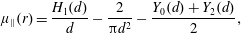 $$\begin{eqnarray}\displaystyle & \displaystyle \unicode[STIX]{x1D707}_{\Vert }(r)=\frac{H_{1}(d)}{d}-\frac{2}{\unicode[STIX]{x03C0}d^{2}}-\frac{Y_{0}(d)+Y_{2}(d)}{2}, & \displaystyle\end{eqnarray}$$
 $$\begin{eqnarray}\displaystyle & \displaystyle \unicode[STIX]{x1D707}_{\bot }(r)=H_{0}(d)-\frac{H_{1}(d)}{d}+\frac{2}{\unicode[STIX]{x03C0}d^{2}}-\frac{Y_{0}(d)-Y_{2}(d)}{2}, & \displaystyle\end{eqnarray}$$ $H_{\unicode[STIX]{x1D708}}$
and
$H_{\unicode[STIX]{x1D708}}$
and $Y_{\unicode[STIX]{x1D708}}$
are, respectively, Struve functions and Bessel functions of the second kind of order
$Y_{\unicode[STIX]{x1D708}}$
are, respectively, Struve functions and Bessel functions of the second kind of order $\unicode[STIX]{x1D708}$
, and
$\unicode[STIX]{x1D708}$
, and  $$\begin{eqnarray}d=\frac{r\unicode[STIX]{x1D702}}{\unicode[STIX]{x1D702}_{s}}=\frac{r}{\ell _{SD}},\end{eqnarray}$$
is distance scaled by the Saffman–Delbrück length $\ell _{SD}$
(3.102). Alternatively, non-dimensionalizing
$\ell _{SD}$
(3.102). Alternatively, non-dimensionalizing $r$
by the probe size
$r$
by the probe size $R$
makes
$R$
makes $d$
in (3.110) equivalent to
$d$
in (3.110) equivalent to
 $$\begin{eqnarray}d=\frac{\tilde{r}}{Bq},\end{eqnarray}$$
where $Bq=\unicode[STIX]{x1D702}_{s}/\unicode[STIX]{x1D702}R$
is the Boussinesq number (3.99).
$Bq=\unicode[STIX]{x1D702}_{s}/\unicode[STIX]{x1D702}R$
is the Boussinesq number (3.99).
Momentum transport is interface-dominated over length scales smaller than $\ell _{SD}$
(
$\ell _{SD}$
( $d\ll 1$
or
$d\ll 1$
or $Bq\gg 1$
), and the mobility coefficients (3.109) become
$Bq\gg 1$
), and the mobility coefficients (3.109) become
 $$\begin{eqnarray}\displaystyle & \displaystyle \unicode[STIX]{x1D707}_{\Vert }(r\ll \ell _{SD})\approx \frac{1}{\unicode[STIX]{x03C0}}\left(-\text{log}\left(\frac{d}{2}\right)+\frac{1}{2}-\unicode[STIX]{x1D6FE}_{E}\right), & \displaystyle\end{eqnarray}$$
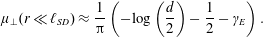 $$\begin{eqnarray}\displaystyle & \displaystyle \unicode[STIX]{x1D707}_{\bot }(r\ll \ell _{SD})\approx \frac{1}{\unicode[STIX]{x03C0}}\left(-\text{log}\left(\frac{d}{2}\right)-\frac{1}{2}-\unicode[STIX]{x1D6FE}_{E}\right). & \displaystyle\end{eqnarray}$$ $Bq\rightarrow \infty$
(or
$Bq\rightarrow \infty$
(or $d\rightarrow 0$
) limit is then
$d\rightarrow 0$
) limit is then  $$\begin{eqnarray}\boldsymbol{u}_{s}(\boldsymbol{x},Bq\rightarrow \infty )=\frac{1}{4\unicode[STIX]{x03C0}\unicode[STIX]{x1D702}_{s}}\left[-\text{log}(r)\unicode[STIX]{x1D644}+\frac{\boldsymbol{r}\boldsymbol{r}}{r^{2}}\right]\boldsymbol{\cdot }\boldsymbol{F},\end{eqnarray}$$
which is, indeed, the 2-D Stokeslet.
The logarithmic divergence in (3.113) as $r\rightarrow \infty$
reflects the Stokes paradox, which is here resolved by viscous traction from the subphase. Subphase viscous stresses become dominant over length scales larger than
$r\rightarrow \infty$
reflects the Stokes paradox, which is here resolved by viscous traction from the subphase. Subphase viscous stresses become dominant over length scales larger than $\ell _{SD}$
(
$\ell _{SD}$
( $d\gg 1$
or
$d\gg 1$
or $Bq\ll 1$
), in which case
$Bq\ll 1$
), in which case
 $$\begin{eqnarray}\displaystyle & \displaystyle \unicode[STIX]{x1D707}_{\Vert }(r\gg \ell _{SD})\approx \frac{2}{\unicode[STIX]{x03C0}d}-\frac{2}{\unicode[STIX]{x03C0}d^{2}}, & \displaystyle\end{eqnarray}$$
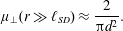 $$\begin{eqnarray}\displaystyle & \displaystyle \unicode[STIX]{x1D707}_{\bot }(r\gg \ell _{SD})\approx \frac{2}{\unicode[STIX]{x03C0}d^{2}}. & \displaystyle\end{eqnarray}$$
 $$\begin{eqnarray}\boldsymbol{u}_{s}(\boldsymbol{x},Bq\rightarrow 0)=\frac{1}{2\unicode[STIX]{x03C0}\unicode[STIX]{x1D702}}\frac{\boldsymbol{r}\boldsymbol{r}}{r^{3}}\boldsymbol{\cdot }\boldsymbol{F}\end{eqnarray}$$
in the surface-inviscid limit ( $Bq\rightarrow 0$
). Notably, (3.115) is not a 2-D slice of the flow due to a 3-D Stokeslet – surface incompressibility (§ 3.3.2) modifies fluid streamlines to ensure that the resultant velocity profile is surface-divergence free (figure 11).
$Bq\rightarrow 0$
). Notably, (3.115) is not a 2-D slice of the flow due to a 3-D Stokeslet – surface incompressibility (§ 3.3.2) modifies fluid streamlines to ensure that the resultant velocity profile is surface-divergence free (figure 11).
Prasad, Koehler & Weeks (Reference Prasad, Koehler and Weeks2006) experimentally mapped out surface velocities on surface-viscous protein monolayers via passive (colloid-tracking) two-particle microrheology. The displacement correlations between two points on the interface along and perpendicular to the line joining their centres are proportional to mobility coefficients $\unicode[STIX]{x1D707}_{\Vert }$
and
$\unicode[STIX]{x1D707}_{\Vert }$
and $\unicode[STIX]{x1D707}_{\bot }$
, respectively. Experiments over a wide range of surface viscosities (from
$\unicode[STIX]{x1D707}_{\bot }$
, respectively. Experiments over a wide range of surface viscosities (from $O(1)\,\text{nN}~\text{s}~\text{m}^{-1}$
to
$O(1)\,\text{nN}~\text{s}~\text{m}^{-1}$
to $O(1)~\unicode[STIX]{x03BC}\text{N}~\text{s}~\text{m}^{-1}$
) clearly show this transition from a logarithmic decay in the interface-dominated regime to
$O(1)~\unicode[STIX]{x03BC}\text{N}~\text{s}~\text{m}^{-1}$
) clearly show this transition from a logarithmic decay in the interface-dominated regime to $\unicode[STIX]{x1D707}_{\Vert }\sim 1/r$
and
$\unicode[STIX]{x1D707}_{\Vert }\sim 1/r$
and $\unicode[STIX]{x1D707}_{\bot }\sim 1/r^{2}$
when subphase stresses dominate (figure 13). Surface streamlines following (3.108) also transition distinctly between subphase-dominant and interface-dominant flows (figure 14).
$\unicode[STIX]{x1D707}_{\bot }\sim 1/r^{2}$
when subphase stresses dominate (figure 13). Surface streamlines following (3.108) also transition distinctly between subphase-dominant and interface-dominant flows (figure 14).
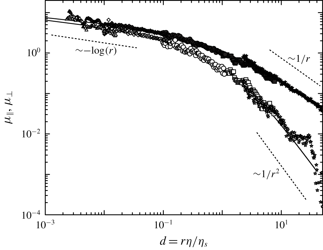
Figure 13. Mobility coefficients in the radial ( $\unicode[STIX]{x1D707}_{\Vert }$
) and azimuthal (
$\unicode[STIX]{x1D707}_{\Vert }$
) and azimuthal ( $\unicode[STIX]{x1D707}_{\bot }$
) directions (in arbitrary units) extracted from two-particle microrheology. In the surface-dominated regime (
$\unicode[STIX]{x1D707}_{\bot }$
) directions (in arbitrary units) extracted from two-particle microrheology. In the surface-dominated regime ( $Bq\gg 1$
or
$Bq\gg 1$
or $d\ll 1$
), both coefficients decay logarithmically with distance, following (3.112). In subphase-dominated cases (
$d\ll 1$
), both coefficients decay logarithmically with distance, following (3.112). In subphase-dominated cases ( $Bq\ll 1$
or
$Bq\ll 1$
or $d\gg 1$
), the coefficients decay as
$d\gg 1$
), the coefficients decay as $1/r$
and
$1/r$
and $1/r^{2}$
. The symbols correspond to two-particle displacement correlations along the line of centres (filled symbols) and perpendicular to it (empty symbols), and the solid lines are fits to (3.109). The shapes of the symbols correspond to different surface viscosities. Adapted from Prasad et al. (Reference Prasad, Koehler and Weeks2006).
$1/r^{2}$
. The symbols correspond to two-particle displacement correlations along the line of centres (filled symbols) and perpendicular to it (empty symbols), and the solid lines are fits to (3.109). The shapes of the symbols correspond to different surface viscosities. Adapted from Prasad et al. (Reference Prasad, Koehler and Weeks2006).
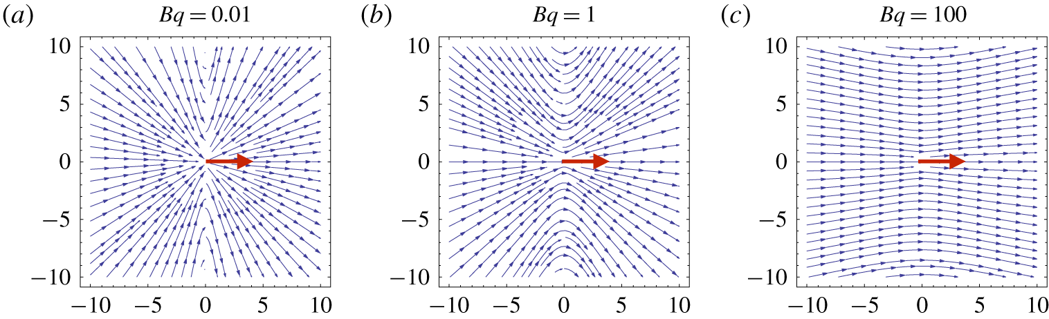
Figure 14. Streamlines of surface velocity as a result of a point force applied at the origin, following (3.108). Length is in units of $R$
such that
$R$
such that $Bq=\unicode[STIX]{x1D702}_{s}/\unicode[STIX]{x1D702}R$
.
$Bq=\unicode[STIX]{x1D702}_{s}/\unicode[STIX]{x1D702}R$
.
3.4.3 Intrinsic and apparent surface viscosity
As discussed in § 3.3, surface flows that compress or dilate the interface establish surfactant concentration gradients, generating Marangoni stresses. Surfactant exchange with the subphase returns the system to equilibrium. For small departures from equilibrium, the Marangoni stress due to a soluble surfactant (3.89) is
 $$\begin{eqnarray}-\unicode[STIX]{x1D735}_{s}\unicode[STIX]{x1D6F1}=E_{0}\unicode[STIX]{x1D70F}_{s}\unicode[STIX]{x1D735}_{s}(\unicode[STIX]{x1D735}_{s}\boldsymbol{\cdot }\boldsymbol{u}_{s}),\end{eqnarray}$$
where $E_{0}$
is the Marangoni modulus (2.22), and
$E_{0}$
is the Marangoni modulus (2.22), and $\unicode[STIX]{x1D70F}_{s}$
is the characteristic sorption time (3.56). Using (3.116) in the Boussinesq–Scriven equation (3.94) gives
$\unicode[STIX]{x1D70F}_{s}$
is the characteristic sorption time (3.56). Using (3.116) in the Boussinesq–Scriven equation (3.94) gives
 $$\begin{eqnarray}-\boldsymbol{n}\boldsymbol{\cdot }[\![\unicode[STIX]{x1D748}]\!]=\unicode[STIX]{x1D702}_{s}\unicode[STIX]{x1D6FB}_{s}^{2}\boldsymbol{u}_{s}+(E_{0}\unicode[STIX]{x1D70F}_{s}+\unicode[STIX]{x1D705}_{s})\unicode[STIX]{x1D735}_{s}(\unicode[STIX]{x1D735}_{s}\boldsymbol{\cdot }\boldsymbol{u}_{s}).\end{eqnarray}$$
As noted previously in § 3.3.2, adsorption/desorption introduces an apparent dilatational surface viscosity $\unicode[STIX]{x1D705}_{s}^{ads}=E_{0}\unicode[STIX]{x1D70F}_{s}$
. Equation (3.117) highlights the pitfalls of inferring a ‘true’ dilatational surface viscosity of a soluble surfactant. Any measurement that is sensitive to surface-viscous dissipation due to pure compression/dilatation would at best report
$\unicode[STIX]{x1D705}_{s}^{ads}=E_{0}\unicode[STIX]{x1D70F}_{s}$
. Equation (3.117) highlights the pitfalls of inferring a ‘true’ dilatational surface viscosity of a soluble surfactant. Any measurement that is sensitive to surface-viscous dissipation due to pure compression/dilatation would at best report $\unicode[STIX]{x1D705}_{s}+E_{0}\unicode[STIX]{x1D70F}_{s}$
. An intrinsic dilatational surface viscosity
$\unicode[STIX]{x1D705}_{s}+E_{0}\unicode[STIX]{x1D70F}_{s}$
. An intrinsic dilatational surface viscosity $\unicode[STIX]{x1D705}_{s}$
, should it exist, can only be established with complementary measurements of
$\unicode[STIX]{x1D705}_{s}$
, should it exist, can only be established with complementary measurements of $E_{0}$
and
$E_{0}$
and $\unicode[STIX]{x1D70F}_{s}$
.
$\unicode[STIX]{x1D70F}_{s}$
.
Furthermore, (3.117) reveals the coupling between surface shear and dilatation in one-dimensional (1-D) stretching or compression, as occurs in plate coating or thin-film drainage (§ 4.4). The 1-D version of (3.117) corresponding to deformation along the $x$
-direction is
$x$
-direction is
 $$\begin{eqnarray}\unicode[STIX]{x1D702}\left.\frac{\unicode[STIX]{x2202}v_{x}}{\unicode[STIX]{x2202}z}\right|_{z=0}=(E_{0}\unicode[STIX]{x1D70F}_{s}+\unicode[STIX]{x1D702}_{s}+\unicode[STIX]{x1D705}_{s})\frac{\unicode[STIX]{x2202}^{2}u_{s}}{\unicode[STIX]{x2202}x^{2}}.\end{eqnarray}$$
Surface-viscous dissipation in 1-D derives from a combination of surface shear viscosity, surface dilatational viscosity and the apparent viscous-like term $E_{0}\unicode[STIX]{x1D70F}_{s}$
. Surface shear viscosity inferred from such systems, therefore, is also prone to mischaracterization when
$E_{0}\unicode[STIX]{x1D70F}_{s}$
. Surface shear viscosity inferred from such systems, therefore, is also prone to mischaracterization when $E_{0}\unicode[STIX]{x1D70F}_{s}\neq 0$
. This rate- and system-dependent viscous-like contribution arising from adsorption/desorption is responsible, at least in part, for widely dissimilar values (spread over four orders of magnitude) reported for the surface viscosity of the same soluble surfactant (Stevenson Reference Stevenson2005; Zell et al.
Reference Zell, Nowbahar, Mansard, Leal, Deshmukh, Mecca, Tucker and Squires2014).
$E_{0}\unicode[STIX]{x1D70F}_{s}\neq 0$
. This rate- and system-dependent viscous-like contribution arising from adsorption/desorption is responsible, at least in part, for widely dissimilar values (spread over four orders of magnitude) reported for the surface viscosity of the same soluble surfactant (Stevenson Reference Stevenson2005; Zell et al.
Reference Zell, Nowbahar, Mansard, Leal, Deshmukh, Mecca, Tucker and Squires2014).
Non-dimensionalizing (3.118) gives
 $$\begin{eqnarray}\left.\frac{\unicode[STIX]{x2202}\tilde{v}_{x}}{\unicode[STIX]{x2202}\tilde{z}}\right|_{z=0}=\unicode[STIX]{x1D6F9}\frac{\unicode[STIX]{x2202}^{2}\tilde{u} _{s}}{\unicode[STIX]{x2202}\tilde{x}^{2}},\end{eqnarray}$$
wherein $\unicode[STIX]{x1D6F9}$
reflects a general ‘degree of immobilization’ in 1-D systems:
$\unicode[STIX]{x1D6F9}$
reflects a general ‘degree of immobilization’ in 1-D systems:
 $$\begin{eqnarray}\unicode[STIX]{x1D6F9}=\frac{(E_{0}\unicode[STIX]{x1D70F}_{s}+\unicode[STIX]{x1D702}_{s}+\unicode[STIX]{x1D705}_{s})}{\unicode[STIX]{x1D702}L}=Ma_{K}+Bq_{\unicode[STIX]{x1D702}}+Bq_{\unicode[STIX]{x1D705}}.\end{eqnarray}$$
Here, $Bq_{\unicode[STIX]{x1D702},\unicode[STIX]{x1D705}}$
are Boussinesq numbers defined separately for the intrinsic surface shear and surface dilatational viscosities. Written this way, the exchange Marangoni number
$Bq_{\unicode[STIX]{x1D702},\unicode[STIX]{x1D705}}$
are Boussinesq numbers defined separately for the intrinsic surface shear and surface dilatational viscosities. Written this way, the exchange Marangoni number $Ma_{K}=E_{0}\unicode[STIX]{x1D70F}_{s}/\unicode[STIX]{x1D702}L$
(table 3) can be interpreted as a modified Boussinesq number defined with the apparent surface dilatational viscosity,
$Ma_{K}=E_{0}\unicode[STIX]{x1D70F}_{s}/\unicode[STIX]{x1D702}L$
(table 3) can be interpreted as a modified Boussinesq number defined with the apparent surface dilatational viscosity, $\unicode[STIX]{x1D705}_{s}^{ads}=E_{0}\unicode[STIX]{x1D70F}_{s}$
, in place of an intrinsic surface viscosity.
$\unicode[STIX]{x1D705}_{s}^{ads}=E_{0}\unicode[STIX]{x1D70F}_{s}$
, in place of an intrinsic surface viscosity.
The immobilization parameter $\unicode[STIX]{x1D6F9}$
controls the transition from a stress-free interface (
$\unicode[STIX]{x1D6F9}$
controls the transition from a stress-free interface ( $\unicode[STIX]{x1D6F9}\rightarrow 0$
) to a no-slip surface (
$\unicode[STIX]{x1D6F9}\rightarrow 0$
) to a no-slip surface ( $\unicode[STIX]{x1D6F9}\rightarrow \infty$
) in 1-D compression/dilatation. In the following sections, we will see this combination appear in the contexts of settling drops, coating flows, and foams. In each of these applications, a macroscopically measurable quantity (such as the velocity of a settling drop) depends on
$\unicode[STIX]{x1D6F9}\rightarrow \infty$
) in 1-D compression/dilatation. In the following sections, we will see this combination appear in the contexts of settling drops, coating flows, and foams. In each of these applications, a macroscopically measurable quantity (such as the velocity of a settling drop) depends on $\unicode[STIX]{x1D6F9}$
in a manner that does not differentiate between
$\unicode[STIX]{x1D6F9}$
in a manner that does not differentiate between $\unicode[STIX]{x1D702}_{s}$
,
$\unicode[STIX]{x1D702}_{s}$
, $\unicode[STIX]{x1D705}_{s}$
and
$\unicode[STIX]{x1D705}_{s}$
and $E_{0}\unicode[STIX]{x1D70F}_{s}$
.
$E_{0}\unicode[STIX]{x1D70F}_{s}$
.
4 Surfactant dynamics in paradigmatic problems
Having discussed surfactant properties and their role in modifying fluid flows, we now turn to quantifying the effect of dynamic surfactant properties and processes on a series of paradigmatic problems. In particular, we will explore the motion of surfactant-covered drops and bubbles (§ 4.1), oscillatory compression of interfaces (§ 4.2), damping of surface waves (§ 4.3), coating and drainage of thin films (§ 4.4), flow through foams (§ 4.5) and particles and probes on surfactant-laden interfaces (§ 4.6). In each case, our objective is to identify the distinct ways in which the surfactant dynamics impacts measurable properties, such as the buoyant rising velocity of a bubble, the thickness of fluid entrained in dip coating or the drag on a probe translating on an interface. When possible, we quantify how each effect scales with system properties, geometries and material parameters. In so doing, we aim to connect common threads that underlie these very different systems. Perhaps more importantly, we will highlight situations where it is difficult, or even impossible, to tease apart these processes in a typical experiment. Complementary experiments might be required to unambiguously identify the ‘hidden’ surfactant and/or transport variable responsible for the observed dynamics.
4.1 Motion of surfactant-covered drops and bubbles
We will start with the ‘simple’ example that initially motivated this entire perspective – the motion of surfactant-covered drops and bubbles (figure 1). Distinct surfactant processes manifest in often indistinguishable ways, even in such a mundane flow. In this section, we will quantitatively examine the impact of surfactant variables – specifically, surface-viscous dissipation, Marangoni stresses as impacted by adsorption/desorption and surface diffusion – in modifying the motion of a drop or bubble at low Reynolds numbers (figure 15).
The translation of a rigid sphere in a viscous fluid is a classic low-Reynolds-number problem. The terminal velocity of a rigid sphere of density $\unicode[STIX]{x1D70C}^{\prime }$
and radius
$\unicode[STIX]{x1D70C}^{\prime }$
and radius $R$
settling due to its own weight (or rising due to buoyancy) through a liquid with viscosity
$R$
settling due to its own weight (or rising due to buoyancy) through a liquid with viscosity $\unicode[STIX]{x1D702}$
and density
$\unicode[STIX]{x1D702}$
and density $\unicode[STIX]{x1D70C}$
is
$\unicode[STIX]{x1D70C}$
is
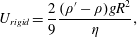 $$\begin{eqnarray}U_{rigid}=\frac{2}{9}\frac{(\unicode[STIX]{x1D70C}^{\prime }-\unicode[STIX]{x1D70C})gR^{2}}{\unicode[STIX]{x1D702}},\end{eqnarray}$$
where $g$
is the gravitational acceleration. A clean drop (or bubble) with viscosity
$g$
is the gravitational acceleration. A clean drop (or bubble) with viscosity $\unicode[STIX]{x1D702}^{\prime }$
of the same size settling (or rising) through the same liquid instead follows the Hadamard–Rybczynski formula (Levich Reference Levich1962; Happel & Brenner Reference Happel and Brenner1965)
$\unicode[STIX]{x1D702}^{\prime }$
of the same size settling (or rising) through the same liquid instead follows the Hadamard–Rybczynski formula (Levich Reference Levich1962; Happel & Brenner Reference Happel and Brenner1965)
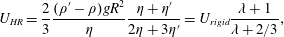 $$\begin{eqnarray}U_{HR}=\frac{2}{3}\frac{(\unicode[STIX]{x1D70C}^{\prime }-\unicode[STIX]{x1D70C})gR^{2}}{\unicode[STIX]{x1D702}}\frac{\unicode[STIX]{x1D702}+\unicode[STIX]{x1D702}^{\prime }}{2\unicode[STIX]{x1D702}+3\unicode[STIX]{x1D702}^{\prime }}=U_{rigid}\frac{\unicode[STIX]{x1D706}+1}{\unicode[STIX]{x1D706}+2/3},\end{eqnarray}$$
where
 $$\begin{eqnarray}\unicode[STIX]{x1D706}=\frac{\unicode[STIX]{x1D702}^{\prime }}{\unicode[STIX]{x1D702}}\end{eqnarray}$$
is the viscosity ratio. Equation (4.2) recovers the Stokes formula (4.1) when $\unicode[STIX]{x1D706}\gg 1$
. By contrast,
$\unicode[STIX]{x1D706}\gg 1$
. By contrast, $U_{HR}=(3/2)U_{rigid}$
when
$U_{HR}=(3/2)U_{rigid}$
when $\unicode[STIX]{x1D706}\ll 1$
, such as an air bubble rising through a viscous fluid.
$\unicode[STIX]{x1D706}\ll 1$
, such as an air bubble rising through a viscous fluid.
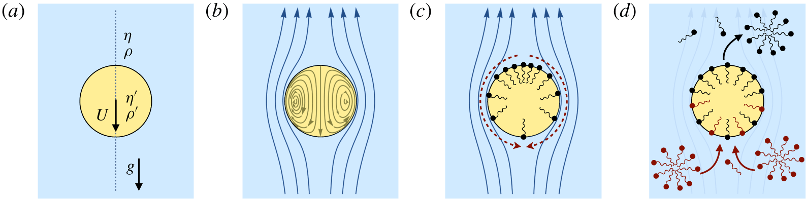
Figure 15. (a) A drop settling in a viscous fluid with terminal velocity $U$
, and (b) streamlines corresponding to the Hadamard–Rybczynski solution for a clean interface. (c) The uniform retardation regime: with adsorption–desorption or diffusion over finite time scales, a surface concentration gradient is established and a reverse Marangoni flow immobilizes the surface. (d) The remobilization regime: molecules freely desorb at the downstream pole and adsorb at the upstream pole if
$U$
, and (b) streamlines corresponding to the Hadamard–Rybczynski solution for a clean interface. (c) The uniform retardation regime: with adsorption–desorption or diffusion over finite time scales, a surface concentration gradient is established and a reverse Marangoni flow immobilizes the surface. (d) The remobilization regime: molecules freely desorb at the downstream pole and adsorb at the upstream pole if $\unicode[STIX]{x1D70F}_{s}$
is small and bulk concentration is above CMC. The resulting near-uniform surface concentration suppresses Marangoni flows and remobilizes the interface.
$\unicode[STIX]{x1D70F}_{s}$
is small and bulk concentration is above CMC. The resulting near-uniform surface concentration suppresses Marangoni flows and remobilizes the interface.
The picture changes when surfactants populate the interface between the two fluids. The interfacial boundary condition is then controlled by the interplay between convection, kinetics of adsorption/desorption, diffusion both in the bulk and on the interface and surface-viscous stresses (figure 1). Early experiments revealed discrepancies with the Hadamard–Rybczynski formula, and were attributed to impurities that modify the surface tension. In particular, Bond & Newton (Reference Bond and Newton1928) established that drops with radius under a critical value settle like rigid spheres, whereas larger drops followed (4.2). They suggested that internal circulation occurs only when the driving force (i.e. gravity) is much larger than the surface tension force, giving the critical radius $R^{2}\ll \unicode[STIX]{x1D6FE}/(\unicode[STIX]{x1D70C}^{\prime }-\unicode[STIX]{x1D70C})g$
. The well-known Bond(–Newton) number derives directly from this study. However, as we show in what follows, later studies have established that this change in the settling velocity can be attributed to dynamic surfactant processes, rather than the equilibrium surface tension.
$R^{2}\ll \unicode[STIX]{x1D6FE}/(\unicode[STIX]{x1D70C}^{\prime }-\unicode[STIX]{x1D70C})g$
. The well-known Bond(–Newton) number derives directly from this study. However, as we show in what follows, later studies have established that this change in the settling velocity can be attributed to dynamic surfactant processes, rather than the equilibrium surface tension.
4.1.1 Surface immobilization due to surface viscosity
One of the first quantitative attempts to address the inconsistency between (4.2) and measurements came from Boussinesq (Reference Boussinesq1913), who hypothesized that a thin interfacial layer provides its own ‘surface viscous’ resistance. In writing the tangential surface stress balance, Boussinesq neglected surface tension gradients and instead introduced a surface viscosity
 $$\begin{eqnarray}\boldsymbol{n}\boldsymbol{\cdot }[\![\unicode[STIX]{x1D748}]\!]\boldsymbol{\cdot }\boldsymbol{t}=\unicode[STIX]{x1D705}_{s}\boldsymbol{t}\boldsymbol{\cdot }\unicode[STIX]{x1D735}_{s}(\unicode[STIX]{x1D735}_{s}\boldsymbol{\cdot }\boldsymbol{u}_{s}).\end{eqnarray}$$
Here, $\boldsymbol{n}$
and
$\boldsymbol{n}$
and $\boldsymbol{t}$
are the normal and tangent, respectively, to the drop surface,
$\boldsymbol{t}$
are the normal and tangent, respectively, to the drop surface, $[\![\unicode[STIX]{x1D748}]\!]$
is the stress jump across the interface and
$[\![\unicode[STIX]{x1D748}]\!]$
is the stress jump across the interface and $\unicode[STIX]{x1D705}_{s}$
is an interfacial dilatational viscosity. Solving the boundary-value problem with (4.4) as the boundary condition, the terminal settling velocity of a drop is (Boussinesq Reference Boussinesq1913; Levich Reference Levich1962; Agrawal & Wasan Reference Agrawal and Wasan1979)
$\unicode[STIX]{x1D705}_{s}$
is an interfacial dilatational viscosity. Solving the boundary-value problem with (4.4) as the boundary condition, the terminal settling velocity of a drop is (Boussinesq Reference Boussinesq1913; Levich Reference Levich1962; Agrawal & Wasan Reference Agrawal and Wasan1979)
 $$\begin{eqnarray}U=U_{rigid}\frac{3\unicode[STIX]{x1D702}+3\unicode[STIX]{x1D702}^{\prime }+2\unicode[STIX]{x1D717}}{2\unicode[STIX]{x1D702}+3\unicode[STIX]{x1D702}^{\prime }+2\unicode[STIX]{x1D717}},\end{eqnarray}$$
where
 $$\begin{eqnarray}\unicode[STIX]{x1D717}=\frac{\unicode[STIX]{x1D705}_{s}}{R}\end{eqnarray}$$
is a retardation coefficient due to surface dilatational viscosity. Thus, surface viscosity has an effect analogous to increasing the effective viscosity of the drop from $\unicode[STIX]{x1D702}^{\prime }$
to
$\unicode[STIX]{x1D702}^{\prime }$
to $\unicode[STIX]{x1D702}^{\prime }+2\unicode[STIX]{x1D717}/3$
.
$\unicode[STIX]{x1D702}^{\prime }+2\unicode[STIX]{x1D717}/3$
.
The retardation coefficient $\unicode[STIX]{x1D717}$
has units of bulk shear viscosity, and can be argued based on excess energy dissipation. The energy dissipated in the drop via conventional shear viscosity scales like
$\unicode[STIX]{x1D717}$
has units of bulk shear viscosity, and can be argued based on excess energy dissipation. The energy dissipated in the drop via conventional shear viscosity scales like
 $$\begin{eqnarray}P\sim \unicode[STIX]{x1D702}^{\prime }\dot{\unicode[STIX]{x1D716}}^{2}R^{3},\end{eqnarray}$$
where $\dot{\unicode[STIX]{x1D716}}$
is the strain rate within the fluid; the dissipation per unit volume then becomes
$\dot{\unicode[STIX]{x1D716}}$
is the strain rate within the fluid; the dissipation per unit volume then becomes
 $$\begin{eqnarray}\unicode[STIX]{x1D6F7}\sim \unicode[STIX]{x1D702}^{\prime }\dot{\unicode[STIX]{x1D716}}^{2}.\end{eqnarray}$$
By extension, the retardation coefficient $\unicode[STIX]{x1D717}$
scales like the surface-excess energy
$\unicode[STIX]{x1D717}$
scales like the surface-excess energy $P_{s}$
dissipated by the surfactant, normalized by the volume of the drop
$P_{s}$
dissipated by the surfactant, normalized by the volume of the drop
 $$\begin{eqnarray}\unicode[STIX]{x1D6F7}_{s}\sim \frac{P_{s}}{R^{3}}\sim \unicode[STIX]{x1D717}\dot{\unicode[STIX]{x1D716}}^{2}.\end{eqnarray}$$
The Boussinesq number quantifies the relative strength of surface and bulk viscous stresses
 $$\begin{eqnarray}Bq_{\unicode[STIX]{x1D705}}=\frac{\unicode[STIX]{x1D717}}{\unicode[STIX]{x1D702}}=\frac{\unicode[STIX]{x1D705}_{s}}{\unicode[STIX]{x1D702}R},\end{eqnarray}$$
and the drop settling speed (4.5) can be rewritten as
 $$\begin{eqnarray}U=U_{rigid}\frac{\unicode[STIX]{x1D706}+1+2Bq_{\unicode[STIX]{x1D705}}/3}{\unicode[STIX]{x1D706}+2/3+2Bq_{\unicode[STIX]{x1D705}}/3}.\end{eqnarray}$$
Surface viscosity is negligible when $Bq_{\unicode[STIX]{x1D705}}\ll 1$
, whereas the interface is effectively immobilized and the drop behaves like a rigid sphere when surface-viscous stresses dominate (
$Bq_{\unicode[STIX]{x1D705}}\ll 1$
, whereas the interface is effectively immobilized and the drop behaves like a rigid sphere when surface-viscous stresses dominate ( $Bq_{\unicode[STIX]{x1D705}}\gg 1$
). Because
$Bq_{\unicode[STIX]{x1D705}}\gg 1$
). Because $Bq_{\unicode[STIX]{x1D705}}$
decreases as
$Bq_{\unicode[STIX]{x1D705}}$
decreases as $R$
increases, Boussinesq’s calculation reveals that bulk viscous stresses dominate over surface-viscous stresses for sufficiently large drops. For fixed
$R$
increases, Boussinesq’s calculation reveals that bulk viscous stresses dominate over surface-viscous stresses for sufficiently large drops. For fixed $\unicode[STIX]{x1D706}$
and
$\unicode[STIX]{x1D706}$
and $\unicode[STIX]{x1D705}_{s}$
, therefore, the Hadamard–Rybczynski prediction improves with an increase in drop size.
$\unicode[STIX]{x1D705}_{s}$
, therefore, the Hadamard–Rybczynski prediction improves with an increase in drop size.
4.1.2 Marangoni stress and adsorption/desorption
The Boussinesq correction due to surface viscosity does not explicitly account for the Marangoni flow associated with surface tension gradients. Levich (Reference Levich1962) accounted for convection, adsorption/desorption and diffusion in both the surface and the bulk. When drops or bubbles translate, the interfacial fluid motion advects adsorbed molecules to the rear (figure 15
c), thereby establishing a gradient in $\unicode[STIX]{x1D6E4}$
. This sets up reverse Marangoni flows, and the tangential stress balance at the interface becomes
$\unicode[STIX]{x1D6E4}$
. This sets up reverse Marangoni flows, and the tangential stress balance at the interface becomes
 $$\begin{eqnarray}\boldsymbol{n}\boldsymbol{\cdot }[\![\unicode[STIX]{x1D748}]\!]\boldsymbol{\cdot }\boldsymbol{t}=-\boldsymbol{t}\boldsymbol{\cdot }\unicode[STIX]{x1D735}_{s}\unicode[STIX]{x1D6FE}.\end{eqnarray}$$
The strength of Marangoni stresses depends on the speed with which gradients are established, compared with how quickly various processes can cause them to relax. For small departures from equilibrium surface coverage, the terminal velocity takes the same form as (4.5), but with a retardation coefficient $\unicode[STIX]{x1D717}$
that depends on the dominant surfactant transport process (Levich Reference Levich1962; Agrawal & Wasan Reference Agrawal and Wasan1979). In what follows, we outline the cases of adsorption and surface diffusion as the rate-limiting steps to illustrate the relative strength of Marangoni flows in immobilizing the interface.
$\unicode[STIX]{x1D717}$
that depends on the dominant surfactant transport process (Levich Reference Levich1962; Agrawal & Wasan Reference Agrawal and Wasan1979). In what follows, we outline the cases of adsorption and surface diffusion as the rate-limiting steps to illustrate the relative strength of Marangoni flows in immobilizing the interface.
The adsorption/desorption of soluble surfactants contributes an apparent dilatational surface viscosity (§ 3.4.3),
 $$\begin{eqnarray}\unicode[STIX]{x1D705}_{s}^{app,ads}=E_{0}\unicode[STIX]{x1D70F}_{s},\end{eqnarray}$$
where $E_{0}=\unicode[STIX]{x1D6E4}_{0}|\unicode[STIX]{x2202}\unicode[STIX]{x1D6FE}/\unicode[STIX]{x2202}\unicode[STIX]{x1D6E4}|$
is the Marangoni modulus and
$E_{0}=\unicode[STIX]{x1D6E4}_{0}|\unicode[STIX]{x2202}\unicode[STIX]{x1D6FE}/\unicode[STIX]{x2202}\unicode[STIX]{x1D6E4}|$
is the Marangoni modulus and $\unicode[STIX]{x1D70F}_{s}$
is the sorption time (3.56). The retardation coefficient in this case is identical to (4.6) but with
$\unicode[STIX]{x1D70F}_{s}$
is the sorption time (3.56). The retardation coefficient in this case is identical to (4.6) but with $\unicode[STIX]{x1D705}_{s}^{app,ads}$
in place of an intrinsic dilatational surface viscosity
$\unicode[STIX]{x1D705}_{s}^{app,ads}$
in place of an intrinsic dilatational surface viscosity $\unicode[STIX]{x1D705}_{s}$
(Levich Reference Levich1962)
$\unicode[STIX]{x1D705}_{s}$
(Levich Reference Levich1962)
 $$\begin{eqnarray}\unicode[STIX]{x1D717}_{K}=\frac{E_{0}\unicode[STIX]{x1D70F}_{s}}{R}.\end{eqnarray}$$
The drop settles at a velocity
 $$\begin{eqnarray}U=U_{rigid}\frac{\unicode[STIX]{x1D706}+1+2Ma_{K}/3}{\unicode[STIX]{x1D706}+2/3+2Ma_{K}/3},\end{eqnarray}$$
where the strength of Marangoni-induced retardation relative to bulk viscous drag defines the exchange Marangoni number (table 3)
 $$\begin{eqnarray}Ma_{K}=\frac{\unicode[STIX]{x1D717}_{K}}{\unicode[STIX]{x1D702}}=\frac{E_{0}\unicode[STIX]{x1D70F}_{s}}{\unicode[STIX]{x1D702}R}.\end{eqnarray}$$
Marangoni flows immobilize the interface ( $U\rightarrow U_{rigid}$
) when surfactant exchange with the bulk fluid is slow (
$U\rightarrow U_{rigid}$
) when surfactant exchange with the bulk fluid is slow ( $\unicode[STIX]{x1D70F}_{s}\gg \unicode[STIX]{x1D70F}_{m}=\unicode[STIX]{x1D702}R/E_{0}$
), so that
$\unicode[STIX]{x1D70F}_{s}\gg \unicode[STIX]{x1D70F}_{m}=\unicode[STIX]{x1D702}R/E_{0}$
), so that $Ma_{K}\gg 1$
. For the same fluid and surfactant properties, smaller drops (with
$Ma_{K}\gg 1$
. For the same fluid and surfactant properties, smaller drops (with $R\ll E_{0}\unicode[STIX]{x1D70F}_{s}/\unicode[STIX]{x1D702}$
) settle like rigid spheres, whereas larger drops follow the Hadamard–Rybczynski prediction.
$R\ll E_{0}\unicode[STIX]{x1D70F}_{s}/\unicode[STIX]{x1D702}$
) settle like rigid spheres, whereas larger drops follow the Hadamard–Rybczynski prediction.
As discussed in § 3.2, the time scale $\unicode[STIX]{x1D70F}_{s}$
depends on bulk diffusion gradients if exchange kinetics at the interface are sufficiently fast (
$\unicode[STIX]{x1D70F}_{s}$
depends on bulk diffusion gradients if exchange kinetics at the interface are sufficiently fast ( $\unicode[STIX]{x1D70F}_{s}\approx \unicode[STIX]{x1D70F}_{d}$
,
$\unicode[STIX]{x1D70F}_{s}\approx \unicode[STIX]{x1D70F}_{d}$
, $\unicode[STIX]{x1D70F}_{k}\approx 0$
). Additionally, if the bulk concentration
$\unicode[STIX]{x1D70F}_{k}\approx 0$
). Additionally, if the bulk concentration $C$
is above the critical micelle concentration (CMC), micelles act as surfactant reservoirs that dissociate to maintain a constant monomer concentration. As bulk concentration gradients vanish,
$C$
is above the critical micelle concentration (CMC), micelles act as surfactant reservoirs that dissociate to maintain a constant monomer concentration. As bulk concentration gradients vanish, $\unicode[STIX]{x1D70F}_{s}\approx \unicode[STIX]{x1D70F}_{d}\rightarrow 0$
, and surface concentration gradients also disappear (figure 15
d). Micelles thus act to diminish reverse Marangoni flows and reduce adsorption/desorption-based retardation by ‘remobilizing’ the interface (Stebe & Maldarelli Reference Stebe and Maldarelli1994).
$\unicode[STIX]{x1D70F}_{s}\approx \unicode[STIX]{x1D70F}_{d}\rightarrow 0$
, and surface concentration gradients also disappear (figure 15
d). Micelles thus act to diminish reverse Marangoni flows and reduce adsorption/desorption-based retardation by ‘remobilizing’ the interface (Stebe & Maldarelli Reference Stebe and Maldarelli1994).
4.1.3 Marangoni stress and surface diffusion
Diffusion of surfactant molecules on the interface can also relax surface concentration gradients, particularly when the surfactant is insoluble. Surface diffusion acts against gradients in $\unicode[STIX]{x1D6E4}$
established by surfactant advection, and the resultant profile
$\unicode[STIX]{x1D6E4}$
established by surfactant advection, and the resultant profile $\unicode[STIX]{x1D6FE}(\unicode[STIX]{x1D6E4})$
dictates the strength of the Marangoni reverse flow. Solving for a dilute system that is slightly perturbed from equilibrium, Levich (Reference Levich1962) obtained (4.5) again, but now with the retardation coefficient
$\unicode[STIX]{x1D6FE}(\unicode[STIX]{x1D6E4})$
dictates the strength of the Marangoni reverse flow. Solving for a dilute system that is slightly perturbed from equilibrium, Levich (Reference Levich1962) obtained (4.5) again, but now with the retardation coefficient
 $$\begin{eqnarray}\unicode[STIX]{x1D717}_{sd}=\frac{RE_{0}}{D_{s}},\end{eqnarray}$$
where $D_{s}$
is the surface diffusivity of the surfactant.
$D_{s}$
is the surface diffusivity of the surfactant.
This retardation coefficient captures the work dissipated as surfactant molecules are forced along the interface by chemical potential gradients. The rate of work done by a surfactant molecule of mobility $b_{s}$
forced to translate along the interface at velocity
$b_{s}$
forced to translate along the interface at velocity $U$
is
$U$
is $U^{2}/b_{s}\sim \dot{\unicode[STIX]{x1D716}}^{2}R^{2}/b_{s}$
, and the surface-excess power
$U^{2}/b_{s}\sim \dot{\unicode[STIX]{x1D716}}^{2}R^{2}/b_{s}$
, and the surface-excess power $P_{s}$
dissipated by
$P_{s}$
dissipated by ${\sim}\unicode[STIX]{x1D6E4}R^{2}$
surfactants is
${\sim}\unicode[STIX]{x1D6E4}R^{2}$
surfactants is
 $$\begin{eqnarray}P_{s}\sim \frac{\unicode[STIX]{x1D6E4}\dot{\unicode[STIX]{x1D716}}^{2}R^{4}}{b_{s}}.\end{eqnarray}$$
Following (4.9), the retardation coefficient $\unicode[STIX]{x1D717}_{sd}$
is then related to the dissipation
$\unicode[STIX]{x1D717}_{sd}$
is then related to the dissipation $\unicode[STIX]{x1D6F7}$
per unit volume of the drop,
$\unicode[STIX]{x1D6F7}$
per unit volume of the drop,
 $$\begin{eqnarray}\unicode[STIX]{x1D6F7}\sim \frac{P_{s}}{R^{3}}\sim \left(\frac{R\unicode[STIX]{x1D6E4}}{b_{s}}\right)\dot{\unicode[STIX]{x1D716}}^{2}\sim \unicode[STIX]{x1D717}_{sd}\dot{\unicode[STIX]{x1D716}}^{2}.\end{eqnarray}$$
The term within the brackets is the 3-D-viscosity-like coefficient $\unicode[STIX]{x1D717}_{sd}$
associated with dissipation in this process. In the dilute limit, the Marangoni modulus
$\unicode[STIX]{x1D717}_{sd}$
associated with dissipation in this process. In the dilute limit, the Marangoni modulus $E_{0}$
and surface concentration
$E_{0}$
and surface concentration $\unicode[STIX]{x1D6E4}$
are related via
$\unicode[STIX]{x1D6E4}$
are related via $\unicode[STIX]{x1D6E4}=E_{0}/k_{B}T$
, and the surface mobility and diffusivity are related via the Stokes–Einstein relation
$\unicode[STIX]{x1D6E4}=E_{0}/k_{B}T$
, and the surface mobility and diffusivity are related via the Stokes–Einstein relation $D_{s}=k_{B}Tb_{s}$
. Substituting
$D_{s}=k_{B}Tb_{s}$
. Substituting $\unicode[STIX]{x1D6E4}$
and
$\unicode[STIX]{x1D6E4}$
and $b$
in (4.19) recovers Levich’s form (4.17) for the retardation coefficient
$b$
in (4.19) recovers Levich’s form (4.17) for the retardation coefficient $\unicode[STIX]{x1D717}_{sd}$
.
$\unicode[STIX]{x1D717}_{sd}$
.
The surface diffusion of insoluble surfactants thus modifies the droplet settling velocity to
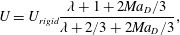 $$\begin{eqnarray}U=U_{rigid}\frac{\unicode[STIX]{x1D706}+1+2Ma_{D}/3}{\unicode[STIX]{x1D706}+2/3+2Ma_{D}/3},\end{eqnarray}$$
where the Marangoni number $Ma_{D}$
(table 3) is
$Ma_{D}$
(table 3) is
 $$\begin{eqnarray}Ma_{D}=\frac{\unicode[STIX]{x1D717}_{sd}}{\unicode[STIX]{x1D702}}=\frac{RE_{0}}{\unicode[STIX]{x1D702}D_{s}}.\end{eqnarray}$$
The interface is immobilized by reverse Marangoni flow ( $U\rightarrow U_{rigid}$
) when the surface diffusive time scale
$U\rightarrow U_{rigid}$
) when the surface diffusive time scale $R^{2}/D_{s}$
is much longer than the Marangoni time scale
$R^{2}/D_{s}$
is much longer than the Marangoni time scale $\unicode[STIX]{x1D702}R/E_{0}$
(or
$\unicode[STIX]{x1D702}R/E_{0}$
(or $Ma_{D}\gg 1$
). By contrast, the surface is mobile if
$Ma_{D}\gg 1$
). By contrast, the surface is mobile if $Ma_{D}\ll 1$
, in which case surface diffusion relaxes surface concentration gradients quickly enough that Marangoni flows do not develop.
$Ma_{D}\ll 1$
, in which case surface diffusion relaxes surface concentration gradients quickly enough that Marangoni flows do not develop.
It is tempting to express $\unicode[STIX]{x1D717}_{sd}$
from (4.17) in terms of an apparent surface viscosity, following (4.6), giving
$\unicode[STIX]{x1D717}_{sd}$
from (4.17) in terms of an apparent surface viscosity, following (4.6), giving
 $$\begin{eqnarray}\unicode[STIX]{x1D705}_{s}^{app,sd}=\frac{R^{2}E_{0}}{D_{s}}=E_{0}\unicode[STIX]{x1D70F}_{d},\end{eqnarray}$$
where $\unicode[STIX]{x1D70F}_{d}=R^{2}/D_{s}$
is the surface diffusive time scale. In this case, however, the apparent surface viscosity
$\unicode[STIX]{x1D70F}_{d}=R^{2}/D_{s}$
is the surface diffusive time scale. In this case, however, the apparent surface viscosity $\unicode[STIX]{x1D705}_{s}^{app,sd}$
depends on the size of the drop, and therefore clearly does not represent an intrinsic material property. By extension, the
$\unicode[STIX]{x1D705}_{s}^{app,sd}$
depends on the size of the drop, and therefore clearly does not represent an intrinsic material property. By extension, the $R^{2}$
dependence of
$R^{2}$
dependence of $\unicode[STIX]{x1D705}_{s}^{app,sd}$
differs from both intrinsic surface viscosity
$\unicode[STIX]{x1D705}_{s}^{app,sd}$
differs from both intrinsic surface viscosity $\unicode[STIX]{x1D705}_{s}$
and as well as the apparent
$\unicode[STIX]{x1D705}_{s}$
and as well as the apparent $\unicode[STIX]{x1D705}_{s}^{app}$
due to other dynamic surfactant processes like adsorption/desorption (4.13), suggesting experimental strategies to differentiate between the possible mechanisms.
$\unicode[STIX]{x1D705}_{s}^{app}$
due to other dynamic surfactant processes like adsorption/desorption (4.13), suggesting experimental strategies to differentiate between the possible mechanisms.
4.1.4 Inferring retardation mechanisms from measurements
The three different mechanisms of surface stress relaxation considered here – surface viscosity, Marangoni reverse flow with adsorption/desorption, and Marangoni reverse flow with surface diffusion – all lead to drop settling velocities of the form
 $$\begin{eqnarray}U=U_{rigid}\frac{\unicode[STIX]{x1D706}+1+2\unicode[STIX]{x1D6F9}/3}{\unicode[STIX]{x1D706}+2/3+2\unicode[STIX]{x1D6F9}/3}.\end{eqnarray}$$
The immobilization parameter $\unicode[STIX]{x1D6F9}$
(§ 3.4.3) acts in way that resembles an increase in the shear viscosity of the drop. The drop settles like a rigid sphere when
$\unicode[STIX]{x1D6F9}$
(§ 3.4.3) acts in way that resembles an increase in the shear viscosity of the drop. The drop settles like a rigid sphere when $\unicode[STIX]{x1D6F9}\rightarrow \infty$
, and like a clean drop when
$\unicode[STIX]{x1D6F9}\rightarrow \infty$
, and like a clean drop when $\unicode[STIX]{x1D6F9}\rightarrow 0$
. Equation (4.23) qualitatively maps out the illustrative plot in figure 1, where
$\unicode[STIX]{x1D6F9}\rightarrow 0$
. Equation (4.23) qualitatively maps out the illustrative plot in figure 1, where $\unicode[STIX]{x1D6F9}$
is determined by the ‘hidden’ surfactant variable(s). More general immobilization parameters
$\unicode[STIX]{x1D6F9}$
is determined by the ‘hidden’ surfactant variable(s). More general immobilization parameters $\unicode[STIX]{x1D6F9}=\unicode[STIX]{x1D6F9}(Ma,Pe,Da,Bq_{\unicode[STIX]{x1D705}})$
arise when surfactant transport in the bulk becomes comparable to surface processes (Levich Reference Levich1962; Agrawal & Wasan Reference Agrawal and Wasan1979), but the form of (4.23) remains unchanged. Here, the Péclet number
$\unicode[STIX]{x1D6F9}=\unicode[STIX]{x1D6F9}(Ma,Pe,Da,Bq_{\unicode[STIX]{x1D705}})$
arise when surfactant transport in the bulk becomes comparable to surface processes (Levich Reference Levich1962; Agrawal & Wasan Reference Agrawal and Wasan1979), but the form of (4.23) remains unchanged. Here, the Péclet number $Pe=UR/D$
compares advection and diffusion in the bulk, and the Damköhler number
$Pe=UR/D$
compares advection and diffusion in the bulk, and the Damköhler number $Da=k_{C}R/D$
compares adsorption to bulk diffusion.
$Da=k_{C}R/D$
compares adsorption to bulk diffusion.
Experimentally measuring drop settling velocity $U$
alone cannot reveal exactly what the surfactant does to the interface. Equation (4.23) links a measured velocity to the parameter
$U$
alone cannot reveal exactly what the surfactant does to the interface. Equation (4.23) links a measured velocity to the parameter $\unicode[STIX]{x1D6F9}$
, which could be
$\unicode[STIX]{x1D6F9}$
, which could be $Bq_{\unicode[STIX]{x1D705}}$
, some form of
$Bq_{\unicode[STIX]{x1D705}}$
, some form of $Ma$
, a function of
$Ma$
, a function of $Pe$
and
$Pe$
and $Da$
or some non-trivial combination. How can we, if at all, demarcate the specific process responsible for slowing the drop?
$Da$
or some non-trivial combination. How can we, if at all, demarcate the specific process responsible for slowing the drop?
Since one can at best measure the lumped parameter $\unicode[STIX]{x1D6F9}$
, one approach is to exploit the scaling of
$\unicode[STIX]{x1D6F9}$
, one approach is to exploit the scaling of $\unicode[STIX]{x1D6F9}$
with experimentally controllable quantities such as the bubble radius or surfactant concentration. If
$\unicode[STIX]{x1D6F9}$
with experimentally controllable quantities such as the bubble radius or surfactant concentration. If $\unicode[STIX]{x1D6F9}$
, interpreted from measurements via (4.23), increases linearly with drop size, then Marangoni flow with surface diffusion would be consistent as the dominant mechanism (
$\unicode[STIX]{x1D6F9}$
, interpreted from measurements via (4.23), increases linearly with drop size, then Marangoni flow with surface diffusion would be consistent as the dominant mechanism ( $\unicode[STIX]{x1D6F9}=Ma_{D}$
). Alternatively, if experiments suggest
$\unicode[STIX]{x1D6F9}=Ma_{D}$
). Alternatively, if experiments suggest $\unicode[STIX]{x1D6F9}\propto 1/R$
, surface viscosity (
$\unicode[STIX]{x1D6F9}\propto 1/R$
, surface viscosity ( $\unicode[STIX]{x1D6F9}=Bq_{\unicode[STIX]{x1D705}}$
), adsorption-based retardation (
$\unicode[STIX]{x1D6F9}=Bq_{\unicode[STIX]{x1D705}}$
), adsorption-based retardation ( $\unicode[STIX]{x1D6F9}=Ma_{K}$
) or both would be consistent. However, one might expect these two mechanisms to scale differently with bulk surfactant concentration
$\unicode[STIX]{x1D6F9}=Ma_{K}$
) or both would be consistent. However, one might expect these two mechanisms to scale differently with bulk surfactant concentration $C$
: an intrinsic surface viscosity
$C$
: an intrinsic surface viscosity $\unicode[STIX]{x1D705}_{s}$
likely increases with
$\unicode[STIX]{x1D705}_{s}$
likely increases with $C$
or stays constant, whereas
$C$
or stays constant, whereas $\unicode[STIX]{x1D705}_{s}^{app,ads}$
likely decreases with
$\unicode[STIX]{x1D705}_{s}^{app,ads}$
likely decreases with $C$
, since adsorptive equilibration speeds up as more surfactant is added to the bulk.
$C$
, since adsorptive equilibration speeds up as more surfactant is added to the bulk.
4.2 Oscillatory compression of soluble monolayers
The oscillatory compression of surfactant monolayers – whether in Langmuir troughs or in pulsing bubbles – provides an important method to characterize interfaces and the impact of surfactant processes on surface mechanics (Lucassen & van den Tempel Reference Lucassen and van den Tempel1972; Johnson & Stebe Reference Johnson and Stebe1994; Arriaga et al.
Reference Arriaga, López-Montero, Ignés-Mullol and Monroy2010; Ravera et al.
Reference Ravera, Loglio and Kovalchuk2010; Kotula & Anna Reference Kotula and Anna2016). The mechanical response of a dynamic interface as it is compressed depends not only on the equilibrium properties (via the isotherm) but also on the surface concentration profile $\unicode[STIX]{x1D6E4}(\boldsymbol{r}_{s},t)$
at any particular position and time. By extension, the Gibbs modulus
$\unicode[STIX]{x1D6E4}(\boldsymbol{r}_{s},t)$
at any particular position and time. By extension, the Gibbs modulus $E$
of soluble surfactants depends on the relative time scales of interfacial compression/dilatation and re-equilibration of
$E$
of soluble surfactants depends on the relative time scales of interfacial compression/dilatation and re-equilibration of $\unicode[STIX]{x1D6E4}$
. For example, during a compression so rapid that surfactants do not have time to desorb, the surface concentration must increase as
$\unicode[STIX]{x1D6E4}$
. For example, during a compression so rapid that surfactants do not have time to desorb, the surface concentration must increase as $\unicode[STIX]{x1D6E4}\sim 1/A$
, so that
$\unicode[STIX]{x1D6E4}\sim 1/A$
, so that
 $$\begin{eqnarray}E^{soluble}(t\rightarrow 0)=-A\left.\frac{\unicode[STIX]{x2202}\unicode[STIX]{x1D6F1}}{\unicode[STIX]{x2202}A}\right|_{t\rightarrow 0}\approx \unicode[STIX]{x1D6E4}\left.\frac{\unicode[STIX]{x2202}\unicode[STIX]{x1D6F1}}{\unicode[STIX]{x2202}\unicode[STIX]{x1D6E4}}\right|_{t\rightarrow 0}=E_{0}.\end{eqnarray}$$
In other words, the Gibbs modulus $E$
is equal to the Marangoni modulus
$E$
is equal to the Marangoni modulus $E_{0}$
in the rapid deformation limit. By contrast, over long enough time scales, adsorption/desorption returns
$E_{0}$
in the rapid deformation limit. By contrast, over long enough time scales, adsorption/desorption returns $\unicode[STIX]{x1D6E4}$
(and therefore
$\unicode[STIX]{x1D6E4}$
(and therefore $\unicode[STIX]{x1D6F1}$
) to its equilibrium level, so that
$\unicode[STIX]{x1D6F1}$
) to its equilibrium level, so that
 $$\begin{eqnarray}E^{soluble}(t\rightarrow \infty )=-A\left.\frac{\unicode[STIX]{x2202}\unicode[STIX]{x1D6F1}}{\unicode[STIX]{x2202}A}\right|_{\unicode[STIX]{x1D6F1}\approx const.}\approx 0\end{eqnarray}$$
for slow (or quasi-static) compression.
In general, the Gibbs modulus measured during the oscillatory compression of a soluble monolayer ranges between $0$
and
$0$
and $E_{0}$
. Moreover,
$E_{0}$
. Moreover, $\unicode[STIX]{x1D6E4}(t)$
may oscillate with some phase lag relative to the oscillating surface area
$\unicode[STIX]{x1D6E4}(t)$
may oscillate with some phase lag relative to the oscillating surface area $A$
, as discussed in § 3.2.1. Just like in shear rheology, out-of-phase responses reflect dissipative processes, meaning that the dynamic Gibbs modulus captures the apparent surface elasticity and the apparent surface dilatational viscosity, both of which depend on frequency. In what follows, we will revisit classic studies that quantified the apparent rate-dependent surface viscoelasticity originating from surfactant exchange between interface and subphase during oscillatory compression.
$A$
, as discussed in § 3.2.1. Just like in shear rheology, out-of-phase responses reflect dissipative processes, meaning that the dynamic Gibbs modulus captures the apparent surface elasticity and the apparent surface dilatational viscosity, both of which depend on frequency. In what follows, we will revisit classic studies that quantified the apparent rate-dependent surface viscoelasticity originating from surfactant exchange between interface and subphase during oscillatory compression.
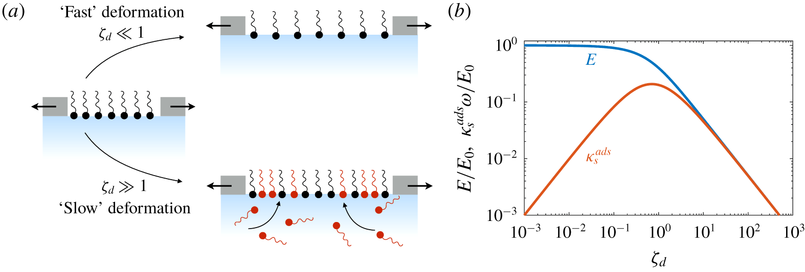
Figure 16. (a) Response of a surfactant monolayer to a dilatational deformation that is fast or slow relative to rate of replenishment by adsorption from the bulk. The monolayer is effectively insoluble as $\unicode[STIX]{x1D701}_{d}\rightarrow 0$
, and the elastic modulus is highest (
$\unicode[STIX]{x1D701}_{d}\rightarrow 0$
, and the elastic modulus is highest ( $=E_{0}$
) in this limit. Conversely, perturbations of surface concentration from equilibrium are rapidly eliminated by adsorption and the surface elasticity is weak when
$=E_{0}$
) in this limit. Conversely, perturbations of surface concentration from equilibrium are rapidly eliminated by adsorption and the surface elasticity is weak when $\unicode[STIX]{x1D701}_{d}\gg 1$
.
$\unicode[STIX]{x1D701}_{d}\gg 1$
. $(b)$
The dynamic Gibbs modulus
$(b)$
The dynamic Gibbs modulus $E$
and apparent dilatational surface viscosity
$E$
and apparent dilatational surface viscosity $\unicode[STIX]{x1D705}_{s}^{ads}$
from (4.34).
$\unicode[STIX]{x1D705}_{s}^{ads}$
from (4.34).
4.2.1 Apparent oscillatory surface rheology
Lucassen & van den Tempel (Reference Lucassen and van den Tempel1972) computed the surface pressure $\unicode[STIX]{x1D6F1}(t)$
on a planar surfactant monolayer whose area
$\unicode[STIX]{x1D6F1}(t)$
on a planar surfactant monolayer whose area $A(t)$
is forced to oscillate, and connected the monolayer response to a rate-dependent surface viscoelasticity. Figure 16 depicts the model system, consisting of a soluble monolayer at
$A(t)$
is forced to oscillate, and connected the monolayer response to a rate-dependent surface viscoelasticity. Figure 16 depicts the model system, consisting of a soluble monolayer at $z=0$
subjected to an oscillatory dilatational deformation at frequency
$z=0$
subjected to an oscillatory dilatational deformation at frequency $\unicode[STIX]{x1D714}$
(e.g. by moving barriers in a Langmuir trough), while surfactants adsorb/desorb over a time scale
$\unicode[STIX]{x1D714}$
(e.g. by moving barriers in a Langmuir trough), while surfactants adsorb/desorb over a time scale $\unicode[STIX]{x1D70F}_{s}$
.
$\unicode[STIX]{x1D70F}_{s}$
.
As discussed in § 3.2, the molecular exchange of surfactant between the surface and the subphase can be diffusion- or kinetically limited. Lucassen & van den Tempel (Reference Lucassen and van den Tempel1972) focused on the diffusion-limited regime ( $Da\gg 1$
), for which the sorption time scale
$Da\gg 1$
), for which the sorption time scale $\unicode[STIX]{x1D70F}_{s}\approx \unicode[STIX]{x1D70F}_{d}\sim L_{d}^{2}/D$
. The equilibrium surface area, surface concentration and bulk concentration fields are perturbed via
$\unicode[STIX]{x1D70F}_{s}\approx \unicode[STIX]{x1D70F}_{d}\sim L_{d}^{2}/D$
. The equilibrium surface area, surface concentration and bulk concentration fields are perturbed via
 $$\begin{eqnarray}\displaystyle & \displaystyle A(t)=A_{0}+\unicode[STIX]{x1D6FF}A\text{e}^{\text{i}\unicode[STIX]{x1D714}t}, & \displaystyle\end{eqnarray}$$
 $$\begin{eqnarray}\displaystyle & \displaystyle \unicode[STIX]{x1D6E4}(t)=\unicode[STIX]{x1D6E4}_{0}+\unicode[STIX]{x1D6FF}\unicode[STIX]{x1D6E4}\text{e}^{\text{i}\unicode[STIX]{x1D714}t}, & \displaystyle\end{eqnarray}$$
 $$\begin{eqnarray}\displaystyle & \displaystyle C(z,t)=C_{0}+\unicode[STIX]{x1D6FF}C\text{e}^{\text{i}(\unicode[STIX]{x1D714}t+kz)}, & \displaystyle\end{eqnarray}$$ $z<0$
). The bulk concentration
$z<0$
). The bulk concentration $C$
satisfies the diffusion equation (3.26), with solution
$C$
satisfies the diffusion equation (3.26), with solution  $$\begin{eqnarray}k=(1-\text{i})\sqrt{\frac{\unicode[STIX]{x1D714}}{2D}}.\end{eqnarray}$$
Both real and imaginary components of $\unicode[STIX]{x1D6FF}\unicode[STIX]{x1D6E4}$
resist interfacial dilatation, and a convenient measure of the net resistance is the complex dilatational modulus
$\unicode[STIX]{x1D6FF}\unicode[STIX]{x1D6E4}$
resist interfacial dilatation, and a convenient measure of the net resistance is the complex dilatational modulus
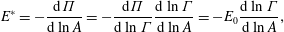 $$\begin{eqnarray}E^{\ast }=-\frac{\text{d}\unicode[STIX]{x1D6F1}}{\text{d}\ln A}=-\frac{\text{d}\unicode[STIX]{x1D6F1}}{\text{d}\ln \unicode[STIX]{x1D6E4}}\frac{\text{d}\ln \unicode[STIX]{x1D6E4}}{\text{d}\ln A}=-E_{0}\frac{\text{d}\ln \unicode[STIX]{x1D6E4}}{\text{d}\ln A},\end{eqnarray}$$
where $E_{0}=\text{d}\unicode[STIX]{x1D6F1}/\text{d}\ln \unicode[STIX]{x1D6E4}$
is the Marangoni modulus (§ 2.4.2). We will assume that
$E_{0}=\text{d}\unicode[STIX]{x1D6F1}/\text{d}\ln \unicode[STIX]{x1D6E4}$
is the Marangoni modulus (§ 2.4.2). We will assume that $\unicode[STIX]{x1D6F1}(t)$
is in phase with and uniquely determined by
$\unicode[STIX]{x1D6F1}(t)$
is in phase with and uniquely determined by $\unicode[STIX]{x1D6E4}(t)$
, so that
$\unicode[STIX]{x1D6E4}(t)$
, so that $E_{0}$
is independent of
$E_{0}$
is independent of $\unicode[STIX]{x1D714}$
. Note, however, that
$\unicode[STIX]{x1D714}$
. Note, however, that $\unicode[STIX]{x1D6E4}$
and
$\unicode[STIX]{x1D6E4}$
and $A$
may not vary precisely in phase: even monolayers of insoluble surfactant monolayers may relax to equilibrium over surprisingly long times, as discussed in § 5. Surfactant transport thus affects
$A$
may not vary precisely in phase: even monolayers of insoluble surfactant monolayers may relax to equilibrium over surprisingly long times, as discussed in § 5. Surfactant transport thus affects $E^{\ast }$
via the dynamic behaviour of
$E^{\ast }$
via the dynamic behaviour of $\unicode[STIX]{x1D6E4}(A)$
in (4.28). The real part of
$\unicode[STIX]{x1D6E4}(A)$
in (4.28). The real part of $E^{\ast }$
is the dynamic Gibbs modulus, whereas the imaginary or out-of-phase component captures the viscous-like dissipation associated with surfactant exchange.
$E^{\ast }$
is the dynamic Gibbs modulus, whereas the imaginary or out-of-phase component captures the viscous-like dissipation associated with surfactant exchange.
Surfactant conservation at the interface with diffusion-limited adsorption (§ 3.2) requires
 $$\begin{eqnarray}\frac{1}{A}\frac{\unicode[STIX]{x2202}(\unicode[STIX]{x1D6E4}A)}{\unicode[STIX]{x2202}t}=j_{diff}=-D\left.\frac{\unicode[STIX]{x2202}C}{\unicode[STIX]{x2202}z}\right|_{z=0}.\end{eqnarray}$$
Contact equilibrium is assumed between the surface concentration $\unicode[STIX]{x1D6E4}(t)$
and the bulk concentration
$\unicode[STIX]{x1D6E4}(t)$
and the bulk concentration $C_{s}(t)=C(0,t)$
when diffusion controlled, so that
$C_{s}(t)=C(0,t)$
when diffusion controlled, so that
 $$\begin{eqnarray}\frac{1}{A}\frac{\unicode[STIX]{x2202}(\unicode[STIX]{x1D6E4}A)}{\unicode[STIX]{x2202}t}=\left(1+\frac{\unicode[STIX]{x2202}\ln A}{\unicode[STIX]{x2202}\ln \unicode[STIX]{x1D6E4}}\right)\frac{\unicode[STIX]{x2202}\unicode[STIX]{x1D6E4}}{\unicode[STIX]{x2202}t}=\left(1+\frac{\unicode[STIX]{x2202}\ln A}{\unicode[STIX]{x2202}\ln \unicode[STIX]{x1D6E4}}\right)L_{p}\left.\frac{\unicode[STIX]{x2202}C}{\unicode[STIX]{x2202}t}\right|_{z=0},\end{eqnarray}$$
where $L_{p}=\unicode[STIX]{x2202}\unicode[STIX]{x1D6E4}/\unicode[STIX]{x2202}C_{s}$
is the depletion depth (3.47). Using (4.30) in (4.29) gives
$L_{p}=\unicode[STIX]{x2202}\unicode[STIX]{x1D6E4}/\unicode[STIX]{x2202}C_{s}$
is the depletion depth (3.47). Using (4.30) in (4.29) gives
 $$\begin{eqnarray}\frac{\unicode[STIX]{x2202}\ln \unicode[STIX]{x1D6E4}}{\unicode[STIX]{x2202}\ln A}=-\left(1+\frac{D}{L_{d}}\frac{\unicode[STIX]{x2202}C/\unicode[STIX]{x2202}z|_{z=0}}{\unicode[STIX]{x2202}C/\unicode[STIX]{x2202}t|_{z=0}}\right)^{-1}.\end{eqnarray}$$
Substituting perturbed variables (4.26) in (4.31) then gives the complex modulus (4.28):
 $$\begin{eqnarray}E^{\ast }=\frac{E_{0}}{1+\unicode[STIX]{x1D701}_{d}-\text{i}\unicode[STIX]{x1D701}_{d}},\end{eqnarray}$$
where
 $$\begin{eqnarray}\unicode[STIX]{x1D701}_{d}=\frac{1}{L_{d}}\sqrt{\frac{D}{2\unicode[STIX]{x1D714}}}\end{eqnarray}$$
is a dimensionless ratio of the diffusive boundary layer thickness $\unicode[STIX]{x1D6FF}_{BL}=\sqrt{D/2\unicode[STIX]{x1D714}}$
to the depletion depth
$\unicode[STIX]{x1D6FF}_{BL}=\sqrt{D/2\unicode[STIX]{x1D714}}$
to the depletion depth $L_{p}=\unicode[STIX]{x2202}\unicode[STIX]{x1D6E4}/\unicode[STIX]{x2202}C_{s}$
, first introduced as (3.51) in § 3.2.
$L_{p}=\unicode[STIX]{x2202}\unicode[STIX]{x1D6E4}/\unicode[STIX]{x2202}C_{s}$
, first introduced as (3.51) in § 3.2.
The apparent surface-elastic and surface-viscous moduli are the real and imaginary parts of $E^{\ast }$
, respectively
$E^{\ast }$
, respectively
 $$\begin{eqnarray}\displaystyle & \displaystyle E=\text{Re}[E^{\ast }]=E_{0}\frac{1+\unicode[STIX]{x1D701}_{d}}{1+2\unicode[STIX]{x1D701}_{d}+2\unicode[STIX]{x1D701}_{d}^{2}}, & \displaystyle\end{eqnarray}$$
 $$\begin{eqnarray}\displaystyle & \displaystyle \unicode[STIX]{x1D705}_{s}^{ads}=\frac{\text{Im}[E^{\ast }]}{\unicode[STIX]{x1D714}}=\frac{E_{0}}{\unicode[STIX]{x1D714}}\frac{\unicode[STIX]{x1D701}_{d}}{1+2\unicode[STIX]{x1D701}_{d}+2\unicode[STIX]{x1D701}_{d}^{2}}. & \displaystyle\end{eqnarray}$$ $\unicode[STIX]{x1D701}_{d}\ll 1$
), surfactant molecules do not diffusively escape the depletion depth before the barrier reverses direction, so the interface behaves as insoluble, with
$\unicode[STIX]{x1D701}_{d}\ll 1$
), surfactant molecules do not diffusively escape the depletion depth before the barrier reverses direction, so the interface behaves as insoluble, with $E\rightarrow E_{0}$
. By contrast, during ‘slow’ oscillations (
$E\rightarrow E_{0}$
. By contrast, during ‘slow’ oscillations ( $\unicode[STIX]{x1D701}_{d}\gg 1$
), the oscillatory boundary layer is thicker than the depletion depth (
$\unicode[STIX]{x1D701}_{d}\gg 1$
), the oscillatory boundary layer is thicker than the depletion depth ( $\unicode[STIX]{x1D6FF}_{BL}\gg L_{p}$
). In this limit, dissolved molecules diffuse across the depletion depth during each oscillation and restore the sublayer concentration to
$\unicode[STIX]{x1D6FF}_{BL}\gg L_{p}$
). In this limit, dissolved molecules diffuse across the depletion depth during each oscillation and restore the sublayer concentration to $C_{0}$
before the barrier reverses. Molecules then adsorb/desorb much more quickly than the interface is compressed and dilatated, so that
$C_{0}$
before the barrier reverses. Molecules then adsorb/desorb much more quickly than the interface is compressed and dilatated, so that $\unicode[STIX]{x1D6E4}(t)\approx \unicode[STIX]{x1D6E4}_{0}$
and the Gibbs modulus vanishes. The apparent dilatational surface viscosity
$\unicode[STIX]{x1D6E4}(t)\approx \unicode[STIX]{x1D6E4}_{0}$
and the Gibbs modulus vanishes. The apparent dilatational surface viscosity $\unicode[STIX]{x1D705}_{s}^{ads}$
is highest when
$\unicode[STIX]{x1D705}_{s}^{ads}$
is highest when $\unicode[STIX]{x1D701}_{d}=O(1)$
, i.e. when
$\unicode[STIX]{x1D701}_{d}=O(1)$
, i.e. when $\unicode[STIX]{x1D70F}_{\unicode[STIX]{x1D714}}\sim \unicode[STIX]{x1D70F}_{d}$
.
$\unicode[STIX]{x1D70F}_{\unicode[STIX]{x1D714}}\sim \unicode[STIX]{x1D70F}_{d}$
.
More generally, the complex dilatational modulus $E^{\ast }$
depends on the Damköhler number
$E^{\ast }$
depends on the Damköhler number $Da$
(3.40). We will generalize
$Da$
(3.40). We will generalize $E^{\ast }$
for finite
$E^{\ast }$
for finite $Da$
and non-planar interfaces in the next section, but simply note that the qualitative trends of
$Da$
and non-planar interfaces in the next section, but simply note that the qualitative trends of $E^{\ast }$
resemble those in figure 16(b), regardless of system geometry:
$E^{\ast }$
resemble those in figure 16(b), regardless of system geometry: $|E^{\ast }|\rightarrow E_{0}$
for slow adsorption/desorption (or rapid deformation), and
$|E^{\ast }|\rightarrow E_{0}$
for slow adsorption/desorption (or rapid deformation), and $|E|\rightarrow 0$
for slow deformations.
$|E|\rightarrow 0$
for slow deformations.
4.2.2 Oscillating bubble tensiometry
Oscillating bubbles make excellent experimental probes of dilatational surface rheology (Ravera et al. Reference Ravera, Loglio and Kovalchuk2010; Kotula & Anna Reference Kotula and Anna2016). Indeed, § 3.2.1 illustrated kinetically and diffusion-limited surfactant exchange via oscillating bubbles. Here, we will follow Johnson & Stebe (Reference Johnson and Stebe1994) in examining the surface stresses that arise in oscillating bubbles, how they depend on adsorption/desorption, surface rheology and the subphase viscosity.
Alvarez et al. (Reference Alvarez, Walker and Anna2010a
) developed a microbubble microtensiometer, which simultaneously measures the radius and gas pressure of $O(100~\unicode[STIX]{x03BC}\text{m})$
bubbles. For a static bubble with equilibrated surface coverage, the surface tension (or surface pressure) is then determined via the Young–Laplace equation (2.6). Indeed, the equilibrium isotherm of insoluble monolayers can be mapped out by quasi-static compression of a spherical bubble (Kotula & Anna Reference Kotula and Anna2016).
$O(100~\unicode[STIX]{x03BC}\text{m})$
bubbles. For a static bubble with equilibrated surface coverage, the surface tension (or surface pressure) is then determined via the Young–Laplace equation (2.6). Indeed, the equilibrium isotherm of insoluble monolayers can be mapped out by quasi-static compression of a spherical bubble (Kotula & Anna Reference Kotula and Anna2016).
To quantify the impact of surfactant adsorption/desorption, mass transport and surface rheology on dynamic bubbles, we return to the work of Johnson & Stebe (Reference Johnson and Stebe1994), first introduced in § 3.2.1, involving an oscillating air bubble of radius $R(t)$
, with dynamic surface concentration
$R(t)$
, with dynamic surface concentration $\unicode[STIX]{x1D6E4}(t)$
, in a liquid containing dissolved surfactant at concentration
$\unicode[STIX]{x1D6E4}(t)$
, in a liquid containing dissolved surfactant at concentration $C(t)$
. Fluid pressure and radial velocity in both gas and liquid phases are perturbed as before (3.29), via
$C(t)$
. Fluid pressure and radial velocity in both gas and liquid phases are perturbed as before (3.29), via
 $$\begin{eqnarray}v_{r}(r,t)=\unicode[STIX]{x1D6FF}v_{r}(r)\text{e}^{\text{i}\unicode[STIX]{x1D714}t},\quad p(r,t)=p_{0}+\unicode[STIX]{x1D6FF}p(r)\text{e}^{\text{i}\unicode[STIX]{x1D714}t}.\end{eqnarray}$$
Solving the unsteady Stokes equations gives
 $$\begin{eqnarray}\displaystyle & \displaystyle \unicode[STIX]{x1D6FF}v(r)=\frac{\text{i}\unicode[STIX]{x1D714}R_{0}^{2}}{r^{2}}\unicode[STIX]{x1D6FF}R, & \displaystyle\end{eqnarray}$$
 $$\begin{eqnarray}\displaystyle & \displaystyle \unicode[STIX]{x1D6FF}p(r)=-\frac{\unicode[STIX]{x1D70C}\unicode[STIX]{x1D714}^{2}R_{0}^{2}}{r}\unicode[STIX]{x1D6FF}R, & \displaystyle\end{eqnarray}$$
Assuming the gas viscosity to be negligible, the gas pressure is uniform throughout the bubble ( $p_{g}=p_{g}(R)$
) and is determined by the stress balance at the interface (3.8). Assuming also that the adsorbed surfactant forms a Newtonian monolayer and simplifying the Boussinesq–Scriven stress tensor (3.93) for radial deformation gives (Scriven Reference Scriven1960):
$p_{g}=p_{g}(R)$
) and is determined by the stress balance at the interface (3.8). Assuming also that the adsorbed surfactant forms a Newtonian monolayer and simplifying the Boussinesq–Scriven stress tensor (3.93) for radial deformation gives (Scriven Reference Scriven1960):
 $$\begin{eqnarray}p_{g}-p_{l}(R)+2\unicode[STIX]{x1D702}\left.\frac{\unicode[STIX]{x2202}v_{r}}{\unicode[STIX]{x2202}r}\right|_{r=R}=\frac{2\unicode[STIX]{x1D6FE}}{R}+\frac{4\unicode[STIX]{x1D705}_{s}v_{r}(R)}{R^{2}}.\end{eqnarray}$$
The perturbed surface tension is
 $$\begin{eqnarray}\unicode[STIX]{x1D6FE}=\unicode[STIX]{x1D6FE}(\unicode[STIX]{x1D6E4}_{0})+\left.\frac{\unicode[STIX]{x2202}\unicode[STIX]{x1D6FE}}{\unicode[STIX]{x2202}\unicode[STIX]{x1D6E4}}\right|_{\unicode[STIX]{x1D6E4}_{0}}\unicode[STIX]{x1D6FF}\unicode[STIX]{x1D6E4}\text{e}^{\text{i}\unicode[STIX]{x1D714}t}=\unicode[STIX]{x1D6FE}_{0}-\frac{E_{0}}{\unicode[STIX]{x1D6E4}_{0}}\unicode[STIX]{x1D6FF}\unicode[STIX]{x1D6E4}\text{e}^{\text{i}\unicode[STIX]{x1D714}t},\end{eqnarray}$$
so that the leading-order interfacial stress balance (4.37) is the Young–Laplace equation
 $$\begin{eqnarray}p_{g,0}-p_{l,0}(R_{0})=\frac{2\unicode[STIX]{x1D6FE}_{0}}{R_{0}}.\end{eqnarray}$$
At $O(\unicode[STIX]{x1D6FF}R)$
, however, the pressure jump at the interface has contributions due to Young–Laplace from the radial change, the resistance to dilatation due to changes in adsorbed surfactant concentration (and therefore
$O(\unicode[STIX]{x1D6FF}R)$
, however, the pressure jump at the interface has contributions due to Young–Laplace from the radial change, the resistance to dilatation due to changes in adsorbed surfactant concentration (and therefore $\unicode[STIX]{x1D6F1}$
), the viscous resistance from the bulk liquid and dilatational surface viscous resistance
$\unicode[STIX]{x1D6F1}$
), the viscous resistance from the bulk liquid and dilatational surface viscous resistance
 $$\begin{eqnarray}\unicode[STIX]{x1D6FF}p_{g}-\unicode[STIX]{x1D6FF}p_{l}(R)=\left[-\frac{2\unicode[STIX]{x1D6FE}_{0}}{R_{0}^{2}}+\frac{4E_{0}}{R_{0}^{2}}\frac{\unicode[STIX]{x1D6FF}\unicode[STIX]{x1D6E4}}{\unicode[STIX]{x1D6FF}\unicode[STIX]{x1D6E4}_{insol}}+\frac{4\text{i}\unicode[STIX]{x1D714}\unicode[STIX]{x1D702}}{R_{0}}+\frac{4\text{i}\unicode[STIX]{x1D714}\unicode[STIX]{x1D705}_{s}}{R_{0}^{2}}\right]\unicode[STIX]{x1D6FF}R,\end{eqnarray}$$
where
 $$\begin{eqnarray}\unicode[STIX]{x1D6FF}\unicode[STIX]{x1D6E4}_{insol}=-2\unicode[STIX]{x1D6E4}_{0}\frac{\unicode[STIX]{x1D6FF}R}{R_{0}}\end{eqnarray}$$
is the surface concentration change in the insoluble limit (3.32). Recall from § 3.2.1 that $\unicode[STIX]{x1D6FF}\unicode[STIX]{x1D6E4}$
in (4.40) is complex, with components both in and out of phase with
$\unicode[STIX]{x1D6FF}\unicode[STIX]{x1D6E4}$
in (4.40) is complex, with components both in and out of phase with $\unicode[STIX]{x1D6FF}R$
.
$\unicode[STIX]{x1D6FF}R$
.
Non-dimensionalizing length and pressure in (4.40) using $R_{0}$
and the Laplace pressure
$R_{0}$
and the Laplace pressure $2\unicode[STIX]{x1D6FE}_{0}/R_{0}$
respectively gives
$2\unicode[STIX]{x1D6FE}_{0}/R_{0}$
respectively gives
 $$\begin{eqnarray}\unicode[STIX]{x1D6FF}\tilde{p}_{g}-\unicode[STIX]{x1D6FF}\tilde{p}_{l}(R)=\unicode[STIX]{x1D712}\unicode[STIX]{x1D6FF}\tilde{R},\end{eqnarray}$$
where
 $$\begin{eqnarray}\unicode[STIX]{x1D712}=-1+2Ma_{\unicode[STIX]{x1D6FE}}\frac{\text{Re}[\unicode[STIX]{x1D6FF}\unicode[STIX]{x1D6E4}]}{\unicode[STIX]{x1D6FF}\unicode[STIX]{x1D6E4}_{insol}}+2\text{i}Ca\left(1+Bq_{\unicode[STIX]{x1D705}}+Ma\frac{\text{Im}[\unicode[STIX]{x1D6FF}\unicode[STIX]{x1D6E4}]}{\unicode[STIX]{x1D6FF}\unicode[STIX]{x1D6E4}_{insol}}\right)\end{eqnarray}$$
and the capillary, Marangoni and Boussinesq numbers are
 $$\begin{eqnarray}Ca=\frac{\unicode[STIX]{x1D702}R_{0}\unicode[STIX]{x1D714}}{\unicode[STIX]{x1D6FE}_{0}},\quad Ma=\frac{E_{0}}{\unicode[STIX]{x1D702}R_{0}\unicode[STIX]{x1D714}},\quad Ma_{\unicode[STIX]{x1D6FE}}=Ma\times Ca=\frac{E_{0}}{\unicode[STIX]{x1D6FE}},\quad Bq_{\unicode[STIX]{x1D705}}=\frac{\unicode[STIX]{x1D705}_{s}}{\unicode[STIX]{x1D702}R_{0}}.\end{eqnarray}$$
Evaluating (4.42)–(4.44) requires the solution for $\unicode[STIX]{x1D6FF}\unicode[STIX]{x1D6E4}/\unicode[STIX]{x1D6FF}\unicode[STIX]{x1D6E4}_{insol}$
, described in § 3.2.1 and given by (3.41) and reproduced here
$\unicode[STIX]{x1D6FF}\unicode[STIX]{x1D6E4}/\unicode[STIX]{x1D6FF}\unicode[STIX]{x1D6E4}_{insol}$
, described in § 3.2.1 and given by (3.41) and reproduced here
 $$\begin{eqnarray}\frac{\unicode[STIX]{x1D6FF}\unicode[STIX]{x1D6E4}}{\unicode[STIX]{x1D6FF}\unicode[STIX]{x1D6E4}_{insol}}=\left[1-\text{i}\,St\left(\frac{1+\sqrt{\text{i}Wo}}{1+\sqrt{\text{i}Wo}+Da}\right)\right]^{-1},\end{eqnarray}$$
where the Stanton, Womersley and Damköhler numbers are
 $$\begin{eqnarray}St=\frac{k_{\unicode[STIX]{x1D6E4}}}{\unicode[STIX]{x1D714}},\quad Wo=\frac{\unicode[STIX]{x1D714}R_{0}^{2}}{D},\quad \text{and}\quad Da=\frac{k_{C}R_{0}}{D}.\end{eqnarray}$$
Surfactant-free bubbles lack surface-viscous and surface-elastic stresses ( $Ma=Bq_{\unicode[STIX]{x1D705}}=0$
). The interfacial stress balance (4.42) then recovers the linear limit of the classic Rayleigh–Plesset equation (Marmottant et al.
Reference Marmottant, van der Meer, Emmer, Versluis, de Jong, Hilgenfeldt and Lohse2005)
$Ma=Bq_{\unicode[STIX]{x1D705}}=0$
). The interfacial stress balance (4.42) then recovers the linear limit of the classic Rayleigh–Plesset equation (Marmottant et al.
Reference Marmottant, van der Meer, Emmer, Versluis, de Jong, Hilgenfeldt and Lohse2005)
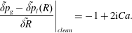 $$\begin{eqnarray}\left.\frac{\tilde{\unicode[STIX]{x1D6FF}p}_{g}-\tilde{\unicode[STIX]{x1D6FF}p}_{l}(R)}{\tilde{\unicode[STIX]{x1D6FF}R}}\right|_{clean}=-1+2\text{i}Ca.\end{eqnarray}$$
The normal stress jump balances the perturbed Laplace pressure due to change in radius and the viscous stress from the liquid phase.
Bubbles with insoluble surfactants have surface concentrations that change in phase with the oscillations, giving $\text{Re}[\unicode[STIX]{x1D6FF}\unicode[STIX]{x1D6E4}]=\unicode[STIX]{x1D6FF}\unicode[STIX]{x1D6E4}_{insol}$
and
$\text{Re}[\unicode[STIX]{x1D6FF}\unicode[STIX]{x1D6E4}]=\unicode[STIX]{x1D6FF}\unicode[STIX]{x1D6E4}_{insol}$
and $\text{Im}[\unicode[STIX]{x1D6FF}\unicode[STIX]{x1D6E4}]=0$
, so that (4.42) becomes
$\text{Im}[\unicode[STIX]{x1D6FF}\unicode[STIX]{x1D6E4}]=0$
, so that (4.42) becomes
 $$\begin{eqnarray}\left.\frac{\tilde{\unicode[STIX]{x1D6FF}p}_{g}-\tilde{\unicode[STIX]{x1D6FF}p}_{l}(R)}{\tilde{\unicode[STIX]{x1D6FF}R}}\right|_{insol}=-1+2Ma_{\unicode[STIX]{x1D6FE}}+2\text{i}Ca+2\text{i}Bq_{\unicode[STIX]{x1D705}}Ca.\end{eqnarray}$$
The pressure jump across the interface then balances additional surface stresses: the terms proportional to $Ma_{\unicode[STIX]{x1D6FE}}$
and
$Ma_{\unicode[STIX]{x1D6FE}}$
and $Bq_{\unicode[STIX]{x1D705}}Ca$
quantify the elastic and intrinsic surface-viscous resistance to interfacial dilatation/compression, respectively.
$Bq_{\unicode[STIX]{x1D705}}Ca$
quantify the elastic and intrinsic surface-viscous resistance to interfacial dilatation/compression, respectively.
Surface-elastic resistance to bubble expansion decreases for soluble surfactants, however, since adsorption/desorption diminishes perturbations to surface concentration, and $\text{Re}[\unicode[STIX]{x1D6FF}\unicode[STIX]{x1D6E4}]<\unicode[STIX]{x1D6FF}\unicode[STIX]{x1D6E4}_{insol}$
. Solubility also introduces an out-of-phase component of surface concentration, so that
$\text{Re}[\unicode[STIX]{x1D6FF}\unicode[STIX]{x1D6E4}]<\unicode[STIX]{x1D6FF}\unicode[STIX]{x1D6E4}_{insol}$
. Solubility also introduces an out-of-phase component of surface concentration, so that $\text{Im}[\unicode[STIX]{x1D6FF}\unicode[STIX]{x1D6E4}]\neq 0$
, giving rise to an additional surface-viscous-like stress as in § 4.2.1.
$\text{Im}[\unicode[STIX]{x1D6FF}\unicode[STIX]{x1D6E4}]\neq 0$
, giving rise to an additional surface-viscous-like stress as in § 4.2.1.
The dynamic Gibbs modulus $E$
and the apparent dilatational surface viscosity
$E$
and the apparent dilatational surface viscosity $\unicode[STIX]{x1D705}_{s}^{ads}$
are the real and imaginary parts of the complex modulus
$\unicode[STIX]{x1D705}_{s}^{ads}$
are the real and imaginary parts of the complex modulus $E^{\ast }$
(§ 4.2.1). For small oscillatory perturbations around a spherical bubble, (4.28) gives
$E^{\ast }$
(§ 4.2.1). For small oscillatory perturbations around a spherical bubble, (4.28) gives
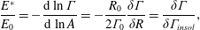 $$\begin{eqnarray}\frac{E^{\ast }}{E_{0}}=-\frac{\text{d}\ln \unicode[STIX]{x1D6E4}}{\text{d}\ln A}=-\frac{R_{0}}{2\unicode[STIX]{x1D6E4}_{0}}\frac{\unicode[STIX]{x1D6FF}\unicode[STIX]{x1D6E4}}{\unicode[STIX]{x1D6FF}R}=\frac{\unicode[STIX]{x1D6FF}\unicode[STIX]{x1D6E4}}{\unicode[STIX]{x1D6FF}\unicode[STIX]{x1D6E4}_{insol}},\end{eqnarray}$$
so that using (4.45) for $\unicode[STIX]{x1D6FF}\unicode[STIX]{x1D6E4}$
gives
$\unicode[STIX]{x1D6FF}\unicode[STIX]{x1D6E4}$
gives
 $$\begin{eqnarray}\frac{E^{\ast }}{E_{0}}=\left[1-\text{i}\,St\left(\frac{1+\sqrt{\text{i}\,Wo}}{1+\sqrt{\text{i}\,Wo}+Da}\right)\right]^{-1}.\end{eqnarray}$$
Surfactant exchange between the interface and subphase is kinetically limited when the bulk diffusion time $\unicode[STIX]{x1D70F}_{d}$
is much smaller than the kinetic time
$\unicode[STIX]{x1D70F}_{d}$
is much smaller than the kinetic time $\unicode[STIX]{x1D70F}_{k}$
(see § 3.2.1). In the kinetically limited (
$\unicode[STIX]{x1D70F}_{k}$
(see § 3.2.1). In the kinetically limited ( $Da=\unicode[STIX]{x1D70F}_{d}/\unicode[STIX]{x1D70F}_{k}\rightarrow 0$
) case, (4.50) becomes
$Da=\unicode[STIX]{x1D70F}_{d}/\unicode[STIX]{x1D70F}_{k}\rightarrow 0$
) case, (4.50) becomes
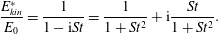 $$\begin{eqnarray}\frac{E_{kin}^{\ast }}{E_{0}}=\frac{1}{1-\text{i}St}=\frac{1}{1+St^{2}}+\text{i}\frac{St}{1+St^{2}}.\end{eqnarray}$$
The monolayer is effectively insoluble, and the Gibbs modulus $E$
approaches the Marangoni modulus
$E$
approaches the Marangoni modulus $E_{0}$
, in the limit that adsorption kinetics are so slow that
$E_{0}$
, in the limit that adsorption kinetics are so slow that $\unicode[STIX]{x1D6E4}(t)$
does not change appreciably before the oscillatory cycle reverses (or
$\unicode[STIX]{x1D6E4}(t)$
does not change appreciably before the oscillatory cycle reverses (or $St\rightarrow 0$
). By contrast,
$St\rightarrow 0$
). By contrast, $\unicode[STIX]{x1D6E4}(t)$
is approximately constant if adsorption/desorption is fast relative to bubble oscillations (
$\unicode[STIX]{x1D6E4}(t)$
is approximately constant if adsorption/desorption is fast relative to bubble oscillations ( $St\rightarrow \infty$
), so that the monolayer provides no resistance to compression/dilatation. Bubble size does not affect
$St\rightarrow \infty$
), so that the monolayer provides no resistance to compression/dilatation. Bubble size does not affect $E_{kin}^{\ast }$
when transport is kinetically limited: the oscillatory mechanical response of a soluble planar monolayer (§ 4.2.1) also follows (4.51) in the kinetically limited regime
$E_{kin}^{\ast }$
when transport is kinetically limited: the oscillatory mechanical response of a soluble planar monolayer (§ 4.2.1) also follows (4.51) in the kinetically limited regime $Da\rightarrow 0$
.
$Da\rightarrow 0$
.
Alternatively, adsorption is diffusion limited when $\unicode[STIX]{x1D70F}_{d}\gg \unicode[STIX]{x1D70F}_{k}$
(or
$\unicode[STIX]{x1D70F}_{d}\gg \unicode[STIX]{x1D70F}_{k}$
(or $Da\gg 1$
), and surface concentration rapidly equilibrates with the subsurface concentration
$Da\gg 1$
), and surface concentration rapidly equilibrates with the subsurface concentration $C_{s}(t)=C(R,t)$
via an isotherm
$C_{s}(t)=C(R,t)$
via an isotherm $\unicode[STIX]{x1D6E4}(C_{s})$
. In the diffusion-controlled limit (
$\unicode[STIX]{x1D6E4}(C_{s})$
. In the diffusion-controlled limit ( $Da\rightarrow \infty$
), (4.50) becomes
$Da\rightarrow \infty$
), (4.50) becomes
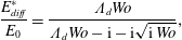 $$\begin{eqnarray}\frac{E_{diff}^{\ast }}{E_{0}}=\frac{\unicode[STIX]{x1D6EC}_{d}Wo}{\unicode[STIX]{x1D6EC}_{d}Wo-\text{i}-\text{i}\sqrt{\text{i}\,Wo}},\end{eqnarray}$$
where $\unicode[STIX]{x1D6EC}_{d}=(\unicode[STIX]{x2202}\unicode[STIX]{x1D6E4}/\unicode[STIX]{x2202}C_{s})/R_{0}$
is the dimensionless depletion depth (3.47). The monolayer behaves as if it were insoluble, so that
$\unicode[STIX]{x1D6EC}_{d}=(\unicode[STIX]{x2202}\unicode[STIX]{x1D6E4}/\unicode[STIX]{x2202}C_{s})/R_{0}$
is the dimensionless depletion depth (3.47). The monolayer behaves as if it were insoluble, so that $E_{diff}^{\ast }\rightarrow E_{0}$
when diffusive transport is so slow that surfactants desorbed during bubble compression do not diffuse away before they readsorb during bubble expansion (
$E_{diff}^{\ast }\rightarrow E_{0}$
when diffusive transport is so slow that surfactants desorbed during bubble compression do not diffuse away before they readsorb during bubble expansion ( $Wo\rightarrow \infty$
). By contrast,
$Wo\rightarrow \infty$
). By contrast, $\unicode[STIX]{x1D6E4}(t)$
remains nearly in equilibrium if the bubble oscillates much more slowly than required for diffusion (
$\unicode[STIX]{x1D6E4}(t)$
remains nearly in equilibrium if the bubble oscillates much more slowly than required for diffusion ( $Wo\rightarrow 0$
), in which limit the monolayer offers no resistance.
$Wo\rightarrow 0$
), in which limit the monolayer offers no resistance.
The real and imaginary parts of (4.52) correspond to the excess elastic and dissipative terms in (4.42). Separating these contributions and simplifying gives
 $$\begin{eqnarray}\frac{E_{diff}^{\ast }}{E_{0}}=\frac{1+\unicode[STIX]{x1D701}_{d}}{1+2\unicode[STIX]{x1D701}_{d}+2\unicode[STIX]{x1D701}_{d}^{2}(1+2\unicode[STIX]{x1D6EC}_{d}\unicode[STIX]{x1D701}_{d}+2\unicode[STIX]{x1D6EC}_{d}^{2}\unicode[STIX]{x1D701}_{d}^{2})}+\text{i}\frac{\unicode[STIX]{x1D701}_{d}(1+2\unicode[STIX]{x1D6EC}_{d}\unicode[STIX]{x1D701}_{d})}{1+2\unicode[STIX]{x1D701}_{d}+2\unicode[STIX]{x1D701}_{d}^{2}(1+2\unicode[STIX]{x1D6EC}_{d}\unicode[STIX]{x1D701}_{d}+2\unicode[STIX]{x1D6EC}_{d}\unicode[STIX]{x1D701}_{d}^{2})},\end{eqnarray}$$
where
 $$\begin{eqnarray}\unicode[STIX]{x1D701}_{d}=\frac{1}{L_{d}}\sqrt{\frac{D}{2\unicode[STIX]{x1D714}}}\end{eqnarray}$$
is the ratio of the diffusive oscillatory boundary layer thickness to the depletion depth (3.51),
 $$\begin{eqnarray}L_{d}=\frac{\unicode[STIX]{x2202}\unicode[STIX]{x1D6E4}}{\unicode[STIX]{x2202}C_{s}}.\end{eqnarray}$$
Bubbles with radii significantly larger than the depletion depth ( $\unicode[STIX]{x1D6EC}_{d}=L_{d}/R\ll 1$
) recover the classic results of Lucassen & van den Tempel (Reference Lucassen and van den Tempel1972) for oscillatory compression of planar interfaces, presented in § 4.2.1.
$\unicode[STIX]{x1D6EC}_{d}=L_{d}/R\ll 1$
) recover the classic results of Lucassen & van den Tempel (Reference Lucassen and van den Tempel1972) for oscillatory compression of planar interfaces, presented in § 4.2.1.
In the examples so far, the subphase was assumed to be infinitely deep so that the bulk fluid always contained enough surfactant to adsorb on to the interface given enough time. However, the bulk fluid may be entirely depleted of surfactant if the subphase is shallow, as may occur in thin films, coating flows, foams and concentrated emulsions. The film thickness $h$
then ‘cuts off’ the depletion depth
$h$
then ‘cuts off’ the depletion depth $L_{d}$
, and the film is said to be confined (Quéré Reference Quéré1999; Delacotte et al.
Reference Delacotte, Montel, Restagno, Scheid, Dollet, Stone, Langevin and Rio2012). Surface concentration perturbations are not diminished by adsorption/desorption if
$L_{d}$
, and the film is said to be confined (Quéré Reference Quéré1999; Delacotte et al.
Reference Delacotte, Montel, Restagno, Scheid, Dollet, Stone, Langevin and Rio2012). Surface concentration perturbations are not diminished by adsorption/desorption if $h\ll L_{d}$
, and the effective dilatational modulus is maximal (equal to the Marangoni modulus
$h\ll L_{d}$
, and the effective dilatational modulus is maximal (equal to the Marangoni modulus $E_{0}$
) for confined flows.
$E_{0}$
) for confined flows.
4.3 Damping of capillary waves
The calming effect of oil poured on the surface of water has been known among seafarers since the times of the ancient Greeks. Benjamin Franklin gave one of the earliest systematic accounts, claiming that a mere teaspoonful of oil was capable of rendering a half-acre pond ‘as smooth as a looking-glass’ (Franklin, Brownrigg & Farish Reference Franklin, Brownrigg and Farish1774). His own hypothesis was that the film of oil prevented wind from ‘catching’ the water, in turn preventing friction by gliding on the surface and damping wave formation. However, wave damping occurs far too quickly to result from a reduction in wind input alone.
Instead, surfactants dissipate wave energy and therefore play the dominant role in wave damping (Levich Reference Levich1962; Lucassen & Hansen Reference Lucassen and Hansen1966; Alpers & Hühnerfuss Reference Alpers and Hühnerfuss1989). In what follows, we will first outline wave motion on a clean interface, and later contrast it with waves on surfactant-laden interfaces. The surfaces of clean fluids are dilated or compressed at the nodes of surface waves, and surface rheology or Marangoni stresses resist such a deformation. Large surface elasticity or surface viscosity makes the interface act as effectively incompressible, suppressing the propagation of surface waves.
4.3.1 Waves on a clean liquid surface
The vertical displacement $\unicode[STIX]{x1D701}$
of a surface due to plane waves of wavelength
$\unicode[STIX]{x1D701}$
of a surface due to plane waves of wavelength $\unicode[STIX]{x1D706}$
propagating along the
$\unicode[STIX]{x1D706}$
propagating along the $x$
direction (figure 17) can be written
$x$
direction (figure 17) can be written
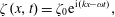 $$\begin{eqnarray}\unicode[STIX]{x1D701}(x,t)=\unicode[STIX]{x1D701}_{0}\text{e}^{\text{i}(kx-\unicode[STIX]{x1D714}t)},\end{eqnarray}$$
where $k=2\unicode[STIX]{x03C0}/\unicode[STIX]{x1D706}$
and
$k=2\unicode[STIX]{x03C0}/\unicode[STIX]{x1D706}$
and $\unicode[STIX]{x1D714}$
are, respectively, the wavenumber and frequency. For small wave amplitudes, the nonlinear term in the Navier–Stokes equation is negligible (Levich Reference Levich1962; Probstein Reference Probstein1994) and the hydrodynamic governing equations are the unsteady Stokes equations.
$\unicode[STIX]{x1D714}$
are, respectively, the wavenumber and frequency. For small wave amplitudes, the nonlinear term in the Navier–Stokes equation is negligible (Levich Reference Levich1962; Probstein Reference Probstein1994) and the hydrodynamic governing equations are the unsteady Stokes equations.
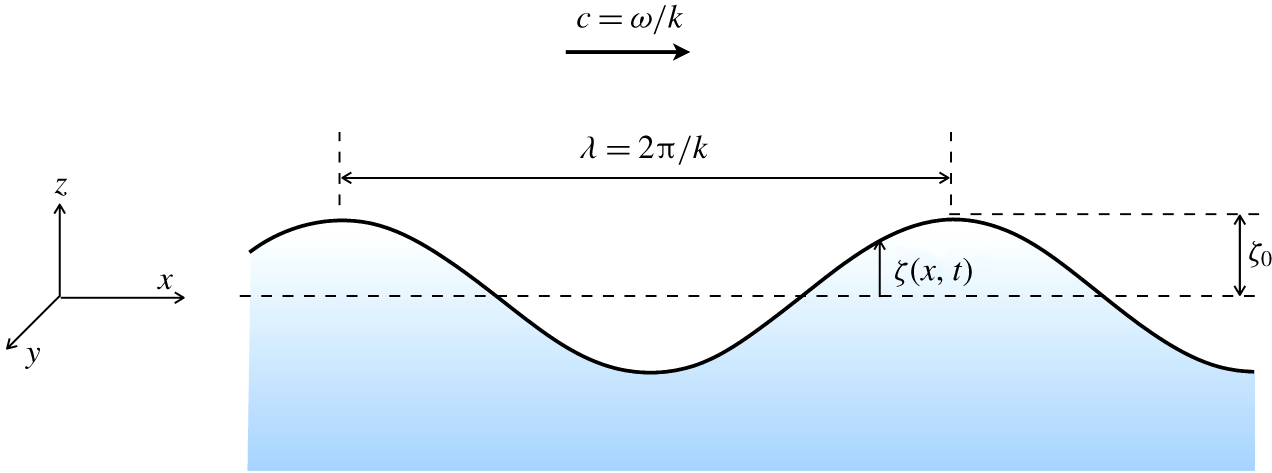
Figure 17. A planar wave of amplitude $\unicode[STIX]{x1D701}_{0}$
, length
$\unicode[STIX]{x1D701}_{0}$
, length $\unicode[STIX]{x1D706}$
and frequency
$\unicode[STIX]{x1D706}$
and frequency $\unicode[STIX]{x1D714}$
.
$\unicode[STIX]{x1D714}$
.
Waves are driven by the balance between fluid inertia and the restoring forces of gravity and/or surface tension. The excess hydrostatic pressure due to the disturbance is
 $$\begin{eqnarray}p_{g}=\unicode[STIX]{x1D70C}g\unicode[STIX]{x1D701},\end{eqnarray}$$
and the excess capillary pressure, following the Young–Laplace equation and assuming small curvatures, is
 $$\begin{eqnarray}p_{c}=-\unicode[STIX]{x1D6FE}\frac{\unicode[STIX]{x2202}^{2}\unicode[STIX]{x1D701}}{\unicode[STIX]{x2202}x^{2}}=\unicode[STIX]{x1D6FE}k^{2}\unicode[STIX]{x1D701}.\end{eqnarray}$$
The ratio of hydrostatic and capillary pressures is the Bond number,
 $$\begin{eqnarray}Bo=\frac{p_{g}}{p_{c}}=\frac{\unicode[STIX]{x1D70C}g}{\unicode[STIX]{x1D6FE}k^{2}}.\end{eqnarray}$$
Short wavelengths ( $Bo\ll 1$
) correspond to capillary waves (
$Bo\ll 1$
) correspond to capillary waves ( $\unicode[STIX]{x1D706}\lesssim O(1~\text{cm})$
for water), whereas large wavelengths (
$\unicode[STIX]{x1D706}\lesssim O(1~\text{cm})$
for water), whereas large wavelengths ( $Bo\gg 1$
) correspond to gravity waves.
$Bo\gg 1$
) correspond to gravity waves.
Inviscid flows are simplest, as they are irrotational in this configuration, and can therefore be described by a velocity potential
 $$\begin{eqnarray}\boldsymbol{v}=\unicode[STIX]{x1D735}\unicode[STIX]{x1D719},\quad \text{and}\quad \unicode[STIX]{x1D6FB}^{2}\unicode[STIX]{x1D719}=0.\end{eqnarray}$$
Linearity and continuity require
 $$\begin{eqnarray}\unicode[STIX]{x1D719}(x,z,t)=A\text{e}^{kz}\text{e}^{\text{i}(kx-\unicode[STIX]{x1D714}t)},\end{eqnarray}$$
so that the linearized inviscid Navier–Stokes equation gives
 $$\begin{eqnarray}\left.\frac{\unicode[STIX]{x2202}\unicode[STIX]{x1D719}}{\unicode[STIX]{x2202}t}\right|_{z=0}=-\left(g+\frac{\unicode[STIX]{x1D6FE}k^{2}}{\unicode[STIX]{x1D70C}}\right)\unicode[STIX]{x1D701},\end{eqnarray}$$
approximating the interface to be at $z=0$
, with
$z=0$
, with $O(\unicode[STIX]{x1D701}^{2})$
corrections. Imposing the kinematic condition
$O(\unicode[STIX]{x1D701}^{2})$
corrections. Imposing the kinematic condition $D\unicode[STIX]{x1D701}/Dt=v_{z}$
at the interface then gives
$D\unicode[STIX]{x1D701}/Dt=v_{z}$
at the interface then gives
 $$\begin{eqnarray}\unicode[STIX]{x1D714}_{0}=\left(gk+\frac{\unicode[STIX]{x1D6FE}k^{3}}{\unicode[STIX]{x1D70C}}\right)^{1/2}=\sqrt{\frac{\unicode[STIX]{x1D6FE}k^{3}}{\unicode[STIX]{x1D70C}}}(1+Bo)^{1/2},\end{eqnarray}$$
where $Bo$
is the Bond number (4.59). From the dispersion relation (4.63), the wave velocity is given by
$Bo$
is the Bond number (4.59). From the dispersion relation (4.63), the wave velocity is given by
 $$\begin{eqnarray}c=\frac{\unicode[STIX]{x1D714}_{0}}{k},\end{eqnarray}$$
with a minimum $c_{min}\approx 20~\text{cm}~\text{s}^{-1}$
for water.
$c_{min}\approx 20~\text{cm}~\text{s}^{-1}$
for water.
Waves described by (4.63) neither grow nor decay when the fluid is inviscid and the interface is clean. However, waves decay in fluids with finite viscosity. The relative strength of wave damping is captured by the ratio of viscous stresses to inertial stresses,
 $$\begin{eqnarray}m=\frac{\unicode[STIX]{x1D708}k^{2}}{\unicode[STIX]{x1D714}_{0}}=\frac{2\unicode[STIX]{x03C0}\unicode[STIX]{x1D708}}{c\unicode[STIX]{x1D706}},\end{eqnarray}$$
where $\unicode[STIX]{x1D708}=\unicode[STIX]{x1D702}/\unicode[STIX]{x1D70C}$
is the kinematic viscosity. Based on the minimum phase velocity in water,
$\unicode[STIX]{x1D708}=\unicode[STIX]{x1D702}/\unicode[STIX]{x1D70C}$
is the kinematic viscosity. Based on the minimum phase velocity in water, $m<1$
for wavelengths larger than
$m<1$
for wavelengths larger than $\unicode[STIX]{x1D706}\gtrsim 0.1~\text{mm}$
(Levich Reference Levich1962). Viscous stresses are therefore typically weak relative to inertia, and it is safe to assume that the wave frequency departs only slightly from its inviscid value
$\unicode[STIX]{x1D706}\gtrsim 0.1~\text{mm}$
(Levich Reference Levich1962). Viscous stresses are therefore typically weak relative to inertia, and it is safe to assume that the wave frequency departs only slightly from its inviscid value $\unicode[STIX]{x1D714}_{0}$
, so that
$\unicode[STIX]{x1D714}_{0}$
, so that
 $$\begin{eqnarray}\unicode[STIX]{x1D701}(x,t)=\unicode[STIX]{x1D701}_{0}\text{e}^{\text{i}(kx-\unicode[STIX]{x1D714}_{0}t)+\unicode[STIX]{x1D6FD}t},\end{eqnarray}$$
where $|\unicode[STIX]{x1D6FD}|\ll \unicode[STIX]{x1D714}_{0}$
gives a weak viscous damping. The negative real part of
$|\unicode[STIX]{x1D6FD}|\ll \unicode[STIX]{x1D714}_{0}$
gives a weak viscous damping. The negative real part of $\unicode[STIX]{x1D6FD}$
is the decay rate, and its imaginary part gives a small correction to the wave frequency due to fluid viscosity.
$\unicode[STIX]{x1D6FD}$
is the decay rate, and its imaginary part gives a small correction to the wave frequency due to fluid viscosity.
The non-irrotational nature of viscous flows necessitates a streamfunction $\unicode[STIX]{x1D713}$
in addition to the potential function
$\unicode[STIX]{x1D713}$
in addition to the potential function $\unicode[STIX]{x1D719}$
. Solving for the velocity, pressure and
$\unicode[STIX]{x1D719}$
. Solving for the velocity, pressure and $\unicode[STIX]{x1D6FD}$
based on
$\unicode[STIX]{x1D6FD}$
based on $\unicode[STIX]{x1D719}$
and
$\unicode[STIX]{x1D719}$
and $\unicode[STIX]{x1D713}$
is tedious – see Levich (Reference Levich1962) for details – here we simply present the resultant damping rate,
$\unicode[STIX]{x1D713}$
is tedious – see Levich (Reference Levich1962) for details – here we simply present the resultant damping rate,
 $$\begin{eqnarray}\unicode[STIX]{x1D6FD}_{clean}=\text{Re}[\unicode[STIX]{x1D6FD}]=-2m\unicode[STIX]{x1D714}_{0}=-2\unicode[STIX]{x1D708}k^{2}.\end{eqnarray}$$
The damping time scale $\unicode[STIX]{x1D6FD}_{clean}^{-1}$
can be interpreted as the time taken for vorticity generated by shear stresses to diffuse a depth comparable to the wavelength
$\unicode[STIX]{x1D6FD}_{clean}^{-1}$
can be interpreted as the time taken for vorticity generated by shear stresses to diffuse a depth comparable to the wavelength $\unicode[STIX]{x1D706}$
.
$\unicode[STIX]{x1D706}$
.
In what follows, we examine how surfactants modify the damping rate $\unicode[STIX]{x1D6FD}$
. Levich (Reference Levich1962) shows the effect of surfactants to be significant only when
$\unicode[STIX]{x1D6FD}$
. Levich (Reference Levich1962) shows the effect of surfactants to be significant only when $\unicode[STIX]{x1D706}\lesssim 10~\text{cm}$
, and therefore affect capillary waves more prominently than gravity waves. We will therefore restrict our attention to capillary waves (
$\unicode[STIX]{x1D706}\lesssim 10~\text{cm}$
, and therefore affect capillary waves more prominently than gravity waves. We will therefore restrict our attention to capillary waves ( $Bo\ll 1$
) in the following sections, and approximate
$Bo\ll 1$
) in the following sections, and approximate $\unicode[STIX]{x1D714}_{0}\approx \sqrt{\unicode[STIX]{x1D6FE}k^{3}/\unicode[STIX]{x1D70C}}$
. As Franklin et al. (Reference Franklin, Brownrigg and Farish1774) noted over two centuries ago, large waves on a stormy sea are unaffected, whereas smaller ripples are smoothed out resulting in ‘glassy’ surfaces.
$\unicode[STIX]{x1D714}_{0}\approx \sqrt{\unicode[STIX]{x1D6FE}k^{3}/\unicode[STIX]{x1D70C}}$
. As Franklin et al. (Reference Franklin, Brownrigg and Farish1774) noted over two centuries ago, large waves on a stormy sea are unaffected, whereas smaller ripples are smoothed out resulting in ‘glassy’ surfaces.
4.3.2 Marangoni damping due to insoluble and surface inviscid surfactants
Surfactants strengthen wave damping through two main mechanisms – Marangoni stresses and surface rheology – and we start with the former. The simplest case is a surface-inviscid monolayer, for which $\unicode[STIX]{x1D702}_{s}=\unicode[STIX]{x1D705}_{s}=0$
. Additionally, surface concentration gradients do not relax by adsorption/desorption in insoluble monolayers, in which case
$\unicode[STIX]{x1D702}_{s}=\unicode[STIX]{x1D705}_{s}=0$
. Additionally, surface concentration gradients do not relax by adsorption/desorption in insoluble monolayers, in which case $E$
is equal to the Marangoni modulus
$E$
is equal to the Marangoni modulus $E_{0}$
(§ 2.4.2). Surface diffusion may also weaken the Marangoni effect by smoothing out gradients in
$E_{0}$
(§ 2.4.2). Surface diffusion may also weaken the Marangoni effect by smoothing out gradients in $\unicode[STIX]{x1D6E4}$
, but we will neglect diffusion by assuming the time to diffuse the wavelength
$\unicode[STIX]{x1D6E4}$
, but we will neglect diffusion by assuming the time to diffuse the wavelength $\unicode[STIX]{x1D706}^{2}/D_{s}$
is much longer than the oscillation period
$\unicode[STIX]{x1D706}^{2}/D_{s}$
is much longer than the oscillation period $\unicode[STIX]{x1D714}_{0}$
.
$\unicode[STIX]{x1D714}_{0}$
.
The surface concentration is perturbed away from its equilibrium value $\unicode[STIX]{x1D6E4}_{0}$
via
$\unicode[STIX]{x1D6E4}_{0}$
via
 $$\begin{eqnarray}\unicode[STIX]{x1D6E4}(x,t)=\unicode[STIX]{x1D6E4}_{0}+\unicode[STIX]{x1D6FF}\unicode[STIX]{x1D6E4}\text{e}^{\text{i}(kx-\unicode[STIX]{x1D714}_{0}t)+\unicode[STIX]{x1D6FD}t},\end{eqnarray}$$
where $\unicode[STIX]{x1D6FF}\unicode[STIX]{x1D6E4}\ll \unicode[STIX]{x1D6E4}_{0}$
. As with the vertical displacement
$\unicode[STIX]{x1D6FF}\unicode[STIX]{x1D6E4}\ll \unicode[STIX]{x1D6E4}_{0}$
. As with the vertical displacement $\unicode[STIX]{x1D701}(x,t)$
(4.66), we assume that subphase viscous effects are weak, so that the frequency is well approximated by its inviscid value
$\unicode[STIX]{x1D701}(x,t)$
(4.66), we assume that subphase viscous effects are weak, so that the frequency is well approximated by its inviscid value $\unicode[STIX]{x1D714}_{0}$
, and that the damping rate
$\unicode[STIX]{x1D714}_{0}$
, and that the damping rate $|\unicode[STIX]{x1D6FD}|\ll \unicode[STIX]{x1D714}_{0}$
. For small surface velocities, the surfactant conservation equation (3.10) gives
$|\unicode[STIX]{x1D6FD}|\ll \unicode[STIX]{x1D714}_{0}$
. For small surface velocities, the surfactant conservation equation (3.10) gives
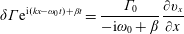 $$\begin{eqnarray}\unicode[STIX]{x1D6FF}\unicode[STIX]{x1D6E4}\text{e}^{\text{i}(kx-\unicode[STIX]{x1D714}_{0}t)+\unicode[STIX]{x1D6FD}t}=\frac{\unicode[STIX]{x1D6E4}_{0}}{-\text{i}\unicode[STIX]{x1D714}_{0}+\unicode[STIX]{x1D6FD}}\frac{\unicode[STIX]{x2202}v_{x}}{\unicode[STIX]{x2202}x}\end{eqnarray}$$
to leading order, so that the normal and tangential stress boundary conditions (3.8) for a surface-inviscid monolayer are
 $$\begin{eqnarray}\displaystyle & \displaystyle -p+2\unicode[STIX]{x1D702}\frac{\unicode[STIX]{x2202}v_{z}}{\unicode[STIX]{x2202}z}=\unicode[STIX]{x1D6FE}(\unicode[STIX]{x1D6E4}_{0})\frac{\unicode[STIX]{x2202}^{2}\unicode[STIX]{x1D701}}{\unicode[STIX]{x2202}x^{2}}, & \displaystyle\end{eqnarray}$$
 $$\begin{eqnarray}\displaystyle & \displaystyle \unicode[STIX]{x1D702}\left(\frac{\unicode[STIX]{x2202}v_{x}}{\unicode[STIX]{x2202}z}+\frac{\unicode[STIX]{x2202}v_{z}}{\unicode[STIX]{x2202}x}\right)=-\frac{E_{0}}{\unicode[STIX]{x1D6E4}_{0}}\frac{\unicode[STIX]{x2202}\unicode[STIX]{x1D6E4}}{\unicode[STIX]{x2202}x}=\frac{E_{0}}{\text{i}\unicode[STIX]{x1D714}_{0}-\unicode[STIX]{x1D6FD}}\frac{\unicode[STIX]{x2202}^{2}v_{x}}{\unicode[STIX]{x2202}x^{2}}. & \displaystyle\end{eqnarray}$$ $\unicode[STIX]{x1D6FD}$
to depend on the relative magnitudes of
$\unicode[STIX]{x1D6FD}$
to depend on the relative magnitudes of $\unicode[STIX]{x1D6FE}(\unicode[STIX]{x1D6E4}_{0})$
and
$\unicode[STIX]{x1D6FE}(\unicode[STIX]{x1D6E4}_{0})$
and $E_{0}(\unicode[STIX]{x1D6E4}_{0})$
.
$E_{0}(\unicode[STIX]{x1D6E4}_{0})$
.
Solving the unsteady Stokes equations with boundary conditions (4.70) gives the fluid velocity and the damping rate $\unicode[STIX]{x1D6FD}$
. The calculation is tedious, but analytically tractable, in the limits of weak viscosity (
$\unicode[STIX]{x1D6FD}$
. The calculation is tedious, but analytically tractable, in the limits of weak viscosity ( $m=\unicode[STIX]{x1D708}k^{2}/\unicode[STIX]{x1D714}_{0}\ll 1$
) and small damping rate (
$m=\unicode[STIX]{x1D708}k^{2}/\unicode[STIX]{x1D714}_{0}\ll 1$
) and small damping rate ( $|\unicode[STIX]{x1D6FD}|\ll \unicode[STIX]{x1D714}_{0}$
), giving (Levich Reference Levich1962; Alpers & Hühnerfuss Reference Alpers and Hühnerfuss1989)
$|\unicode[STIX]{x1D6FD}|\ll \unicode[STIX]{x1D714}_{0}$
), giving (Levich Reference Levich1962; Alpers & Hühnerfuss Reference Alpers and Hühnerfuss1989)
 $$\begin{eqnarray}\frac{\text{Re}[\unicode[STIX]{x1D6FD}]}{\unicode[STIX]{x1D714}_{0}}\approx -\frac{1}{2\sqrt{2}}\frac{Ma_{\unicode[STIX]{x1D6FE}}^{2}\sqrt{m}-4Ma_{\unicode[STIX]{x1D6FE}}m^{3/2}+4\sqrt{2}m^{2}}{Ma_{\unicode[STIX]{x1D6FE}}^{2}+m-Ma_{\unicode[STIX]{x1D6FE}}\sqrt{2m}}.\end{eqnarray}$$
Here, the modified Marangoni number $Ma_{\unicode[STIX]{x1D6FE}}$
(table 3) quantifies the competition between interfacial area creation due to capillary forces and resistance to interfacial stretching due to Marangoni forces
$Ma_{\unicode[STIX]{x1D6FE}}$
(table 3) quantifies the competition between interfacial area creation due to capillary forces and resistance to interfacial stretching due to Marangoni forces
 $$\begin{eqnarray}Ma_{\unicode[STIX]{x1D6FE}}=\frac{E_{0}(\unicode[STIX]{x1D6E4}_{0})}{\unicode[STIX]{x1D6FE}(\unicode[STIX]{x1D6E4}_{0})}=\frac{E_{0}}{\unicode[STIX]{x1D702}c}\times \frac{\unicode[STIX]{x1D702}c}{\unicode[STIX]{x1D6FE}}=Ma\times Ca.\end{eqnarray}$$
Reverse Marangoni flows immobilize the interface when $Ma_{\unicode[STIX]{x1D6FE}}\gg 1$
or
$Ma_{\unicode[STIX]{x1D6FE}}\gg 1$
or $E_{0}\gg \unicode[STIX]{x1D6FE}$
, in which case the interface behaves like an incompressible sheet with
$E_{0}\gg \unicode[STIX]{x1D6FE}$
, in which case the interface behaves like an incompressible sheet with
 $$\begin{eqnarray}\unicode[STIX]{x1D6FD}_{stiff}=\text{Re}[\unicode[STIX]{x1D6FD}(Ma_{\unicode[STIX]{x1D6FE}}\rightarrow \infty )]=-\frac{1}{2\sqrt{2}}\unicode[STIX]{x1D714}_{0}\sqrt{m}=-\frac{1}{2\sqrt{2}}\sqrt{\unicode[STIX]{x1D714}_{0}\unicode[STIX]{x1D708}k^{2}}.\end{eqnarray}$$
By contrast, weak $E_{0}$
gives
$E_{0}$
gives $Ma_{\unicode[STIX]{x1D6FE}}\ll 1$
and recovers the clean interface limit
$Ma_{\unicode[STIX]{x1D6FE}}\ll 1$
and recovers the clean interface limit $\unicode[STIX]{x1D6FD}_{clean}$
(4.67). The ratio of the damping coefficient in the two limits is
$\unicode[STIX]{x1D6FD}_{clean}$
(4.67). The ratio of the damping coefficient in the two limits is
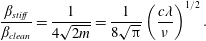 $$\begin{eqnarray}\frac{\unicode[STIX]{x1D6FD}_{stiff}}{\unicode[STIX]{x1D6FD}_{clean}}=\frac{1}{4\sqrt{2m}}=\frac{1}{8\sqrt{\unicode[STIX]{x03C0}}}\left(\frac{c\unicode[STIX]{x1D706}}{\unicode[STIX]{x1D708}}\right)^{1/2}.\end{eqnarray}$$
Because wave speeds are greater than $c_{min}\approx 0.2~\text{m}~\text{s}^{-1}$
on water–air interfaces,
$c_{min}\approx 0.2~\text{m}~\text{s}^{-1}$
on water–air interfaces, $\unicode[STIX]{x1D6FD}_{stiff}>\unicode[STIX]{x1D6FD}_{clean}$
for waves with millimetre (or larger) wavelength. Typical capillary waves therefore decay more rapidly when surfactants are present.
$\unicode[STIX]{x1D6FD}_{stiff}>\unicode[STIX]{x1D6FD}_{clean}$
for waves with millimetre (or larger) wavelength. Typical capillary waves therefore decay more rapidly when surfactants are present.
Notably, the damping coefficient depends non-monotonically on $Ma_{\unicode[STIX]{x1D6FE}}$
(figure 18), with a maximum value
$Ma_{\unicode[STIX]{x1D6FE}}$
(figure 18), with a maximum value $\unicode[STIX]{x1D6FD}_{max}\approx 2\unicode[STIX]{x1D6FD}_{stiff}$
that occurs at an intermediate Marangoni number, as reported in both experiments and simulations (Davies & Vose Reference Davies and Vose1965; Alpers & Hühnerfuss Reference Alpers and Hühnerfuss1989). Lucassen (Reference Lucassen1968) ascribes this maximum to a resonance-like mechanism between transverse capillary waves and longitudinal Marangoni waves. Damping is maximum when the wavelengths of these transverse and longitudinal waves are equal.
$\unicode[STIX]{x1D6FD}_{max}\approx 2\unicode[STIX]{x1D6FD}_{stiff}$
that occurs at an intermediate Marangoni number, as reported in both experiments and simulations (Davies & Vose Reference Davies and Vose1965; Alpers & Hühnerfuss Reference Alpers and Hühnerfuss1989). Lucassen (Reference Lucassen1968) ascribes this maximum to a resonance-like mechanism between transverse capillary waves and longitudinal Marangoni waves. Damping is maximum when the wavelengths of these transverse and longitudinal waves are equal.
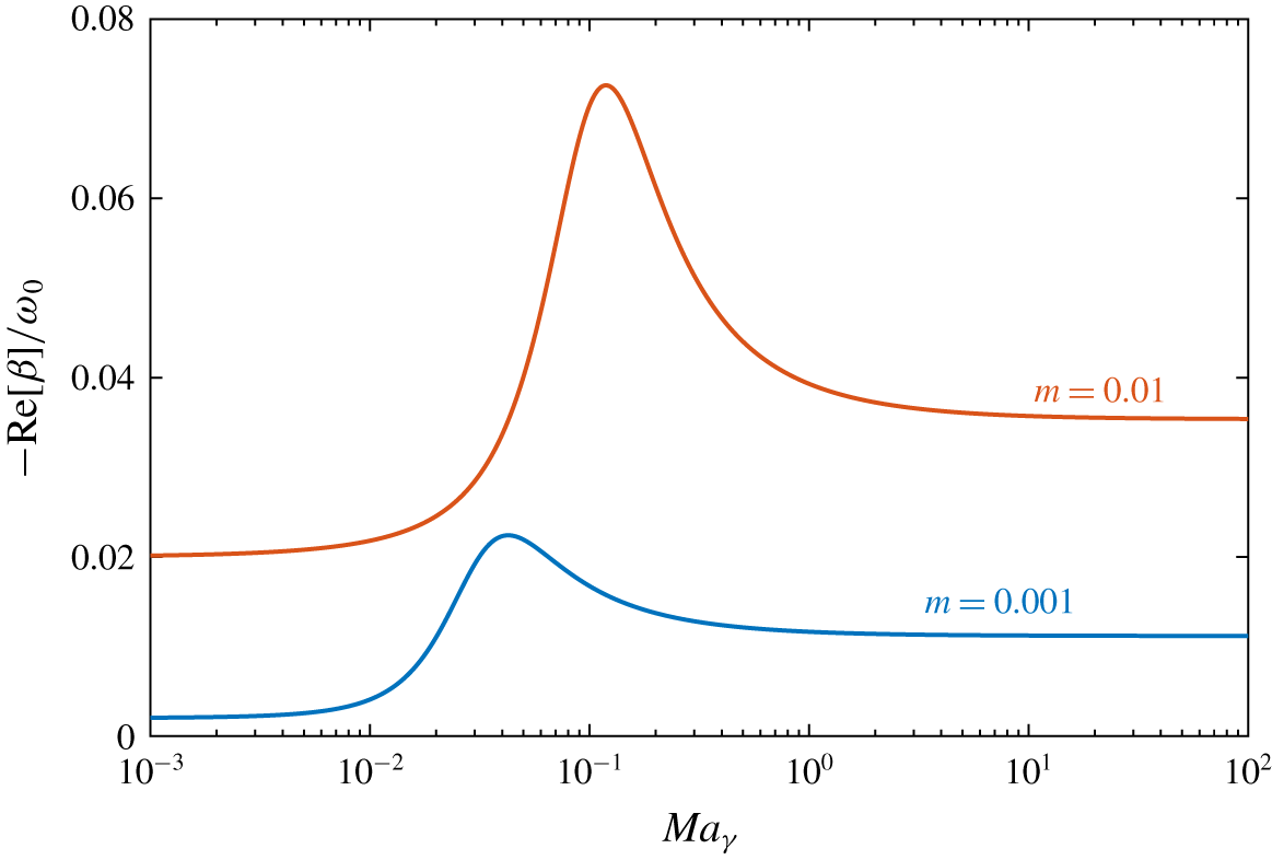
Figure 18. Capillary wave damping rate $\unicode[STIX]{x1D6FD}$
(4.71) as a function of the Marangoni number
$\unicode[STIX]{x1D6FD}$
(4.71) as a function of the Marangoni number $Ma_{\unicode[STIX]{x1D6FE}}=E_{0}/\unicode[STIX]{x1D6FE}$
and the normalized fluid viscosity
$Ma_{\unicode[STIX]{x1D6FE}}=E_{0}/\unicode[STIX]{x1D6FE}$
and the normalized fluid viscosity $m=\unicode[STIX]{x1D708}k^{2}/\unicode[STIX]{x1D714}_{0}$
. The damping rate asymptotes to
$m=\unicode[STIX]{x1D708}k^{2}/\unicode[STIX]{x1D714}_{0}$
. The damping rate asymptotes to $\unicode[STIX]{x1D6FD}_{clean}=-2m\unicode[STIX]{x1D714}_{0}$
when Marangoni flows are weak (
$\unicode[STIX]{x1D6FD}_{clean}=-2m\unicode[STIX]{x1D714}_{0}$
when Marangoni flows are weak ( $Ma_{\unicode[STIX]{x1D6FE}}\ll 1$
) and to
$Ma_{\unicode[STIX]{x1D6FE}}\ll 1$
) and to $\unicode[STIX]{x1D6FD}_{stiff}=-(\unicode[STIX]{x1D714}_{0}/2)\sqrt{m/2}$
when the interface is immobilized (
$\unicode[STIX]{x1D6FD}_{stiff}=-(\unicode[STIX]{x1D714}_{0}/2)\sqrt{m/2}$
when the interface is immobilized ( $Ma_{\unicode[STIX]{x1D6FE}}\gg 1$
). Waves decay faster in a more viscous fluid (larger
$Ma_{\unicode[STIX]{x1D6FE}}\gg 1$
). Waves decay faster in a more viscous fluid (larger $m$
) for all
$m$
) for all $Ma_{\unicode[STIX]{x1D6FE}}$
.
$Ma_{\unicode[STIX]{x1D6FE}}$
.
Probstein (Reference Probstein1994) notes that $\unicode[STIX]{x1D6FD}_{stiff}$
can be estimated by treating the interface as an incompressible plate. The damping coefficient in general takes the form
$\unicode[STIX]{x1D6FD}_{stiff}$
can be estimated by treating the interface as an incompressible plate. The damping coefficient in general takes the form $\unicode[STIX]{x1D6FD}\sim -\unicode[STIX]{x1D708}k/d$
, where
$\unicode[STIX]{x1D6FD}\sim -\unicode[STIX]{x1D708}k/d$
, where $d$
is viscous gradient length scale in the bulk. Without surfactants, the dissipation extends to a depth
$d$
is viscous gradient length scale in the bulk. Without surfactants, the dissipation extends to a depth $d\sim k^{-1}$
, and
$d\sim k^{-1}$
, and $\unicode[STIX]{x1D6FD}=\unicode[STIX]{x1D6FD}_{clean}\sim -\unicode[STIX]{x1D708}k^{2}$
in agreement with (4.67). When surfactants immobilize the surface via Marangoni flows, the viscous boundary layer under the surface is akin to that of an incompressible plate oscillating at frequency
$\unicode[STIX]{x1D6FD}=\unicode[STIX]{x1D6FD}_{clean}\sim -\unicode[STIX]{x1D708}k^{2}$
in agreement with (4.67). When surfactants immobilize the surface via Marangoni flows, the viscous boundary layer under the surface is akin to that of an incompressible plate oscillating at frequency $\unicode[STIX]{x1D714}$
. This is Stokes’ second problem, revealing a viscous boundary layer that extends to a depth
$\unicode[STIX]{x1D714}$
. This is Stokes’ second problem, revealing a viscous boundary layer that extends to a depth $d\sim (\unicode[STIX]{x1D708}/\unicode[STIX]{x1D714})^{1/2}$
, with damping rate
$d\sim (\unicode[STIX]{x1D708}/\unicode[STIX]{x1D714})^{1/2}$
, with damping rate $\unicode[STIX]{x1D6FD}_{stiff}\sim -(\unicode[STIX]{x1D708}\unicode[STIX]{x1D714})^{1/2}k$
.
$\unicode[STIX]{x1D6FD}_{stiff}\sim -(\unicode[STIX]{x1D708}\unicode[STIX]{x1D714})^{1/2}k$
.
The enhanced damping mechanism is illustrated in figure 19. Fluid elements on and near a surfactant-free interface travel in circular trajectories. Surfactants drive Marangoni flows that act to immobilize the interface, distorting these circular trajectories. The change from near-vertical motion at the interface to circular trajectories in the subphase increases velocity gradients and viscous dissipation. Notably, damping still occurs due to bulk viscous dissipation: surface incompressibility due to reverse Marangoni flow modifies the bulk velocity field in a manner that amplifies viscous dissipation in the bulk (§ 3.3.2).

Figure 19. (a) Circular motion of interfacial fluid particles on the clean surface of a wave moving to the right. The solid blue arrows along the interface depict compression and expansion of the surface. (b) Surfactants distort circular trajectories via Marangoni flows (red dashed arrows) that oppose the compression and expansion of the interface. The trajectories of fluid elements are then distorted, becoming straight lines in the $Ma_{\unicode[STIX]{x1D6FE}}\rightarrow \infty$
limit.
$Ma_{\unicode[STIX]{x1D6FE}}\rightarrow \infty$
limit.
4.3.3 Damping due to soluble and/or surface viscous surfactants
The surface flow generated by the motion of a wave creates alternating regions of dilatation and compression (figure 19). Any putative surface-viscous stresses would resist such a deformation. Note also that surface shear and surface dilatational viscosities appear inseparably in the Boussinesq–Scriven equation (3.118) for 1-D deformations, as occurs in plane waves. In other words, a monolayer with finite surface shear viscosity $\unicode[STIX]{x1D702}_{s}$
resists one-dimensional stretching and compression, even if the surface dilatational viscosity
$\unicode[STIX]{x1D702}_{s}$
resists one-dimensional stretching and compression, even if the surface dilatational viscosity $\unicode[STIX]{x1D705}_{s}$
is negligible.
$\unicode[STIX]{x1D705}_{s}$
is negligible.
Recall from the oscillatory dynamics of surfactant-covered bubbles (§ 4.2.2) that additional viscous stresses arise due to excess surface rheology as well as adsorption/desorption. The tangential stress balance (3.94) for a Newtonian monolayer undergoing 1-D deformation is
 $$\begin{eqnarray}\unicode[STIX]{x1D702}\left(\frac{\unicode[STIX]{x2202}v_{x}}{\unicode[STIX]{x2202}z}+\frac{\unicode[STIX]{x2202}v_{z}}{\unicode[STIX]{x2202}x}\right)=-\frac{E_{0}}{\unicode[STIX]{x1D6E4}_{0}}\frac{\unicode[STIX]{x2202}\unicode[STIX]{x1D6E4}}{\unicode[STIX]{x2202}x}+(\unicode[STIX]{x1D702}_{s}+\unicode[STIX]{x1D705}_{s})\frac{\unicode[STIX]{x2202}^{2}v_{x}}{\unicode[STIX]{x2202}x^{2}},\end{eqnarray}$$
where changes in $\unicode[STIX]{x1D6E4}$
now drive adsorption/desorption fluxes. In what follows, we will assume diffusion-limited adsorption (§ 3.2); kinetically limited systems follow similar trends. Solving the bulk diffusion equation and substituting in (4.75) while assuming small perturbations as in (4.68) gives
$\unicode[STIX]{x1D6E4}$
now drive adsorption/desorption fluxes. In what follows, we will assume diffusion-limited adsorption (§ 3.2); kinetically limited systems follow similar trends. Solving the bulk diffusion equation and substituting in (4.75) while assuming small perturbations as in (4.68) gives
 $$\begin{eqnarray}\unicode[STIX]{x1D702}\left(\frac{\unicode[STIX]{x2202}v_{x}}{\unicode[STIX]{x2202}z}+\frac{\unicode[STIX]{x2202}v_{z}}{\unicode[STIX]{x2202}x}\right)=\frac{E_{eff}}{\text{i}\unicode[STIX]{x1D714}_{0}-\unicode[STIX]{x1D6FD}}\frac{\unicode[STIX]{x2202}^{2}v_{x}}{\unicode[STIX]{x2202}x^{2}},\end{eqnarray}$$
which is similar to the insoluble tangential stress balance (4.70b ) except with a complex effective modulus
 $$\begin{eqnarray}E_{eff}=E^{\ast }+(\text{i}\unicode[STIX]{x1D714}_{0}-\unicode[STIX]{x1D6FD})(\unicode[STIX]{x1D702}_{s}+\unicode[STIX]{x1D705}_{s}),\end{eqnarray}$$
where $E^{\ast }(\unicode[STIX]{x1D714})$
is the complex modulus for uniform oscillatory deformation (4.34).
$E^{\ast }(\unicode[STIX]{x1D714})$
is the complex modulus for uniform oscillatory deformation (4.34).
The real part of the effective dilatational modulus $E_{eff}$
(4.77) quantifies the strength of reverse Marangoni flows. Rapid adsorption eliminates Marangoni forces, giving
$E_{eff}$
(4.77) quantifies the strength of reverse Marangoni flows. Rapid adsorption eliminates Marangoni forces, giving $\text{Re}[E_{eff}]\approx 0$
(assuming
$\text{Re}[E_{eff}]\approx 0$
(assuming $|\unicode[STIX]{x1D6FD}|\ll \unicode[STIX]{x1D714}_{0}$
). By contrast, reverse Marangoni flows are strongest for negligibly slow adsorption, whereupon
$|\unicode[STIX]{x1D6FD}|\ll \unicode[STIX]{x1D714}_{0}$
). By contrast, reverse Marangoni flows are strongest for negligibly slow adsorption, whereupon $\text{Re}[E_{eff}]\approx E_{0}$
(4.34). Solubility effectively reduces the dynamic Gibbs modulus
$\text{Re}[E_{eff}]\approx E_{0}$
(4.34). Solubility effectively reduces the dynamic Gibbs modulus $E=\text{Re}[E^{\ast }]$
(figure 16) and therefore decreases the damping rate
$E=\text{Re}[E^{\ast }]$
(figure 16) and therefore decreases the damping rate $\unicode[STIX]{x1D6FD}(E)$
. Indeed, Franklin et al. (Reference Franklin, Brownrigg and Farish1774) and Levich (Reference Levich1962) note that sailors report that waves are damped more with animal and vegetable oils (with insoluble fatty acids) than with soluble mineral oils. The imaginary part of
$\unicode[STIX]{x1D6FD}(E)$
. Indeed, Franklin et al. (Reference Franklin, Brownrigg and Farish1774) and Levich (Reference Levich1962) note that sailors report that waves are damped more with animal and vegetable oils (with insoluble fatty acids) than with soluble mineral oils. The imaginary part of $E_{eff}$
(4.77) quantifies surface-viscous resistance to wave motion. In addition to
$E_{eff}$
(4.77) quantifies surface-viscous resistance to wave motion. In addition to $\unicode[STIX]{x1D702}_{s}$
and
$\unicode[STIX]{x1D702}_{s}$
and $\unicode[STIX]{x1D705}_{s}$
,
$\unicode[STIX]{x1D705}_{s}$
, $\text{Im}[E_{eff}]$
contains a contribution
$\text{Im}[E_{eff}]$
contains a contribution $\unicode[STIX]{x1D705}_{s}^{ads}=\text{Im}[E^{\ast }]$
(4.34), which becomes significant when
$\unicode[STIX]{x1D705}_{s}^{ads}=\text{Im}[E^{\ast }]$
(4.34), which becomes significant when $\unicode[STIX]{x1D714}_{0}$
is comparable to the sorption time.
$\unicode[STIX]{x1D714}_{0}$
is comparable to the sorption time.
The full calculation of $\unicode[STIX]{x1D6FD}$
is complicated, and we do not pursue it here. However, the similarity between (4.76) and (4.70b
) suggests that the damping rate
$\unicode[STIX]{x1D6FD}$
is complicated, and we do not pursue it here. However, the similarity between (4.76) and (4.70b
) suggests that the damping rate $\unicode[STIX]{x1D6FD}$
depends on the ratio of
$\unicode[STIX]{x1D6FD}$
depends on the ratio of $E_{eff}$
and
$E_{eff}$
and $\unicode[STIX]{x1D6FE}$
. An effective immobilization parameter,
$\unicode[STIX]{x1D6FE}$
. An effective immobilization parameter,
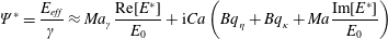 $$\begin{eqnarray}\unicode[STIX]{x1D6F9}^{\ast }=\frac{E_{eff}}{\unicode[STIX]{x1D6FE}}\approx Ma_{\unicode[STIX]{x1D6FE}}\frac{\text{Re}[E^{\ast }]}{E_{0}}+\text{i}Ca\left(Bq_{\unicode[STIX]{x1D702}}+Bq_{\unicode[STIX]{x1D705}}+Ma\frac{\text{Im}[E^{\ast }]}{E_{0}}\right)\end{eqnarray}$$
takes the place of $Ma_{\unicode[STIX]{x1D6FE}}=E_{0}/\unicode[STIX]{x1D6FE}$
in (4.71), since
$Ma_{\unicode[STIX]{x1D6FE}}=E_{0}/\unicode[STIX]{x1D6FE}$
in (4.71), since $\unicode[STIX]{x1D6FD}\ll \unicode[STIX]{x1D714}_{0}$
, where
$\unicode[STIX]{x1D6FD}\ll \unicode[STIX]{x1D714}_{0}$
, where $Ma$
and
$Ma$
and $Ma_{\unicode[STIX]{x1D6FE}}$
are defined in table 3, and
$Ma_{\unicode[STIX]{x1D6FE}}$
are defined in table 3, and
 $$\begin{eqnarray}Ca=\frac{\unicode[STIX]{x1D702}c}{\unicode[STIX]{x1D6FE}},\quad Bq_{\unicode[STIX]{x1D702}}=\frac{\unicode[STIX]{x1D702}_{s}k}{\unicode[STIX]{x1D702}},\quad Bq_{\unicode[STIX]{x1D705}}=\frac{\unicode[STIX]{x1D705}_{s}k}{\unicode[STIX]{x1D702}}.\end{eqnarray}$$
Equation (4.78) is the analogue of (4.43) for the mechanical response of oscillating bubbles.
The damping rate is a non-trivial function of $Ma_{\unicode[STIX]{x1D6FE}}$
,
$Ma_{\unicode[STIX]{x1D6FE}}$
, $Bq_{\unicode[STIX]{x1D702}}$
or
$Bq_{\unicode[STIX]{x1D702}}$
or $Bq_{\unicode[STIX]{x1D705}}$
in general, with limiting values of
$Bq_{\unicode[STIX]{x1D705}}$
in general, with limiting values of $\unicode[STIX]{x1D6FD}_{clean}$
(4.67) when
$\unicode[STIX]{x1D6FD}_{clean}$
(4.67) when $|\unicode[STIX]{x1D6F9}^{\ast }|\rightarrow 0$
and
$|\unicode[STIX]{x1D6F9}^{\ast }|\rightarrow 0$
and $\unicode[STIX]{x1D6FD}_{stiff}$
(4.73) when
$\unicode[STIX]{x1D6FD}_{stiff}$
(4.73) when $|\unicode[STIX]{x1D6F9}^{\ast }|\rightarrow \infty$
. The rate of damping therefore does not distinguish between the specific surfactant processes responsible for the damping. Measurements of a partially immobilized interface can at best be used to determine the lumped immobilization parameter
$|\unicode[STIX]{x1D6F9}^{\ast }|\rightarrow \infty$
. The rate of damping therefore does not distinguish between the specific surfactant processes responsible for the damping. Measurements of a partially immobilized interface can at best be used to determine the lumped immobilization parameter $\unicode[STIX]{x1D6F9}^{\ast }$
.
$\unicode[STIX]{x1D6F9}^{\ast }$
.
4.4 Thin films: surfactant dynamics affects thickness of coating
Thin fluid films are central to engineering and biophysical flows, most of which involve surfactants. Every blink or breath involves the dynamics of a tear film or the alveolar fluid film, and every stroke of a paintbrush leaves a thin liquid film that eventually dries. Industrial machinery is often coated with thin films of lubricant, and fibres, parts and products are coated by thin liquid films that are flowed over the objects. As with §§ 4.1–4.3, the effects of surface viscosity and Marangoni flows cannot always be neatly differentiated in many of these applications. In this section, we will quantify surfactant-covered thin film flows and highlight how the observable quantity (e.g. film thickness) relates to one or many ‘hidden’ surfactant variables.
4.4.1 Plate coating: the Landau–Levich–Derjaguin problem
Dip coating is perhaps the easiest way to deposit a thin liquid film on an object: dip the object in a liquid reservoir, then pull it out. The thickness $h$
of the entrained liquid layer depends on the velocity
$h$
of the entrained liquid layer depends on the velocity $V$
of the substrate, and the density, viscosity and surface tension of the liquid being drawn out (figure 20) as given by the classic Landau–Levich–Derjaguin (LLD) law,
$V$
of the substrate, and the density, viscosity and surface tension of the liquid being drawn out (figure 20) as given by the classic Landau–Levich–Derjaguin (LLD) law,
 $$\begin{eqnarray}\frac{h_{LLD}}{\ell _{c}}\approx 0.946\,Ca^{2/3},\end{eqnarray}$$
where
 $$\begin{eqnarray}\ell _{c}=\sqrt{\frac{\unicode[STIX]{x1D6FE}}{\unicode[STIX]{x1D70C}g}}\end{eqnarray}$$
is the capillary length (Landau & Levich Reference Landau and Levich1942; Quéré Reference Quéré1999), and $Ca=\unicode[STIX]{x1D702}V/\unicode[STIX]{x1D6FE}$
is the capillary number.
$Ca=\unicode[STIX]{x1D702}V/\unicode[STIX]{x1D6FE}$
is the capillary number.
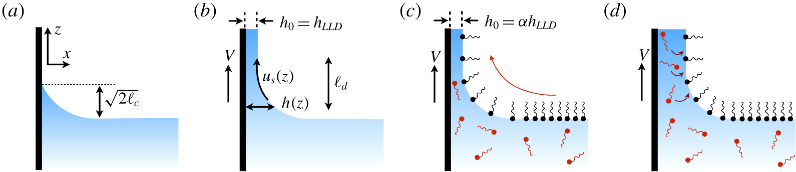
Figure 20. (a) A static meniscus form next to a stationary wall and the liquid level rises to a height $\sqrt{2}\ell _{c}$
. (b) When the wall is drawn upward, a film of liquid of asymptotic thickness
$\sqrt{2}\ell _{c}$
. (b) When the wall is drawn upward, a film of liquid of asymptotic thickness $h_{0}$
is entrained, and a dynamic meniscus connects the coating with the liquid reservoir. When the surface is clean, the LLD scaling gives
$h_{0}$
is entrained, and a dynamic meniscus connects the coating with the liquid reservoir. When the surface is clean, the LLD scaling gives $h_{0}\sim Ca^{2/3}\ell _{c}$
. (c) When surfactants occupy the liquid–air interface, Marangoni effects (and/or surface viscosity, see discussion) resist surface dilatation, drawing more fluid along with the moving plate. The coating is thicker by the factor
$h_{0}\sim Ca^{2/3}\ell _{c}$
. (c) When surfactants occupy the liquid–air interface, Marangoni effects (and/or surface viscosity, see discussion) resist surface dilatation, drawing more fluid along with the moving plate. The coating is thicker by the factor $\unicode[STIX]{x1D6FC}$
. (d) If the entrained film is thick enough, or if bulk concentration is large enough, surface concentration gradients are suppressed by adsorption of surfactant molecules to the interface, weakening the Marangoni effect.
$\unicode[STIX]{x1D6FC}$
. (d) If the entrained film is thick enough, or if bulk concentration is large enough, surface concentration gradients are suppressed by adsorption of surfactant molecules to the interface, weakening the Marangoni effect.
The LLD scaling follows from dividing the film into three regions: a film of uniform thickness coating the plate far above the reservoir, a static or undisturbed meniscus (figure 20
a), and an intermediate dynamic meniscus of length $\ell _{d}$
that smoothly matches the interfacial curvature between the uniform coating and the static meniscus (figure 20
b). Neglecting fluid inertia, the viscous stress in a dynamic meniscus of thickness
$\ell _{d}$
that smoothly matches the interfacial curvature between the uniform coating and the static meniscus (figure 20
b). Neglecting fluid inertia, the viscous stress in a dynamic meniscus of thickness $h$
scales with
$h$
scales with $\unicode[STIX]{x1D702}V/h^{2}$
, and balances the capillary stress, which is the gradient of the Laplace pressure (
$\unicode[STIX]{x1D702}V/h^{2}$
, and balances the capillary stress, which is the gradient of the Laplace pressure ( $\unicode[STIX]{x1D6FE}/\ell _{c}$
) along the dynamic meniscus of length
$\unicode[STIX]{x1D6FE}/\ell _{c}$
) along the dynamic meniscus of length $\ell _{d}$
 $$\begin{eqnarray}\frac{\unicode[STIX]{x1D702}V}{h^{2}}\sim \frac{\unicode[STIX]{x1D6FE}}{\ell _{c}\ell _{d}}.\end{eqnarray}$$
Near the liquid reservoir, the curvature of the dynamic meniscus must smoothly match to the static meniscus, which is set by the capillary length $\ell _{c}$
, giving
$\ell _{c}$
, giving
 $$\begin{eqnarray}\frac{1}{\ell _{c}}\sim \frac{h}{\ell _{d}^{2}}.\end{eqnarray}$$
Combining (4.82) and (4.83) to eliminate $\ell _{d}$
gives the
$\ell _{d}$
gives the $Ca^{2/3}$
scaling in the LLD law.
$Ca^{2/3}$
scaling in the LLD law.
The fluid being drawn out of the bath is rarely pure in most applications, and it has long been known that surfactants enhance the thickness $h_{0}$
of the film. Reverse Marangoni stresses and possibly surface rheological stresses immobilize the interface, dragging excess liquid along with the surface. In the following sections, we will outline recent studies that adapt the LLD approach to accommodate various surfactant processes, which first requires a description of the fluid dynamics of the entrained film.
$h_{0}$
of the film. Reverse Marangoni stresses and possibly surface rheological stresses immobilize the interface, dragging excess liquid along with the surface. In the following sections, we will outline recent studies that adapt the LLD approach to accommodate various surfactant processes, which first requires a description of the fluid dynamics of the entrained film.
For simplicity, we assume that the balance between viscous and capillary stresses dominate the dynamic meniscus. In particular, both inertia and gravity are weak, such that $\unicode[STIX]{x1D70C}V^{2}/h_{0}\ll \unicode[STIX]{x1D702}V/h_{0}^{2}$
and
$\unicode[STIX]{x1D70C}V^{2}/h_{0}\ll \unicode[STIX]{x1D702}V/h_{0}^{2}$
and $\unicode[STIX]{x1D70C}g\ll \unicode[STIX]{x1D702}V/h_{0}^{2}$
, where
$\unicode[STIX]{x1D70C}g\ll \unicode[STIX]{x1D702}V/h_{0}^{2}$
, where $V$
is the withdrawal velocity and
$V$
is the withdrawal velocity and $h_{0}$
is the film thickness. Under these assumptions, fluid does not drain to leading order: the film asymptotes to a uniform upward flow far from the reservoir. For sufficiently thin films (
$h_{0}$
is the film thickness. Under these assumptions, fluid does not drain to leading order: the film asymptotes to a uniform upward flow far from the reservoir. For sufficiently thin films ( $h_{0}\ll \ell _{c}$
), lubrication theory holds within the dynamic meniscus
$h_{0}\ll \ell _{c}$
), lubrication theory holds within the dynamic meniscus
 $$\begin{eqnarray}\unicode[STIX]{x1D702}\frac{\unicode[STIX]{x2202}^{2}u}{\unicode[STIX]{x2202}x^{2}}=\frac{\unicode[STIX]{x2202}p}{\unicode[STIX]{x2202}z},\quad \frac{\unicode[STIX]{x2202}p}{\unicode[STIX]{x2202}x}=0.\end{eqnarray}$$
Near the plate, the slope and curvature of the liquid surface $h(z)$
is small, and the Young–Laplace equation (2.6) gives the capillary pressure
$h(z)$
is small, and the Young–Laplace equation (2.6) gives the capillary pressure
 $$\begin{eqnarray}p_{c}\approx -\unicode[STIX]{x1D6FE}\frac{\text{d}^{2}h}{\text{d}z^{2}}.\end{eqnarray}$$
However, $\unicode[STIX]{x2202}p/\unicode[STIX]{x2202}x=0$
within the lubrication layer, and therefore bulk fluid pressure
$\unicode[STIX]{x2202}p/\unicode[STIX]{x2202}x=0$
within the lubrication layer, and therefore bulk fluid pressure $p$
is constant across the film, and equal to the local capillary pressure
$p$
is constant across the film, and equal to the local capillary pressure $p_{c}(z)$
. Substituting
$p_{c}(z)$
. Substituting $p(z)=p_{c}(z)$
in (4.84) and solving with boundary conditions
$p(z)=p_{c}(z)$
in (4.84) and solving with boundary conditions $u(x=0)=V$
and
$u(x=0)=V$
and $u(x=h)=u_{s}$
gives
$u(x=h)=u_{s}$
gives
 $$\begin{eqnarray}u(x,z)=-\frac{\unicode[STIX]{x1D6FE}}{2\unicode[STIX]{x1D702}}\frac{\text{d}^{3}h}{\text{d}z^{3}}(x^{2}-xh)+(u_{s}-V)\frac{x}{h}+V.\end{eqnarray}$$
Note that the surface velocity $u_{s}(z)$
and film thickness
$u_{s}(z)$
and film thickness $h(z)$
are yet unknown.
$h(z)$
are yet unknown.
Since gravitational drainage is negligible, $h(z)$
follows from mass conservation (
$h(z)$
follows from mass conservation ( $\int _{0}^{h}u\,\text{d}x=Vh_{0}$
), to give
$\int _{0}^{h}u\,\text{d}x=Vh_{0}$
), to give
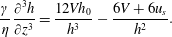 $$\begin{eqnarray}\frac{\unicode[STIX]{x1D6FE}}{\unicode[STIX]{x1D702}}\frac{\unicode[STIX]{x2202}^{3}h}{\unicode[STIX]{x2202}z^{3}}=\frac{12Vh_{0}}{h^{3}}-\frac{6V+6u_{s}}{h^{2}}.\end{eqnarray}$$
The surface velocity $u_{s}(z)$
is then determined by the interfacial stress condition. For a surfactant-free film, imposing
$u_{s}(z)$
is then determined by the interfacial stress condition. For a surfactant-free film, imposing $\unicode[STIX]{x1D702}\unicode[STIX]{x2202}u/\unicode[STIX]{x2202}x|_{x=h}=0$
in (4.86) and substituting (4.87) gives
$\unicode[STIX]{x1D702}\unicode[STIX]{x2202}u/\unicode[STIX]{x2202}x|_{x=h}=0$
in (4.86) and substituting (4.87) gives
 $$\begin{eqnarray}\frac{u_{s}}{V}=\frac{3}{2}\frac{h_{0}}{h}-\frac{1}{2}.\end{eqnarray}$$
Notably, a stagnation point appears at $h(z)=3h_{0}$
, meaning that the surface velocity is directed along the plate motion for only a section of the dynamic meniscus. Surfactants modify this stagnation point, enabling more fluid to be drawn.
$h(z)=3h_{0}$
, meaning that the surface velocity is directed along the plate motion for only a section of the dynamic meniscus. Surfactants modify this stagnation point, enabling more fluid to be drawn.
Substituting (4.88) in (4.87) gives the LLD equation
 $$\begin{eqnarray}\frac{\unicode[STIX]{x1D6FE}}{\unicode[STIX]{x1D702}}h^{\prime \prime \prime }=\frac{3V}{h^{3}}(h_{0}-h),\end{eqnarray}$$
where primes represent derivatives in $z$
. In dimensionless variables, (4.89) becomes
$z$
. In dimensionless variables, (4.89) becomes
 $$\begin{eqnarray}\tilde{h}^{3}\tilde{h}^{\prime \prime \prime }=1-\tilde{h},\end{eqnarray}$$
where $\tilde{h}=h/h_{0}$
and
$\tilde{h}=h/h_{0}$
and $\tilde{z}=z/\ell _{d}$
, and the dynamic meniscus length is
$\tilde{z}=z/\ell _{d}$
, and the dynamic meniscus length is
 $$\begin{eqnarray}\ell _{d}=\frac{h_{0}}{(3\,Ca)^{1/3}}.\end{eqnarray}$$
Far from the reservoir, $\tilde{h}(\infty )\rightarrow 1$
,
$\tilde{h}(\infty )\rightarrow 1$
, $\tilde{h}^{\prime }(\infty )\rightarrow 0$
and
$\tilde{h}^{\prime }(\infty )\rightarrow 0$
and $\tilde{h}^{\prime \prime }(\infty )\rightarrow 0$
.
$\tilde{h}^{\prime \prime }(\infty )\rightarrow 0$
.
Landau & Levich (Reference Landau and Levich1942) realized that $\tilde{h}^{\prime \prime }$
must asymptotically match the curvature of the static meniscus near the reservoir. Using the Young–Laplace law and assuming zero contact angle, the static meniscus has height
$\tilde{h}^{\prime \prime }$
must asymptotically match the curvature of the static meniscus near the reservoir. Using the Young–Laplace law and assuming zero contact angle, the static meniscus has height $\sqrt{2}\ell _{c}$
and curvature
$\sqrt{2}\ell _{c}$
and curvature $\sqrt{2}/\ell _{c}$
. In dimensionless terms, this inner boundary condition on (4.90) becomes
$\sqrt{2}/\ell _{c}$
. In dimensionless terms, this inner boundary condition on (4.90) becomes
 $$\begin{eqnarray}\tilde{h}^{\prime \prime }=\frac{\sqrt{2}h_{0}}{\ell _{c}}\left(\frac{\unicode[STIX]{x1D6FE}}{3\unicode[STIX]{x1D702}V}\right)^{2/3}\approx 0.64,\end{eqnarray}$$
where the constant is found by numerically integrating (4.90). Rearranging (4.92) for the residual thickness $h_{0}$
then gives the classic LLD law (4.80).
$h_{0}$
then gives the classic LLD law (4.80).
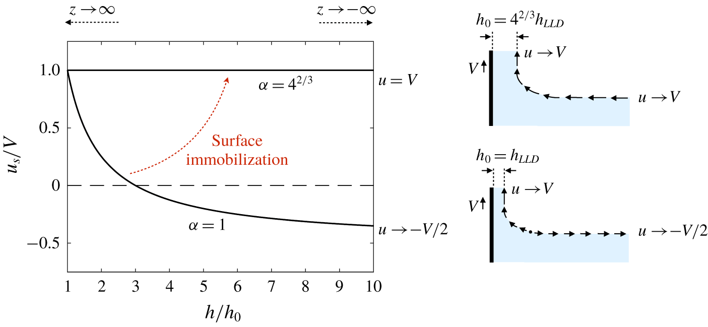
Figure 21. Surface velocity of the entrained film. The surface flow has a stagnation point for a clean interface ( $\unicode[STIX]{x1D6FC}=1$
) beyond which the fluid flow is in the direction opposite to that of the plate. With increasing
$\unicode[STIX]{x1D6FC}=1$
) beyond which the fluid flow is in the direction opposite to that of the plate. With increasing $\unicode[STIX]{x1D6FC}$
, the surface is immobilised until a maximal value of
$\unicode[STIX]{x1D6FC}$
, the surface is immobilised until a maximal value of $\unicode[STIX]{x1D6FC}=4^{2/3}$
, when the interface is surface incompressible and is drawn at the same velocity as the plate everywhere.
$\unicode[STIX]{x1D6FC}=4^{2/3}$
, when the interface is surface incompressible and is drawn at the same velocity as the plate everywhere.
In anticipation of the immobilizing effect of surfactants, we calculate the extreme case of complete surface immobilization. An incompressible surface has $u_{s}=V$
, and (4.87) becomes
$u_{s}=V$
, and (4.87) becomes
 $$\begin{eqnarray}\frac{\unicode[STIX]{x1D6FE}}{\unicode[STIX]{x1D702}}h^{\prime \prime \prime }=\frac{12V}{h^{3}}(h_{0}-h),\end{eqnarray}$$
Comparing (4.93) with (4.89) reveals this limit to be identical to the standard LLD problem, but with a modified dynamic meniscus length
 $$\begin{eqnarray}\ell _{d}^{immob}=\frac{h_{0}}{(12\,Ca)^{1/3}}.\end{eqnarray}$$
In other words, the dimensionless problem and the matching proceeds exactly like for LLD, but with a capillary number that four times larger, thereby modifying this LLD scaling to
 $$\begin{eqnarray}\frac{h_{0}^{immob}}{\ell _{c}}\approx 0.946\,(4Ca)^{2/3}=4^{2/3}\frac{h_{LLD}}{\ell _{c}}.\end{eqnarray}$$
An incompressible interface entrains more fluid as the plate is withdrawn, increasing the film thickness up to $4^{2/3}$
more than a fully mobile interface (figure 21). In what follows, we will treat specific surfactant processes based on illustrative works in dip coating (Park Reference Park1991; Quéré Reference Quéré1999; Shen et al.
Reference Shen, Gleason, McKinley and Stone2002; Scheid et al.
Reference Scheid, Delacotte, Dollet, Rio, Restagno, van Nierop, Cantat, Langevin and Stone2010), each of which reveals a similar transition between the clean and immobilized limits.
$4^{2/3}$
more than a fully mobile interface (figure 21). In what follows, we will treat specific surfactant processes based on illustrative works in dip coating (Park Reference Park1991; Quéré Reference Quéré1999; Shen et al.
Reference Shen, Gleason, McKinley and Stone2002; Scheid et al.
Reference Scheid, Delacotte, Dollet, Rio, Restagno, van Nierop, Cantat, Langevin and Stone2010), each of which reveals a similar transition between the clean and immobilized limits.
4.4.2 Insoluble and surface-inviscid surfactant
Surfactants give rise to Marangoni and surface-viscous forces that resist interfacial stretching. The Boussinesq–Scriven equation (3.94) modifies the interfacial stress balance to
 $$\begin{eqnarray}\frac{\unicode[STIX]{x2202}\unicode[STIX]{x1D6FE}}{\unicode[STIX]{x2202}z}+(\unicode[STIX]{x1D702}_{s}+\unicode[STIX]{x1D705}_{s})\frac{\unicode[STIX]{x2202}^{2}u_{s}}{\unicode[STIX]{x2202}z^{2}}=\unicode[STIX]{x1D702}\left.\frac{\unicode[STIX]{x2202}u}{\unicode[STIX]{x2202}x}\right|_{x=h}=\unicode[STIX]{x1D702}\left(-\frac{6Vh_{0}}{h^{2}}+\frac{2V+4u_{s}}{h}\right),\end{eqnarray}$$
where $u(x,z)$
follows from (4.86) and (4.87). We will first consider insoluble surfactants that are surface inviscid, so that
$u(x,z)$
follows from (4.86) and (4.87). We will first consider insoluble surfactants that are surface inviscid, so that $\unicode[STIX]{x1D702}_{s}=\unicode[STIX]{x1D705}_{s}=0$
. Surface fluid flows establish gradients in
$\unicode[STIX]{x1D702}_{s}=\unicode[STIX]{x1D705}_{s}=0$
. Surface fluid flows establish gradients in $\unicode[STIX]{x1D6E4}$
, which exert reverse Marangoni stresses. Without surfactant exchange, surface diffusion is the only mechanism to relax gradients in
$\unicode[STIX]{x1D6E4}$
, which exert reverse Marangoni stresses. Without surfactant exchange, surface diffusion is the only mechanism to relax gradients in $\unicode[STIX]{x1D6FE}(\unicode[STIX]{x1D6E4})$
. Perturbing the surface concentration via
$\unicode[STIX]{x1D6FE}(\unicode[STIX]{x1D6E4})$
. Perturbing the surface concentration via $\unicode[STIX]{x1D6E4}(z)=\unicode[STIX]{x1D6E4}_{0}+\unicode[STIX]{x1D6FF}\unicode[STIX]{x1D6E4}(z)$
, the steady-state surface conservation equation (3.10) becomes
$\unicode[STIX]{x1D6E4}(z)=\unicode[STIX]{x1D6E4}_{0}+\unicode[STIX]{x1D6FF}\unicode[STIX]{x1D6E4}(z)$
, the steady-state surface conservation equation (3.10) becomes
 $$\begin{eqnarray}\unicode[STIX]{x1D6E4}_{0}\frac{\unicode[STIX]{x2202}u_{s}}{\unicode[STIX]{x2202}z}=D_{s}\frac{\unicode[STIX]{x2202}^{2}(\unicode[STIX]{x1D6FF}\unicode[STIX]{x1D6E4})}{\unicode[STIX]{x2202}z^{2}}.\end{eqnarray}$$
Integrating (4.97) and imposing $\unicode[STIX]{x2202}\unicode[STIX]{x1D6E4}/\unicode[STIX]{x2202}z(z\rightarrow \infty )\rightarrow 0$
and
$\unicode[STIX]{x2202}\unicode[STIX]{x1D6E4}/\unicode[STIX]{x2202}z(z\rightarrow \infty )\rightarrow 0$
and $u_{s}(z\rightarrow \infty )\rightarrow V$
gives
$u_{s}(z\rightarrow \infty )\rightarrow V$
gives
 $$\begin{eqnarray}\frac{\unicode[STIX]{x2202}(\unicode[STIX]{x1D6FF}\unicode[STIX]{x1D6E4})}{\unicode[STIX]{x2202}z}=\frac{\unicode[STIX]{x1D6E4}_{0}}{D_{s}}(u_{s}-V).\end{eqnarray}$$
The Marangoni stress is then given by
 $$\begin{eqnarray}\frac{\unicode[STIX]{x2202}\unicode[STIX]{x1D6FE}}{\unicode[STIX]{x2202}z}=-\frac{E_{0}}{\unicode[STIX]{x1D6E4}_{0}}\frac{\unicode[STIX]{x2202}\unicode[STIX]{x1D6FF}\unicode[STIX]{x1D6E4}}{\unicode[STIX]{x2202}z}=-\frac{E_{0}}{D_{s}}(u_{s}-V).\end{eqnarray}$$
Substituting into the interfacial stress balance (4.96) with $\unicode[STIX]{x1D702}_{s}=\unicode[STIX]{x1D705}_{s}=0$
and non-dimensionalizing gives
$\unicode[STIX]{x1D702}_{s}=\unicode[STIX]{x1D705}_{s}=0$
and non-dimensionalizing gives
 $$\begin{eqnarray}Ma_{D}(1-\tilde{u} _{s})=-\frac{6}{\tilde{h}^{2}}+\frac{2+4\tilde{u} _{s}}{\tilde{h}},\end{eqnarray}$$
where the surface diffusive Marangoni number (table 3) is:
 $$\begin{eqnarray}Ma_{D}=\frac{E_{0}h_{0}}{D_{s}\unicode[STIX]{x1D702}}=\frac{E_{0}}{\unicode[STIX]{x1D702}V}\times \frac{Vh_{0}}{D_{s}}=Ma\times Pe_{s}.\end{eqnarray}$$
When $Ma_{D}\gg 1$
, the interface is immobilized relative to the moving plate, and (4.100) gives
$Ma_{D}\gg 1$
, the interface is immobilized relative to the moving plate, and (4.100) gives $\tilde{u} _{s}\rightarrow 1$
, or
$\tilde{u} _{s}\rightarrow 1$
, or $u_{s}\rightarrow V$
. This surface immobilization occurs when the Marangoni modulus is large or surface diffusivity is weak. By contrast, weak Marangoni flows or strong surface diffusion (
$u_{s}\rightarrow V$
. This surface immobilization occurs when the Marangoni modulus is large or surface diffusivity is weak. By contrast, weak Marangoni flows or strong surface diffusion ( $Ma_{D}\ll 1$
) recovers the
$Ma_{D}\ll 1$
) recovers the $u_{s}$
corresponding to clean surfaces (4.88).
$u_{s}$
corresponding to clean surfaces (4.88).
The film thickness equation (4.87) for an inviscid, insoluble surfactant, using (4.100) for $u_{s}$
, is
$u_{s}$
, is
 $$\begin{eqnarray}\tilde{h}^{3}\tilde{h}^{\prime \prime \prime }=(1-\tilde{h})\left(1+\frac{3\tilde{h}Ma_{D}}{4+\tilde{h}Ma_{D}}\right).\end{eqnarray}$$
As $Ma_{D}\rightarrow 0$
, (4.102) is identical to the classic LLD equation for a clean interface (4.90). For strong immobilization as
$Ma_{D}\rightarrow 0$
, (4.102) is identical to the classic LLD equation for a clean interface (4.90). For strong immobilization as $Ma_{D}\rightarrow \infty$
, the right-hand side increases fourfold, amplifying the apparent capillary number fourfold, and increasing the film thickness by
$Ma_{D}\rightarrow \infty$
, the right-hand side increases fourfold, amplifying the apparent capillary number fourfold, and increasing the film thickness by $4^{2/3}$
(Park Reference Park1991; Quéré Reference Quéré1999).
$4^{2/3}$
(Park Reference Park1991; Quéré Reference Quéré1999).
4.4.3 Soluble and/or surface-viscous surfactant
Adsorption/desorption weakens the Marangoni effect, and reduces the thickening factor $\unicode[STIX]{x1D6FC}=h/h_{LLD}$
(Ou Ramdane & Quéré Reference Ou Ramdane and Quéré1997). However, as with oscillating bubbles (§ 4.2.2) and wave damping (§ 4.3), the distinct effects of adsorption/desorption and intrinsic surface viscosities are not easy to tease apart. The role of surface viscosity in dip coating has only recently gained attention (Scheid et al.
Reference Scheid, Delacotte, Dollet, Rio, Restagno, van Nierop, Cantat, Langevin and Stone2010; Delacotte et al.
Reference Delacotte, Montel, Restagno, Scheid, Dollet, Stone, Langevin and Rio2012; Seiwert et al.
Reference Seiwert, Dollet and Cantat2014) in systems with negligible Marangoni forces; e.g. when rapid adsorption/desorption eliminates surface tension gradients.
$\unicode[STIX]{x1D6FC}=h/h_{LLD}$
(Ou Ramdane & Quéré Reference Ou Ramdane and Quéré1997). However, as with oscillating bubbles (§ 4.2.2) and wave damping (§ 4.3), the distinct effects of adsorption/desorption and intrinsic surface viscosities are not easy to tease apart. The role of surface viscosity in dip coating has only recently gained attention (Scheid et al.
Reference Scheid, Delacotte, Dollet, Rio, Restagno, van Nierop, Cantat, Langevin and Stone2010; Delacotte et al.
Reference Delacotte, Montel, Restagno, Scheid, Dollet, Stone, Langevin and Rio2012; Seiwert et al.
Reference Seiwert, Dollet and Cantat2014) in systems with negligible Marangoni forces; e.g. when rapid adsorption/desorption eliminates surface tension gradients.
Assuming surface diffusion to be negligible, gradients in $\unicode[STIX]{x1D6FE}(\unicode[STIX]{x1D6E4})$
are governed by the balance of flow and adsorption (§ 3.2)
$\unicode[STIX]{x1D6FE}(\unicode[STIX]{x1D6E4})$
are governed by the balance of flow and adsorption (§ 3.2)
 $$\begin{eqnarray}\unicode[STIX]{x1D6E4}_{0}\frac{\unicode[STIX]{x2202}u_{s}}{\unicode[STIX]{x2202}z}=-\frac{\unicode[STIX]{x1D6FF}\unicode[STIX]{x1D6E4}}{\unicode[STIX]{x1D70F}_{s}}.\end{eqnarray}$$
Taking perturbations $\unicode[STIX]{x1D6FF}\unicode[STIX]{x1D6E4}$
from equilibrium
$\unicode[STIX]{x1D6FF}\unicode[STIX]{x1D6E4}$
from equilibrium $\unicode[STIX]{x1D6E4}_{0}$
to be small gives a Marangoni stress
$\unicode[STIX]{x1D6E4}_{0}$
to be small gives a Marangoni stress
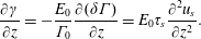 $$\begin{eqnarray}\frac{\unicode[STIX]{x2202}\unicode[STIX]{x1D6FE}}{\unicode[STIX]{x2202}z}=-\frac{E_{0}}{\unicode[STIX]{x1D6E4}_{0}}\frac{\unicode[STIX]{x2202}(\unicode[STIX]{x1D6FF}\unicode[STIX]{x1D6E4})}{\unicode[STIX]{x2202}z}=E_{0}\unicode[STIX]{x1D70F}_{s}\frac{\unicode[STIX]{x2202}^{2}u_{s}}{\unicode[STIX]{x2202}z^{2}}.\end{eqnarray}$$
Substituting (4.103) in the interfacial stress condition (4.96) gives
 $$\begin{eqnarray}\left(\frac{E_{0}\unicode[STIX]{x1D70F}_{s}+\unicode[STIX]{x1D702}_{s}+\unicode[STIX]{x1D705}_{s}}{\unicode[STIX]{x1D702}}\right)\frac{\unicode[STIX]{x2202}^{2}u_{s}}{\unicode[STIX]{x2202}z^{2}}=-\frac{6Vh_{0}}{h^{2}}+\frac{2V+4u_{s}}{h}.\end{eqnarray}$$
Non-dimensionalizing over $h_{0}$
,
$h_{0}$
, $V$
and
$V$
and $\ell _{d}=(3\,Ca)^{-1/3}h_{0}$
for
$\ell _{d}=(3\,Ca)^{-1/3}h_{0}$
for $h(z)$
,
$h(z)$
, $u_{s}(z)$
and
$u_{s}(z)$
and $z$
gives
$z$
gives
 $$\begin{eqnarray}\tilde{\unicode[STIX]{x1D6F9}}\frac{\unicode[STIX]{x2202}^{2}\tilde{u} _{s}}{\unicode[STIX]{x2202}z^{2}}=-\frac{6}{\tilde{h}^{2}}+\frac{2+4\tilde{u} _{s}}{\tilde{h}},\end{eqnarray}$$
where
 $$\begin{eqnarray}\tilde{\unicode[STIX]{x1D6F9}}=\frac{(3Ca)^{2/3}\unicode[STIX]{x1D6F9}\ell _{c}}{h_{0}},\end{eqnarray}$$
and $\unicode[STIX]{x1D6F9}$
is the surface-immobilization parameter, described in § 3.4.3
$\unicode[STIX]{x1D6F9}$
is the surface-immobilization parameter, described in § 3.4.3
 $$\begin{eqnarray}\unicode[STIX]{x1D6F9}=\frac{E_{0}\unicode[STIX]{x1D70F}_{s}+\unicode[STIX]{x1D702}_{s}+\unicode[STIX]{x1D705}_{s}}{\unicode[STIX]{x1D702}\ell _{c}}=Ma_{K}+Bq_{\unicode[STIX]{x1D702}}+Bq_{\unicode[STIX]{x1D705}}.\end{eqnarray}$$
If $E_{0}$
,
$E_{0}$
, $\unicode[STIX]{x1D70F}_{s}$
,
$\unicode[STIX]{x1D70F}_{s}$
, $\unicode[STIX]{x1D702}_{s}$
and
$\unicode[STIX]{x1D702}_{s}$
and $\unicode[STIX]{x1D705}_{s}$
are known separately, (4.106) can be solved numerically along with the film thickness equation (4.87) for arbitrary values of
$\unicode[STIX]{x1D705}_{s}$
are known separately, (4.106) can be solved numerically along with the film thickness equation (4.87) for arbitrary values of $\unicode[STIX]{x1D6F9}$
(Scheid et al.
Reference Scheid, Delacotte, Dollet, Rio, Restagno, van Nierop, Cantat, Langevin and Stone2010). The limits of large and small
$\unicode[STIX]{x1D6F9}$
(Scheid et al.
Reference Scheid, Delacotte, Dollet, Rio, Restagno, van Nierop, Cantat, Langevin and Stone2010). The limits of large and small $\unicode[STIX]{x1D6F9}$
are easy to interpret: the surface is fully mobile as
$\unicode[STIX]{x1D6F9}$
are easy to interpret: the surface is fully mobile as $\unicode[STIX]{x1D6F9}\rightarrow 0$
, recovering the classic LLD solution. By contrast, the interface is immobilized as
$\unicode[STIX]{x1D6F9}\rightarrow 0$
, recovering the classic LLD solution. By contrast, the interface is immobilized as $\unicode[STIX]{x1D6F9}\rightarrow \infty$
, in which case
$\unicode[STIX]{x1D6F9}\rightarrow \infty$
, in which case $u_{s}\approx V$
everywhere. The same factor of
$u_{s}\approx V$
everywhere. The same factor of $4$
found in the
$4$
found in the $Ma_{D}\rightarrow \infty$
limit of (4.102) appears in the LLD equation, and the film thickness increases by
$Ma_{D}\rightarrow \infty$
limit of (4.102) appears in the LLD equation, and the film thickness increases by $4^{2/3}$
.
$4^{2/3}$
.
Measured film thickness depends on the lumped parameter $\unicode[STIX]{x1D6F9}$
and does not distinguish between three distinct phenomena – surface shear viscosity, surface dilatational viscosity and apparent dilational viscosity due to adsorption/desorption (§ 3.4.3). More information, e.g. from complementary experiments, would be required to deconvolve the impact of each.
$\unicode[STIX]{x1D6F9}$
and does not distinguish between three distinct phenomena – surface shear viscosity, surface dilatational viscosity and apparent dilational viscosity due to adsorption/desorption (§ 3.4.3). More information, e.g. from complementary experiments, would be required to deconvolve the impact of each.
It may also be possible to suppress one surfactant process to isolate the effect of another in specific systems. For example, intrinsic surface viscosity becomes the dominant immobilizing component when $Bq\gtrsim Ma_{K}$
. The Marangoni contribution to immobilization is weakest when adsorption/desorption is fast: gradients in
$Bq\gtrsim Ma_{K}$
. The Marangoni contribution to immobilization is weakest when adsorption/desorption is fast: gradients in $\unicode[STIX]{x1D6E4}$
are small if
$\unicode[STIX]{x1D6E4}$
are small if $\unicode[STIX]{x1D70F}_{s}\ll \unicode[STIX]{x1D70F}_{flow}$
, so that
$\unicode[STIX]{x1D70F}_{s}\ll \unicode[STIX]{x1D70F}_{flow}$
, so that
 $$\begin{eqnarray}Ma_{K}=\frac{E_{0}}{\unicode[STIX]{x1D702}V}\times \frac{V\unicode[STIX]{x1D70F}_{s}}{\ell _{c}}=Ma\times \frac{\unicode[STIX]{x1D70F}_{s}}{\unicode[STIX]{x1D70F}_{flow}}\ll 1.\end{eqnarray}$$
This condition, however, does not account for finite subphase depth and the availability of surfactant molecules in the thin film. Effective surfactant exchange requires the film to be thicker than the depletion depth $L_{d}=\unicode[STIX]{x2202}\unicode[STIX]{x1D6E4}/\unicode[STIX]{x2202}C_{s}$
(§ 3.2), so as to not be ‘confined’ (Quéré Reference Quéré1999; Delacotte et al.
Reference Delacotte, Montel, Restagno, Scheid, Dollet, Stone, Langevin and Rio2012) by the lack of sufficient dissolved molecules. Suppressing Marangoni flows therefore requires large surfactant concentrations (so
$L_{d}=\unicode[STIX]{x2202}\unicode[STIX]{x1D6E4}/\unicode[STIX]{x2202}C_{s}$
(§ 3.2), so as to not be ‘confined’ (Quéré Reference Quéré1999; Delacotte et al.
Reference Delacotte, Montel, Restagno, Scheid, Dollet, Stone, Langevin and Rio2012) by the lack of sufficient dissolved molecules. Suppressing Marangoni flows therefore requires large surfactant concentrations (so $L_{d}$
is small), large withdrawing velocities (so
$L_{d}$
is small), large withdrawing velocities (so $h_{0}$
is large) and elimination of energetic barriers to adsorption (so
$h_{0}$
is large) and elimination of energetic barriers to adsorption (so $\unicode[STIX]{x1D70F}_{s}$
is small). Following this strategy, Delacotte et al. (Reference Delacotte, Montel, Restagno, Scheid, Dollet, Stone, Langevin and Rio2012) measured enhanced film thickness in unconfined films despite rapid adsorption, suggesting that surface viscosity does indeed play a role in immobilizing interfaces. However, the two surface viscosities
$\unicode[STIX]{x1D70F}_{s}$
is small). Following this strategy, Delacotte et al. (Reference Delacotte, Montel, Restagno, Scheid, Dollet, Stone, Langevin and Rio2012) measured enhanced film thickness in unconfined films despite rapid adsorption, suggesting that surface viscosity does indeed play a role in immobilizing interfaces. However, the two surface viscosities $\unicode[STIX]{x1D702}_{s}$
and
$\unicode[STIX]{x1D702}_{s}$
and $\unicode[STIX]{x1D705}_{s}$
still remain indistinguishable in 1-D surface deformations.
$\unicode[STIX]{x1D705}_{s}$
still remain indistinguishable in 1-D surface deformations.
Finally, the presence of micelles at high bulk surfactant concentrations influences thickness of the coating in non-trivial ways. Above the CMC, micelles dissociate to maintain a reservoir of free monomers, thereby eliminating diffusion limitation to adsorption. Bulk concentrations above the CMC thus lead to a thinner coating, as Marangoni flows are suppressed and the interface is ‘remobilized’ (Stebe & Maldarelli Reference Stebe and Maldarelli1994, see also § 4.1.2). However, micelles may dissociate at time scales comparable to or slower than the bulk diffusion time at very high concentrations, thereby depleting the bulk of free monomers and enhancing the Marangoni effect, which again leads to a thicker entrained film (Shen et al. Reference Shen, Gleason, McKinley and Stone2002).
4.4.4 Thin-film drainage
Gravitational drainage is negligible in the LLD problem, and fluid flow is driven entirely by capillary pressure. For illustration and completion, we will briefly examine one case where gravity drives thin-film flow. Approximating the flow in a thin film draining down a vertical wall using lubrication theory, the velocity $u(x,z,t)$
obeys
$u(x,z,t)$
obeys
 $$\begin{eqnarray}\unicode[STIX]{x1D702}\frac{\unicode[STIX]{x2202}^{2}u}{\unicode[STIX]{x2202}x^{2}}=-\unicode[STIX]{x1D70C}g,\end{eqnarray}$$
where $z$
is positive downward, and
$z$
is positive downward, and $x$
is perpendicular to gravity. Solving with a no-slip wall at
$x$
is perpendicular to gravity. Solving with a no-slip wall at $x=0$
and a (yet unknown) surface velocity
$x=0$
and a (yet unknown) surface velocity $u_{s}(z,t)$
, the fluid velocity is
$u_{s}(z,t)$
, the fluid velocity is
 $$\begin{eqnarray}u(x,z,t)=-\frac{\unicode[STIX]{x1D70C}g}{2\unicode[STIX]{x1D702}}(x^{2}-hx)+\frac{xu_{s}}{h}.\end{eqnarray}$$
Conservation of mass requires
 $$\begin{eqnarray}\frac{\unicode[STIX]{x2202}h}{\unicode[STIX]{x2202}t}+\frac{\unicode[STIX]{x2202}Q}{\unicode[STIX]{x2202}z}=0,\end{eqnarray}$$
where $Q(z,t)=\int _{0}^{h}u(x,z,t)\,\text{d}x$
is the vertical flux. Substituting (4.111) in (4.112) gives the film thickness equation
$Q(z,t)=\int _{0}^{h}u(x,z,t)\,\text{d}x$
is the vertical flux. Substituting (4.111) in (4.112) gives the film thickness equation
 $$\begin{eqnarray}h_{t}+\frac{\unicode[STIX]{x1D70C}g}{4\unicode[STIX]{x1D702}}h^{2}h^{\prime }+\frac{(hu_{s})^{\prime }}{2}=0,\end{eqnarray}$$
where primes represent $z$
derivatives, and the subscript
$z$
derivatives, and the subscript $t$
denotes time derivatives.
$t$
denotes time derivatives.
A clean fluid interface is stress free, and enforcing this at $x=h$
in (4.111) gives
$x=h$
in (4.111) gives
 $$\begin{eqnarray}u_{s}=\frac{\unicode[STIX]{x1D70C}gh^{2}}{2\unicode[STIX]{x1D702}}.\end{eqnarray}$$
Substituting (4.114) in (4.113) gives the evolution equation for a clean fluid film draining under gravity,
 $$\begin{eqnarray}h_{t}+\frac{\unicode[STIX]{x1D70C}g}{\unicode[STIX]{x1D702}}h^{2}h^{\prime }=0.\end{eqnarray}$$
By contrast, surfactant processes resist interfacial deformation, which modifies $u_{s}$
. Rather than explicitly treating surface rheology and transport, we will consider the extreme case when the surface is immobilized due to some combination of reverse Marangoni flow and surface-viscous resistance. Setting
$u_{s}$
. Rather than explicitly treating surface rheology and transport, we will consider the extreme case when the surface is immobilized due to some combination of reverse Marangoni flow and surface-viscous resistance. Setting $u_{s}=0$
in (4.113) gives
$u_{s}=0$
in (4.113) gives
 $$\begin{eqnarray}h_{t}+\frac{\unicode[STIX]{x1D70C}g}{4\unicode[STIX]{x1D702}}h^{2}h^{\prime }=0.\end{eqnarray}$$
Notably, the same factor of $4$
between the stress-free interface and the immobile interface appears here, as in the LLD problems (4.95).
$4$
between the stress-free interface and the immobile interface appears here, as in the LLD problems (4.95).
To solve the appropriate film equation, we use $R$
as a system-specific length scale (such as length of the plate) in the flow direction. Non-dimensionalizing over
$R$
as a system-specific length scale (such as length of the plate) in the flow direction. Non-dimensionalizing over $R$
,
$R$
, $h_{0}$
and
$h_{0}$
and $\unicode[STIX]{x1D702}R/(\unicode[STIX]{x1D70C}gh_{0}^{2})$
for
$\unicode[STIX]{x1D702}R/(\unicode[STIX]{x1D70C}gh_{0}^{2})$
for $z$
,
$z$
, $h$
and
$h$
and $t$
, respectively, gives
$t$
, respectively, gives
 $$\begin{eqnarray}\tilde{h}_{t}+\frac{1}{\unicode[STIX]{x1D6FD}}\tilde{h}^{2}\tilde{h}^{\prime }=0,\end{eqnarray}$$
where $\unicode[STIX]{x1D6FD}=1$
for a clean surface (4.115) and
$\unicode[STIX]{x1D6FD}=1$
for a clean surface (4.115) and $\unicode[STIX]{x1D6FD}=4$
for an immobile surface (4.116). The film thickness obeys a similarity solution,
$\unicode[STIX]{x1D6FD}=4$
for an immobile surface (4.116). The film thickness obeys a similarity solution, $h=F(\unicode[STIX]{x1D701})$
, where
$h=F(\unicode[STIX]{x1D701})$
, where $\unicode[STIX]{x1D701}=\sqrt{\tilde{z}/\tilde{t}}$
, and
$\unicode[STIX]{x1D701}=\sqrt{\tilde{z}/\tilde{t}}$
, and $F$
obeys
$F$
obeys
 $$\begin{eqnarray}F^{\prime }F^{2}-\unicode[STIX]{x1D6FD}\unicode[STIX]{x1D701}^{2}F^{\prime }=0,\end{eqnarray}$$
with solution $F(\unicode[STIX]{x1D701})=\sqrt{\unicode[STIX]{x1D6FD}}\unicode[STIX]{x1D701}$
. The dimensional film thickness is then
$F(\unicode[STIX]{x1D701})=\sqrt{\unicode[STIX]{x1D6FD}}\unicode[STIX]{x1D701}$
. The dimensional film thickness is then
 $$\begin{eqnarray}h(z,t)=\sqrt{\frac{\unicode[STIX]{x1D6FD}\unicode[STIX]{x1D702}z}{\unicode[STIX]{x1D70C}gt}}.\end{eqnarray}$$
The clean interface limit ( $\unicode[STIX]{x1D6FD}=1$
) recovers the classic Jeffreys solution (Jeffreys Reference Jeffreys1930). More generally, the
$\unicode[STIX]{x1D6FD}=1$
) recovers the classic Jeffreys solution (Jeffreys Reference Jeffreys1930). More generally, the $h\sim t^{-1/2}$
scaling persists even with surfactant. Drainage takes longer with surfactant, however, and the film is
$h\sim t^{-1/2}$
scaling persists even with surfactant. Drainage takes longer with surfactant, however, and the film is $\unicode[STIX]{x1D6FD}^{1/2}$
or twice as thick when the surface is completely immobile. Surface viscosity, Marangoni flows or some non-trivial combination acts to retard surface flow, thereby slowing film drainage. This effect is responsible in part for the long lives of soapy bubbles and foams (§ 4.5), and the increased coalescence time of surfactant-covered bubbles.
$\unicode[STIX]{x1D6FD}^{1/2}$
or twice as thick when the surface is completely immobile. Surface viscosity, Marangoni flows or some non-trivial combination acts to retard surface flow, thereby slowing film drainage. This effect is responsible in part for the long lives of soapy bubbles and foams (§ 4.5), and the increased coalescence time of surfactant-covered bubbles.
Bhamla et al. (Reference Bhamla, Giacomin, Balemans and Fuller2014) developed an experimental platform that mimics drainage dynamics of tear films. A hemispherical dome is raised from a reservoir of liquid containing a particular surfactant, and the drainage is measured. Insoluble (Dipalmitoylphosphatidylcholine, DPPC) monolayers do indeed retard drainage. Measurements and numerical simulations captured the transition between the expected Reynolds’ thinning law for clean fluids (4.115) and drainage with a surface-immobilized surface (4.116) (Bhamla et al.
Reference Bhamla, Giacomin, Balemans and Fuller2014). Working with the same system, Hermans et al. (Reference Hermans, Saad Bhamla, Kao, Fuller and Vermant2015) later identified that Marangoni effects and dilatational viscosity cannot be deconvoluted in this process. In other words, the surface is immobilized as a function of $\unicode[STIX]{x1D6F9}\approx Bq+Ma$
. Surface immobilization is controlled not by
$\unicode[STIX]{x1D6F9}\approx Bq+Ma$
. Surface immobilization is controlled not by $Ma$
or
$Ma$
or $Bq_{\unicode[STIX]{x1D702}}$
or
$Bq_{\unicode[STIX]{x1D702}}$
or $Bq_{\unicode[STIX]{x1D705}}$
alone, but by a combination of the three that is not easy to separate except in specific geometries, or with independent measurements of surfactant properties.
$Bq_{\unicode[STIX]{x1D705}}$
alone, but by a combination of the three that is not easy to separate except in specific geometries, or with independent measurements of surfactant properties.
4.5 Foams: surfactant properties impact macroscopic flows
Foams are examples of complex multiphase materials, with ubiquitous applications in the kitchen (e.g. whipped cream), in cleaning (e.g. soap suds), in packaging (e.g. Styrofoam) and superlight construction materials (e.g. metal foams). Most relevant to our discussion are aqueous foams, which are stabilized against rupture by adsorbed surfactant molecules. The type and rheology of the surfactant influences its stability and its macroscopic flow (Buzza, Lu & Cates Reference Buzza, Lu and Cates1995; Cohen-Addad et al. Reference Cohen-Addad, Höhler and Pitois2013). Here we focus on foam drainage, the gravity-driven flow of liquid within an aqueous foam.
The geometry of soap foams is intricate, but can be described by few basic rules of energy minimization, as first laid out by the Belgian scientist Joseph Plateau in the 19th century (at a time when he was already blind). The liquid content in a foam resides mostly in a network of channels (‘Plateau borders’) connected to each other at nodes, where four channels meet in a tetrahedral configuration (figure 22). The principal geometric parameters are the typical length $L$
of a channel, and the transverse radius of curvature
$L$
of a channel, and the transverse radius of curvature $r$
, which is also the characteristic channel width. The volume of fluid in each channel is
$r$
, which is also the characteristic channel width. The volume of fluid in each channel is $O(r^{2}L)$
, whereas each node contains a volume
$O(r^{2}L)$
, whereas each node contains a volume $O(r^{3})$
. The macroscopic foam occupies a volume of
$O(r^{3})$
. The macroscopic foam occupies a volume of $O(L^{3})$
, so that the volume fraction of the liquid phase is
$O(L^{3})$
, so that the volume fraction of the liquid phase is
 $$\begin{eqnarray}\unicode[STIX]{x1D716}=\unicode[STIX]{x1D6FF}_{\unicode[STIX]{x1D716}}\left(\frac{r}{L}\right)^{2}+\unicode[STIX]{x1D6FF}_{\unicode[STIX]{x1D716}}^{\prime }\left(\frac{r}{L}\right)^{3},\end{eqnarray}$$
where $\unicode[STIX]{x1D6FF}_{\unicode[STIX]{x1D716}}$
and
$\unicode[STIX]{x1D6FF}_{\unicode[STIX]{x1D716}}$
and $\unicode[STIX]{x1D6FF}_{\unicode[STIX]{x1D716}}^{\prime }$
are constants. When
$\unicode[STIX]{x1D6FF}_{\unicode[STIX]{x1D716}}^{\prime }$
are constants. When $\unicode[STIX]{x1D716}\ll 1$
, the foam is said to be ‘dry’, and then
$\unicode[STIX]{x1D716}\ll 1$
, the foam is said to be ‘dry’, and then $r\approx \unicode[STIX]{x1D6FF}_{\unicode[STIX]{x1D716}}^{-1/2}L\unicode[STIX]{x1D716}^{1/2}$
.
$r\approx \unicode[STIX]{x1D6FF}_{\unicode[STIX]{x1D716}}^{-1/2}L\unicode[STIX]{x1D716}^{1/2}$
.
Surfactants modify fluid flow within these channels and nodes, systematically altering macroscopic foam drainage. In what follows, we will review and illustrate past works (Verbist, Weaire & Kraynik Reference Verbist, Weaire and Kraynik1996; Koehler, Hilgenfeldt & Stone Reference Koehler, Hilgenfeldt and Stone2000; Durand & Langevin Reference Durand and Langevin2002) first using a surfactant transport model that accounts for flow within channels and nodes, and then using a macroscopic model that lumps all surfactant processes into course-grained coefficients. Together, the two models paint a qualitative picture of how surfactant processes impact measurable macroscopic foam properties.
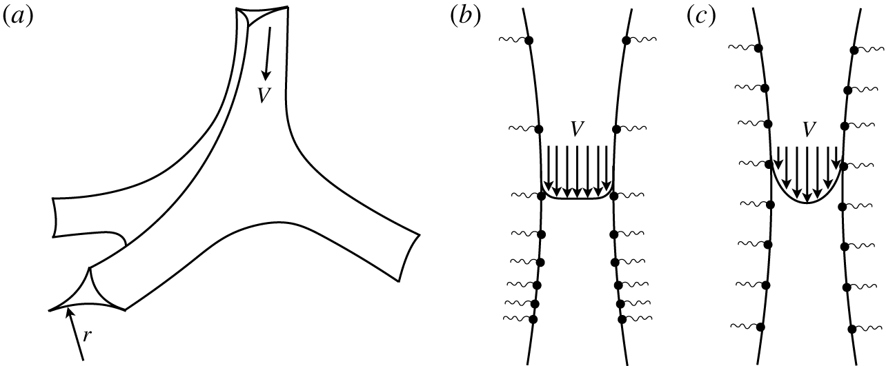
Figure 22. (a) Geometry of a node at the intersection of four Plateau borders. (b) Flow along a longitudinal section of a channel is plug-like when $Bq\ll 1$
. Viscous dissipation occurs primarily at the nodes (not shown) in this case. (c) Poiseuille flow for
$Bq\ll 1$
. Viscous dissipation occurs primarily at the nodes (not shown) in this case. (c) Poiseuille flow for $Bq\gg 1$
, corresponding to large interfacial stresses and subsequent surface immobilization.
$Bq\gg 1$
, corresponding to large interfacial stresses and subsequent surface immobilization.
4.5.1 Physico-chemical model
We simplify the geometry by considering only a planar projection of a vertical liquid channel (figure 22) of width $2h(z)$
. The non-trivial shape of the channel and its orientation relative to gravity will modify the following analysis, but only by numerical prefactors (Koehler et al.
Reference Koehler, Hilgenfeldt and Stone2000; Durand & Langevin Reference Durand and Langevin2002). As with coating flows, we exploit the fact that
$2h(z)$
. The non-trivial shape of the channel and its orientation relative to gravity will modify the following analysis, but only by numerical prefactors (Koehler et al.
Reference Koehler, Hilgenfeldt and Stone2000; Durand & Langevin Reference Durand and Langevin2002). As with coating flows, we exploit the fact that $r\ll L$
, and use lubrication theory for the bulk fluid flow:
$r\ll L$
, and use lubrication theory for the bulk fluid flow:
 $$\begin{eqnarray}\unicode[STIX]{x1D702}\frac{\unicode[STIX]{x2202}^{2}u}{\unicode[STIX]{x2202}x^{2}}=\frac{\unicode[STIX]{x2202}P}{\unicode[STIX]{x2202}z},\end{eqnarray}$$
where $P(z)=p(z)-\unicode[STIX]{x1D70C}gz$
. Integrating (4.121) and imposing boundary conditions
$P(z)=p(z)-\unicode[STIX]{x1D70C}gz$
. Integrating (4.121) and imposing boundary conditions $u(x=\pm h)=u_{s}$
gives
$u(x=\pm h)=u_{s}$
gives
 $$\begin{eqnarray}u(x,z)=\frac{x^{2}-h^{2}}{2\unicode[STIX]{x1D702}}\frac{\unicode[STIX]{x2202}P}{\unicode[STIX]{x2202}z}+u_{s},\end{eqnarray}$$
where the surface velocity $u_{s}$
is yet unknown and will be determined by the surface stress balance. The fluid pressure,
$u_{s}$
is yet unknown and will be determined by the surface stress balance. The fluid pressure, $p$
, relative to the gas pressure in the bubbles obeys the Young–Laplace equation, giving
$p$
, relative to the gas pressure in the bubbles obeys the Young–Laplace equation, giving
 $$\begin{eqnarray}\frac{\unicode[STIX]{x2202}P}{\unicode[STIX]{x2202}z}\approx \frac{\unicode[STIX]{x1D6FE}}{h^{2}}\frac{\unicode[STIX]{x2202}h}{\unicode[STIX]{x2202}z}-\unicode[STIX]{x1D70C}g,\end{eqnarray}$$
where the total curvature is assumed to be $1/h(z)$
.
$1/h(z)$
.
Conservation of mass within the channel requires
 $$\begin{eqnarray}\frac{\unicode[STIX]{x2202}h}{\unicode[STIX]{x2202}t}+\frac{\unicode[STIX]{x2202}}{\unicode[STIX]{x2202}z}\left[\int _{-h}^{h}u(x,z)\,\text{d}x\right]=0,\end{eqnarray}$$
and substituting $u(x,z)$
from (4.122) gives the drainage equation for each channel
$u(x,z)$
from (4.122) gives the drainage equation for each channel
 $$\begin{eqnarray}\frac{\unicode[STIX]{x2202}h}{\unicode[STIX]{x2202}t}+\frac{\unicode[STIX]{x2202}}{\unicode[STIX]{x2202}z}\left[-\frac{h^{3}}{3\unicode[STIX]{x1D702}}\frac{\unicode[STIX]{x2202}P}{\unicode[STIX]{x2202}z}+2u_{s}h\right]=0.\end{eqnarray}$$
The surface velocity $u_{s}$
in (4.125) is dictated by the interfacial stress balance (3.94)
$u_{s}$
in (4.125) is dictated by the interfacial stress balance (3.94)
 $$\begin{eqnarray}-\frac{E_{0}}{\unicode[STIX]{x1D6E4}_{0}}\frac{\unicode[STIX]{x2202}\unicode[STIX]{x1D6E4}}{\unicode[STIX]{x2202}z}+(\unicode[STIX]{x1D702}_{s}+\unicode[STIX]{x1D705}_{s})\frac{\unicode[STIX]{x2202}^{2}u_{s}}{\unicode[STIX]{x2202}z^{2}}=h\frac{\unicode[STIX]{x2202}P}{\unicode[STIX]{x2202}z}.\end{eqnarray}$$
Reverse Marangoni stresses are driven by gradients in $\unicode[STIX]{x1D6E4}$
, as described by the balance between surface convection and diffusion, or adsorption/desorption, as pursued in previous sections.
$\unicode[STIX]{x1D6E4}$
, as described by the balance between surface convection and diffusion, or adsorption/desorption, as pursued in previous sections.
We will choose one illustrative case that is analytically tractable. If the surfactant is surface inviscid ( $\unicode[STIX]{x1D702}_{s}=0$
,
$\unicode[STIX]{x1D702}_{s}=0$
, $\unicode[STIX]{x1D705}_{s}=0$
) and insoluble (
$\unicode[STIX]{x1D705}_{s}=0$
) and insoluble ( $\unicode[STIX]{x1D70F}_{s}^{-1}=0$
), gradients in
$\unicode[STIX]{x1D70F}_{s}^{-1}=0$
), gradients in $\unicode[STIX]{x1D6E4}$
can only relax via surface diffusion. Durand & Langevin (Reference Durand and Langevin2002) solved the surfactant conservation equation for
$\unicode[STIX]{x1D6E4}$
can only relax via surface diffusion. Durand & Langevin (Reference Durand and Langevin2002) solved the surfactant conservation equation for $\unicode[STIX]{x1D6E4}$
, using (4.126) to obtain
$\unicode[STIX]{x1D6E4}$
, using (4.126) to obtain
 $$\begin{eqnarray}u_{s}=-\frac{D_{s}}{E_{0}}h\frac{\unicode[STIX]{x2202}P}{\unicode[STIX]{x2202}z},\end{eqnarray}$$
which when substituted in (4.125) along with (4.123) gives the drainage equation
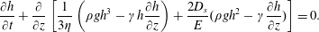 $$\begin{eqnarray}\frac{\unicode[STIX]{x2202}h}{\unicode[STIX]{x2202}t}+\frac{\unicode[STIX]{x2202}}{\unicode[STIX]{x2202}z}\left[\frac{1}{3\unicode[STIX]{x1D702}}\left(\unicode[STIX]{x1D70C}gh^{3}-\unicode[STIX]{x1D6FE}h\frac{\unicode[STIX]{x2202}h}{\unicode[STIX]{x2202}z}\right)+\frac{2D_{s}}{E}(\unicode[STIX]{x1D70C}gh^{2}-\unicode[STIX]{x1D6FE}\frac{\unicode[STIX]{x2202}h}{\unicode[STIX]{x2202}z})\right]=0.\end{eqnarray}$$
Analogous drainage equations can be derived for more general 3-D networks and written in terms of the cross-sectional area $A\propto h^{2}$
of the channel. A measurable quantity is the volume fraction
$A\propto h^{2}$
of the channel. A measurable quantity is the volume fraction $\unicode[STIX]{x1D716}(z,t)$
of liquid in the foam, which relates to the channel cross-sectional area
$\unicode[STIX]{x1D716}(z,t)$
of liquid in the foam, which relates to the channel cross-sectional area $A(z,t)$
via
$A(z,t)$
via $\unicode[STIX]{x1D716}\sim (AL)/L^{3}$
. A generalized 3-D foam drainage equation emerges,
$\unicode[STIX]{x1D716}\sim (AL)/L^{3}$
. A generalized 3-D foam drainage equation emerges,
 $$\begin{eqnarray}\frac{\unicode[STIX]{x2202}\unicode[STIX]{x1D716}}{\unicode[STIX]{x2202}t}+\frac{\unicode[STIX]{x2202}}{\unicode[STIX]{x2202}z}\left[\unicode[STIX]{x1D6FF}_{1}\frac{L^{2}}{\unicode[STIX]{x1D702}}\left(\unicode[STIX]{x1D70C}g\unicode[STIX]{x1D716}^{2}-\unicode[STIX]{x1D6FF}_{0}\frac{\unicode[STIX]{x1D6FE}}{L}\frac{\unicode[STIX]{x2202}\unicode[STIX]{x1D716}^{3/2}}{\unicode[STIX]{x2202}z}\right)+\unicode[STIX]{x1D6FF}_{2}\frac{D_{s}L}{E_{0}}\left(\unicode[STIX]{x1D70C}g\unicode[STIX]{x1D716}^{3/2}-\unicode[STIX]{x1D6FF}_{0}\frac{\unicode[STIX]{x1D6FE}}{L}\frac{\unicode[STIX]{x2202}\unicode[STIX]{x1D716}}{\unicode[STIX]{x2202}z}\right)\right]=0,\end{eqnarray}$$
where $\unicode[STIX]{x1D6FF}_{0}$
,
$\unicode[STIX]{x1D6FF}_{0}$
, $\unicode[STIX]{x1D6FF}_{1}$
and
$\unicode[STIX]{x1D6FF}_{1}$
and $\unicode[STIX]{x1D6FF}_{2}$
are numerical constants that depend on the particular geometry of the Plateau borders (Koehler et al.
Reference Koehler, Hilgenfeldt and Stone2000; Durand & Langevin Reference Durand and Langevin2002). Non-dimensionalizing length and time in (4.129) over
$\unicode[STIX]{x1D6FF}_{2}$
are numerical constants that depend on the particular geometry of the Plateau borders (Koehler et al.
Reference Koehler, Hilgenfeldt and Stone2000; Durand & Langevin Reference Durand and Langevin2002). Non-dimensionalizing length and time in (4.129) over $\unicode[STIX]{x1D6FF}_{0}\unicode[STIX]{x1D6FE}/\unicode[STIX]{x1D70C}gL$
and
$\unicode[STIX]{x1D6FF}_{0}\unicode[STIX]{x1D6FE}/\unicode[STIX]{x1D70C}gL$
and $\unicode[STIX]{x1D6FF}_{0}\unicode[STIX]{x1D6FE}\unicode[STIX]{x1D702}/\unicode[STIX]{x1D6FF}_{1}\unicode[STIX]{x1D70C}^{2}g^{2}L^{3}$
gives
$\unicode[STIX]{x1D6FF}_{0}\unicode[STIX]{x1D6FE}\unicode[STIX]{x1D702}/\unicode[STIX]{x1D6FF}_{1}\unicode[STIX]{x1D70C}^{2}g^{2}L^{3}$
gives
 $$\begin{eqnarray}\frac{\unicode[STIX]{x2202}\unicode[STIX]{x1D716}}{\unicode[STIX]{x2202}\tilde{t}}+\frac{\unicode[STIX]{x2202}}{\unicode[STIX]{x2202}\tilde{z}}\left[\unicode[STIX]{x1D716}^{2}-\frac{\unicode[STIX]{x2202}\unicode[STIX]{x1D716}^{3/2}}{\unicode[STIX]{x2202}\tilde{z}}+\frac{\unicode[STIX]{x1D6FF}_{2}}{\unicode[STIX]{x1D6FF}_{1}Ma_{D}}\left(\unicode[STIX]{x1D716}^{3/2}-\frac{\unicode[STIX]{x2202}\unicode[STIX]{x1D716}}{\unicode[STIX]{x2202}\tilde{z}}\right)\right]=0,\end{eqnarray}$$
where the surface diffusive Marangoni number is $Ma_{D}=E_{0}L/\unicode[STIX]{x1D702}D_{s}$
, as in table 3.
$Ma_{D}=E_{0}L/\unicode[STIX]{x1D702}D_{s}$
, as in table 3.
Marangoni reverse flows are strongest when surface diffusion is weak, and $Ma_{D}\gg 1$
, in which case (4.130) becomes
$Ma_{D}\gg 1$
, in which case (4.130) becomes
 $$\begin{eqnarray}\frac{\unicode[STIX]{x2202}\unicode[STIX]{x1D716}}{\unicode[STIX]{x2202}\tilde{t}}+\frac{\unicode[STIX]{x2202}\unicode[STIX]{x1D716}^{2}}{\unicode[STIX]{x2202}\tilde{z}}-\frac{\unicode[STIX]{x2202}^{2}\unicode[STIX]{x1D716}^{3/2}}{\unicode[STIX]{x2202}\tilde{z}^{2}}=0.\end{eqnarray}$$
In this rigid-interface limit, the channels are essentially no-slip walls, and bulk fluid flow within the channels is Poiseuille-like. This model was first given by Verbist et al. (Reference Verbist, Weaire and Kraynik1996), who derived it from a macroscopic perspective as we illustrate in the next section. The dominant resistance to foam drainage in the rigid-interface limit arises from bulk viscous dissipation.
By contrast, strong surface diffusion quickly eliminates surface concentration gradients when $Ma_{D}\ll 1$
, thereby weakening Marangoni reverse flows. Rescaling the characteristic time in (4.130) by
$Ma_{D}\ll 1$
, thereby weakening Marangoni reverse flows. Rescaling the characteristic time in (4.130) by $\unicode[STIX]{x1D6FF}_{1}Ma_{D}/\unicode[STIX]{x1D6FF}_{2}$
in this limit gives
$\unicode[STIX]{x1D6FF}_{1}Ma_{D}/\unicode[STIX]{x1D6FF}_{2}$
in this limit gives
 $$\begin{eqnarray}\frac{\unicode[STIX]{x2202}\unicode[STIX]{x1D716}}{\unicode[STIX]{x2202}\tilde{t}}+\frac{\unicode[STIX]{x2202}\unicode[STIX]{x1D716}^{3/2}}{\unicode[STIX]{x2202}\tilde{z}}-\frac{\unicode[STIX]{x2202}^{2}\unicode[STIX]{x1D716}}{\unicode[STIX]{x2202}\tilde{z}^{2}}=0.\end{eqnarray}$$
This mobile-interface drainage equation represents channels with plug-like bulk flow: the surface is completely stress free or ‘remobilized’ in this limit. The resistance to fluid flow arises from dissipation at the channel surfaces. In the following sections, we will explore the measurable macroscopic signatures of these two limits.
4.5.2 Macroscopic model
The analysis thus far ignored the nodes that connect Plateau borders within the foam network. Mixing, merging and bending of streamlines at nodes occur over length scales $r\ll L$
, and therefore increase viscous dissipation. The detailed flow in the nodes (Cohen-Addad et al.
Reference Cohen-Addad, Höhler and Pitois2013) is beyond the scope of our discussion, and we will instead outline a course-grained model (Koehler et al.
Reference Koehler, Hilgenfeldt and Stone2000) that treats the foam as a porous macroscopic material.
$r\ll L$
, and therefore increase viscous dissipation. The detailed flow in the nodes (Cohen-Addad et al.
Reference Cohen-Addad, Höhler and Pitois2013) is beyond the scope of our discussion, and we will instead outline a course-grained model (Koehler et al.
Reference Koehler, Hilgenfeldt and Stone2000) that treats the foam as a porous macroscopic material.
Mass conservation in the foam network requires
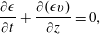 $$\begin{eqnarray}\frac{\unicode[STIX]{x2202}\unicode[STIX]{x1D716}}{\unicode[STIX]{x2202}t}+\frac{\unicode[STIX]{x2202}(\unicode[STIX]{x1D716}v)}{\unicode[STIX]{x2202}z}=0,\end{eqnarray}$$
where the mean velocity $v$
obeys Darcy’s law
$v$
obeys Darcy’s law
 $$\begin{eqnarray}\frac{\unicode[STIX]{x2202}P}{\unicode[STIX]{x2202}z}+\frac{\unicode[STIX]{x1D702}v}{k(\unicode[STIX]{x1D716})}=0.\end{eqnarray}$$
All details of the network and dissipation within the foam are lumped into a permeability $k(\unicode[STIX]{x1D716})$
in (4.134). The foam is driven by both capillary and hydrostatic pressures
$k(\unicode[STIX]{x1D716})$
in (4.134). The foam is driven by both capillary and hydrostatic pressures
 $$\begin{eqnarray}P(z)=p_{gas}-\frac{\unicode[STIX]{x1D6FE}}{r}-\unicode[STIX]{x1D70C}gz\approx p_{gas}-\frac{\unicode[STIX]{x1D6FE}\unicode[STIX]{x1D6FF}_{\unicode[STIX]{x1D716}}^{1/2}}{L\unicode[STIX]{x1D716}^{1/2}}-\unicode[STIX]{x1D70C}gz,\end{eqnarray}$$
where the radius of curvature is assumed to be small ( $r\ll L$
), and the foam is assumed to be dry (
$r\ll L$
), and the foam is assumed to be dry ( $\unicode[STIX]{x1D716}\ll 1$
) so that
$\unicode[STIX]{x1D716}\ll 1$
) so that $r\approx \unicode[STIX]{x1D6FF}_{\unicode[STIX]{x1D716}}^{-1/2}L\unicode[STIX]{x1D716}^{1/2}$
from (4.120). Using (4.135) in (4.134) gives
$r\approx \unicode[STIX]{x1D6FF}_{\unicode[STIX]{x1D716}}^{-1/2}L\unicode[STIX]{x1D716}^{1/2}$
from (4.120). Using (4.135) in (4.134) gives
 $$\begin{eqnarray}\unicode[STIX]{x1D70C}g+\frac{\unicode[STIX]{x1D6FE}\unicode[STIX]{x1D6FF}_{\unicode[STIX]{x1D716}}^{1/2}}{L}\frac{\unicode[STIX]{x2202}\unicode[STIX]{x1D716}^{-1/2}}{\unicode[STIX]{x2202}z}=\frac{\unicode[STIX]{x1D702}v}{k(\unicode[STIX]{x1D716})},\end{eqnarray}$$
which can be solved for $v$
in terms of the permeability
$v$
in terms of the permeability $k(\unicode[STIX]{x1D716})$
. Mass conservation (4.133) then becomes
$k(\unicode[STIX]{x1D716})$
. Mass conservation (4.133) then becomes
 $$\begin{eqnarray}\frac{\unicode[STIX]{x2202}\unicode[STIX]{x1D716}}{\unicode[STIX]{x2202}t}+\frac{\unicode[STIX]{x2202}}{\unicode[STIX]{x2202}z}\left[\frac{\unicode[STIX]{x1D70C}g}{\unicode[STIX]{x1D702}}k(\unicode[STIX]{x1D716})\unicode[STIX]{x1D716}-\frac{\unicode[STIX]{x1D6FE}\unicode[STIX]{x1D6FF}_{\unicode[STIX]{x1D716}}^{1/2}}{\unicode[STIX]{x1D702}L}k(\unicode[STIX]{x1D716})\frac{\unicode[STIX]{x2202}\unicode[STIX]{x1D716}^{1/2}}{\unicode[STIX]{x2202}z}\right]=0,\end{eqnarray}$$
which is the generalized macroscopic foam drainage model.
The permeability $k(\unicode[STIX]{x1D716})$
, in general, depends on the geometry and boundary conditions for the flow within the foam network (Koehler et al.
Reference Koehler, Hilgenfeldt and Stone2000). When Marangoni and/or surface-viscous effects immobilize the interface, bulk flow within the channels is Poiseuille-like. The permeability
$k(\unicode[STIX]{x1D716})$
, in general, depends on the geometry and boundary conditions for the flow within the foam network (Koehler et al.
Reference Koehler, Hilgenfeldt and Stone2000). When Marangoni and/or surface-viscous effects immobilize the interface, bulk flow within the channels is Poiseuille-like. The permeability $k(\unicode[STIX]{x1D716})$
then comes from balancing the fluid pressure gradient
$k(\unicode[STIX]{x1D716})$
then comes from balancing the fluid pressure gradient $\unicode[STIX]{x1D702}V/r^{2}$
with that driving the Darcy flow
$\unicode[STIX]{x1D702}V/r^{2}$
with that driving the Darcy flow $\unicode[STIX]{x1D702}V/k(\unicode[STIX]{x1D716})$
, implying
$\unicode[STIX]{x1D702}V/k(\unicode[STIX]{x1D716})$
, implying
 $$\begin{eqnarray}k(\unicode[STIX]{x1D716})\propto r^{2}\propto L^{2}\unicode[STIX]{x1D716}.\end{eqnarray}$$
Using $k(\unicode[STIX]{x1D716})\sim L^{2}\unicode[STIX]{x1D716}$
in (4.137) gives the (dimensional) rigid-interface drainage equation, (4.131).
$k(\unicode[STIX]{x1D716})\sim L^{2}\unicode[STIX]{x1D716}$
in (4.137) gives the (dimensional) rigid-interface drainage equation, (4.131).
By contrast, if surface stresses are negligible and interfaces are mobile, flow in the channels is plug-like. The dominant viscous resistance then comes from the merging flows at nodes, which occupy a fraction of $O(r/L)$
of the total fluid volume. When the resistance to Darcy flow,
$O(r/L)$
of the total fluid volume. When the resistance to Darcy flow, $\unicode[STIX]{x1D702}V/k(\unicode[STIX]{x1D716})$
, arises from the volume-averaged viscous resistance at nodes,
$\unicode[STIX]{x1D702}V/k(\unicode[STIX]{x1D716})$
, arises from the volume-averaged viscous resistance at nodes, $(\unicode[STIX]{x1D702}V/r^{2})(r/L)$
, the foam permeability becomes
$(\unicode[STIX]{x1D702}V/r^{2})(r/L)$
, the foam permeability becomes
 $$\begin{eqnarray}k(\unicode[STIX]{x1D716})\propto rL\propto L^{2}\unicode[STIX]{x1D716}^{1/2}.\end{eqnarray}$$
Substituting $k(\unicode[STIX]{x1D716})\sim L^{2}\unicode[STIX]{x1D716}^{1/2}$
in (4.137) gives the node-dominated foam drainage equation (Koehler et al.
Reference Koehler, Hilgenfeldt and Stone2000), which is identical to the mobile-interface drainage equation (4.132). However, the resistance to fluid drainage in this limit arises due to bulk viscous dissipation at the nodes, rather than surface stresses. In other words, flow in channels can be plug-like even when channel-dominated if the driving pressure gradient balances surface stresses via (4.126).
$k(\unicode[STIX]{x1D716})\sim L^{2}\unicode[STIX]{x1D716}^{1/2}$
in (4.137) gives the node-dominated foam drainage equation (Koehler et al.
Reference Koehler, Hilgenfeldt and Stone2000), which is identical to the mobile-interface drainage equation (4.132). However, the resistance to fluid drainage in this limit arises due to bulk viscous dissipation at the nodes, rather than surface stresses. In other words, flow in channels can be plug-like even when channel-dominated if the driving pressure gradient balances surface stresses via (4.126).
More generally, we expect surfactant processes to impact flow in foams via a lumped immobilization parameter
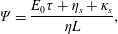 $$\begin{eqnarray}\unicode[STIX]{x1D6F9}=\frac{E_{0}\unicode[STIX]{x1D70F}+\unicode[STIX]{x1D702}_{s}+\unicode[STIX]{x1D705}_{s}}{\unicode[STIX]{x1D702}L},\end{eqnarray}$$
where $\unicode[STIX]{x1D70F}$
is the time scale of the dominant surfactant process that relaxes Marangoni stresses. If the channel walls are not immobilized, the surface ‘slips’ as the foam drains. Surface stresses associated with such a deformation scale like
$\unicode[STIX]{x1D70F}$
is the time scale of the dominant surfactant process that relaxes Marangoni stresses. If the channel walls are not immobilized, the surface ‘slips’ as the foam drains. Surface stresses associated with such a deformation scale like $(E_{0}\unicode[STIX]{x1D70F}+\unicode[STIX]{x1D702}_{s}+\unicode[STIX]{x1D705}_{s})V/L^{2}$
, which translates to a force per unit volume of the fluid of
$(E_{0}\unicode[STIX]{x1D70F}+\unicode[STIX]{x1D702}_{s}+\unicode[STIX]{x1D705}_{s})V/L^{2}$
, which translates to a force per unit volume of the fluid of $(E_{0}\unicode[STIX]{x1D70F}+\unicode[STIX]{x1D702}_{s}+\unicode[STIX]{x1D705}_{s})V/rL^{2}$
. Equating this force to the macroscopic driving force density
$(E_{0}\unicode[STIX]{x1D70F}+\unicode[STIX]{x1D702}_{s}+\unicode[STIX]{x1D705}_{s})V/rL^{2}$
. Equating this force to the macroscopic driving force density $\unicode[STIX]{x1D702}V/k(\unicode[STIX]{x1D716})$
gives permeability
$\unicode[STIX]{x1D702}V/k(\unicode[STIX]{x1D716})$
gives permeability
 $$\begin{eqnarray}k(\unicode[STIX]{x1D716},\unicode[STIX]{x1D6F9})\propto \frac{\unicode[STIX]{x1D702}L^{2}r}{E\unicode[STIX]{x1D70F}+\unicode[STIX]{x1D702}_{s}+\unicode[STIX]{x1D705}_{s}}\propto \frac{L^{2}\unicode[STIX]{x1D716}^{1/2}}{\unicode[STIX]{x1D6F9}}.\end{eqnarray}$$
The permeability of channels increases with decreasing degree of immobilization: a ‘slippier’ interface makes flow more plug-like. Substituting $k(\unicode[STIX]{x1D716})\sim L^{2}\unicode[STIX]{x1D716}^{1/2}/\unicode[STIX]{x1D6F9}$
in (4.137) and setting
$k(\unicode[STIX]{x1D716})\sim L^{2}\unicode[STIX]{x1D716}^{1/2}/\unicode[STIX]{x1D6F9}$
in (4.137) and setting $\unicode[STIX]{x1D6F9}=Ma_{D}$
gives the dimensional analogue of the mobile-interface drainage equation (4.132).
$\unicode[STIX]{x1D6F9}=Ma_{D}$
gives the dimensional analogue of the mobile-interface drainage equation (4.132).
4.5.3 Foam drainage: predictions versus observations
Forced foam drainage experiments introduce fluid from the top at flow rate $Q$
into a dry foam, and track the velocity
$Q$
into a dry foam, and track the velocity $v$
of a wet front as it moves downwards through the foam. The front moves at a velocity
$v$
of a wet front as it moves downwards through the foam. The front moves at a velocity
 $$\begin{eqnarray}v\propto Q^{\unicode[STIX]{x1D6FC}},\end{eqnarray}$$
where the exponent $\unicode[STIX]{x1D6FC}$
is typically between
$\unicode[STIX]{x1D6FC}$
is typically between $1/3$
and
$1/3$
and $1/2$
(Verbist et al.
Reference Verbist, Weaire and Kraynik1996; Koehler et al.
Reference Koehler, Hilgenfeldt and Stone2000; Durand & Langevin Reference Durand and Langevin2002). Surfactant processes impact this exponent in a measurable way.
$1/2$
(Verbist et al.
Reference Verbist, Weaire and Kraynik1996; Koehler et al.
Reference Koehler, Hilgenfeldt and Stone2000; Durand & Langevin Reference Durand and Langevin2002). Surfactant processes impact this exponent in a measurable way.
The drainage equation in both channel- and node-dominated limits can be solved by modelling the wetted front as a soliton wave
 $$\begin{eqnarray}\unicode[STIX]{x1D716}(z,t)=f(s)=f(z-vt),\end{eqnarray}$$
which travels downward at a constant front velocity $v$
. The foam is assumed to be dry far ahead of the moving front, and uniformly wetted far behind the front
$v$
. The foam is assumed to be dry far ahead of the moving front, and uniformly wetted far behind the front
 $$\begin{eqnarray}f(s\rightarrow \infty )=0,\quad \text{and}\quad f^{\prime }(s\rightarrow -\infty )=0.\end{eqnarray}$$
Verbist et al. (Reference Verbist, Weaire and Kraynik1996) and Koehler et al. (Reference Koehler, Hilgenfeldt and Stone2000) describe this solution in detail for (4.131) and (4.132), respectively. Fortunately, the exponent $\unicode[STIX]{x1D6FC}$
can be deduced without solving for the front profile. In the channel-dominated or rigid-interface limit, transforming (4.131) using
$\unicode[STIX]{x1D6FC}$
can be deduced without solving for the front profile. In the channel-dominated or rigid-interface limit, transforming (4.131) using $s=z-vt$
, and integrating once gives
$s=z-vt$
, and integrating once gives
 $$\begin{eqnarray}-vf+f^{2}-(f^{3/2})^{\prime }=0.\end{eqnarray}$$
Using the $s\rightarrow -\infty$
condition (4.144) in (4.145) then gives
$s\rightarrow -\infty$
condition (4.144) in (4.145) then gives
 $$\begin{eqnarray}f(s\rightarrow -\infty )=\unicode[STIX]{x1D716}(z\rightarrow -\infty )\rightarrow v.\end{eqnarray}$$
For a foam of cross-section area $A$
, a macroscopic volume
$A$
, a macroscopic volume $vA\unicode[STIX]{x0394}t$
is wetted behind the moving front by a volume
$vA\unicode[STIX]{x0394}t$
is wetted behind the moving front by a volume $Q\unicode[STIX]{x0394}t$
of fluid supplied at the top. The wetted volume fraction is then
$Q\unicode[STIX]{x0394}t$
of fluid supplied at the top. The wetted volume fraction is then
 $$\begin{eqnarray}\unicode[STIX]{x1D716}=\frac{Q}{vA}.\end{eqnarray}$$
For the wetted region far behind the front, (4.146) gives
 $$\begin{eqnarray}\frac{Q}{vA}\rightarrow v\quad \Rightarrow \quad v\propto Q^{1/2},\quad \text{i.e.}\quad \unicode[STIX]{x1D6FC}=1/2.\end{eqnarray}$$
This scaling would be expected in a foam drainage experiment when the channel surfaces are immobilized, and the foam is essentially a network of connected tubes with Poiseuille flow through each channel.
By contrast, transforming and integrating (4.132) for the mobile-interface or node-dominated regime gives
 $$\begin{eqnarray}-vf+f^{3/2}-f^{\prime }=0.\end{eqnarray}$$
The boundary condition as $s\rightarrow -\infty$
(4.144) gives
$s\rightarrow -\infty$
(4.144) gives
 $$\begin{eqnarray}f(s\rightarrow -\infty )=\unicode[STIX]{x1D716}(z\rightarrow -\infty )\rightarrow v^{2}.\end{eqnarray}$$
Then, in the wetted region far behind the moving front,
 $$\begin{eqnarray}\unicode[STIX]{x1D716}=\frac{Q}{vA}\rightarrow v^{2}\quad \Rightarrow \quad v\propto Q^{1/3},\quad \text{i.e.}\quad \unicode[STIX]{x1D6FC}=1/3.\end{eqnarray}$$
The transition from Poiseuille-like flow in immobilized channels to plug-like flow in mobile channels manifests as a change in the exponent $\unicode[STIX]{x1D6FC}$
in (4.142) from
$\unicode[STIX]{x1D6FC}$
in (4.142) from $1/2$
to
$1/2$
to $1/3$
.
$1/3$
.
Surfactants change the character of drainage based on the extent of surface immobilization. Durand, Martinoty & Langevin (Reference Durand, Martinoty and Langevin1999) measured the exponent $\unicode[STIX]{x1D6FC}$
to transition between the two types of flow upon modifying surface rheology. The foam literature historically quantifies this transition in terms of the ‘Kraynik criterion’ (Koehler et al.
Reference Koehler, Hilgenfeldt and Stone2000; Durand & Langevin Reference Durand and Langevin2002) based on the surface shear viscosity
$\unicode[STIX]{x1D6FC}$
to transition between the two types of flow upon modifying surface rheology. The foam literature historically quantifies this transition in terms of the ‘Kraynik criterion’ (Koehler et al.
Reference Koehler, Hilgenfeldt and Stone2000; Durand & Langevin Reference Durand and Langevin2002) based on the surface shear viscosity
 $$\begin{eqnarray}M_{K}=\frac{r\unicode[STIX]{x1D702}}{\unicode[STIX]{x1D702}_{s}}=\frac{1}{Bq}.\end{eqnarray}$$
Large $M_{K}$
(or small
$M_{K}$
(or small $Bq$
) corresponds to mobile channel surfaces, and small
$Bq$
) corresponds to mobile channel surfaces, and small $M_{K}$
(or large
$M_{K}$
(or large $Bq$
) justifies the assumption of rigid channel walls.
$Bq$
) justifies the assumption of rigid channel walls.
However, $\unicode[STIX]{x1D702}_{s}$
,
$\unicode[STIX]{x1D702}_{s}$
, $\unicode[STIX]{x1D705}_{s}$
and
$\unicode[STIX]{x1D705}_{s}$
and $E_{0}\unicode[STIX]{x1D70F}_{s}$
play indistinguishable roles in 1-D compression/dilatation of interfaces, as noted in § 3.4.3. What was previously attributed to dissipation due to a surface shear viscosity might arise from an intrinsic surface dilatational viscosity, or due to Marangoni stresses with finite-time adsorption/desorption, or some combination (Buzza et al.
Reference Buzza, Lu and Cates1995). More generally, therefore, the transition from one drainage regime to the other should depend on the degree of immobilization
$E_{0}\unicode[STIX]{x1D70F}_{s}$
play indistinguishable roles in 1-D compression/dilatation of interfaces, as noted in § 3.4.3. What was previously attributed to dissipation due to a surface shear viscosity might arise from an intrinsic surface dilatational viscosity, or due to Marangoni stresses with finite-time adsorption/desorption, or some combination (Buzza et al.
Reference Buzza, Lu and Cates1995). More generally, therefore, the transition from one drainage regime to the other should depend on the degree of immobilization $\unicode[STIX]{x1D6F9}$
. When
$\unicode[STIX]{x1D6F9}$
. When $\unicode[STIX]{x1D6F9}\gg 1$
, the surface is immobilized, flow within the channels is Poiseuille-like, and the drainage exponent
$\unicode[STIX]{x1D6F9}\gg 1$
, the surface is immobilized, flow within the channels is Poiseuille-like, and the drainage exponent $\unicode[STIX]{x1D6FC}$
is closer to
$\unicode[STIX]{x1D6FC}$
is closer to $1/2$
. By contrast, channel surfaces are mobile when
$1/2$
. By contrast, channel surfaces are mobile when $\unicode[STIX]{x1D6F9}\ll 1$
, flow within the Plateau borders are plug-like, and
$\unicode[STIX]{x1D6F9}\ll 1$
, flow within the Plateau borders are plug-like, and $\unicode[STIX]{x1D6FC}\approx 1/3$
.
$\unicode[STIX]{x1D6FC}\approx 1/3$
.
4.6 Particles and probes on surfactant-laden interfaces
Early descriptions of particle motion within viscous interfaces were motivated by the dynamics of membrane-bound proteins. Saffman & Delbrück (Reference Saffman and Delbrück1975) approximated the phospholipid membrane as a thin fluid layer of thickness $h$
and 3-D viscosity
$h$
and 3-D viscosity $\unicode[STIX]{x1D702}_{m}$
atop a subphase of viscosity
$\unicode[STIX]{x1D702}_{m}$
atop a subphase of viscosity $\unicode[STIX]{x1D702}$
(figure 12). A modern interpretation of this system would introduce a surface shear viscosity
$\unicode[STIX]{x1D702}$
(figure 12). A modern interpretation of this system would introduce a surface shear viscosity $\unicode[STIX]{x1D702}_{s}=\unicode[STIX]{x1D702}_{m}h$
. Saffman (Reference Saffman1976) solved this problem asymptotically in the interface-dominated (
$\unicode[STIX]{x1D702}_{s}=\unicode[STIX]{x1D702}_{m}h$
. Saffman (Reference Saffman1976) solved this problem asymptotically in the interface-dominated ( $Bq\gg 1$
) limit. The leading-order 2-D problem has no steady solution for the translation of a cylinder – the well-known Stokes paradox. This far-field singularity must be regularized by some additional force – Saffman & Delbrück (Reference Saffman and Delbrück1975) examined fluid inertia, finite system size and viscous coupling with subphase liquid. Saffman (Reference Saffman1976), and later Hughes, Pailthorpe & White (Reference Hughes, Pailthorpe and White1981), showed that subphase viscous resistance resolves the paradox in many practical systems. In addition to predicting membrane protein diffusivity, these relations help deduce surface rheology from the measured mobility of surface-attached probes (Prasad et al.
Reference Prasad, Koehler and Weeks2006; Fuller & Vermant Reference Fuller and Vermant2012; Zell et al.
Reference Zell, Nowbahar, Mansard, Leal, Deshmukh, Mecca, Tucker and Squires2014), and form the basis for interfacial microrheology.
$Bq\gg 1$
) limit. The leading-order 2-D problem has no steady solution for the translation of a cylinder – the well-known Stokes paradox. This far-field singularity must be regularized by some additional force – Saffman & Delbrück (Reference Saffman and Delbrück1975) examined fluid inertia, finite system size and viscous coupling with subphase liquid. Saffman (Reference Saffman1976), and later Hughes, Pailthorpe & White (Reference Hughes, Pailthorpe and White1981), showed that subphase viscous resistance resolves the paradox in many practical systems. In addition to predicting membrane protein diffusivity, these relations help deduce surface rheology from the measured mobility of surface-attached probes (Prasad et al.
Reference Prasad, Koehler and Weeks2006; Fuller & Vermant Reference Fuller and Vermant2012; Zell et al.
Reference Zell, Nowbahar, Mansard, Leal, Deshmukh, Mecca, Tucker and Squires2014), and form the basis for interfacial microrheology.
4.6.1 Translation and rotation of cylinders
A surface-attached particle translating within an insoluble surfactant monolayer disturbs the surface concentration distribution, potentially setting up reverse Marangoni flows. Assuming weak surfactant diffusivity ( $Ma_{D}\gg 1$
, table 3), these reverse flows modify the fluid streamlines to that of a surface incompressible flow (§ 3.3.2). Using the Green’s function derived in § 3.4.2, the surface velocity field around a moving particle embedded within the monolayer can be written as a boundary integral,
$Ma_{D}\gg 1$
, table 3), these reverse flows modify the fluid streamlines to that of a surface incompressible flow (§ 3.3.2). Using the Green’s function derived in § 3.4.2, the surface velocity field around a moving particle embedded within the monolayer can be written as a boundary integral,
 $$\begin{eqnarray}\boldsymbol{u}_{s}(\boldsymbol{r})=\int _{S}\unicode[STIX]{x1D642}(\boldsymbol{r}-\boldsymbol{r}^{\prime })\boldsymbol{\cdot }\boldsymbol{f}(\boldsymbol{r}^{\prime })\,\text{d}S,\end{eqnarray}$$
where $S$
is the area occupied by the particle, and
$S$
is the area occupied by the particle, and $\boldsymbol{r}^{\prime }\in S$
. The force density
$\boldsymbol{r}^{\prime }\in S$
. The force density $\boldsymbol{f}(\boldsymbol{r}^{\prime })$
is chosen such that
$\boldsymbol{f}(\boldsymbol{r}^{\prime })$
is chosen such that $\boldsymbol{u}_{s}$
satisfies the boundary conditions at the probe surfaces (Fischer Reference Fischer2004b
). The drag force on the particle is then
$\boldsymbol{u}_{s}$
satisfies the boundary conditions at the probe surfaces (Fischer Reference Fischer2004b
). The drag force on the particle is then
 $$\begin{eqnarray}\boldsymbol{F}_{drag}=\int _{S}\boldsymbol{f}(\boldsymbol{r})\,\text{d}S.\end{eqnarray}$$
Alternatively, flow fields can be obtained directly when the system geometry simplifies the Boussinesq–Scriven equations. For example, both the surface velocity $\boldsymbol{u}_{s}$
and bulk velocity
$\boldsymbol{u}_{s}$
and bulk velocity $\boldsymbol{u}$
can be obtained directly for a cylindrical probe (Hughes et al.
Reference Hughes, Pailthorpe and White1981; Barentin et al.
Reference Barentin, Ybert, Di Meglio and Joanny1999) by projecting the governing equations into Fourier–Bessel functions. Then, the drag force can be written as the sum of viscous contributions from the subphase and the monolayer
$\boldsymbol{u}$
can be obtained directly for a cylindrical probe (Hughes et al.
Reference Hughes, Pailthorpe and White1981; Barentin et al.
Reference Barentin, Ybert, Di Meglio and Joanny1999) by projecting the governing equations into Fourier–Bessel functions. Then, the drag force can be written as the sum of viscous contributions from the subphase and the monolayer
 $$\begin{eqnarray}\boldsymbol{F}_{drag}=\int _{S}\hat{\boldsymbol{e}}_{z}\boldsymbol{\cdot }\unicode[STIX]{x1D748}\,\text{d}S+\int _{\unicode[STIX]{x2202}S}\hat{\boldsymbol{e}}_{r}\boldsymbol{\cdot }\unicode[STIX]{x1D748}_{s}\,\text{d}\ell ,\end{eqnarray}$$
where $\unicode[STIX]{x1D748}$
and
$\unicode[STIX]{x1D748}$
and $\unicode[STIX]{x1D748}_{s}$
are stress tensors corresponding to the bulk and the interface, respectively. In the following, we will outline key results from Hughes et al. (Reference Hughes, Pailthorpe and White1981) to illustrate key differences between interface- and bulk-dominated systems.
$\unicode[STIX]{x1D748}_{s}$
are stress tensors corresponding to the bulk and the interface, respectively. In the following, we will outline key results from Hughes et al. (Reference Hughes, Pailthorpe and White1981) to illustrate key differences between interface- and bulk-dominated systems.
The classic Saffman–Delbrück problem consists of a disk of radius $R$
translating or rotating on a planar insoluble interface of surface viscosity
$R$
translating or rotating on a planar insoluble interface of surface viscosity $\unicode[STIX]{x1D702}_{s}$
atop an infinitely deep subphase fluid with viscosity
$\unicode[STIX]{x1D702}_{s}$
atop an infinitely deep subphase fluid with viscosity $\unicode[STIX]{x1D702}$
. The drag
$\unicode[STIX]{x1D702}$
. The drag $\boldsymbol{F}$
against translation at a constant velocity
$\boldsymbol{F}$
against translation at a constant velocity $\boldsymbol{U}$
when the interfacial viscous stresses dominate (
$\boldsymbol{U}$
when the interfacial viscous stresses dominate ( $Bq\gg 1$
) is (Hughes et al.
Reference Hughes, Pailthorpe and White1981)
$Bq\gg 1$
) is (Hughes et al.
Reference Hughes, Pailthorpe and White1981)
 $$\begin{eqnarray}\boldsymbol{F}(Bq\gg 1)=-\frac{4\unicode[STIX]{x03C0}\unicode[STIX]{x1D702}_{s}\boldsymbol{U}}{\ln (2Bq)-\unicode[STIX]{x1D6FE}_{E}+4/(\unicode[STIX]{x03C0}Bq)-\ln (2Bq)/(2Bq^{2})},\end{eqnarray}$$
where $\unicode[STIX]{x1D6FE}_{E}$
is Euler’s constant and the Boussinesq number is
$\unicode[STIX]{x1D6FE}_{E}$
is Euler’s constant and the Boussinesq number is $Bq=\unicode[STIX]{x1D702}_{s}/\unicode[STIX]{x1D702}R=\ell _{SD}/R$
. The Saffman–Delbrück length
$Bq=\unicode[STIX]{x1D702}_{s}/\unicode[STIX]{x1D702}R=\ell _{SD}/R$
. The Saffman–Delbrück length $\ell _{SD}=\unicode[STIX]{x1D702}_{s}/\unicode[STIX]{x1D702}$
(3.102) establishes a ‘cutoff’ beyond which subphase drag dominates over momentum transfer on the interface.
$\ell _{SD}=\unicode[STIX]{x1D702}_{s}/\unicode[STIX]{x1D702}$
(3.102) establishes a ‘cutoff’ beyond which subphase drag dominates over momentum transfer on the interface.
By contrast, when the drag force is dominated by the subphase ( $Bq\ll 1$
), the drag on a disk in an insoluble monolayer is
$Bq\ll 1$
), the drag on a disk in an insoluble monolayer is
 $$\begin{eqnarray}\boldsymbol{F}(Bq\ll 1)=-8\unicode[STIX]{x1D702}R\boldsymbol{U}.\end{eqnarray}$$
This result may at first glance seem surprising, as the drag within an inviscid interface is greater than the drag on a probe translating within a clean interface (Happel & Brenner Reference Happel and Brenner1965),
 $$\begin{eqnarray}\boldsymbol{F}_{clean}=-\frac{16}{3}\unicode[STIX]{x1D702}R\boldsymbol{U}.\end{eqnarray}$$
In other words, the simple addition of a surfactant – even with zero surface viscosity – increases the drag on a disk by a factor of $3/2$
, owing to the effective surface incompressibility boundary condition imposed by the surfactant (§ 3.3.2) in the limit
$3/2$
, owing to the effective surface incompressibility boundary condition imposed by the surfactant (§ 3.3.2) in the limit $Ma\gg 1$
.
$Ma\gg 1$
.
Reverse Marangoni flows modify surface streamlines, which in turn force the bulk fluid to flow in planes parallel to the interface (figure 11). The excess drag in (4.157) arises due to bulk viscous dissipation associated with this modified flow, and not due to surface rheology (Fischer Reference Fischer2004a ). Only drag forces much larger than (4.157) should be attributed to surface rheology.
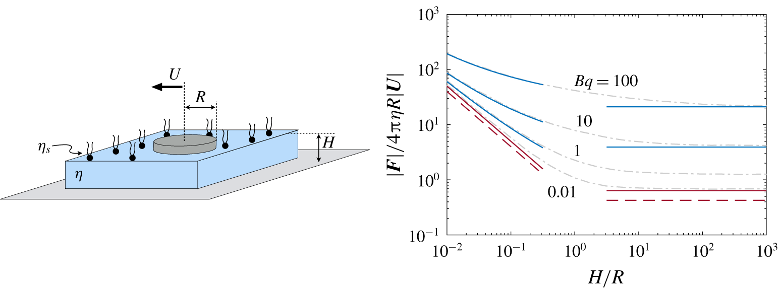
Figure 23. A cylindrical disk translating within an insoluble surfactant monolayer atop a bulk fluid layer of finite depth $H$
. Also shown is the resistance coefficient
$H$
. Also shown is the resistance coefficient $|\boldsymbol{F}|/4\unicode[STIX]{x03C0}\unicode[STIX]{x1D702}R|\boldsymbol{U}|$
as a function of both sublayer thickness and Boussinesq number. The grey dash-dot lines are the numerical calculations of Stone & Ajdari (Reference Stone and Ajdari1998) at specified
$|\boldsymbol{F}|/4\unicode[STIX]{x03C0}\unicode[STIX]{x1D702}R|\boldsymbol{U}|$
as a function of both sublayer thickness and Boussinesq number. The grey dash-dot lines are the numerical calculations of Stone & Ajdari (Reference Stone and Ajdari1998) at specified $Bq$
, and the solid lines are asymptotic values for small and large
$Bq$
, and the solid lines are asymptotic values for small and large $H/R$
. The bottom-most solid lines represent the
$H/R$
. The bottom-most solid lines represent the $Bq\rightarrow 0$
limit (table 4). The dashed asymptotes correspond to a clean interface, from (4.158) and (4.162), and highlights the fact that even an inviscid surfactant increases drag on a translating probe as compared to a surfactant-free surface.
$Bq\rightarrow 0$
limit (table 4). The dashed asymptotes correspond to a clean interface, from (4.158) and (4.162), and highlights the fact that even an inviscid surfactant increases drag on a translating probe as compared to a surfactant-free surface.
The Saffman–Delbrück problem assumes an infinitely deep subphase, and may not be valid for a finite subphase of depth $H$
. The general solution for arbitrary depth obtained numerically by Stone & Ajdari (Reference Stone and Ajdari1998) is shown in figure 23. In the shallow subphase limit (
$H$
. The general solution for arbitrary depth obtained numerically by Stone & Ajdari (Reference Stone and Ajdari1998) is shown in figure 23. In the shallow subphase limit ( $H\ll R$
), Evans & Sackmann (Reference Evans and Sackmann1988) used the lubrication approximation (3.96) to obtain
$H\ll R$
), Evans & Sackmann (Reference Evans and Sackmann1988) used the lubrication approximation (3.96) to obtain
 $$\begin{eqnarray}\boldsymbol{F}(H\ll R)=-\frac{2\unicode[STIX]{x03C0}\unicode[STIX]{x1D702}R^{2}}{H}\frac{\text{K}_{2}(1/Bq_{1})}{\text{K}_{0}(1/Bq_{1})}\boldsymbol{U},\end{eqnarray}$$
where $\text{K}_{n}$
are modified Bessel functions, and
$\text{K}_{n}$
are modified Bessel functions, and $Bq_{1}$
is a Boussinesq number modified to account for finite depth
$Bq_{1}$
is a Boussinesq number modified to account for finite depth
 $$\begin{eqnarray}Bq_{1}^{2}=Bq\frac{H}{R}=\frac{\unicode[STIX]{x1D702}_{s}H}{\unicode[STIX]{x1D702}R^{2}}.\end{eqnarray}$$
When the drag force is dominated by the subphase ( $Bq\ll 1$
), (4.159) gives
$Bq\ll 1$
), (4.159) gives
 $$\begin{eqnarray}\boldsymbol{F}(H\ll R,Bq\rightarrow 0)=-\frac{2\unicode[STIX]{x03C0}\unicode[STIX]{x1D702}R^{2}}{H}\boldsymbol{U}.\end{eqnarray}$$
For comparison, the drag on a probe on a clean interface with a shallow subphase is (Barentin et al. Reference Barentin, Ybert, Di Meglio and Joanny1999)
 $$\begin{eqnarray}\boldsymbol{F}_{clean}(H\ll R)=-\frac{8\unicode[STIX]{x03C0}\unicode[STIX]{x1D702}R^{2}}{5H}\boldsymbol{U}.\end{eqnarray}$$
Even surface-inviscid surfactants thus increase drag on the disk in the shallow subphase limit by $25\,\%$
due to surface incompressibility (§ 3.3.2).
$25\,\%$
due to surface incompressibility (§ 3.3.2).
Table 4. Summary of asymptotic limits, when available, of the resistance coefficient $|\boldsymbol{F}|/4\unicode[STIX]{x03C0}\unicode[STIX]{x1D702}R|\boldsymbol{U}|$
for the translation of a cylindrical disk.
$|\boldsymbol{F}|/4\unicode[STIX]{x03C0}\unicode[STIX]{x1D702}R|\boldsymbol{U}|$
for the translation of a cylindrical disk.

All the above discussion was restricted to insoluble and incompressible monolayers. Surface pressure gradients set up by moving probes can be relaxed by adsorption/desorption when the surfactant is soluble. Marangoni flows are set up over the time scale $\unicode[STIX]{x1D70F}_{m}=\unicode[STIX]{x1D702}R/E_{0}$
(3.86), and the mobility relations discussed thus far hold only if sorption is slow (
$\unicode[STIX]{x1D70F}_{m}=\unicode[STIX]{x1D702}R/E_{0}$
(3.86), and the mobility relations discussed thus far hold only if sorption is slow ( $\unicode[STIX]{x1D70F}_{s}\gg \unicode[STIX]{x1D70F}_{m}$
) so that
$\unicode[STIX]{x1D70F}_{s}\gg \unicode[STIX]{x1D70F}_{m}$
) so that $Ma_{K}\rightarrow \infty$
.
$Ma_{K}\rightarrow \infty$
.
For finite $Ma_{K}$
, the interface still generates Marangoni flows, but the surface flow is compressible. The drag on a probe translating within such an interface has not been computed except in asymptotic limits (Elfring et al.
Reference Elfring, Leal and Squires2016). In what follows, we only highlight the limiting case of
$Ma_{K}$
, the interface still generates Marangoni flows, but the surface flow is compressible. The drag on a probe translating within such an interface has not been computed except in asymptotic limits (Elfring et al.
Reference Elfring, Leal and Squires2016). In what follows, we only highlight the limiting case of $Ma_{K}\rightarrow 0$
, whereupon Marangoni flows entirely vanish due to rapid surfactant exchange. Any drag in excess of that on a clean interface then arises due to surface-viscous stresses. Following Barentin et al. (Reference Barentin, Ybert, Di Meglio and Joanny1999), the drag on a disk translating within a monolayer with constant surface pressure (
$Ma_{K}\rightarrow 0$
, whereupon Marangoni flows entirely vanish due to rapid surfactant exchange. Any drag in excess of that on a clean interface then arises due to surface-viscous stresses. Following Barentin et al. (Reference Barentin, Ybert, Di Meglio and Joanny1999), the drag on a disk translating within a monolayer with constant surface pressure ( $Ma_{K}\rightarrow 0$
) atop a thin subphase (
$Ma_{K}\rightarrow 0$
) atop a thin subphase ( $H\ll R$
) is
$H\ll R$
) is
 $$\begin{eqnarray}\boldsymbol{F}_{compr}=-\frac{8\unicode[STIX]{x03C0}\unicode[STIX]{x1D702}R^{2}}{H}\frac{K_{2}(1/Bq_{1})K_{2}(1/Bq_{2})}{K_{2}(1/Bq_{1})K_{0}(1/Bq_{2})+4K_{0}(1/Bq_{1})K_{2}(1/Bq_{1})}\boldsymbol{U},\end{eqnarray}$$
where
 $$\begin{eqnarray}Bq_{2}^{2}=Bq_{1}^{2}\frac{(1+\unicode[STIX]{x1D705}_{s}/\unicode[STIX]{x1D702}_{s})}{4}=Bq\frac{H}{R}\frac{(1+\unicode[STIX]{x1D705}_{s}/\unicode[STIX]{x1D702}_{s})}{4}\end{eqnarray}$$
is yet another modified Boussinesq number that accounts for a surface dilatational viscosity $\unicode[STIX]{x1D705}_{s}$
.
$\unicode[STIX]{x1D705}_{s}$
.
The surface-inviscid ( $Bq\rightarrow 0$
) limit of (4.163) recovers the drag on a clean interface (4.162). In this limit, the surface stress tensor
$Bq\rightarrow 0$
) limit of (4.163) recovers the drag on a clean interface (4.162). In this limit, the surface stress tensor $\unicode[STIX]{x1D748}_{s}$
vanishes as
$\unicode[STIX]{x1D748}_{s}$
vanishes as $\unicode[STIX]{x1D735}_{s}\unicode[STIX]{x1D6F1}\rightarrow \mathbf{0}$
and
$\unicode[STIX]{x1D735}_{s}\unicode[STIX]{x1D6F1}\rightarrow \mathbf{0}$
and $\unicode[STIX]{x1D702}_{s},\unicode[STIX]{x1D705}_{s}\rightarrow 0$
, and the only resistance comes from the bulk fluid flow constrained by a stress-free boundary condition. Another interesting limit is
$\unicode[STIX]{x1D702}_{s},\unicode[STIX]{x1D705}_{s}\rightarrow 0$
, and the only resistance comes from the bulk fluid flow constrained by a stress-free boundary condition. Another interesting limit is $Bq_{2}\rightarrow \infty$
along with
$Bq_{2}\rightarrow \infty$
along with $\unicode[STIX]{x1D705}_{s}\gg \unicode[STIX]{x1D702}_{s}$
, so that the surface strongly resists dilatational deformation and the drag is then identical to that of an incompressible monolayer. Table 4 summarizes the interface-/subphase-dominant limits as a function of
$\unicode[STIX]{x1D705}_{s}\gg \unicode[STIX]{x1D702}_{s}$
, so that the surface strongly resists dilatational deformation and the drag is then identical to that of an incompressible monolayer. Table 4 summarizes the interface-/subphase-dominant limits as a function of $Bq$
and
$Bq$
and $H/R$
.
$H/R$
.
Rotating circular probes, by contrast, do not perturb surface concentrations and therefore do not establish Marangoni flows or adsorption/desorption fluxes. Rotating disks excite pure shear deformations and the resistance to rotation arises from viscous stresses alone, regardless of the solubility and the Marangoni elasticity of the monolayer. For the same reason, rotating microbuttons (Zell et al.
Reference Zell, Nowbahar, Mansard, Leal, Deshmukh, Mecca, Tucker and Squires2014) make excellent probes for unambiguous measurements of $\unicode[STIX]{x1D702}_{s}$
in interface-dominated systems. The torque on a disk rotating within a monolayer at angular velocity
$\unicode[STIX]{x1D702}_{s}$
in interface-dominated systems. The torque on a disk rotating within a monolayer at angular velocity $\unicode[STIX]{x1D734}$
is
$\unicode[STIX]{x1D734}$
is
 $$\begin{eqnarray}\boldsymbol{T}(Bq\gg 1)=-4\unicode[STIX]{x03C0}\unicode[STIX]{x1D702}_{s}R^{2}\unicode[STIX]{x1D734}\end{eqnarray}$$
when interface-dominated, and is
 $$\begin{eqnarray}\boldsymbol{T}(Bq\ll 1)=-{\textstyle \frac{16}{3}}\unicode[STIX]{x1D702}R^{3}\unicode[STIX]{x1D734}\end{eqnarray}$$
when subphase-dominated. The latter recovers the clean interface limit (Happel & Brenner Reference Happel and Brenner1965), highlighting a crucial difference between translational and rotational motion on interfaces. No Marangoni flows are set up by pure shear, and the rotational resistance in surface-shear-inviscid monolayers is identical to that in a clean interface.
4.6.2 Elongated particles
Drag coefficients can be evaluated in the same manner for elongated particles (Fischer Reference Fischer2004b ), flexible particles (Levine, Liverpool & MacKintosh Reference Levine, Liverpool and MacKintosh2004) or particles that extend into the subphase (Stone & Masoud Reference Stone and Masoud2015). We will briefly mention the results for elongated rod-like particles in insoluble (and incompressible) monolayers, due to their applicability in devices like the interfacial stress rheometer (Verwijlen et al. Reference Verwijlen, Moldenaers, Stone and Vermant2011).
Consider a rod of length $L$
and width
$L$
and width $d$
, where
$d$
, where $d\ll L$
and
$d\ll L$
and $d\ll \ell _{SD}=\unicode[STIX]{x1D702}_{s}/\unicode[STIX]{x1D702}$
. The traction on the surface of the rod can then be approximated as a line distribution of point forces, which can be integrated following (4.154). For comparison, translational drag in directions perpendicular and parallel to the long axis of the rod differ by a factor of
$d\ll \ell _{SD}=\unicode[STIX]{x1D702}_{s}/\unicode[STIX]{x1D702}$
. The traction on the surface of the rod can then be approximated as a line distribution of point forces, which can be integrated following (4.154). For comparison, translational drag in directions perpendicular and parallel to the long axis of the rod differ by a factor of $2$
in 3-D bulk fluids
$2$
in 3-D bulk fluids
 $$\begin{eqnarray}\boldsymbol{F}_{\bot }^{3D}=2\boldsymbol{F}_{\Vert }^{3D}\approx -\frac{4\unicode[STIX]{x03C0}\unicode[STIX]{x1D702}L\boldsymbol{U}}{\ln (aL/d)},\end{eqnarray}$$
where $a$
is a constant. The drag on a rod translating on a clean liquid–gas interface is then
$a$
is a constant. The drag on a rod translating on a clean liquid–gas interface is then $\boldsymbol{F}_{clean}\approx \boldsymbol{F}^{3D}/2$
.
$\boldsymbol{F}_{clean}\approx \boldsymbol{F}^{3D}/2$
.
The drag on a rod translating in an incompressible, interface-dominant monolayer is (Levine et al. Reference Levine, Liverpool and MacKintosh2004; Fischer Reference Fischer2004b )
 $$\begin{eqnarray}\boldsymbol{F}_{\Vert ,\bot }(Bq\gg 1)=-\frac{4\unicode[STIX]{x03C0}\unicode[STIX]{x1D702}_{s}\boldsymbol{U}}{\ln (8Bq)-\unicode[STIX]{x1D6FE}_{E}\pm 1/2},\end{eqnarray}$$
where $Bq=\ell _{SD}/L=\unicode[STIX]{x1D702}_{s}/\unicode[STIX]{x1D702}L$
and the
$Bq=\ell _{SD}/L=\unicode[STIX]{x1D702}_{s}/\unicode[STIX]{x1D702}L$
and the $+$
(or
$+$
(or $-$
) applies to motion in a direction parallel (or perpendicular) to the long axis of the rod. Unlike 3-D fluids,
$-$
) applies to motion in a direction parallel (or perpendicular) to the long axis of the rod. Unlike 3-D fluids, $\boldsymbol{F}_{\bot }\approx \boldsymbol{F}_{\Vert }$
for translating rods when
$\boldsymbol{F}_{\bot }\approx \boldsymbol{F}_{\Vert }$
for translating rods when $Bq\gg 1$
. The drag on the particle depends only weakly on its shape and orientation when
$Bq\gg 1$
. The drag on the particle depends only weakly on its shape and orientation when $L\ll \ell _{SD}$
. In fact, (4.168) closely resembles the leading-order force on a circular disk (4.156), despite significant shape differences.
$L\ll \ell _{SD}$
. In fact, (4.168) closely resembles the leading-order force on a circular disk (4.156), despite significant shape differences.
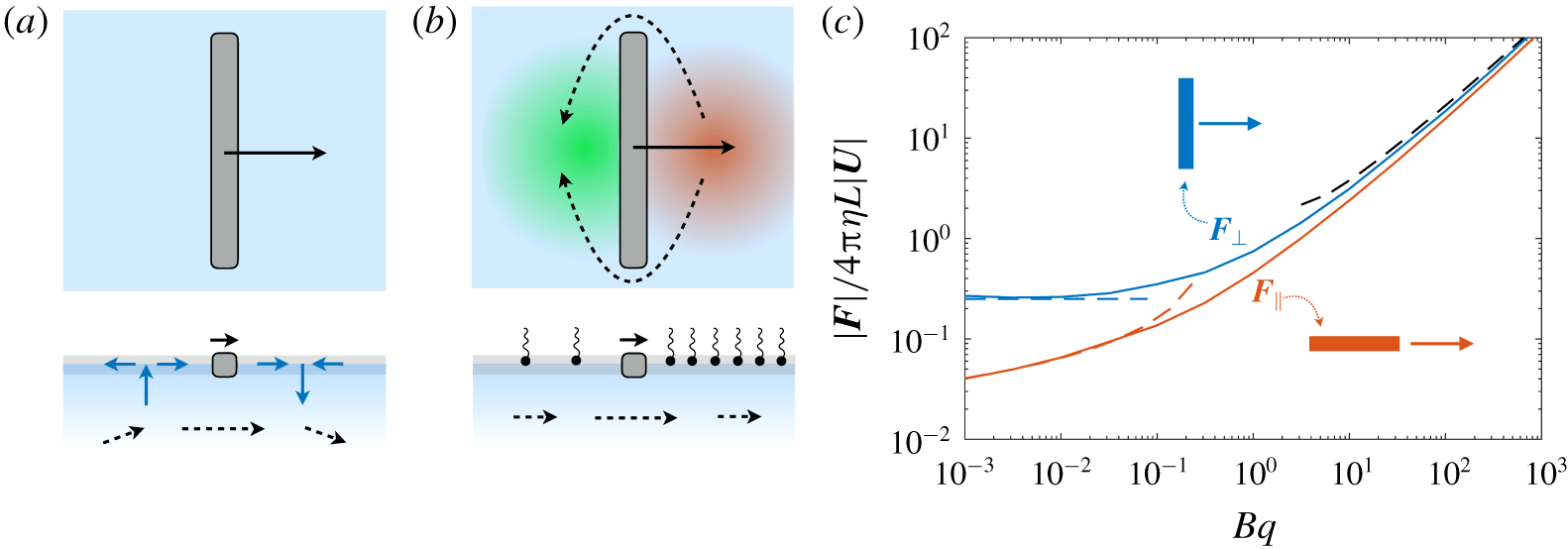
Figure 24. (a) A rod translating perpendicular to its long axis on a clean interface, shown in top and side views. The surface velocity field has a non-zero divergence ahead and behind the rod, and the bulk velocity field is three-dimensional. (b) Insoluble surfactants drive reverse Marangoni flows that render monolayers incompressible (see § 3.3.2 and figure 11), setting up surface and bulk flows on length scales comparable to the rod length. Surface incompressibility thus imparts a larger drag than a clean interface even when the surfactant is surface inviscid ( $Bq\rightarrow 0$
), and impacts
$Bq\rightarrow 0$
), and impacts $\boldsymbol{F}_{\bot }$
more strongly than
$\boldsymbol{F}_{\bot }$
more strongly than $\boldsymbol{F}_{\Vert }$
. (c) Translational resistance coefficient of long rods in incompressible monolayers (Levine et al.
Reference Levine, Liverpool and MacKintosh2004) with asymptotic scalings in dashed lines following (4.168), (4.169) and (4.170).
$\boldsymbol{F}_{\Vert }$
. (c) Translational resistance coefficient of long rods in incompressible monolayers (Levine et al.
Reference Levine, Liverpool and MacKintosh2004) with asymptotic scalings in dashed lines following (4.168), (4.169) and (4.170).
By contrast, the drag for subphase-dominant systems (particularly, when $d\ll \ell _{SD}\ll L$
),
$d\ll \ell _{SD}\ll L$
),
 $$\begin{eqnarray}\boldsymbol{F}_{\Vert }(Bq\ll 1)=-\frac{\unicode[STIX]{x03C0}\unicode[STIX]{x1D702}L\boldsymbol{U}}{\ln (0.48/Bq)},\end{eqnarray}$$
resembles the drag on a rod moving in a bulk fluid (4.167), but with an effective width of $\ell _{SD}$
instead of
$\ell _{SD}$
instead of $d$
. The bulk fluid under the rod does not ‘see’ the smaller length scale
$d$
. The bulk fluid under the rod does not ‘see’ the smaller length scale $d$
, and provides bulk viscous resistance to an ‘effective’ rod of width comparable to the 2-D-to-3-D cross-over length scale
$d$
, and provides bulk viscous resistance to an ‘effective’ rod of width comparable to the 2-D-to-3-D cross-over length scale $\ell _{SD}$
. The most striking difference with 3-D fluids, however, occurs in perpendicular translation when
$\ell _{SD}$
. The most striking difference with 3-D fluids, however, occurs in perpendicular translation when $Bq\ll 1$
:
$Bq\ll 1$
:
 $$\begin{eqnarray}\boldsymbol{F}_{\bot }(Bq\ll 1)=-\unicode[STIX]{x03C0}\unicode[STIX]{x1D702}L\boldsymbol{U}.\end{eqnarray}$$
The drag on a rod moving broadside-on becomes much larger than $\boldsymbol{F}_{\Vert }$
, owing to surface incompressibility. On a clean interface (or on a compressible monolayer with instantaneous adsorption/desorption),
$\boldsymbol{F}_{\Vert }$
, owing to surface incompressibility. On a clean interface (or on a compressible monolayer with instantaneous adsorption/desorption), $\unicode[STIX]{x1D6F1}$
remains approximately uniform, and the surface flow has a non-zero divergence ahead and behind the rod (figure 24
a). Insoluble surfactants that impose surface incompressibility (§ 3.3.2) then perturb velocities over the largest dimension of the rod (figure 24
b), giving rise to the linear dependence on
$\unicode[STIX]{x1D6F1}$
remains approximately uniform, and the surface flow has a non-zero divergence ahead and behind the rod (figure 24
a). Insoluble surfactants that impose surface incompressibility (§ 3.3.2) then perturb velocities over the largest dimension of the rod (figure 24
b), giving rise to the linear dependence on $L$
.
$L$
.
5 Additional complexities with real-world surfactants
We have thus far treated surfactant monolayers in a way that is natural to most fluid mechanicians – as featureless continuum materials, isotropic and homogeneous. While some multi-component monolayers do form homogeneous mixtures – as do miscible liquids and dissolving solutes in 3-D liquids – some surfactant species may associate with each other, or phase separate to form heterogeneous monolayers more akin to emulsions or dispersions. Even single-component monolayers often exhibit non-trivial morphologies, for example, forming condensed phases with liquid crystalline order that coexist with disordered phases. Monolayers in phase coexistence typically consist of ‘grains’ of one phase dispersed in another, acting like dilute dispersions at low surface pressure, then forming grainy, poly-crystalline phases or jammed suspensions (like compressed emulsions or suspensions) upon further compression, depending on the details and dynamics of compression and domain relaxation.
In what follows, we briefly describe some aspects that give surfactant monolayers additional richness and complexity. Section 5.1 describes the unexpectedly rich phase behaviour and morphologies that arise in even simple surfactant monolayers, and how those can be understood in terms of the characteristics of the surfactants themselves. Section 5.2 then addresses how monolayer heterogeneities and anisotropies impact the surface rheology and therefore the fluid dynamics of such systems. In many cases, these surface rheologies can be understood by analogy with three-dimensional non-Newtonian fluids: suspensions and emulsions with effective viscosities, surface viscoelasticity, surface shear thinning and surface yield stresses. New phenomena arise in surface rheology as well, as described in § 5.3: surface rheology very often depends exponentially on surface pressure, which leads to qualitative differences in flow phenomena that would not be expected by a fluid mechanician accustomed to thinking about incompressible, constant-viscosity liquids.
5.1 Phase behaviour of surfactant monolayers
In describing $\unicode[STIX]{x1D6F1}$
–
$\unicode[STIX]{x1D6F1}$
– $\unicode[STIX]{x1D6E4}$
isotherms in § 2 and table 1, we introduced the simplest of phase transitions: surfactants that experience intermolecular attractions (
$\unicode[STIX]{x1D6E4}$
isotherms in § 2 and table 1, we introduced the simplest of phase transitions: surfactants that experience intermolecular attractions ( $\unicode[STIX]{x1D6FD}>0$
) undergo a phase transformation from a gaseous (G) phase at very low surface concentration
$\unicode[STIX]{x1D6FD}>0$
) undergo a phase transformation from a gaseous (G) phase at very low surface concentration $\unicode[STIX]{x1D6E4}$
to a disordered liquid phase (‘liquid expanded’, or LE), frequently with G/LE phase coexistence over a range of
$\unicode[STIX]{x1D6E4}$
to a disordered liquid phase (‘liquid expanded’, or LE), frequently with G/LE phase coexistence over a range of $\unicode[STIX]{x1D6E4}$
, shown in figure 25(d). Compression to higher
$\unicode[STIX]{x1D6E4}$
, shown in figure 25(d). Compression to higher $\unicode[STIX]{x1D6E4}$
often reveals phase behaviours (figure 25) that are significantly richer than the simple gas–liquid transition described by the van der Waals or Frumkin isotherms, forming a host of additional condensed phases with various translational and orientational ordering (Knobler & Desai Reference Knobler and Desai1992; Kaganer et al.
Reference Kaganer, Möhwald and Dutta1999).
$\unicode[STIX]{x1D6E4}$
often reveals phase behaviours (figure 25) that are significantly richer than the simple gas–liquid transition described by the van der Waals or Frumkin isotherms, forming a host of additional condensed phases with various translational and orientational ordering (Knobler & Desai Reference Knobler and Desai1992; Kaganer et al.
Reference Kaganer, Möhwald and Dutta1999).
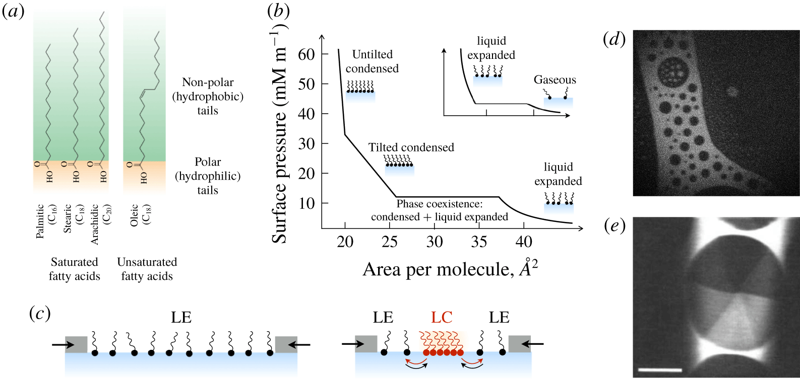
Figure 25. (a) Fatty acids consist of a (hydrophilic) carboxylic acid headgroup and a (hydrophobic) hydrocarbon tail. The longer the hydrocarbon tail, the lower its solubility in water and the stronger the van der Waals attractions with adjacent fatty acids. Saturated hydrocarbon tails pack well with each other, whereas unsaturated tails (e.g. oleic acid, with a double bond at the ninth carbon) are ‘kinked’ and frustrate packing. (b) Generalized isotherm of an insoluble monolayer of saturated fatty acids, adapted from Kaganer et al. (Reference Kaganer, Möhwald and Dutta1999). Monolayers form a gaseous phase at extremely low concentration (inset), which condenses to form a disordered, liquid expanded (LE) phase when compressed. At higher surface concentrations, a phase transition occurs from the LE phase to one of various liquid condensed (LC) phases with different liquid crystalline order, and even further phase transitions at higher concentrations (here to an untilted, condensed phase). (c) Cartoon showing transition between a disordered, low-density phase (e.g. LE or gaseous) to phase coexistence with a higher-density phase (e.g. LE/LC or gas/LE). (d) Fluorescence micrograph showing gas/LE phase coexistence of the phospholipid DPPC (courtesy of Dr I. Williams). (e) Polarized micrograph of LE–LC phase coexistence between methyl eicosanoate(C $_{20}$
). Within the LC domain, the six different brightness levels correspond to six distinct orientations of the packed tails, which in turn reveal the hexagonal headgroup lattice (from Knobler & Desai (Reference Knobler and Desai1992)).
$_{20}$
). Within the LC domain, the six different brightness levels correspond to six distinct orientations of the packed tails, which in turn reveal the hexagonal headgroup lattice (from Knobler & Desai (Reference Knobler and Desai1992)).
Perhaps the simplest, ‘canonical’ surfactants are saturated fatty alcohols or acids, shown in figure 25(a), which consist of a linear alkyl chain as a hydrophobic tail, and a small polar group (e.g. alcohol or carboxylic acid) as the hydrophilic head. Figure 25(b) depicts a generic isotherm for Langmuir monolayers of saturated fatty acids or alcohols. When a disordered liquid (LE) is compressed past a particular concentration $\unicode[STIX]{x1D6E4}_{\ast }$
(or below an area per molecule
$\unicode[STIX]{x1D6E4}_{\ast }$
(or below an area per molecule $A_{\ast }=1/\unicode[STIX]{x1D6E4}_{\ast }$
), ‘liquid condensed’ (LC) domains with liquid crystalline ordering nucleate and grow within the continuous, disordered LE phase. Within each LC domain, the hydrophilic headgroups form a hexagonal lattice, and the hydrophobic tails tilt towards neighbouring tails to maximize attractive van der Waals interactions (figure 25
e). The difference between surfactant concentrations (
$A_{\ast }=1/\unicode[STIX]{x1D6E4}_{\ast }$
), ‘liquid condensed’ (LC) domains with liquid crystalline ordering nucleate and grow within the continuous, disordered LE phase. Within each LC domain, the hydrophilic headgroups form a hexagonal lattice, and the hydrophobic tails tilt towards neighbouring tails to maximize attractive van der Waals interactions (figure 25
e). The difference between surfactant concentrations ( $\unicode[STIX]{x1D6E4}_{C}$
and
$\unicode[STIX]{x1D6E4}_{C}$
and $\unicode[STIX]{x1D6E4}_{E}$
) in the LC and LE phases imparts different electrostatic dipole densities to the two phases, giving rise to dipole-dipole repulsions between LC domains that effectively stabilize the dispersion against coalescence (McConnell Reference McConnell1991). Increasing
$\unicode[STIX]{x1D6E4}_{E}$
) in the LC and LE phases imparts different electrostatic dipole densities to the two phases, giving rise to dipole-dipole repulsions between LC domains that effectively stabilize the dispersion against coalescence (McConnell Reference McConnell1991). Increasing $\unicode[STIX]{x1D6E4}$
(or decreasing
$\unicode[STIX]{x1D6E4}$
(or decreasing $A$
) grows LC grains at the expense of LE, and ultimately forms a fully LC phase. The LE–LC ‘condensation’ process reflects a balance between favourable interactions between tilted tails, and unfavourable entropic losses: headgroups lose translational entropy by forming lattices, whereas tails lose orientational entropy by tilting. In this balance, lengthening the alkyl tail of a surfactant increases the van der Waals ‘benefit’ to condensation, with relatively small entropic penalties. Consequently, the melting temperature of the LC phase increases with hydrocarbon tail length, typically by 5–10 K per carbon (Bibo & Peterson Reference Bibo and Peterson1990).
$A$
) grows LC grains at the expense of LE, and ultimately forms a fully LC phase. The LE–LC ‘condensation’ process reflects a balance between favourable interactions between tilted tails, and unfavourable entropic losses: headgroups lose translational entropy by forming lattices, whereas tails lose orientational entropy by tilting. In this balance, lengthening the alkyl tail of a surfactant increases the van der Waals ‘benefit’ to condensation, with relatively small entropic penalties. Consequently, the melting temperature of the LC phase increases with hydrocarbon tail length, typically by 5–10 K per carbon (Bibo & Peterson Reference Bibo and Peterson1990).
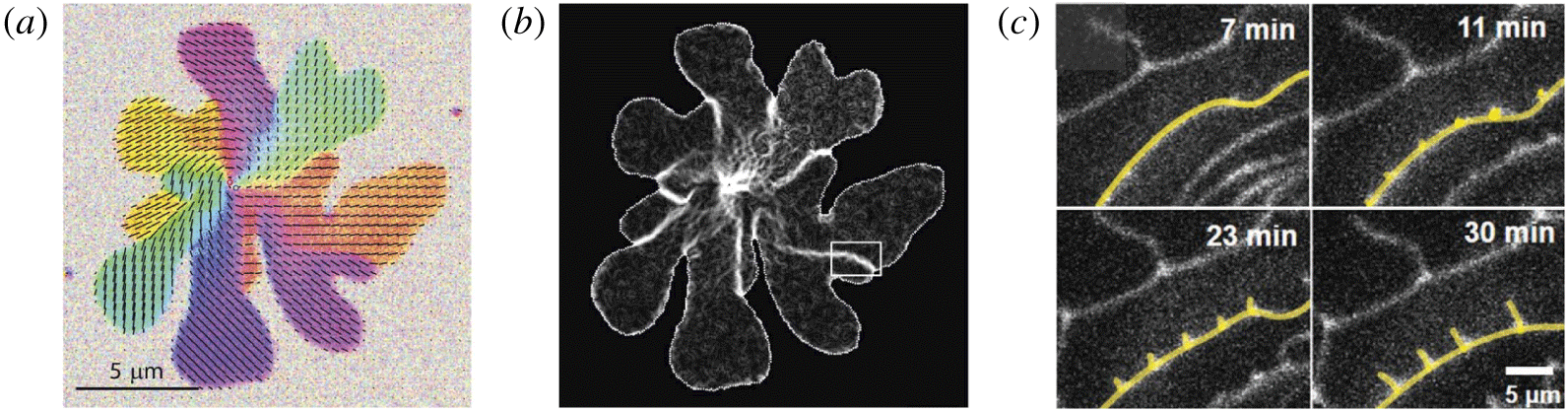
Figure 26. (a) Tilted DPPC tail groups within an LC domain form discrete patches, within which tails are oriented in the same direction. The tilt orientation jumps by 60 $^{\circ }$
from patch to patch, to accommodate the frustration between the tendency of tilt orientation to precess and the tendency of the hexagonal headgroup lattice to maintain its order. (b) Bright lines indicate boundaries between patches of aligned tilt, across which tailgroup orientation abruptly changes. These high-energy lines exert a line tension internal to the drop, effectively ‘pulling’ in invaginations at the domain boundary. (a,b) Reproduced from Dreier, Brewer & Simonsen (Reference Dreier, Brewer and Simonsen2012). (c) New tilt grain boundary lines form and grow in LC DPPC domain arms that had been stretched significantly. From Kim et al. (Reference Kim, Choi, Zasadzinski and Squires2018).
$^{\circ }$
from patch to patch, to accommodate the frustration between the tendency of tilt orientation to precess and the tendency of the hexagonal headgroup lattice to maintain its order. (b) Bright lines indicate boundaries between patches of aligned tilt, across which tailgroup orientation abruptly changes. These high-energy lines exert a line tension internal to the drop, effectively ‘pulling’ in invaginations at the domain boundary. (a,b) Reproduced from Dreier, Brewer & Simonsen (Reference Dreier, Brewer and Simonsen2012). (c) New tilt grain boundary lines form and grow in LC DPPC domain arms that had been stretched significantly. From Kim et al. (Reference Kim, Choi, Zasadzinski and Squires2018).
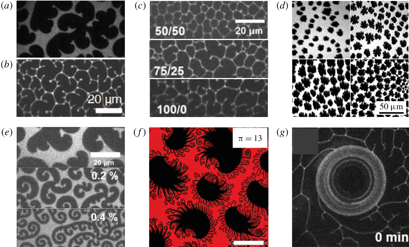
Figure 27. (a,b) The phospholipid Dipalmitoylphostphatidylcholine (DPPC) in (a) LC/LE coexistence and (b) polycrystalline, fully LC phase, from Kim et al. (Reference Kim, Choi, Zasadzinski and Squires2018). Natural DPPC forms LC domains that wind in a counter-clockwise fashion, owing to the chiral attachment of the two hydrocarbon tails. (c) The chirality of domains within an LC DPPC monolayer depends on the ratio of right- to left-handed DPPC molecules (from Kim et al. (Reference Kim, Choi, Zasadzinski and Squires2018)). (d) Palmitic acid co-crystallizes with DPPC to form stiff inclusions, here dispersed by a disordered phase of the unsaturated lipid POPG (from Ding, Warriner & Zasadzinski (Reference Ding, Warriner and Zasadzinski2002)). (e) Cholesterol is ‘line active’ for DPPC, promoting the growth of thinner LC grains that wind more tightly (from Kim et al. (Reference Kim, Choi, Zell, Squires and Zasadzinski2013)). (f) DPPC/hexadecanol/cholesterol mixtures form eerily beautiful grains in LC/LE coexistence, consisting of a DPPC/HD co-crystallized core, surrounded by wispy, spiralling DPPC/cholesterol arms (from Sachan et al. (Reference Sachan, Choi, Kim, Tang, Hwang, Lee, Squires and Zasadzinski2017)). (f) An LC-DPPC monolayer that is steadily deformed by a rotating microfabricated ‘button’, reveals a surface yield stress: the monolayer flows within the high-stress region near the button, but is stationary outside a yield radius (from Kim et al. (Reference Kim, Choi, Zasadzinski and Squires2018)).
When facing a fully LC phase, the fluid mechanician might breathe a sigh of relief, in the hopes that LC monolayers act like familiar homogeneous liquids. That fluid mechanician should prepare for disappointment, however. Such LC phases are generally polycrystalline, consisting of compressed LC grains (e.g. figure 27 b), each of which has a headgroup lattice that is oriented differently from its neighbours; moreover, tail groups generally tilt in one of six energetically equivalent directions relative to the lattice (figures 25 e and 26 a,b). Even grains whose headgroup lattices were aligned would only coalesce if their tail tilts were also aligned. The complexity continues: upon further compression, LC monolayers may go through other phase transitions, to any of a veritable menagerie of liquid crystalline phases.
Double bonds within the alkyl tail change the phase behaviour rather dramatically. For example, oleic acid is chemically nearly identical to stearic acid, but with one double bond that ‘kinks’ the tail in a way that frustrates packing with neighbouring tails and therefore weakens van der Waals attractions (figure 25 a). Unsaturated tails therefore discourage or even prevent liquid condensed phases from forming. In fact, 2-D surfactant ‘dispersions’ can be designed by spreading a mixture of saturated and unsaturated fatty acids or alcohols: upon compression, saturated lipids condense to form LC grains, but unsaturated lipids remain in a continuous LE phase (figure 27 e, from Ding et al. (Reference Ding, Warriner and Zasadzinski2002)).
Phospholipids – the primary surfactants that form the membranes of cells, vesicles and organelles – show even more complex phase behaviour than fatty acids. This complexity arises in part because phospholipids have two hydrocarbon tails; additionally, these tails attach to the headgroup in a chiral fashion. As with fatty acids, headgroups condense to form hexagonal lattices, and (saturated) tails tilt (some towards nearest neighbours, others towards next nearest neighbours). The chiral attachment of each pair of tails, however, promotes a gradual precession of tail tilt direction, causing LC domains to ‘wind’ with a particular handedness (see, e.g. the counter-clockwise spiral arms in LC domains of the common phospholipid DPPC in figure 27 a).
Frustration arises between the packing preferences of the heads and the tails, however, since the tail tilt orientation can only precess by straining the headgroup lattice. Since each LC domain represents a single crystal of hexagonally packed headgroups, this frustration becomes untenable once LC domains grow large enough. LC DPPC domains ultimately resolve this tension between ordered headgroup lattices and winding tailgroup tilt orientation by forming tilt mosaics (figure 26). Within each ‘patch’ of the mosaic, tail groups tilt in one of 6 directions relative to the HCP lattice, and precess gradually (Dreier et al. Reference Dreier, Brewer and Simonsen2012). Tilt orientation changes discontinuously from one patch of the mosaic to the next, however, across tilt–grain boundary lines where tilt orientations are disordered and thus energetically more costly. These high-energy defects exert additional ‘line tensions’ within the domain. Stretching these LC domains significantly disrupts the balance in frustration between the headgroup lattice and tail tilt precession, and can trigger the nucleation and growth of new tilt grain defects (figure 26 c) that stabilize the stretched LC arms against shape relaxation, akin to plastic deformations in solids.
LC DPPC domain shapes thus reflect a variety of competing forces (Mohwald Reference Mohwald1990; McConnell Reference McConnell1991; Dreier et al. Reference Dreier, Brewer and Simonsen2012): dipole–dipole repulsions within each domain tend to favour elongation of each domain, whereas the line tension introduced by the higher energetic state of surfactants at the LC/LE boundary acts to reduce the perimeter to area ratio. Tilt orientation precession promotes the chiral winding of spiral arms, which competes with the headgroup lattice trying to maintain its preferred crystalline order. Frustration between tilt precession and headgroup lattice ordering is resolved by high-energy tilt grain boundaries that exert their own line tension within each domain, ‘pulling inwards’ at various points along the domain boundary, causing the concave ‘kinks’ and invaginations along the domain boundary.
Figure 27 highlights a small sliver of the wild menagerie of morphologies formed by condensed mixtures of DPPC and other insoluble surfactants. The chirality of LC DPPC domains is apparent in both LC/LE coexistence (figure 27 a) and in the fully condensed, polycrystalline LC phase (figure 27 a), growing with the ratio of left- to right-handed DPPC in the mixture (figure 27 c), as studied by Kim et al. (Reference Kim, Choi, Zasadzinski and Squires2018).
Saturated fatty acids or alcohols may co-crystallize with LC phospholipids, since their small headgroups enable them to insert into the headgroup lattice without deforming it significantly, while reaping the benefits of tail–tail packing. Such co-crystallization tends to stiffen these domains. Just like fatty acids and alcohols, unsaturated phospholipids generally don’t form LC phases, and so can be used to control the area fraction of LC/LE dispersions (figure 27 d, from Ding et al. (Reference Ding, Warriner and Zasadzinski2002)).
By contrast, cholesterols have small headgroups but big ring ‘tails’ that act to promote defects within LC grains. Moreover, just as surfactants lower surface energy when they adsorb to 2-D interfaces between 3-D liquids, ‘line-actant’ molecules adsorb to 1-D boundaries of 2-D surfactant domains to lower line energy (Trabelsi et al. Reference Trabelsi, Zhang, Lee and Schwartz2008). Cholesterol is a line actant for LC-DPPC (Kim et al. Reference Kim, Choi, Zell, Squires and Zasadzinski2013) and promotes thinner LC spiral arms that wind more tightly (figure 27 e). Mixing all three components (phospholipid, fatty alcohol and cholesterol) forms LC grains that are as complex as they are beautiful: stiff ‘cores’ of DPPC–hexadecanol form first, followed by wispy spirals of DPPC–cholesterol mixtures (figure 27 f, from Sachan et al. (Reference Sachan, Choi, Kim, Tang, Hwang, Lee, Squires and Zasadzinski2017)).
These examples serve only to give a very cursory sense of the incredibly rich variety of monolayers, phases and domains that form in even seemingly simple systems with one or two small-molecule surfactants. Additional complexities arise when solutes in the subphase interact with surfactants in the monolayer. Multivalent ions may electrostatically bridge multiple ionic surfactants: for example, calcium ions (Ca $^{2+}$
) adsorb to two stearic acid molecules, stiffening monolayers (Ghaskadvi, Carr & Dennin Reference Ghaskadvi, Carr and Dennin1999) and even growing multilayer films of calcium distearate (de Ruiter et al.
Reference de Ruiter, Tjerkstra, Duits and Mugele2011). However exotic and beautiful this process may appear to the curious scientist, those who shower with ‘hard’ water call it soap scum.
$^{2+}$
) adsorb to two stearic acid molecules, stiffening monolayers (Ghaskadvi, Carr & Dennin Reference Ghaskadvi, Carr and Dennin1999) and even growing multilayer films of calcium distearate (de Ruiter et al.
Reference de Ruiter, Tjerkstra, Duits and Mugele2011). However exotic and beautiful this process may appear to the curious scientist, those who shower with ‘hard’ water call it soap scum.
5.2 Rheological implications of surface heterogeneities
Because surfactant monolayers are frequently heterogeneous (e.g. figure 27), determining their rheological properties and predicting their mechanical response to flows and stresses can be challenging. A detailed discussion of the complex structure and non-Newtonian rheology of surfactant monolayers is beyond the scope of this work, and recent reviews provide a more exhaustive survey of the state of the field (Fuller & Vermant Reference Fuller and Vermant2012; Langevin Reference Langevin2014; Jaensson & Vermant Reference Jaensson and Vermant2018). Instead, in what follows, we merely outline aspects of 2-D heterogeneous monolayers that qualitatively resemble familiar 3-D systems, and where intuition and physical concepts from classical fluid dynamics can be borrowed to describe and design these 2-D systems.
5.2.1 Line tension: liquid crystalline domains as 2-D drops
Recall from § 2.1 that molecules on the interface between 3-D fluids are in an energetically unfavourable state, giving rise to surface tension (figure 2). The 2-D analogue occurs on the ‘interface’ between surfactant phases – LC domain boundaries are higher energy and give rise to a line tension $\unicode[STIX]{x1D706}$
, or energy per unit perimeter. The attractive interaction energy between molecules in the condensed phase must be
$\unicode[STIX]{x1D706}$
, or energy per unit perimeter. The attractive interaction energy between molecules in the condensed phase must be $O(k_{B}T)$
. Condensation involves moving molecules from the disordered phase to LC and therefore requires an energy
$O(k_{B}T)$
. Condensation involves moving molecules from the disordered phase to LC and therefore requires an energy ${\sim}k_{B}T$
per molecule. Molecules pack with a line density of about one per nanometre, giving
${\sim}k_{B}T$
per molecule. Molecules pack with a line density of about one per nanometre, giving $\unicode[STIX]{x1D706}\sim k_{B}T/\text{nm}\sim \text{pN}$
.
$\unicode[STIX]{x1D706}\sim k_{B}T/\text{nm}\sim \text{pN}$
.
Just like surface tension acts to restore the equilibrium shapes of deformed, 3-D emulsion drops or bubbles, the LC line tension acts to force deformed LC domains to relax back to their equilibrium shapes, at a rate that is limited by the surface viscosity of the LC phase when $Bq\gg 1$
(or by subphase viscosity when
$Bq\gg 1$
(or by subphase viscosity when $Bq\ll 1$
). Indeed,
$Bq\ll 1$
). Indeed, $\unicode[STIX]{x1D706}$
can be identified by measuring the relaxation dynamics of stretched LC ‘droplets’ (Mann et al.
Reference Mann, Hénon, Langevin, Meunier and Léger1995; Trabelsi et al.
Reference Trabelsi, Zhang, Lee and Schwartz2008). When interface dominant (
$\unicode[STIX]{x1D706}$
can be identified by measuring the relaxation dynamics of stretched LC ‘droplets’ (Mann et al.
Reference Mann, Hénon, Langevin, Meunier and Léger1995; Trabelsi et al.
Reference Trabelsi, Zhang, Lee and Schwartz2008). When interface dominant ( $Bq\gg 1$
), balancing the line tension force (
$Bq\gg 1$
), balancing the line tension force ( ${\sim}\unicode[STIX]{x1D706}$
) with the surface viscous force (
${\sim}\unicode[STIX]{x1D706}$
) with the surface viscous force ( ${\sim}\unicode[STIX]{x1D702}_{s}{\dot{R}}$
, with
${\sim}\unicode[STIX]{x1D702}_{s}{\dot{R}}$
, with $R$
the characteristic domain length scale) gives a characteristic relaxation time
$R$
the characteristic domain length scale) gives a characteristic relaxation time
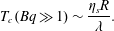 $$\begin{eqnarray}T_{c}(Bq\gg 1)\sim \frac{\unicode[STIX]{x1D702}_{s}R}{\unicode[STIX]{x1D706}}.\end{eqnarray}$$
By contrast, the bulk fluid offers the dominant viscous resistance ( ${\sim}\unicode[STIX]{x1D702}R{\dot{R}}$
) when subphase dominant (
${\sim}\unicode[STIX]{x1D702}R{\dot{R}}$
) when subphase dominant ( $Bq\ll 1$
), giving
$Bq\ll 1$
), giving
 $$\begin{eqnarray}T_{c}(Bq\ll 1)\sim \frac{\unicode[STIX]{x1D702}R^{2}}{\unicode[STIX]{x1D706}}.\end{eqnarray}$$
Extending the analogy, fully LC phases act like compressed emulsions – like two-dimensional mayonnaise. Interlocking domains impart a yield stress to fully LC monolayers, enabling them to sustain elastic stresses over system-spanning length scales. The dynamics of LC domains is then described by a surface capillary number,
 $$\begin{eqnarray}Ca_{s}=\frac{\unicode[STIX]{x1D702}_{s}V}{\unicode[STIX]{x1D706}},\end{eqnarray}$$
which for domains of some size $R$
, sheared at rate
$R$
, sheared at rate $\dot{\unicode[STIX]{x1D6FE}}$
or frequency
$\dot{\unicode[STIX]{x1D6FE}}$
or frequency $\unicode[STIX]{x1D714}$
, becomes
$\unicode[STIX]{x1D714}$
, becomes
 $$\begin{eqnarray}Ca_{s}=\frac{\unicode[STIX]{x1D702}_{s}R\unicode[STIX]{x1D714}}{\unicode[STIX]{x1D706}},\quad \text{or}\quad Ca_{s}=\frac{\unicode[STIX]{x1D702}_{s}R\dot{\unicode[STIX]{x1D6FE}}}{\unicode[STIX]{x1D706}}.\end{eqnarray}$$
Surface capillary stresses dominate at low frequencies, acting to restore domain shapes and imparting a solid-like response. By contrast, viscous stresses dominate at high frequencies, as the LC phase resists deformation within each grain. From the cross-over frequency $\unicode[STIX]{x1D714}_{c}$
, the line tension can be identified (Choi et al.
Reference Choi, Steltenkamp, Zasadzinski and Squires2011).
$\unicode[STIX]{x1D714}_{c}$
, the line tension can be identified (Choi et al.
Reference Choi, Steltenkamp, Zasadzinski and Squires2011).
The healing of deformed LC monolayers, however, is qualitatively different from traditional yield-stress materials. Unlike 3-D drops, elongated domains do not ‘pinch off’ due to capillary forces. The classic Rayleigh–Plateau instability is suppressed by the absence of out-of-plane curvature of LC domains. Even thread-like domains are therefore stable for long times (Trabelsi et al. Reference Trabelsi, Zhang, Lee and Schwartz2008). Deformed LC phases heal via line-tension-driven relaxation of highly stretched domains back to more compact equilibrium shapes. Additional viscous losses may be incurred in sliding domains against each other, or in irreversible topological rearrangements. The net effect is a viscoelastic recovery – one that can take hours (Choi et al. Reference Choi, Steltenkamp, Zasadzinski and Squires2011).
5.2.2 Two-dimensional ‘suspensions’ of condensed domains: effective surface viscosities
Liquid condensed phases are typically much stiffer rheologically than LE phases. Langmuir monolayers in LE–LC phase coexistence can thus be treated as a suspension of ‘stiff’ 2-D particles dispersed in a continuous ‘liquid’. In fact, Ding et al. (Reference Ding, Warriner and Zasadzinski2002) measured the effective surface shear viscosity of DPPC–palmitic acid mixtures over a wide range of LE–LC coexistence, finding a power-law divergence
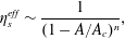 $$\begin{eqnarray}\unicode[STIX]{x1D702}_{s}^{eff}\sim \frac{1}{(1-A/A_{c})^{n}},\end{eqnarray}$$
as the domain area $A$
approached some critical area
$A$
approached some critical area $A_{c}$
. Analogous behaviour had been known and shown in 3-D suspensions (Brady Reference Brady1993; Stickel & Powell Reference Stickel and Powell2005).
$A_{c}$
. Analogous behaviour had been known and shown in 3-D suspensions (Brady Reference Brady1993; Stickel & Powell Reference Stickel and Powell2005).
In system where domains are effectively rigid inclusions suspended in an incompressible, continuous phase that is surface viscous enough to be interface dominant ( $Bq\gg 1$
), the subphase may be ignored and the monolayer rheology corresponds to the Einstein viscosity correction in two dimensions. This classic problem in low-Reynolds-number hydrodynamics (Brady Reference Brady1983) gives the effective shear viscosity of a 2-D suspension with a domain area fraction
$Bq\gg 1$
), the subphase may be ignored and the monolayer rheology corresponds to the Einstein viscosity correction in two dimensions. This classic problem in low-Reynolds-number hydrodynamics (Brady Reference Brady1983) gives the effective shear viscosity of a 2-D suspension with a domain area fraction $\unicode[STIX]{x1D719}\ll 1$
to be
$\unicode[STIX]{x1D719}\ll 1$
to be
 $$\begin{eqnarray}\unicode[STIX]{x1D702}_{s}^{eff}(Bq\gg 1)=\unicode[STIX]{x1D702}_{s}^{c}(1+2\unicode[STIX]{x1D719}),\end{eqnarray}$$
where $\unicode[STIX]{x1D702}_{s}^{c}$
is the surface shear viscosity of the continuous phase.
$\unicode[STIX]{x1D702}_{s}^{c}$
is the surface shear viscosity of the continuous phase.
Additionally, surfactant monolayers are far more compressible than 3-D fluids, and the flow of a compressible 2-D ‘fluid’ around incompressible domains dissipates excess surface-viscous stresses. The ‘Einstein correction’ to the 2-D dilatational viscosity is (Khair Reference Khair2006)
 $$\begin{eqnarray}\unicode[STIX]{x1D705}_{s}^{eff}(Bq\gg 1)=\frac{\unicode[STIX]{x1D705}_{s}^{c}+\unicode[STIX]{x1D719}\unicode[STIX]{x1D702}_{s}^{c}}{1-\unicode[STIX]{x1D719}},\end{eqnarray}$$
where $\unicode[STIX]{x1D705}_{s}^{c}$
is the dilatational surface viscosity of the continuous phase. Notably,
$\unicode[STIX]{x1D705}_{s}^{c}$
is the dilatational surface viscosity of the continuous phase. Notably, $\unicode[STIX]{x1D705}_{s}^{eff}$
depends on the surface shear viscosity of the continuous phase,
$\unicode[STIX]{x1D705}_{s}^{eff}$
depends on the surface shear viscosity of the continuous phase, $\unicode[STIX]{x1D702}_{s}^{c}$
. Even if
$\unicode[STIX]{x1D702}_{s}^{c}$
. Even if $\unicode[STIX]{x1D705}_{s}^{c}$
is immeasurably small, rigid inclusions modify surface flows in a manner that imparts an effective dilatational viscosity
$\unicode[STIX]{x1D705}_{s}^{c}$
is immeasurably small, rigid inclusions modify surface flows in a manner that imparts an effective dilatational viscosity $\unicode[STIX]{x1D705}_{s}^{eff}\approx \unicode[STIX]{x1D719}\unicode[STIX]{x1D702}_{s}^{c}$
to the monolayer.
$\unicode[STIX]{x1D705}_{s}^{eff}\approx \unicode[STIX]{x1D719}\unicode[STIX]{x1D702}_{s}^{c}$
to the monolayer.
Stiff inclusions suspended in an inviscid monolayer, e.g. a dispersion of repulsive colloidal microparticles on a clean fluid interface, might also impart an effective surface shear viscosity (Buttinoni et al. Reference Buttinoni, Zell, Squires and Isa2015). The colloids do not deform, and the suspending fluid interface is clean and therefore offers no surface-viscous resistance. Viscous dissipation in the subphase fluid due to the relative motion of colloids against interparticle potentials appears as a ‘surface viscosity’ of the 2-D colloidal layer.
5.2.3 Apparent surface dilatational rheology during phase coexistence
Section 4.2.1 described how dynamic adsorption and desorption of soluble surfactants as an interface is compressed relaxes surface stresses, thereby diminishing the dilatational modulus $E$
and imparting an apparent surface viscosity
$E$
and imparting an apparent surface viscosity $\unicode[STIX]{x1D705}_{s}^{app}\sim E_{0}\unicode[STIX]{x1D70F}_{s}$
. Similar processes can arise within monolayers at phase coexistence, where exchange between condensed and expanded phases plays a role analogous to adsorption/desorption. To illustrate, we treat the kinetics of exchange between phases with a simple adsorption-like model, using
$\unicode[STIX]{x1D705}_{s}^{app}\sim E_{0}\unicode[STIX]{x1D70F}_{s}$
. Similar processes can arise within monolayers at phase coexistence, where exchange between condensed and expanded phases plays a role analogous to adsorption/desorption. To illustrate, we treat the kinetics of exchange between phases with a simple adsorption-like model, using $\unicode[STIX]{x1D6E4}_{C}$
and
$\unicode[STIX]{x1D6E4}_{C}$
and $\unicode[STIX]{x1D6E4}_{E}$
to represent the surface concentration in the condensed and expanded phases, respectively. The total number of molecules is conserved between the two phases,
$\unicode[STIX]{x1D6E4}_{E}$
to represent the surface concentration in the condensed and expanded phases, respectively. The total number of molecules is conserved between the two phases,
 $$\begin{eqnarray}\displaystyle & \displaystyle \frac{1}{A_{E}}\frac{\text{d}(\unicode[STIX]{x1D6E4}_{E}A_{E})}{\text{d}t}=-j_{p}, & \displaystyle\end{eqnarray}$$
 $$\begin{eqnarray}\displaystyle & \displaystyle \frac{1}{A_{C}}\frac{\text{d}(\unicode[STIX]{x1D6E4}_{C}A_{C})}{\text{d}t}=j_{p}, & \displaystyle\end{eqnarray}$$ $j_{p}$
is the net line flux (across domain boundaries) as a result of molecules hopping between phases, and
$j_{p}$
is the net line flux (across domain boundaries) as a result of molecules hopping between phases, and $A_{E}$
and
$A_{E}$
and $A_{C}$
are the areas of the expanded and condensed phase, respectively.
$A_{C}$
are the areas of the expanded and condensed phase, respectively.
Rheologically, we assume that the condensed domains act like rigid inclusions, so that all compressibility (and fluidity) of the heterogeneous monolayer originates in the expanded phase. Under weak sinusoidal surface dilatation at frequency $\unicode[STIX]{x1D714}$
, the surface concentration and area of the expanded phase are perturbed via
$\unicode[STIX]{x1D714}$
, the surface concentration and area of the expanded phase are perturbed via
 $$\begin{eqnarray}\displaystyle & \displaystyle A_{E}(t)=A_{E}^{0}+\unicode[STIX]{x1D6FF}A_{E}\text{e}^{\text{i}\unicode[STIX]{x1D714}t}, & \displaystyle\end{eqnarray}$$
 $$\begin{eqnarray}\displaystyle & \displaystyle \unicode[STIX]{x1D6E4}_{E}(t)=\unicode[STIX]{x1D6E4}_{E}^{0}+\unicode[STIX]{x1D6FF}\unicode[STIX]{x1D6E4}_{E}\text{e}^{\text{i}\unicode[STIX]{x1D714}t}. & \displaystyle\end{eqnarray}$$ $\unicode[STIX]{x1D6E4}_{C}(t)$
is assumed to remain a constant
$\unicode[STIX]{x1D6E4}_{C}(t)$
is assumed to remain a constant $\unicode[STIX]{x1D6E4}_{C}^{0}$
.
$\unicode[STIX]{x1D6E4}_{C}^{0}$
.
Although the exchange flux $j_{p}$
could be diffusion- or kinetically limited, we will assume a simple kinetically limited condensation process, with the flux from either phase proportional to the local concentration:
$j_{p}$
could be diffusion- or kinetically limited, we will assume a simple kinetically limited condensation process, with the flux from either phase proportional to the local concentration:
 $$\begin{eqnarray}j_{E\rightarrow C}=k_{E\rightarrow C}\unicode[STIX]{x1D6E4}_{E},\quad j_{C\rightarrow E}=k_{C\rightarrow E}\unicode[STIX]{x1D6E4}_{C}=j_{C}^{0},\end{eqnarray}$$
so that $j_{E\rightarrow C}=j_{C\rightarrow E}$
at equilibrium. When perturbed via (5.9), the net flux into (or out of) the condensed phase is
$j_{E\rightarrow C}=j_{C\rightarrow E}$
at equilibrium. When perturbed via (5.9), the net flux into (or out of) the condensed phase is
 $$\begin{eqnarray}j_{p}=j_{E\rightarrow C}-j_{C\rightarrow E}=k_{p}\unicode[STIX]{x1D6FF}\unicode[STIX]{x1D6E4}_{E}\text{e}^{\text{i}\unicode[STIX]{x1D714}t},\end{eqnarray}$$
where $k_{p}=j_{C}^{0}/\unicode[STIX]{x1D6E4}_{E}^{0}$
. Perturbations in surface concentration thus relax over a time scale
$k_{p}=j_{C}^{0}/\unicode[STIX]{x1D6E4}_{E}^{0}$
. Perturbations in surface concentration thus relax over a time scale $k_{p}^{-1}$
.
$k_{p}^{-1}$
.
Substituting (5.9) and (5.11) in the conservation equation (5.8a ) gives
 $$\begin{eqnarray}\frac{\text{d}\ln \unicode[STIX]{x1D6E4}_{E}}{\text{d}\ln A_{E}}=-\frac{1}{1-\text{i}\unicode[STIX]{x1D701}_{p}},\end{eqnarray}$$
where
 $$\begin{eqnarray}\unicode[STIX]{x1D701}_{p}=\frac{k_{p}}{\unicode[STIX]{x1D714}}\end{eqnarray}$$
is the ratio of phase change rate to oscillation rate.
When $\unicode[STIX]{x1D701}_{p}\gg 1$
, condensed domains incorporate excess molecules from the expanded phase much faster than
$\unicode[STIX]{x1D701}_{p}\gg 1$
, condensed domains incorporate excess molecules from the expanded phase much faster than $\unicode[STIX]{x1D6E4}$
oscillates, so that the monolayer evolves quasistatically. Conversely, when
$\unicode[STIX]{x1D6E4}$
oscillates, so that the monolayer evolves quasistatically. Conversely, when $\unicode[STIX]{x1D701}_{p}\ll 1$
, compression oscillates so rapidly that little condensation can occur (figure 28).
$\unicode[STIX]{x1D701}_{p}\ll 1$
, compression oscillates so rapidly that little condensation can occur (figure 28).
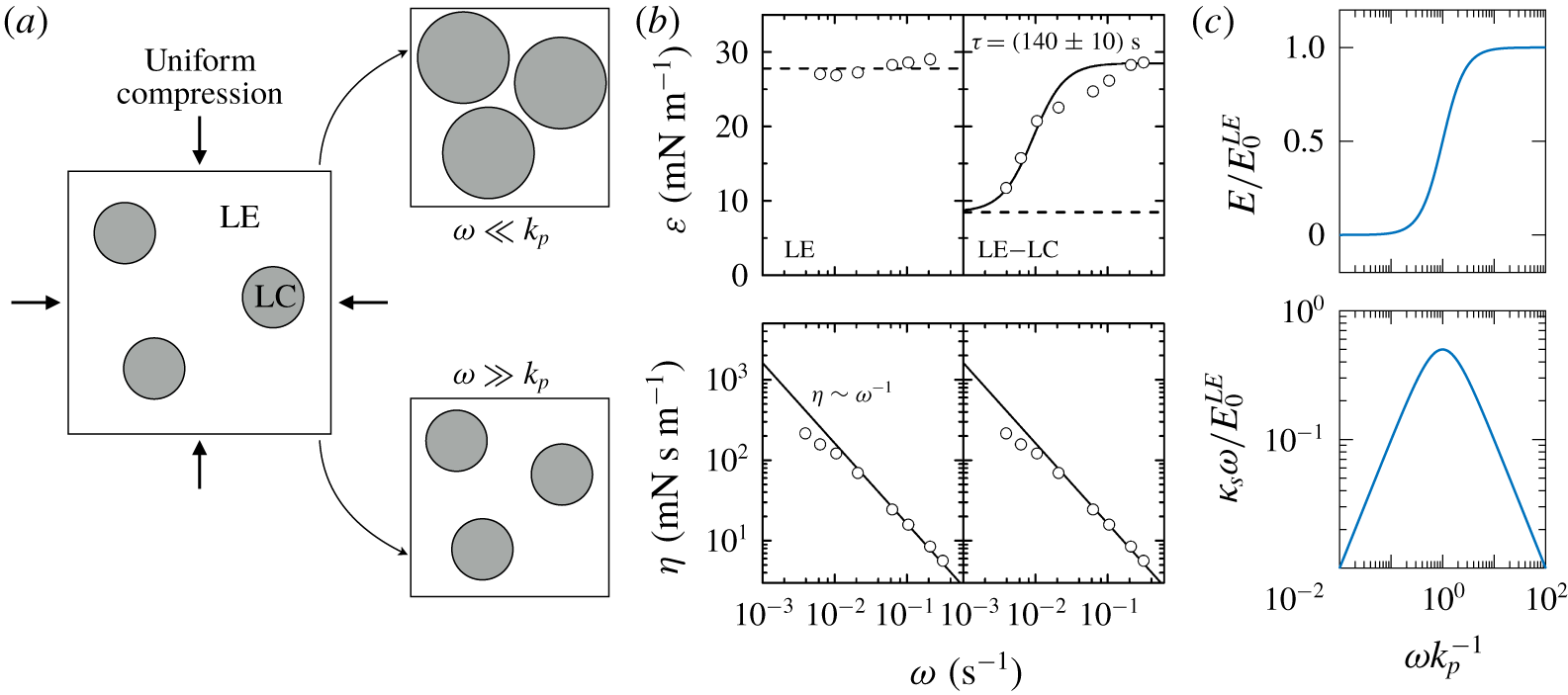
Figure 28. (a) Response of a monolayer with coexisting phases to uniform compression: when $\unicode[STIX]{x1D714}\ll k_{p}$
, domains grow much faster than the rate of compression, and the LE phase offers no elastic resistance. By contrast, when
$\unicode[STIX]{x1D714}\ll k_{p}$
, domains grow much faster than the rate of compression, and the LE phase offers no elastic resistance. By contrast, when $\unicode[STIX]{x1D714}\gg k_{p}$
, the rate of compression exceeds the rate of molecules changing phases, and the LE phase offers a net resistance to compression. (b) Measurements of Arriaga et al. (Reference Arriaga, López-Montero, Ignés-Mullol and Monroy2010) showing elastic and viscous moduli from oscillatory measurements in LE and in coexistence. The solid lines are fit to a Maxwell viscoelastic fluid with characteristic relaxation time
$\unicode[STIX]{x1D714}\gg k_{p}$
, the rate of compression exceeds the rate of molecules changing phases, and the LE phase offers a net resistance to compression. (b) Measurements of Arriaga et al. (Reference Arriaga, López-Montero, Ignés-Mullol and Monroy2010) showing elastic and viscous moduli from oscillatory measurements in LE and in coexistence. The solid lines are fit to a Maxwell viscoelastic fluid with characteristic relaxation time $\unicode[STIX]{x1D70F}=k_{p}^{-1}\approx 140~\text{s}$
, and the dashed lines are slopes from equilibrium (
$\unicode[STIX]{x1D70F}=k_{p}^{-1}\approx 140~\text{s}$
, and the dashed lines are slopes from equilibrium ( $\unicode[STIX]{x1D714}\rightarrow 0$
) isotherms. (c) Effective elastic and viscous moduli following (5.16).
$\unicode[STIX]{x1D714}\rightarrow 0$
) isotherms. (c) Effective elastic and viscous moduli following (5.16).
Because the condensed phase domains are assumed incompressible, the compressibility modulus originates from the expanded phase, giving
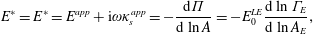 $$\begin{eqnarray}E^{\ast }=E^{\ast }=E^{app}+\text{i}\unicode[STIX]{x1D714}\unicode[STIX]{x1D705}_{s}^{app}=-\frac{\text{d}\unicode[STIX]{x1D6F1}}{\text{d}\ln A}=-E_{0}^{LE}\frac{\text{d}\ln \unicode[STIX]{x1D6E4}_{E}}{\text{d}\ln A_{E}},\end{eqnarray}$$
where
 $$\begin{eqnarray}E_{0}^{LE}=\frac{\text{d}\unicode[STIX]{x1D6F1}}{\text{d}\ln \unicode[STIX]{x1D6E4}_{E}}\end{eqnarray}$$
is the Marangoni modulus of the expanded phase. Substituting (5.12) in (5.14), the apparent surface dilatational elasticity and viscosity are
 $$\begin{eqnarray}E^{app}=E_{0}^{LE}\frac{1}{1+\unicode[STIX]{x1D701}_{p}^{2}},\quad \unicode[STIX]{x1D705}_{s}^{app}=\frac{E_{0}^{LE}}{\unicode[STIX]{x1D714}}\frac{\unicode[STIX]{x1D701}_{p}}{1+\unicode[STIX]{x1D701}_{p}^{2}}.\end{eqnarray}$$
Equation (5.16) has the form of a Maxwell fluid with a characteristic relaxation time scale $\unicode[STIX]{x1D70F}=k_{p}^{-1}$
, analogous to kinetic-limited adsorption of soluble surfactants (4.51).
$\unicode[STIX]{x1D70F}=k_{p}^{-1}$
, analogous to kinetic-limited adsorption of soluble surfactants (4.51).
Domains grow freely in the low-frequency limit ( $\unicode[STIX]{x1D714}\ll k_{p}$
or
$\unicode[STIX]{x1D714}\ll k_{p}$
or $\unicode[STIX]{x1D701}_{p}\gg 1$
) and the LE phase offers no resistance to compression (figure 28
a). By contrast, a finite and rate-dependent dilatational modulus emerges during the LE–LC coexistence when the compression rate and phase change rate are comparable, which derives from temporary compression of the LE ‘fluid’ before phase change has had a chance to occur. For surfactants with inherent surface viscosity (§ 3.4), measured surface dissipation must be interpreted as the appropriate combination of a true material property and apparent rate-dependent contributions due to phase changes and adsorption/desorption.
$\unicode[STIX]{x1D701}_{p}\gg 1$
) and the LE phase offers no resistance to compression (figure 28
a). By contrast, a finite and rate-dependent dilatational modulus emerges during the LE–LC coexistence when the compression rate and phase change rate are comparable, which derives from temporary compression of the LE ‘fluid’ before phase change has had a chance to occur. For surfactants with inherent surface viscosity (§ 3.4), measured surface dissipation must be interpreted as the appropriate combination of a true material property and apparent rate-dependent contributions due to phase changes and adsorption/desorption.
5.3 Non-constant surface viscosity
All discussion of surface rheology thus far has assumed surface shear and dilatational viscosities to be constant. However convenient this approximation may be, many factors can impart spatial, temporal and concentration-based heterogeneities to surface rheological properties. Phase transitions in Langmuir monolayers are typically accompanied by changes in surface-viscous and elastic properties. Liquid condensed domains can deform, reorient, jam or slip against each other in response to hydrodynamic forcing, leading to non-Newtonian behaviour. This nonlinear behaviour depends on the precise phase behaviour, which in turn varies based on surfactant type, hydrocarbon chain length, chain orientation and intermolecular interactions, as described in § 5.1. An exhaustive discussion on the resulting non-Newtonian behaviour is beyond the scope of this work, and we direct the reader to Fuller & Vermant (Reference Fuller and Vermant2012) and references within. Here, we will only provide a flavour of the richness and uniqueness of non-Newtonian surface rheology by outlining two examples – one with familiar 3-D analogues, and another which is almost never observed in three dimensions – both of which arise due to phase transitions in Langmuir monolayers.
5.3.1 Surface-shear thickening and thinning
Gradients in surface pressure drive flows along interfaces, just like bulk pressure gradients drive (Poiseuille) flows in pipes. For example, increasing the surface pressure on one end of an interfacial slit ‘pumps’ a monolayer through a 2-D channel, making a 2-D analogue of a syringe (Schwartz, Knobler & Bruinsma Reference Schwartz, Knobler and Bruinsma1994; Fuller & Vermant Reference Fuller and Vermant2012). Indeed, the subphase decouples from the interfacial stress balance (3.94) when interface-dominant ( $Bq=\unicode[STIX]{x1D702}_{s}/\unicode[STIX]{x1D702}R\gg 1$
), and the surface velocity
$Bq=\unicode[STIX]{x1D702}_{s}/\unicode[STIX]{x1D702}R\gg 1$
), and the surface velocity $u_{s}(y)$
of an incompressible monolayer obeys the familiar parabolic profile of Poiseuille flow in two dimensions
$u_{s}(y)$
of an incompressible monolayer obeys the familiar parabolic profile of Poiseuille flow in two dimensions
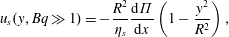 $$\begin{eqnarray}u_{s}(y,Bq\gg 1)=-\frac{R^{2}}{\unicode[STIX]{x1D702}_{s}}\frac{\text{d}\unicode[STIX]{x1D6F1}}{\text{d}x}\left(1-\frac{y^{2}}{R^{2}}\right),\end{eqnarray}$$
where $R$
the slit half-width (figure 29
a).
$R$
the slit half-width (figure 29
a).
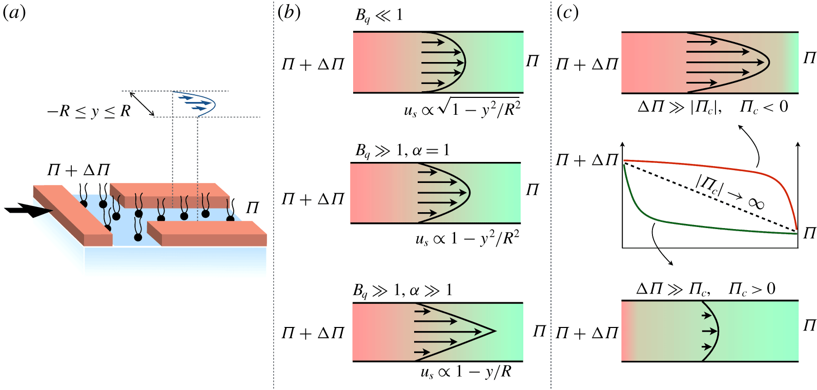
Figure 29. (a) A surface pressure gradient across an interfacial channel sets up a surface (and bulk) flow, much pressure-driven flow in three dimensions. (b) Illustrations of surface velocity profiles, with $\unicode[STIX]{x1D6FC}$
defined in (5.19):
$\unicode[STIX]{x1D6FC}$
defined in (5.19): $u_{s}(y)$
is elliptic when subphase dominant (
$u_{s}(y)$
is elliptic when subphase dominant ( $Bq\ll 1$
) and parabolic when interface dominant (
$Bq\ll 1$
) and parabolic when interface dominant ( $Bq\gg 1$
) with Newtonian surface rheology. However, condensed arachidic acid above
$Bq\gg 1$
) with Newtonian surface rheology. However, condensed arachidic acid above $\unicode[STIX]{x1D6F1}\sim 20~\text{mN}~\text{m}^{-1}$
surface shear thickens, resulting in triangular velocity profiles (5.19). The background colour gradient represents
$\unicode[STIX]{x1D6F1}\sim 20~\text{mN}~\text{m}^{-1}$
surface shear thickens, resulting in triangular velocity profiles (5.19). The background colour gradient represents $\unicode[STIX]{x1D6F1}(x)$
, which changes linearly across the length of the channel. (c) Surface pressure distribution in the channel is nonlinear when
$\unicode[STIX]{x1D6F1}(x)$
, which changes linearly across the length of the channel. (c) Surface pressure distribution in the channel is nonlinear when $\unicode[STIX]{x1D702}_{s}$
is a function of
$\unicode[STIX]{x1D702}_{s}$
is a function of $\unicode[STIX]{x1D6F1}$
. When
$\unicode[STIX]{x1D6F1}$
. When $\unicode[STIX]{x1D6F1}$
-thinning, surface pressure remains of the order of the driving pressure
$\unicode[STIX]{x1D6F1}$
-thinning, surface pressure remains of the order of the driving pressure $\unicode[STIX]{x0394}\unicode[STIX]{x1D6F1}$
for the majority of the channel and thus pumps a larger surfactant flux, effectively increasing the permeability of the channel. By contrast, surface pressure drops rapidly at the channel entrance when
$\unicode[STIX]{x0394}\unicode[STIX]{x1D6F1}$
for the majority of the channel and thus pumps a larger surfactant flux, effectively increasing the permeability of the channel. By contrast, surface pressure drops rapidly at the channel entrance when $\unicode[STIX]{x1D6F1}$
-thickening, which maintains a relatively small gradient across the rest of the channel, thereby ‘choking’ the surface flow.
$\unicode[STIX]{x1D6F1}$
-thickening, which maintains a relatively small gradient across the rest of the channel, thereby ‘choking’ the surface flow.
However, viscous coupling with the subphase modifies the surface flow from (5.17). When subphase dominant ( $Bq\ll 1$
), the solution to the incompressible Boussinesq–Scriven equation (3.94) is (Stone Reference Stone1995)
$Bq\ll 1$
), the solution to the incompressible Boussinesq–Scriven equation (3.94) is (Stone Reference Stone1995)
 $$\begin{eqnarray}u_{s}(y,Bq\ll 1)=-\frac{R}{\unicode[STIX]{x1D702}}\frac{\text{d}\unicode[STIX]{x1D6F1}}{\text{d}x}\sqrt{1-\frac{y^{2}}{R^{2}}}.\end{eqnarray}$$
Subphase-dominant flow (5.18) is insensitive to $\unicode[STIX]{x1D702}_{s}$
, and the flow profile is elliptic rather than parabolic, consistent with direct observation of Langmuir monolayers of negligible surface shear viscosity (Schwartz et al.
Reference Schwartz, Knobler and Bruinsma1994).
$\unicode[STIX]{x1D702}_{s}$
, and the flow profile is elliptic rather than parabolic, consistent with direct observation of Langmuir monolayers of negligible surface shear viscosity (Schwartz et al.
Reference Schwartz, Knobler and Bruinsma1994).
Increasing the surface shear viscosity – e.g. by compressing the monolayer so that rheologically stiff domains nucleate – transitions the surface velocity from (5.18) to (5.17). However, direct observation of the velocity profiles of heterogeneous arachidic acid monolayers by Kurnaz & Schwartz (Reference Kurnaz and Schwartz1997) reveals a non-Newtonian viscous response (figure 29 b). The velocity profile is shear-rate-dependent at sufficiently large flow rates, and approximately fits
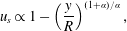 $$\begin{eqnarray}u_{s}\propto 1-\left(\frac{y}{R}\right)^{(1+\unicode[STIX]{x1D6FC})/\unicode[STIX]{x1D6FC}},\end{eqnarray}$$
with $\unicode[STIX]{x1D6FC}>1$
when surface-shear thickening, and
$\unicode[STIX]{x1D6FC}>1$
when surface-shear thickening, and $0<\unicode[STIX]{x1D6FC}<1$
when surface-shear thinning.
$0<\unicode[STIX]{x1D6FC}<1$
when surface-shear thinning.
Kurnaz & Schwartz (Reference Kurnaz and Schwartz1997) observed shear thinning in arachidic acid monolayers at high shear rates ( ${\gtrsim}0.1~\text{s}^{-1}$
) and low surface pressures, but shear thickening at higher
${\gtrsim}0.1~\text{s}^{-1}$
) and low surface pressures, but shear thickening at higher $\unicode[STIX]{x1D6F1}$
. The transition between the two occurs around
$\unicode[STIX]{x1D6F1}$
. The transition between the two occurs around $\unicode[STIX]{x1D6F1}\approx 20~\text{mN}~\text{m}^{-1}$
, where arachidic acid undergoes a tail group tilt–untilt transition (Kaganer et al.
Reference Kaganer, Möhwald and Dutta1999). This phase transition is associated with changes in surface rheology (Kurtz et al.
Reference Kurtz, Lange and Fuller2006; Zell et al.
Reference Zell, Nowbahar, Mansard, Leal, Deshmukh, Mecca, Tucker and Squires2014), suggesting that surfactant phase behaviour is at least in part responsible for the non-Newtonian dynamics. Other classes of surfactants show rate-dependent rheology upon phase transition as well; e.g. power-law models capture experimentally measured surface-shear thinning of DPPC at high surface pressures (Raghunandan et al.
Reference Raghunandan, Hirsa, Underhill and Lopez2018).
$\unicode[STIX]{x1D6F1}\approx 20~\text{mN}~\text{m}^{-1}$
, where arachidic acid undergoes a tail group tilt–untilt transition (Kaganer et al.
Reference Kaganer, Möhwald and Dutta1999). This phase transition is associated with changes in surface rheology (Kurtz et al.
Reference Kurtz, Lange and Fuller2006; Zell et al.
Reference Zell, Nowbahar, Mansard, Leal, Deshmukh, Mecca, Tucker and Squires2014), suggesting that surfactant phase behaviour is at least in part responsible for the non-Newtonian dynamics. Other classes of surfactants show rate-dependent rheology upon phase transition as well; e.g. power-law models capture experimentally measured surface-shear thinning of DPPC at high surface pressures (Raghunandan et al.
Reference Raghunandan, Hirsa, Underhill and Lopez2018).
5.3.2 The
$\unicode[STIX]{x1D6F1}$
-dependent viscosity

Surface viscosities of Langmuir monolayers change appreciably over surface pressure variations accessible in typical experiments. For instance, the surface shear viscosity of DPPC grows exponentially when $\unicode[STIX]{x1D6F1}$
is increased from
$\unicode[STIX]{x1D6F1}$
is increased from $5$
to
$5$
to $15~\text{mN}~\text{m}^{-1}$
(Kim et al.
Reference Kim, Choi, Zasadzinski and Squires2011, Reference Kim, Choi, Zell, Squires and Zasadzinski2013; Fuller & Vermant Reference Fuller and Vermant2012; Hermans & Vermant Reference Hermans and Vermant2014), unlike 3-D liquids which show such changes only under truly extreme pressures. The exponential dependence of surface viscosity on surface pressure can be understood in terms of the free-area analogue of classical free-volume theories of viscosity (Kim et al.
Reference Kim, Choi, Zell, Squires and Zasadzinski2013), and can be written as
$15~\text{mN}~\text{m}^{-1}$
(Kim et al.
Reference Kim, Choi, Zasadzinski and Squires2011, Reference Kim, Choi, Zell, Squires and Zasadzinski2013; Fuller & Vermant Reference Fuller and Vermant2012; Hermans & Vermant Reference Hermans and Vermant2014), unlike 3-D liquids which show such changes only under truly extreme pressures. The exponential dependence of surface viscosity on surface pressure can be understood in terms of the free-area analogue of classical free-volume theories of viscosity (Kim et al.
Reference Kim, Choi, Zell, Squires and Zasadzinski2013), and can be written as
 $$\begin{eqnarray}\unicode[STIX]{x1D702}_{s}(\unicode[STIX]{x1D6F1})=\unicode[STIX]{x1D702}_{s}^{0}\text{e}^{(\unicode[STIX]{x1D6F1}-\unicode[STIX]{x1D6F1}_{0})/\unicode[STIX]{x1D6F1}_{c}},\end{eqnarray}$$
where $\unicode[STIX]{x1D6F1}_{c}$
is a characteristic surface pressure change required to appreciably change
$\unicode[STIX]{x1D6F1}_{c}$
is a characteristic surface pressure change required to appreciably change $\unicode[STIX]{x1D702}_{s}$
, and
$\unicode[STIX]{x1D702}_{s}$
, and $\unicode[STIX]{x1D702}_{s}^{0}$
is a reference viscosity at reference pressure
$\unicode[STIX]{x1D702}_{s}^{0}$
is a reference viscosity at reference pressure $\unicode[STIX]{x1D6F1}_{0}$
. DPPC is a ‘
$\unicode[STIX]{x1D6F1}_{0}$
. DPPC is a ‘ $\unicode[STIX]{x1D6F1}$
-thickening’ surfactant with
$\unicode[STIX]{x1D6F1}$
-thickening’ surfactant with $\unicode[STIX]{x1D6F1}_{c}\approx 8~\text{mN}~\text{m}^{-1}$
, whereas setting
$\unicode[STIX]{x1D6F1}_{c}\approx 8~\text{mN}~\text{m}^{-1}$
, whereas setting $\unicode[STIX]{x1D6F1}_{c}\rightarrow \infty$
in (5.20) retrieves the Newtonian limit of constant
$\unicode[STIX]{x1D6F1}_{c}\rightarrow \infty$
in (5.20) retrieves the Newtonian limit of constant $\unicode[STIX]{x1D702}_{s}$
.
$\unicode[STIX]{x1D702}_{s}$
.
By contrast, the surface viscosity of some surfactants decreases with increasing surface pressure. For example, the surface viscosity of eicosanol (Kurtz et al.
Reference Kurtz, Lange and Fuller2006; Zell et al.
Reference Zell, Nowbahar, Mansard, Leal, Deshmukh, Mecca, Tucker and Squires2014) drops tenfold upon increasing $\unicode[STIX]{x1D6F1}$
from
$\unicode[STIX]{x1D6F1}$
from $10$
to
$10$
to $20~\text{mN}~\text{m}^{-1}$
as it undergoes a tilt–untilt transition (Kaganer et al.
Reference Kaganer, Möhwald and Dutta1999). Such ‘
$20~\text{mN}~\text{m}^{-1}$
as it undergoes a tilt–untilt transition (Kaganer et al.
Reference Kaganer, Möhwald and Dutta1999). Such ‘ $\unicode[STIX]{x1D6F1}$
-thinning’ behaviour can be modelled as in (5.20) by inverting the sign of
$\unicode[STIX]{x1D6F1}$
-thinning’ behaviour can be modelled as in (5.20) by inverting the sign of $\unicode[STIX]{x1D6F1}_{c}$
: for eicosanol,
$\unicode[STIX]{x1D6F1}_{c}$
: for eicosanol, $\unicode[STIX]{x1D6F1}_{c}\sim -3~\text{mN}~\text{m}^{-1}$
.
$\unicode[STIX]{x1D6F1}_{c}\sim -3~\text{mN}~\text{m}^{-1}$
.
The fact that $\unicode[STIX]{x1D702}_{s}$
can vary over orders of magnitude in rather mundane flows gives rise to qualitatively new flow phenomena. For example, flow through a thin gap (figure 29) amplifies surface pressure variations and therefore accentuate the
$\unicode[STIX]{x1D702}_{s}$
can vary over orders of magnitude in rather mundane flows gives rise to qualitatively new flow phenomena. For example, flow through a thin gap (figure 29) amplifies surface pressure variations and therefore accentuate the $\unicode[STIX]{x1D6F1}$
-dependent nature of
$\unicode[STIX]{x1D6F1}$
-dependent nature of $\unicode[STIX]{x1D702}_{s}$
. Using lubrication theory, the interface-dominant (
$\unicode[STIX]{x1D702}_{s}$
. Using lubrication theory, the interface-dominant ( $Bq\gg 1$
) incompressible Boussinesq–Scriven equation reduces to (Manikantan & Squires Reference Manikantan and Squires2017b
)
$Bq\gg 1$
) incompressible Boussinesq–Scriven equation reduces to (Manikantan & Squires Reference Manikantan and Squires2017b
)
 $$\begin{eqnarray}\frac{\unicode[STIX]{x2202}\unicode[STIX]{x1D6F1}}{\unicode[STIX]{x2202}x}=\unicode[STIX]{x1D702}_{s}(\unicode[STIX]{x1D6F1})\frac{\unicode[STIX]{x2202}^{2}u_{s}}{\unicode[STIX]{x2202}y^{2}}.\end{eqnarray}$$
Fortunately, (5.21) is solvable by separation despite the strong nonlinearity of $\unicode[STIX]{x1D702}_{s}$
, whether using the assumed form (5.20) or a measured
$\unicode[STIX]{x1D702}_{s}$
, whether using the assumed form (5.20) or a measured $\unicode[STIX]{x1D702}(\unicode[STIX]{x1D6F1})$
.
$\unicode[STIX]{x1D702}(\unicode[STIX]{x1D6F1})$
.
The impact of surface-pressure-dependent surface viscosity is best illustrated using the flux pumped through the channel. For a surface pressure gradient $\unicode[STIX]{x0394}\unicode[STIX]{x1D6F1}$
applied across a channel of length
$\unicode[STIX]{x0394}\unicode[STIX]{x1D6F1}$
applied across a channel of length $L\gg R$
, the interfacial flux
$L\gg R$
, the interfacial flux $Q$
is (Manikantan & Squires Reference Manikantan and Squires2017b
)
$Q$
is (Manikantan & Squires Reference Manikantan and Squires2017b
)
 $$\begin{eqnarray}Q=\frac{2}{3}\frac{\unicode[STIX]{x1D6F1}_{c}R^{3}}{\unicode[STIX]{x1D702}_{s}^{0}L}(1-\text{e}^{-\unicode[STIX]{x0394}\unicode[STIX]{x1D6F1}/\unicode[STIX]{x1D6F1}_{c}}).\end{eqnarray}$$
The familiar Newtonian flux is recovered when $\unicode[STIX]{x1D6F1}_{c}\gg \unicode[STIX]{x0394}\unicode[STIX]{x1D6F1}$
 $$\begin{eqnarray}Q(\unicode[STIX]{x0394}\unicode[STIX]{x1D6F1}\ll \unicode[STIX]{x1D6F1}_{c})\rightarrow Q_{Newt}=\frac{2}{3}\frac{\unicode[STIX]{x0394}\unicode[STIX]{x1D6F1}R^{3}}{\unicode[STIX]{x1D702}_{s}^{0}L}.\end{eqnarray}$$
Qualitative differences arise when $\unicode[STIX]{x0394}\unicode[STIX]{x1D6F1}$
is comparable to
$\unicode[STIX]{x0394}\unicode[STIX]{x1D6F1}$
is comparable to $\unicode[STIX]{x1D6F1}_{c}$
. Indeed,
$\unicode[STIX]{x1D6F1}_{c}$
. Indeed, $Q$
approaches a limiting value when
$Q$
approaches a limiting value when $\unicode[STIX]{x0394}\unicode[STIX]{x1D6F1}\gg \unicode[STIX]{x1D6F1}_{c}$
for a
$\unicode[STIX]{x0394}\unicode[STIX]{x1D6F1}\gg \unicode[STIX]{x1D6F1}_{c}$
for a $\unicode[STIX]{x1D6F1}$
-thickening surfactant (
$\unicode[STIX]{x1D6F1}$
-thickening surfactant ( $\unicode[STIX]{x1D6F1}_{c}>0$
)
$\unicode[STIX]{x1D6F1}_{c}>0$
)
 $$\begin{eqnarray}Q(\unicode[STIX]{x0394}\unicode[STIX]{x1D6F1}\gg \unicode[STIX]{x1D6F1}_{c})\rightarrow Q_{max}=\frac{2}{3}\frac{\unicode[STIX]{x1D6F1}_{c}R^{3}}{\unicode[STIX]{x1D702}_{s}^{0}L},\end{eqnarray}$$
which is insensitive to $\unicode[STIX]{x0394}\unicode[STIX]{x1D6F1}$
, with
$\unicode[STIX]{x0394}\unicode[STIX]{x1D6F1}$
, with $\unicode[STIX]{x1D6F1}_{c}$
effectively setting the surface pressure scale beyond which the channel is ‘choked’. When
$\unicode[STIX]{x1D6F1}_{c}$
effectively setting the surface pressure scale beyond which the channel is ‘choked’. When $\unicode[STIX]{x0394}\unicode[STIX]{x1D6F1}\gg \unicode[STIX]{x1D6F1}_{c}$
, the surface pressure drops rapidly near the entrance of the channel, where the surface viscosity is extremely high. The pressure in the rest of the channel remains of the order of
$\unicode[STIX]{x0394}\unicode[STIX]{x1D6F1}\gg \unicode[STIX]{x1D6F1}_{c}$
, the surface pressure drops rapidly near the entrance of the channel, where the surface viscosity is extremely high. The pressure in the rest of the channel remains of the order of $\unicode[STIX]{x1D6F1}_{c}$
, setting the scale for the maximum flux that may be pumped through the channel.
$\unicode[STIX]{x1D6F1}_{c}$
, setting the scale for the maximum flux that may be pumped through the channel.
Similarly, $Q$
grows exponentially with applied surface pressure difference when
$Q$
grows exponentially with applied surface pressure difference when $\unicode[STIX]{x0394}\unicode[STIX]{x1D6F1}\gg |\unicode[STIX]{x1D6F1}_{c}|$
for a
$\unicode[STIX]{x0394}\unicode[STIX]{x1D6F1}\gg |\unicode[STIX]{x1D6F1}_{c}|$
for a $\unicode[STIX]{x1D6F1}$
-thinning surfactant (
$\unicode[STIX]{x1D6F1}$
-thinning surfactant ( $\unicode[STIX]{x1D6F1}_{c}<0$
). For large
$\unicode[STIX]{x1D6F1}_{c}<0$
). For large $\unicode[STIX]{x0394}\unicode[STIX]{x1D6F1}$
, therefore,
$\unicode[STIX]{x0394}\unicode[STIX]{x1D6F1}$
, therefore, $\unicode[STIX]{x1D6F1}$
-thinning increases channel ‘permeability’. Indeed, some surfactants (e.g. arachidic acid) might simultaneously shear thicken and
$\unicode[STIX]{x1D6F1}$
-thinning increases channel ‘permeability’. Indeed, some surfactants (e.g. arachidic acid) might simultaneously shear thicken and $\unicode[STIX]{x1D6F1}$
-thin, so that the monolayer may be more permeable through an interfacial slit than is expected for traditional shear-thickening materials (Kurnaz & Schwartz Reference Kurnaz and Schwartz1997).
$\unicode[STIX]{x1D6F1}$
-thin, so that the monolayer may be more permeable through an interfacial slit than is expected for traditional shear-thickening materials (Kurnaz & Schwartz Reference Kurnaz and Schwartz1997).
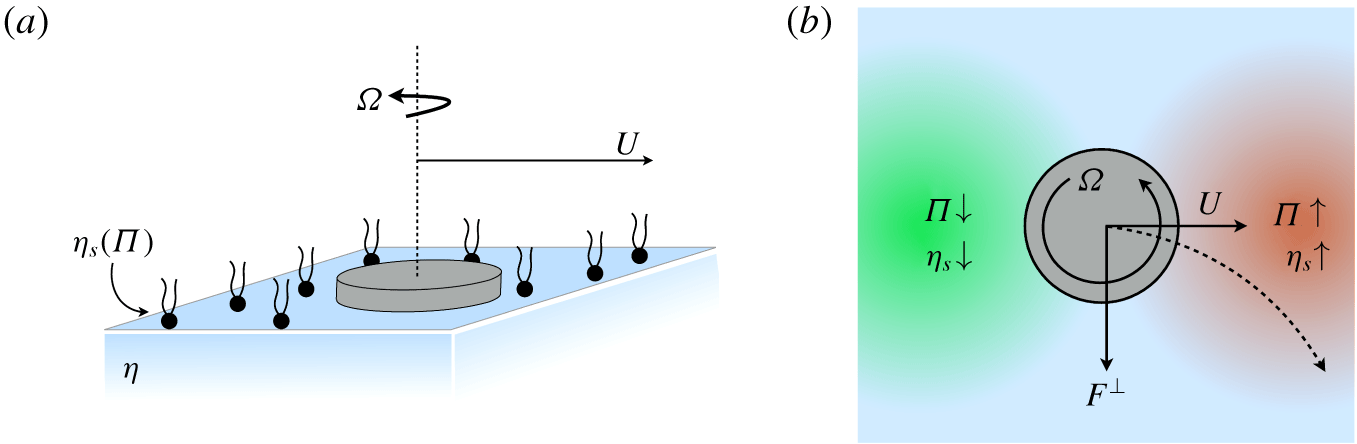
Figure 30. Surface ‘Magnus’ effect. (a) A circular particle forced to rotate while translating in a $\unicode[STIX]{x1D6F1}$
-thickening surfactant follows a Magnus-like trajectory (b) Surfactant in front of the translating disk has higher surface viscosity than the surfactant behind the disk, owing to the higher surface pressure. Consequently, the rotation of the particle causes it to ‘roll’ upwards, perpendicular to the direction of forcing (Manikantan & Squires Reference Manikantan and Squires2017a
).
$\unicode[STIX]{x1D6F1}$
-thickening surfactant follows a Magnus-like trajectory (b) Surfactant in front of the translating disk has higher surface viscosity than the surfactant behind the disk, owing to the higher surface pressure. Consequently, the rotation of the particle causes it to ‘roll’ upwards, perpendicular to the direction of forcing (Manikantan & Squires Reference Manikantan and Squires2017a
).
While thin gaps naturally give rise to large surface pressures and are easier to approach analytically, the consequences of $\unicode[STIX]{x1D6F1}$
-dependent
$\unicode[STIX]{x1D6F1}$
-dependent $\unicode[STIX]{x1D702}_{s}$
are not restricted to lubrication flows (Manikantan & Squires Reference Manikantan and Squires2017a
). For example, a disk translating while rotating on an unbounded and otherwise undisturbed
$\unicode[STIX]{x1D702}_{s}$
are not restricted to lubrication flows (Manikantan & Squires Reference Manikantan and Squires2017a
). For example, a disk translating while rotating on an unbounded and otherwise undisturbed $\unicode[STIX]{x1D6F1}$
-thickening/thinning monolayer experiences a force perpendicular to the direction of motion, analogous to the 3-D Magnus effect (figure 30), breaking the reversibility expected from Stokes flows. More generally,
$\unicode[STIX]{x1D6F1}$
-thickening/thinning monolayer experiences a force perpendicular to the direction of motion, analogous to the 3-D Magnus effect (figure 30), breaking the reversibility expected from Stokes flows. More generally, $\unicode[STIX]{x1D6F1}$
-dependent surface viscosities result in non-intuitive and kinematically irreversible trajectories of pairs of particles on the interface, which could lead to hydrodynamic aggregation, separation, and ‘lane formation’.
$\unicode[STIX]{x1D6F1}$
-dependent surface viscosities result in non-intuitive and kinematically irreversible trajectories of pairs of particles on the interface, which could lead to hydrodynamic aggregation, separation, and ‘lane formation’.
6 Conclusion
However long this Perspective may seem, it has at most laid out an intellectual skeleton for the mechanics and dynamics of surfactants in fluid systems. We have omitted many complications and subtleties that impact many different fields of science, industry and life. Still, we hope to have helped bridge the gap between the fluid mechanics community and the surfactant communities in physical chemistry, colloid and interface science.
We close this perspective with a philosophical reflection on the admittedly loose analogy we drew between surfactants in fluid dynamical systems, and the ‘hidden variables’ that were desperately sought in the early decades of quantum mechanics. As fluid mechanicians, we do not often stop to appreciate how remarkable the Navier–Stokes equations have been in capturing flows from nanometres to thousands of kilometres (fifteen orders of magnitude!) In many cases – particularly in turbulent flows – the challenges in solving fluid mechanics problems relate to the actual challenges in the mechanics of solving those problems. More powerful computers, more efficient algorithms and more insightful approximations are sought to improve predictions, elucidate new mechanisms and design new technologies. The basic equations that need to be solved, however, are generally not in question.
Surfactants, by contrast, introduce something different to the study of fluid systems. Although surfactants generally do nothing to alter the Navier–Stokes equations that govern the bulk fluid, they do change the boundary conditions that constrain them – and in so doing, completely change both the quantitative and qualitative aspects of the flow. As should be evident from this Perspective, any particular change in the observed dynamics might be caused by any of a number of distinct surfactant processes. Moreover, the ‘invisible’ nature of surfactants makes it difficult to know a priori what the surfactant is actually doing. This lands the typical fluid mechanician in unfamiliar terrain – of needing to determine what equations and boundary conditions must be solved in order to understand a fluid system, and ultimately predict its behaviour. We hope that our Perspective will help provide a conceptual map for this endeavour.
Finally, we close by noting that surfactants are by no means the only ‘hidden variables’ in fluid systems. So-called ‘complex fluids’ impact almost every industry and every aspect of life: shampoos and toothpastes, eggs and espressos, blood and mucous, paints, vaccines, lubricants and drilling muds. These natural and ‘formulated’ products generally contain a multitude of ingredients – liquids, solutes, surfactants, colloids and polymers – that impart mesostructures of various length scales, and affect the dynamic response properties on a variety of time scales. Still, these materials often appear homogeneous when viewed macroscopically. To understand, design and model the dynamics of these systems, one must identify and incorporate the additional concentration and stress fields associated with each component. And – just like with surfactants – one must often determine the actual equations that govern these additional components. The challenges are both rich and rewarding, and offer fertile ground for the curious fluid mechanician.
Acknowledgements
We gratefully acknowledge support from the National Science Foundation (NSF) under grant no. CBET-1512833 for support of this work, and from the National Heart, Lung, and Blood Institute of the National Institutes of Health under grant number R01HL135065. The content is solely the responsibility of the authors and does not necessarily represent the official views of the National Institutes of Health or the National Science Foundation. We gratefully acknowledge H. Stone for his particularly thorough and critical reading, insight and suggestions, and L. Walker for sharing her expertise, her insightful critiques and valuable perspective. We are grateful to I. Williams, G. Elfring, A. Khair, P. Linden and J. Zasadzinski for critical reading, comments and discussions, and to I. Williams for the unpublished image in figure 25(d).
Declaration of interests
The authors report no conflict of interest.


 Open access