

I. INTRODUCTION
The convolution neural network (CNN) offers excellent object classification performance due to its superior feature representation capability. This is automatically obtained by the backpropagation training process with a large amount of training data. Great efforts have been exerted to analyze the trained filters in order to explain CNN's performance. Existing visualization methods [Reference Mahendran and Vedaldi1–Reference Zeiler and Fergus3] reconstruct input images or visualize the responses to provide insights into the mechanism behind the activation of certain filters. Despite partial success in explaining CNN's performance, such analysis is less scalable given an increasing number of object classes and deeper network structures. In [Reference Agrawal, Girshick and Malik4], the average precision (AP) of an individual filter is computed and used as a quantitative measure of a trained CNN filter's discriminative ability. An important contribution of their work is to confirm the existence of ‘GMC-like features’.
Human brain cells that only respond to specific and complex visual stimuli (such as the face of one's grandmother) are called the grandmother cells (GMC) [Reference Quiroga, Reddy, Kreiman, Koch and Fried5]. They have been studied in artificial neural networks and are believed to play a critical role in object recognition. For example, the cat filter was extensively studied in [Reference Le6] for its resemblance to the cat-face GMC. The term ‘GMC-like features’ is used to refer to features or feature groups that respond solely to one object class. A similar concept is adopted in the standard feature encoding for image classification [Reference Hu, Deng and Guo7,Reference Wersing and Korner8].
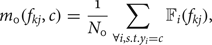
In Fig. 1, two conv_5 filters from the CaffeNet are used to demonstrate the importance of studying the GMC-like features. From left to right, the filters correspond to the ‘dining table’ and ‘dog’ object class, respectively. In the left, no dining table image is among the top nine activations and there is a significant overlap in the Gaussian confusion plot between the filter responses of the dining table and non-dining table classes. In the right, all top nine activations are dog images and there is little overlap in the Gaussian confusion plot between the filter responses of the dog and non-dog classes. The visual inspection of the top nine activations in Fig. 1 demonstrates the superior discriminative ability of GMC-like features, but such inspection cannot be conducted in large-scale networks due to the infeasible workload on the human inspector. Note that the Gaussian confusion plot reflects the important message of the top nine activations and, therefore, motivates us to develop the Gaussian confusion measure (GCM, see Section A), which yields a score representing the discriminative ability of a feature without human intervention.
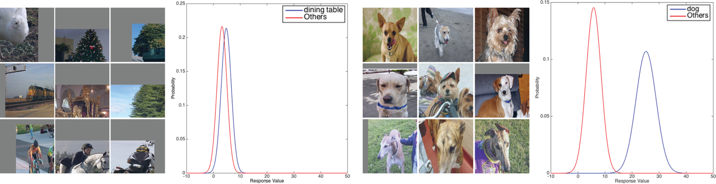
Fig. 1. None-GMC-like and GMC-like features are compared in the left and right subfigures. The first and third subfigures give the top nine activations for two conv5 filters and the second and fourth subfigures show their Gaussian confusion plot, which reflects the distribution of a filter's response value (see discussion in Section A). In this example, the GMC filter (i.e., filter 142 in conv5 of the fast-RCNN [Reference Girshick9] CaffeNet model) is mainly activated by the dog class and its Gaussian confusion plot shows better separation.
For certain object classes, one CNN feature is not a GMC-like feature by itself (see Section B). However, when a group of features work together, they behave as a GMC-like feature group. To understand the observation, we develop another measure called the cluster purity measure (CPM, see Section B) to gauge the group performance of features. As opposed to training an SVM for a subset of features and evaluating the resulting AP, CPM can be directly computed and not subject to the stochastic difference.
Our research goal is to gain a better understanding of the CNN by evaluating its trained features and studying the GMC-like features. It has three major contributions. First, we propose the GCM to automatically evaluate the performance of an individual filter. Second, we propose the CPM to automatically evaluate the group performance of a set of filters. They are both simple and efficient to train, and are useful in the automatic evaluation of the CNN features. Third, we study the CaffeNet and the VGG_M_1024 architectures by evaluating its filters using the proposed metrics. Our study provides an explanation of their stellar performance, reveals CNN's capability in detecting certain object (e.g. the dining table, see Section B), identifies potential issues with feature representations, and verifies the benefits of using deeper networks.
The rest of this paper is organized as follows. Related work is reviewed in Section II. Two metrics are introduced in Section III to evaluate whether a filter or a group of filters qualifies as the GMC-like feature. Experimental results based on the evaluation of the GMC-like features are reported in Section IV. Concluding remarks are provided in Section V.
II. RELATED WORK
A) GMC-like features
To better understand CNN trained features and their representations, several methods are proposed to find locally optimal visual inputs for individual filters in [Reference Zeiler and Fergus3,Reference Simonyan, Vedaldi and Zisserman10,Reference Yosinski, Clune, Nguyen, Fuchs and Lipson11]. Despite starting from different input priors, these methods were capable of selecting images that maximally activate a filter. By examining visualization results, one can verify the existence of GMC-like features as well as identify the targeted image content associated with the GMC-like feature. Besides visually inspecting features, Agrawal, et al. [Reference Agrawal, Girshick and Malik4] evaluated conv5 features with respect to their AP on the PASCAL-VOC 2012 dataset and showed the existence of GMC-like features for several object classes.
B) CNN interpretability
The exact purpose of filters in a convolution layer has been studied since early days of CNN research. It was observed in [Reference Girshick, Donahue, Darrell and Malik12,Reference Krizhevsky, Sutskever and Hinton13] that the conv1 features are low-level features such as edge, color, or texture. The deeper convolution layers extract higher-level features by assembling lower level features in the previous layer with different weights [Reference Li, Liu, Shen and van den Hengel14]. The pooling layers provide spatial and possibly rotation invariance to feature extraction [Reference Bengio, Goodfellow and Courville15]. The features assembly was studied in [Reference Srivastava, Masci, Gomez and Schmidhuber16]. It was concluded that only a local subnetwork is activated or trained for a specific input pattern. The selection is done through the local competition of several activation functions such as rectified linear, maxout and local winner-take-all. Research in [Reference Girshick, Iandola, Darrell and Malik17] reveals the CNN model structure by formulating the CNN as a deformable part model, where the convolution layers serve as part-feature detectors and the pooling layer uses a distance transform to assign different weight to part-detectors according to their relative locations. An interesting study conducted in [Reference Zhou, Khosla, Lapedriza, Oliva and Torralba18] indicates that object detectors could be trained to classify scene images, which have certain similarity as part-detectors are trained to recognize objects.
Kuo [Reference Kuo19] and [Reference Kuo20] studied the role of the nonlinear activation functions in CNNs. It was argued that the nonlinear activation units act as a rectifier and prevent the sign confusion problem. Without intermediate nonlinear activation units, a negative response at the first layer multiplied by a negative filter weight at the second layer produces the same sign as a positive response multiplied by a positive filter weight. The same confusion occurs between a negative response followed by a positive filter weight, and a positive response followed by a negative filter weight.
Additional insights can be obtained by investigating the vulnerability of CNNs. Adversarial examples [Reference Szegedy21] are generated by adding imperceptible perturbations to the original test image so that the neural network will make a different prediction. Goodfellow et al. [Reference Goodfellow, Shlens and Szegedy22] proposed a fast gradient sign method to efficiently compute perturbations. Xie et al. [Reference Xie, Wang, Zhang, Zhou, Xie and Yuille23] proposed a Dense Adversary Generation algorithm to generate adversarial examples for the semantic segmentation and object detection problems.
Zhang et al. [Reference Zhang, Wang and Zhu24] proposed a technique to detect representation bias of CNNs. Due to dataset bias, unrelated co-appearing features may be used by CNNs to estimate the target attribute. To detect such representation flaws, the method requires additional manual annotations on the attribute relationship. The attribute relationships encoded by CNNs are extracted and then compared with manually annotated relationships, where disagreements suggest flaws in representations.
Researchers also used interpretable graphs to encode knowledge from pretrained CNN. Zhang et al. [Reference Zhang, Cao, Shi, Wu and Zhu25] built a graph to find the knowledge hierarchy encoded by CNN conv-layers, where each node corresponds to a part. Zhang et al. [Reference Zhang, Yang, Wu and Zhu26] used the decision tree to obtain interpretable prediction rules of a trained network.
Some recent works aim to build interpretable alternatives to CNNs. Sabour et al. [Reference Sabour, Frosst and Hinton27] introduced the CapsNet using units named ‘capsules’ [Reference Hinton, Krizhevsky and Wang28]. They are groups of neurons. A capsule is implicitly associated with a visual entity. Instead of a scalar output, each capsule outputs a vector, whose orientation corresponds to certain properties (e.g., size and deformation) of the entity. The length of the vector encodes the probability of existence. The routing-by-agreement mechanism allows the model to build a hierarchical relationship between entities. Experiments on the MNIST [Reference LeCun, Cortes and Burges29] dataset showed that each dimension of the capsule output vector possessed semantic meanings such as width and stroke thickness. Chen et al. [Reference Chen, Duan, Houthooft, Schulman, Sutskever and Abbeel30] proposed a variant of the generative adversarial network (GAN) named the InfoGAN, which aims to obtain an interpretable representation in an unsupervised manner. It is achieved by maximizing the mutual information between a subset of input noise variables and the generated images. Experiments on the MNIST dataset [Reference LeCun, Cortes and Burges29], SVHN dataset [Reference Netzer, Wang, Coates, Bissacco, Wu and Ng31], 3D image datasets of faces [Reference Paysan, Knothe, Amberg, Romdhani and Vetter32] and chairs [Reference Aubry, Maturana, Efros, Russell and Sivic33] and CelebA face datasets showed that the subset of latent variables correspond to visual properties such as the digit width in the MNIST dataset, the lighting condition in the SVHN dataset, rotation in the 3D images, and the hair style in the celebA dataset.
C) Object detection networks
Since Girshick et al. [Reference Girshick, Donahue, Darrell and Malik12] introduced the RCNN to solve the object detection problem, many efforts have been done to improve its efficiency and accuracy. The spatial pyramid pooling (SPP) was proposed in [Reference He, Zhang, Ren and Sun34] to share convolution computations. Girshick [Reference Girshick9] added the bounding box regression and extended the finetuning to all layers for better accuracy. The time-consuming region proposal extraction was replaced by the region proposal network to speed up detection to near real-time in [Reference Ren, He, Girshick and Sun35]. Deeper network configurations [Reference Simonyan and Zisserman36,Reference Szegedy37] offered even better performance in the benchmarking datasets at the price of a higher training cost with more parameters. Although the performance can be further improved with larger networks, we are more interested in understanding the reason for their success. By understanding the strength and weakness of a network, it helps stretch the performance furthermore at a reasonable cost of added parameters.
III. EVALUATION METRICS
To train a CNN for object detection, each training sample contains an object in a region of interest (ROI) with class label c. The filter responses in convolution layers indicate trained features. In conv1, filters act as low-level feature extractors. As more information is aggregated in deeper convolution layers, filters become more discriminative and class-specific. As a result, filters will be activated by more specific inputs.
The problem of interest can be stated as follows. Given an ROI which has an object inside, we extract one value from the filter response at the conv5 layer by max pooling. There are 256 filters at the conv5 layer and, consequently, we obtain a response vector of dimension 256 for each input ROI. Our question is whether there exists one or a group of filters that can help separate an object class from other classes. In the following, we propose two metrics that offer a quantitative answer to this question.
A) Gaussian confusion measure
We use N testing data samples to test a CNN for a specific object class, say, class c. The testing samples consist of both positive ones that are in class c and negative ones that are not in class c. To analyze a specific filter, we take its response value from the 256-D response vector and collect N response values, each is associated with a class label. They can be classified into two groups according to their class labels; namely, in class c or not in class c. Consequently, we can draw two distribution curves of response values for the two groups. This explains the Gaussian confusion plots in Fig. 1, where the y-axis is the normalized histogram value and the x-axis is a specific filter response value. As shown in Fig. 1, each filter response can be well approximated by a Gaussian (or normal) function denoted by ℕ(m, σ), where m is the mean and σ is the standard deviation.
We can state the problem mathematically below. For a set of testing samples  $(\vec {x}_i, y_i)$, where $\vec {x}_i$ is the ROI and y i is the class label, we use ${\open F}_{i} (f_{kj})$ to denote the response value of f kj which is the jth filter in the kth convolution layer. We group the response values according to their class labels into ℂ groups, where ℂ is the number of class labels in the testing dataset.
To get the GCM from a given filter, f k j, and a given object class, c ∈ ℂ, we need to compute the mean and standard deviation of two hypotheses: H 0 and H 1, where H 0 states that the object belongs to class c while H 1 states that the object does not belong to class c. N 0 and N 1 indicate the number of objects belonging to the two hypotheses, respectively.
The mean and standard deviation of hypothesis H 0 can be computed as
 $$m_0 (f_{k j},c) = \displaystyle{1 \over N_0} \sum_{\forall i, s.t. y_i = c} {\open F}_{i}(f_{k j}),$$
 $$\sigma_0 (f_{k j},c) = \sqrt{\displaystyle{1 \over N_0} \sum_{\forall i, s.t. y_i = c} [{\open F}_{i}(f_{k j}) - m_0(f_{k j},c)]^2}.$$
The mean and standard deviation of hypothesis H 1 can be computed as
 $$m_1(f_{k j},c) = \displaystyle{1 \over N_1} \sum_{\forall i, s.t. y_i \ne c} {\open F}_{i}(f_{k j}),$$
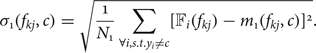 $$\sigma_1(f_{k j},c) = \sqrt{\displaystyle{1 \over N_1} \sum_{\forall i, s.t. y_i \ne c} [{\open F}_{i}(f_{k j}) - m_1(f_{k j},c)]^2}.$$
To decide whether a filter is activated, we should choose a threshold denoted by t. Then, the false positive is the probability of the Gaussian distribution ℕ(m 1, σ 1) falls in [t, + ∞). The false negative is the probability of the Gaussian distribution ℕ(m 0, σ 0) fall in ( − ∞, t]. The sum of these two error types can be written as:
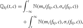 $$\eqalign{{\open Q}_{kj}(t,c) &= \int_{-\infty}^{t}{\open N}(m_0({f_{kj},c), \sigma_0(f_{kj},c})) \cr &\quad +\int_{t}^{\infty}{\open N}(m_1({f_{kj},c),\sigma_1(f_{kj},c})),}$$
It is typical to set
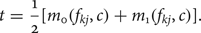 $$ t=\displaystyle{1 \over 2}[m_0(f_{kj},c)+m_1(f_{kj},c)]. $$
The specific object class that minimizes ℚkj(t, c) in equation (5) is a candidate class for us to search for its GMC response. Mathematically, we have
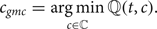 $$ c_{gmc} = \mathop{\hbox{argmin}}\limits_{c\in{\open C}} {\open Q}(t,c). $$
Finally, we define the GCM of filter f k j with respect to its corresponding c gmc as:
 $$ {\open GCM}(f_{k j}) = \displaystyle{{\open Q}_{kj}(t,c_{gmc}) \over {\open E}_j \{{\open Q}_{kj}(t,c_{gmc})\}} \Bigg{/} \displaystyle{m_0(f_{k j},c_{gmc})} {{\open E}_j\{m_0(f_{k j}, c_{gmc})\}}. $$
The numerator and the denominator of GCM in equation (8) are the normalized decision error and the normalized mean of the null hypothesis, respectively. Intuitively, a GMC-like feature should have a higher mean response, m 0(f kj, c), due to the higher correlation between objects of the same class. Besides, it should have a lower decision error ℚkj(t, c) since it can differentiate positive and negative samples at higher accuracy. As a result, GCM approaches 0 and a larger number for GMC-like and non-GMC-like features, respectively. This is supported by experimental results given in Fig. 2, where we show both the mean response value and the decision error of 256 conv5 features in a fast-RCNN trained CaffeNet with 40,000 iterations. Only three filters match the above description and the GCM successfully picks them out.

Fig. 2. The red and blue bars correspond to the decision error, ℚkj(t, c), and the null mean response, m 0(f kj, c), of the 256 conv5 filters of the fast-RCNN CaffeNet with 40,000 iterations, respectively. The blue bar is plotted bottom-up using the main vertical axis while the red bar is plotted top-down using the secondary vertical axis. The red dots indicate filters of indices 132, 178, and 205 (from left to right), which have the GCM score of 0.05, 0.9, and 0.17, respectively. These filter responses have low decision errors so that they are selected as GMC-like features. The top nine activations and the Gaussian confusion plot for each of these three cases are presented for validation.
The GCM provides an effective feature evaluation tool based on the statistics of the response values of a filter given different inputs. Its validity is verified via applying Gaussian tests to the response values extracted from Pascal [Reference Everingham, Van Gool, Williams, Winn and Zisserman38] dataset. It is also more thorough than evaluating the filter by APs since the GCM can model the underlining statistics of the filter (rather than testing the filter with a dataset). However, GCM is limited to the examination of a single filter. Thus, a new metric is needed for evaluating the group discriminative ability of a number of filters.
B) Cluster purity measurement
The CPM is proposed to evaluate how multiple filters perform jointly in differentiating object classes. As compared with the AP evaluation method introduced in [Reference Agrawal, Girshick and Malik4], the CPM metric does not require the separate training of an SVM.
To evaluate the CPM score on a set of n filters  $f_{k\vec {j}, \vec{j} \in {\open J}}$ in the kth convolution layer ( ${\open J}$ represents the set of filter indexes), the testing samples $(\vec {x_i},y_i)$ are organized into two groups, Ωc and $\Omega _{\not c}$. The first group contains testing samples belonging to class c while the second group contains testing samples not belonging to class c. In testing, the filter responses vector, $\vec{\open F}_i (f_{k\vec {j}})$, corresponding to the selected set of filters can be obtained at the convk layer. The responses vectors are n-dimensional vector. They can be split into two groups according to if the testing sample came from Ωc or $\Omega _{\not c}$. An example of the response vector in the 2D case is shown in Fig. 3.

Fig. 3. The response vectors of filter 188 (top left) and 212 (bottom left) in the 40000 iteration CaffeNet model are plotted in the 2D space. The blue dots in the plot corresponds to response vectors obtained from testing samples of cars and the red dots corresponds response vectors obtained from others. The plot in the right takes the top 200 responses vectors that are closest to the point P (shown as the star on the top right). The CPM score in this example is 0.87.
In operation, the CNN prefers a high response from a filter when it ‘fires’ on an input. The recent success in the Binary network [Reference Courbariaux, Bengio and David39] further proves the fact that most of CNN filter's behavior can be considered as an ON/OFF switch. This motivates the CPM metric for a set of filters that better discriminates a certain object class jointly. For this reason, we define a characteristic point at 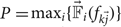 $P = \max\nolimits_i \{\vec{\open F}_i (f_{k \vec{j}})\}$ for an object class, where the max operation is taken over each dimension in the filter responses vector in the n-dimensional space.
As shown in Fig. 3, most points closer to P correspond to the ‘car’ testing samples. To quantitatively measure this property, we define the CPM metric as a measure of the percentage of points corresponding to the target object class within the top K closest points to point P. Mathematically, we have
 $${\open CPM}(\vec{\open F} (f_{k\vec{j}}), c) = \displaystyle{N_c \over K},$$
where N c is the number of responses vectors  $\vec{\open F}_i (f_{k \vec{j}})$, which are within the top K points closest to P, and correspond to testing samples with class label y i = c. We set K=200 empirically in the experiment.
In practice, we use the GCM metric to rank features' discriminative ability on each object class individually and, then, use the CPM metric to evaluate the joint discriminative ability of a selected group of features that perform well on a certain object class.
IV. EXPERIMENTAL RESULTS
We use the latest fast-RCNN [Reference Girshick9,Reference Jia40] implementation as the baseline. Since our objective is to analyze trained features, we disable the bounding box regression to avoid confusion. The analyzed network structure is the CaffeNet and VGG_M_1024, pretrained with the ImageNet CLS dataset [Reference Russakovsky41]. To visualize filter responses (i.e., features) and top activations, we use the deconv network [Reference Zeiler and Fergus3] and visualization toolbox from [Reference Yosinski, Clune, Nguyen, Fuchs and Lipson11]. Furthermore, deconv images and top nine activations are extracted separately using the PASCAL-VOC 2012 dataset with the whole image as the ROI. To save space, we also generate the 20 classes Gaussian confusion plot by combining all 20 individual Gaussian confusion plots.
A) Evaluating GMC features
Our experiment begins with applying the two developed metrics, GCM and CPM, to the conv5 features extracted from the CaffeNet. The fast-RCNN does not crop out ROIs until it reaches the fully connected layer. Thus, we created a new testing configuration, where the network ends at the ROI-pooling layer to obtain network responses at a given ROI. The ROI-pooling layer will output one maximum response value for each filter, which is used to evaluate whether the filter is activated or not. That is, for all 256 filters in the conv5 layer, we have a 256-D feature vector to denote the response of each of the filters.
A few examples of GMC and none-GMC like features are demonstrated in Fig. 4, where the top nine activations of the GMC-like features are all of the same object classes, and their GCM values indicate that these filters do not confuse other object classes. The activations of none-GMC-like features vary on the other hand. From left to right, filter 35 seems to look for the vertical line structure, filter 45 seems to look for the green color, filter 51 seems to look for the defocused background. Due to the space limit in the paper, the full filter GCM results are included in the supplemental material as the appendix.

Fig. 4. The red and blue bars correspond to the decision error, min cℚkj(t, c), and the null mean response value, m 0(f kj, c), of the 256 conv5 filters of the fast-RCNN CaffeNet with 40,000 iterations, respectively. (Note that these bars are different from those in Fig. 2, where ℚkj(t, c) and m 0(f kj, c) were plotted for c =“person”). The red bar is plotted top-down using the secondary vertical axis while the blue bar is plotted bottom-up using the main vertical axis. The red dots highlight filters 7, 132, and 246 from left to right. These filters have low decision errors and are selected as GMC-like features. The blue dots highlight filters 35, 45, and 51. These filters have higher decision errors and their responses are selected as none-GMC-like features. The top nine activations and their deconv results are presented to validate whether it is a GMC-like or none-GMC-like feature.
B) Evaluating GMC feature groups
Besides individual GMC-like features, the proposed CPM can find some interesting GMC-like feature groups. The top nine activations and the 20 classes Gaussian confusion plot of filter 188, 212, and 172 in conv5 are shown in Fig. 5.
Fig. 5. From left to right: the top nine activations and the 20 classes Gaussian confusion plot of filters 188, 212, and 172 in conv5 of the fast-RCNN CaffeNet with 40,000 iterations. The CPM score is 0.54 for filter 188 alone, 0.86 for filter 188 and filter 212 - it reaches 0.90 for the three filters group. The filters correspond to the tail, window, and head of the car, respectively.
The three filters are the top contributors of a feature group for the “car” object. Individually, each of them has a high decision error. They can get confused with different object classes (e.g., “bird” and “bus”). However, when the three work together, the discriminative power improves a lot and the feature group will mostly respond to the “car” images. As compared with an individual GMC, another advantage of the feature group is its robustness against occlusion. The GMC-like features are extremely sensitive to occlusion. This is a real issue in general object detection since objects are often partially occluded in images. Since the GMC-like feature group can respond to a subset of object's components, its detection performance will be more robust when an occlusion occurs.
C) Evaluating context features
Detection of a “dining table” and a “chair” is interesting as there is no clear definition of the object. Before applying the CNN to object detection, the APs of using the DPM [Reference Felzenszwalb, Girshick, McAllester and Ramanan42] in detecting a dining table and a chair are both low. They are 14.7 and 17.2%, respectively, in the PASCAL-VOC 2012 dataset [Reference Everingham, Van Gool, Williams, Winn and Zisserman38]. Recently, the fast-RCNN significantly boosts the corresponding performance to 40.7 and 67.9%. We observe from our experiment that the difference in the performance gain is due to “context features” trained by the network.
By identifying a group of features that corresponds to detecting “dining table” and plotting their top nine activations and the 20 classes Gaussian confusion plot in Fig. 6, we see that the key information used in detecting a dining table is cups and/or dishes placed on top of it. That is, while the DPM detector attempts to model the shape or contour of an object, there is little success in man-made objects due to intra-class variation. The CNN approaches this problem by summarizing the function of the dining table, which is to hold cups or dishes on top of it. This is quite close to how humans define a dining table: “an object to put dishes on”.
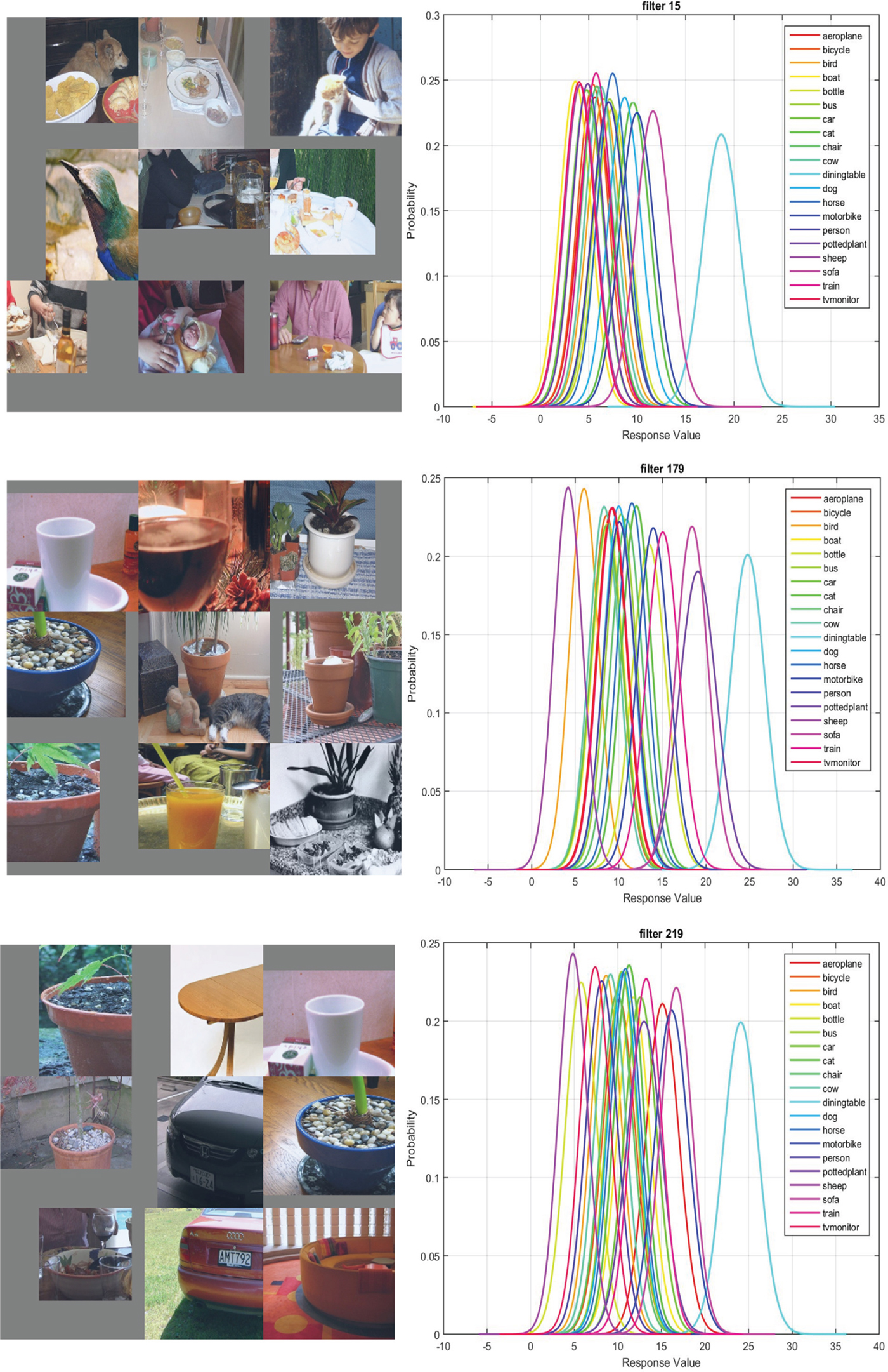
Fig. 6. From left to right: the top nine activations and the 20 classes Gaussian confusion plot of filters 16, 180, and 220 in conv5 of the fast-RCNN CaffeNet Model with 40,000 iterations. The CPM score is 0.36. These filters correspond to dishes, cups, an ellipse contour, respectively. Filters 16 and 180 are not related to a dining table itself but rather objects placed on top of it.
Besides context features that correspond to the function of an object, CNN also learns the context features that associate with the most probable background of an object. In Fig. 7, the three features have a CPM score of 0.61. However, the top nine activations and the 20 classes Gaussian confusion plot both confirm that the features are not learned to detect ‘airplanes’ but the background.
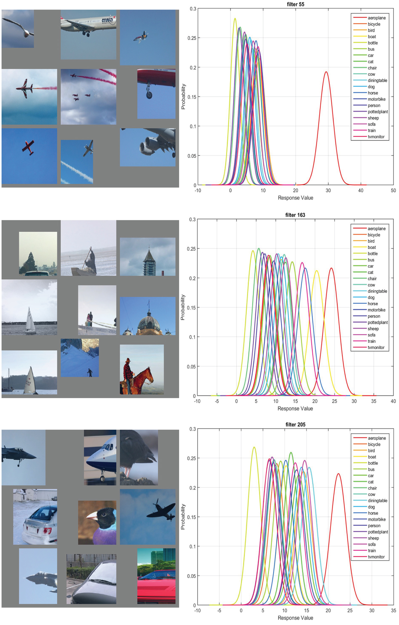
Fig. 7. The top nine activations and the 20 classes Gaussian confusion plot of filters 56, 164, and 206 in conv5 of the fast-RCNN CaffeNet Model with 40,000 iterations are shown from left to right. The CPM score is 0.61. These filters are all dedicated to detecting blue or gray color in the input, which are the typical background associated with “airplanes”.
D) Evaluating shared features
The CNN also learns shared features that have the superior discriminative ability over a few object classes. In Fig. 8, the top nine activations and the Gaussian confusion plot verify that the underlying feature tries to detect the wheel of a motorbike or a bicycle. Although the top nine activations include examples of the wheel of cars, the Gaussian confusion plot indicates that the filter is less capable of differentiating cars from others. As shown, the feature can differentiate motorbikes and bicycles from other objects, but cannot separate them well. This example demonstrates the first type of shared feature, which corresponds to certain shared characteristics across different object classes such as a common part of different objects.
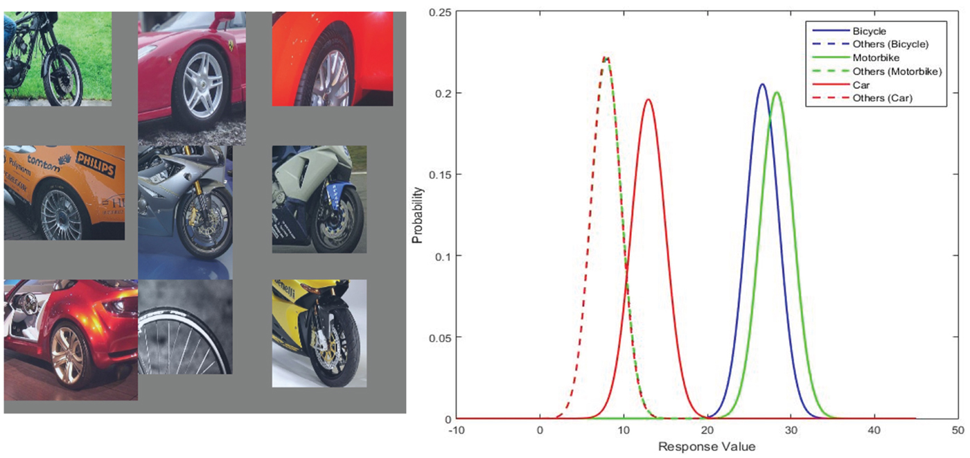
Fig. 8. From left to right: (1) the top nine activations of filter 216 in conv5 layer of the 40000 iteration CaffeNet model, and (2) the Gaussian confusion plot of the bicycle versus others, the motorbike versus others, and the car versus others.
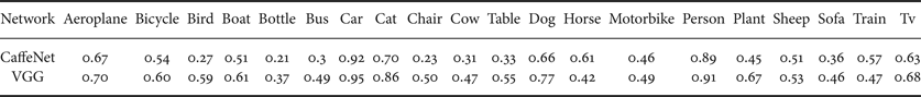
Table 1. The CPM scores of the top 5 features in the CaffeNet and the VGG_M_1024 for each object class.
There is another type of shared features, which not only corresponds to multiple object classes but has the discriminative ability to separate object classes. In Fig. 9, the top nine activations and the Gaussian confusion plot verify that the feature tries to detect the ear of cats, dogs or horses. Unlike the previous example, this feature has different response value ranges for the three object classes and can separate them with small decision errors. Since this feature's discriminative ability is closely related to the actual response values, it will be deprecated in the binary network [Reference Courbariaux, Bengio and David39]. This explains why the binary network could only achieve similar performance as the floating point network but could not outperform it.
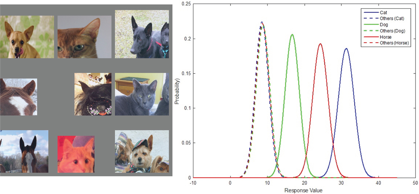
Fig. 9. From left to right: (1) the top nine activations of filter 141 in conv5 layer of the 40000 iteration CaffeNet model, and (2) the Gaussian confusion plot of the cat versus others, the horse versus others, and the dog versus others.
E) Other features
Besides the features that correspond to one or several object classes, the CNN learns features that seem to have little discriminative ability between classes. Usually, these features correspond to generic texture, shape or color. In Fig. 10, the top nine activations indicate that the filter is looking for mesh-like texture. The corresponding Gaussian confusion plot indicates that the feature can hardly differentiate between any classes by itself.
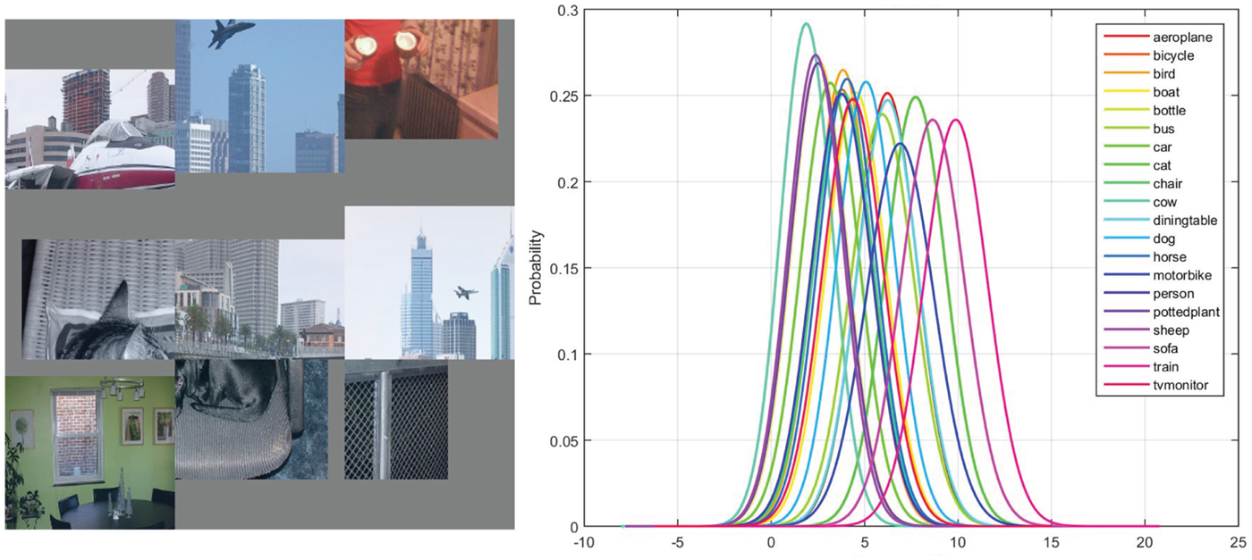
Fig. 10. From left to right: (1) the top nine activations of filter 214 in conv5 layer of the 40000 iteration CaffeNet model, and (2) the Gaussian confusion plot of all 20 object classes.
There is also another type of filter, which is confirmed to be an “unused” filter for classification. An example is shown in Fig. 11, where the top nine activations indicate that the filter is looking for parallel vertical patterns. However, the Gaussian confusion plot of all 20 object class shows that the feature has the same response range for all object classes. By examining the FC1 weight assigned to this conv5 feature, we see that it is almost ignored since the weight for this filter is negligible. Although these type of features seem to have little use in classification, they contribute strongly for generation tasks. The recent success in style transfer [Reference Gatys, Ecker and Bethge43] relies heavily on these generic features as they contribute to the computation of the “style loss”.
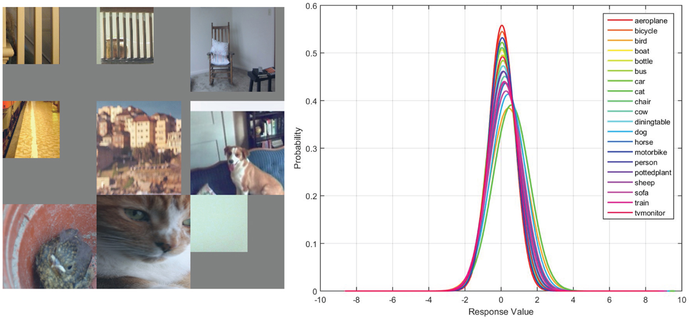
Fig. 11. From left to right: (1) the top nine activations of filter 35 in conv5 layer of the 40000 iteration CaffeNet model, and (2) the Gaussian confusion plot of all 20 object classes.
F) Comparison between VGG_M_1024 and CaffeNet
The VGG_M_1024 network structure used in the fast-RCNN benchmark is selected for comparison with the CaffeNet. The two networks start from the same 96 conv1 features, which are combined into 256 features in conv2. From that point on, while the CaffeNet has 384, 384, and 256 features in conv3, conv4, and conv5 layers, respectively, the VGG_M_1024 has 512, 512, and 512 features in its corresponding layers. The CaffeNet uses grouping to divide filters into two groups due to the GPU memory limit at their development time, which results in divided feature representation that may be less optimal as compared with VGG_M_1024 where all features are combined.
Due to the larger capacity in deeper convolution layers, the VGG_M_1024 model has a higher chance to learn GMC-like features, and the feature representation learned is more comprehensive and discriminative. An example is the “bottle” object class, where the CaffeNet has no GMC-like feature while the VGG_M_1024 have two GMC-like features. As shown in Figs 12 and 13, the most discriminative features trained by the CaffeNet are not GMC-like features. Thus, the decision error is large. In contrast, there are two GMC-like features trained by the VGG_M_1024, leading to low decision errors. In general, features trained from VGG_M_1024 tend to be more discriminative, and more GMC-like features can be found in VGG_M_1024. A summary of the feature representation for each object class is concluded in Table 1, where the CPM scores of the top 5 features for each object class are compared between the CaffeNet and the VGG_M_1024. The comparison further verifies that deeper networks learn better feature representation.

Fig. 12. The top three filters in the CaffeNet trained to detect the “bottle” object. Their corresponding Gaussian confusion plots are shown under the top nine activations.
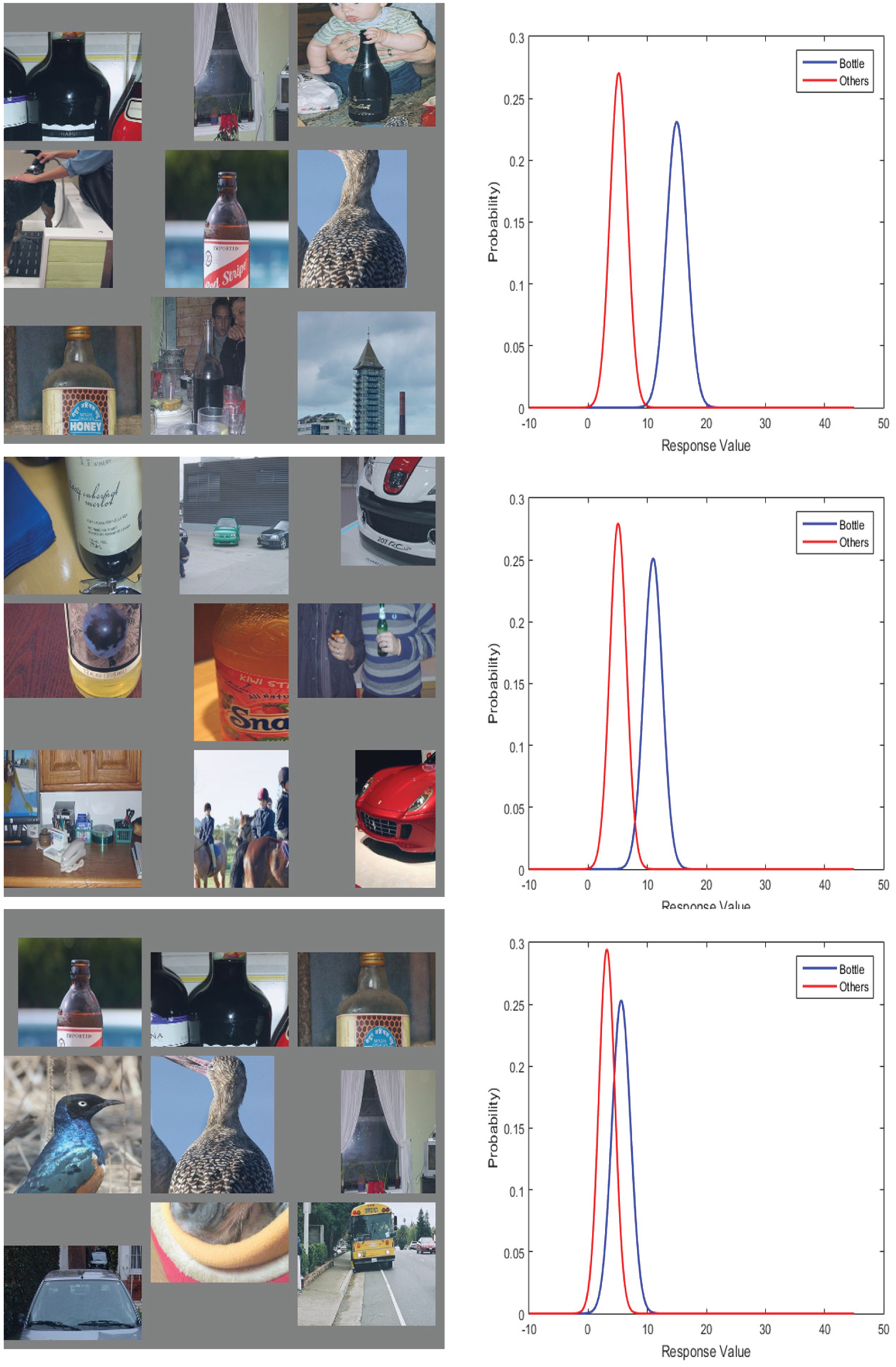
Fig. 13. The top three filters in the VGG_M_1024 (right) trained to detect the “bottle” object. Their corresponding Gaussian confusion plots are shown under the top nine activations.
G) Complete filter profile
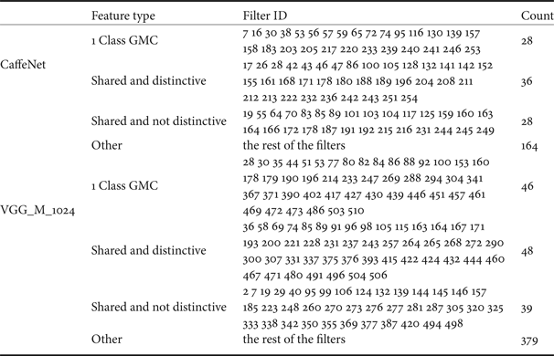
After analyzing the complete set of CNN trained features, we summarize different types of features trained by the CaffeNet and the VGG_M_1024 in Table 2, where the “1 class GMC” features correspond to features that differentiate one object class from the others (e.g., the dog example in Fig. 1), the “shared and distinctive” features correspond to features that differentiate several object classes from the others but cannot differentiate within these classes (e.g., example in Fig. 9), the “shared and not distinctive” feature correspond to features that differentiate several object classes from the others and differentiate within these classes (e.g., example in Fig. 8), and the ‘other’ features include the rest of the more generic features.
Table 2. The functionality summary of conv5 filters trained by the CaffeNet and the VGG_M_1024.
H) Summary
We have identified the following feature types learned by CNNs:
(i) GMC-like features or feature groups;
(ii) context features related to the function or most probable background of the object;
(iii) distinctive or non-distinctive shared features;
(iv) non-discriminant features.
We also verified that deeper networks can learn more GMC-like features so as to yield better performance.
V. CONCLUSION
Two effective metrics (i.e., GCM and CPM) to evaluate trained features of CNNs were proposed in this work. Thorough studies were conducted on deep features learned from the CaffeNet and VGG_M_1024 network based on these metrics. We identified different feature types, compared their discriminative ability, and analyzed the advantages of the deeper network structure in the experiment. Finally, we provided a full conv5 feature profile for both the CaffeNet and VGG_M_1024 to conclude our study.
Understanding CNN features can help understand what exactly has been learned in the network. Our study could potentially contribute to the development of automatic algorithms to determine the optimal network structure. It provides a quantitative evaluation of learned networks by introducing a loss term that is related to the CNN structure [Reference Liu44].
ACKNOWLEDGEMENT
Computation for the work described in this paper was supported by the University of Southern California's Center for High-Performance Computing (hpc.usc.edu).
Hao Xu received the B.S. in Electrical Engineering from Purdue University in 2010 and received his Ph.D. degree from University of Southern California in 2017. He joined Google after completing his Ph.D. studies. His research interest lies in 3D image/video rendering, 2D/3D video conversion, and Object Detection.
Yueru Chen is a Ph.D. student at University of Southern California. She received her Bachelor's degree in Physics from the University of Science and Technology of China, China in June 2014. Her research interests include 3D retrieval and computer vision.
Ruiyuan Lin is a Ph.D. student at University of Southern California. She received her Bachelor's degree in Information Engineering from City University of Hong Kong in July 2016. Her research interests include computer vision and machine learning.
C.-C. Jay Kuo received his Ph.D. degree from the Massachusetts Institute of Technology in 1987. He is now with the University of Southern California (USC) as Director of the Media Communications Laboratory and Dean's Professor in Electrical Engineering-Systems. His research interests are in the areas of digital media processing, compression, communication and networking technologies. Dr. Kuo is a Fellow of AAAS, IEEE and SPIE. He has guided 140 students to their Ph.D. degrees and supervised 25 postdoctoral research fellows. Dr. Kuo is a co-author of about 260 journal papers, 900 conference papers, 14 books and 30 patents. Dr. Kuo received the 1992 National Science Foundation Young Investigator (NYI) Award, the 1993 National Science Foundation Presidential Faculty Fellow (PFF) Award, the 2010 Electronic Imaging Scientist of the Year Award, the 2010-11 Fulbright-Nokia Distinguished Chair in Information and Communications Technologies, the 2014 USC Northrop Grumman Excellence in Teaching Award, the 2016 USC Associates Award for Excellence in Teaching, the 2016 IEEE Computer Society Taylor L. Booth Education Award, the 2016 IEEE Circuits and Systems Society John Choma Education Award, the 2016 IS&T Raymond C. Bowman Award, and the 2017 IEEE Leon K. Kirchmayer Graduate Teaching Award.


 Open access