


INTRODUCTION
The ideal source material for radiocarbon (14C) calibration is wood which has a calendar age determined by dendrochronology. There is, however, no immediate prospect for this to cover the full range of the radiocarbon dating technique and so we must therefore fall back on other types of record for the older section of the curve, all of which have their strengths and limitations. The five key types of record are:
Marine corals directly dated by uranium series methods (such as Bard et al. Reference Bard, Arnold, Hamelin, Tisnerat-Laborde and Cabioch1998): these have the advantage of having a directly determined calendar age, but the disadvantage of a marine reservoir offset in their radiocarbon content compared to the atmosphere (which is potentially variable), and that they are unable to provide a continuous record as their survival is sporadic.
Marine sedimentary records (such as Hughen et al. Reference Hughen, Lehman, Southon, Overpeck, Marchal, Herring and Turnbull2004): these have the advantage of being continuous, but the disadvantage of a marine radiocarbon reservoir offset, and a reliance on a climatically tuned age model.
Speleothem records (in particular Cheng et al. Reference Cheng, Lawrence Edwards, Southon, Matsumoto, Feinberg, Sinha, Zhou, Li, Li and Xu2018): these are both continuous and can be directly dated by uranium series methods, but the disadvantage of a potentially variable dead-carbon contribution or a possible reservoir effect (see below).
Floating tree-ring records (for example Turney et al. Reference Turney, Palmer, Bronk Ramsey, Adolphi, Muscheler, Hughen, Staff, Jones, Thomas, Fogwill and Hogg2016): these are direct records of atmospheric radiocarbon, and continuous, but normally limited in duration. Their relative age control is good but their absolute age must be determined in relation to other records.
Terrestrial plant macrofossils from varved lake sediments (Bronk Ramsey et al. Reference Bronk Ramsey, Staff, Bryant, Brock, Kitagawa, van der Plicht, Schlolaut, Marshall, Brauer and Lamb2012): these have the advantage of being atmospheric (since the plant species sampled are not aquatic), can have very good relative age control and be quasi-continuous (depending on the frequency of macrofossil remains). Their disadvantages are that the varve chronologies have significant cumulative uncertainties, and finding enough substantial plant macrofossils can be a challenge.
In practice, these different strengths and weaknesses mean that it is best to use all of these types of record in the construction of a curve (see other papers in this volume).
This paper focuses on the combined strength gained by using lake sediments and speleothems. More specifically, we look particularly at the lacustrine sediment record of Lake Suigetsu, central Japan (Nakagawa et al. Reference Nakagawa, Gotanda, Haraguchi, Danhara, Yonenobu, Brauer, Yokoyama, Tada, Takemura and Staff2012) which is unusual in covering the full range of the radiocarbon technique, with varves (albeit of variable quality) throughout the period for which we have no dendrochronogically based calibration datasets. Furthermore, the record contains large numbers of substantial terrestrial plant macrofossils, radiocarbon dated by three different laboratories (Kitagawa and van der Plicht Reference Kitagawa and van der Plicht1998; Bronk Ramsey et al. Reference Bronk Ramsey, Staff, Bryant, Brock, Kitagawa, van der Plicht, Schlolaut, Marshall, Brauer and Lamb2012). We also choose to focus on the unique series of speleothem records from Hulu Cave, China (Southon et al. Reference Southon, Noronha, Cheng, Edwards and Wang2012; Cheng et al. Reference Cheng, Lawrence Edwards, Southon, Matsumoto, Feinberg, Sinha, Zhou, Li, Li and Xu2018) characterized by an unusually low dead carbon fraction or reservoir effect, and with coverage over the same range of the pre-Holocene period.
REVISED VARVE CHRONOLOGY
The 2018 Suigetsu varve chronology (SG062018 vyr BP chronology; Schlolaut et al. Reference Schlolaut, Staff, Brauer, Lamb, Marshall, Bronk Ramsey and Nakagawa2018) is based on the counts of seasonal layers using thin section microscopy. Compared to the 2012 varve chronology (SG062012 vyr BP chronology; Bronk Ramsey et al. Reference Bronk Ramsey, Staff, Bryant, Brock, Kitagawa, van der Plicht, Schlolaut, Marshall, Brauer and Lamb2012; Marshall et al. Reference Marshall, Schlolaut, Nakagawa, Lamb, Brauer, Staff, Bronk Ramsey, Tarasov, Gotanda, Haraguchi, Yokoyama, Yonenobu and Tada2012) the 2018 iteration has been extended by approximately 10 ka to a composite depth of 4041 cm (correlation model ver. 28 Feb. 2019). This depth marks a facies boundary and the onset of consistent seasonal layer occurrence. However, in on average 50% of the years above this point either seasonal layers did not form or were not preserved. These indistinguishable layers were interpolated using a new Varve Interpolation Program (VIP; Schlolaut et al. Reference Schlolaut, Staff, Brauer, Lamb, Marshall, Bronk Ramsey and Nakagawa2018). The use of the new program marks a major change to the previous 2012 varve chronology, as the new program uses an entirely different interpolation approach based on deriving varve thickness frequency distributions from the incomplete count dataset and using these for interpolation. Another major difference between the 2012 and 2018 varve chronologies is that data from a second, independent counting method using µXRF data (Marshall et al. Reference Marshall, Schlolaut, Nakagawa, Lamb, Brauer, Staff, Bronk Ramsey, Tarasov, Gotanda, Haraguchi, Yokoyama, Yonenobu and Tada2012), were not incorporated in the 2018 varve chronology. The main reason for this exclusion was that, due to a methodological limit, thin varves may be systematically underrepresented in intervals with a low sedimentation rate in the µXRF count. Whether and where this might be the case cannot be said with certainty. Thus the µXRF count data were only used for comparison with the microscope data, but not incorporated in the final result. Despite these major changes, the 2012 and 2018 varve chronologies are in very good agreement for most of the record, with a notable exception between 1980 and 2375 cm composite depth. In this interval the 2018 varve chronology suggests a higher sedimentation rate, i.e. younger ages, though the 2012 chronology is still within the error estimate of the 2018 chronology.
THE HULU SPELEOTHEM RECORD
The Hulu cave 14C record from Tang Shan, near Nanjing in Eastern China, consists of three speleothems (H82, Southon et al. Reference Southon, Noronha, Cheng, Edwards and Wang2012; MSD and MSL, Cheng et al. Reference Cheng, Lawrence Edwards, Southon, Matsumoto, Feinberg, Sinha, Zhou, Li, Li and Xu2018). Combined, these speleothems provide a long and high-resolution record of 14C measurements together with equally high-resolution precise U-Th dates that extend back to 54 ka cal BP. While, as described in the Introduction, all speleothems have a potentially time-varying dead carbon fraction, within the three Hulu cave speleothems this is believed to be particularly small and stable based on assessment of their overlap with dendrochronologically dated trees and one another.
Between 10.6 and 54 ka cal BP, the Hulu cave record consists of ~500 14C determinations with corresponding, independent calendar age estimates obtained predominantly from paired U-Th dates. We created a Hulu-cave-only (Hulu-Cal) estimate of atmospheric 14C using the same errors-in-variables Bayesian spline approach taken to create the main IntCal20 curve (see Heaton et al. Reference Heaton, Blaauw, Blackwell, Bronk Ramsey, Reimer and Scott2020 in this issue). The uncertainties on the U-Th based calendar ages for each 14C determination were considered independent from one another. Within each speleothem the dead carbon fraction was modelled to have varied independently by up to ±50 years (1 sigma) around its mean value from one determination to the next; and these three means were permitted to take slightly different levels in each speleothem (with priors taken from Southon et al. Reference Southon, Noronha, Cheng, Edwards and Wang2012 and Cheng et al. Reference Cheng, Lawrence Edwards, Southon, Matsumoto, Feinberg, Sinha, Zhou, Li, Li and Xu2018). As for the main IntCal20 curve, 400 knots were used for the spline basis, placed according to the density of the observed calendar ages to enable variable smoothing, and with an uninformative prior on the smoothing parameter. The tempered Markov Chain Monte Carlo (MCMC) algorithm was run for 250,000 iterations with the first half-discarded as burn-in.
PRELIMINARY TIMESCALE METHODOLOGY
In order to make use of the relative dating strength of varves, and the absolute dating precision of U-Th methods, we have set out to provide a revised preliminary calendar timescale for Lake Suigetsu core SG06. The approach taken here is to use the same methodology as applied by Bronk Ramsey et al. (Reference Bronk Ramsey, Staff, Bryant, Brock, Kitagawa, van der Plicht, Schlolaut, Marshall, Brauer and Lamb2012) but updated in the light of the newly interpolated and extended varve chronology (Schlolaut et al. Reference Schlolaut, Staff, Brauer, Lamb, Marshall, Bronk Ramsey and Nakagawa2018) and the availability of the combined Hulu speleothem timescale (Cheng et al. Reference Cheng, Lawrence Edwards, Southon, Matsumoto, Feinberg, Sinha, Zhou, Li, Li and Xu2018) covering the entire age range. The approach taken here is slightly simpler because the speleothem record now covers the entire age range, and the varve chronology now covers almost all of the relevant depth range within the SG06 Suigetsu core.
All of the dates within the SG06 composite depth range 1397.4–4040.75 cm were included in the analysis with the exception of SUERC-28223 which had a sufficiently high error that it was quoted as >42700 BP (entirely consistent with the other data but not useful). This constitutes 639 radiocarbon dates from both the SG93 (Kitagawa and van der Plicht Reference Kitagawa and van der Plicht1998) and SG06 (Bronk Ramsey et al. Reference Bronk Ramsey, Staff, Bryant, Brock, Kitagawa, van der Plicht, Schlolaut, Marshall, Brauer and Lamb2012) cores measured at the Groningen, Oxford and SUERC laboratories. This is possible because of cross-correlation between the cores (Staff et al. Reference Staff, Schlolaut, Ramsey, Brock, Bryant, Kitagawa, van der Plicht, Marshall, Brauer and Lamb2013). There are some duplicate measurements so the dates correspond to 593 distinct depths. Each of these depths has been assigned a varve age (SG062018 vyr BP), based on the new updated varve counts and interpolation method (Schlolaut et al. Reference Schlolaut, Staff, Brauer, Lamb, Marshall, Bronk Ramsey and Nakagawa2018), the mean estimate of which is used as the depth parameter in a Poisson-process model.
As described in the previous section, a comparison curve was compiled from the standalone Hulu dataset and used in place of a calibration curve. An OxCal Poisson-process P_Sequence model (Bronk Ramsey Reference Bronk Ramsey2008) was then run to produce an age-age model for SG06 against the Hulu timescale. The rigidity of the model was set with a k parameter of 0.2, for the reasons outlined in, and for consistency with, the modelling performed by Bronk Ramsey et al. (Reference Bronk Ramsey, Staff, Bryant, Brock, Kitagawa, van der Plicht, Schlolaut, Marshall, Brauer and Lamb2012). However, the sensitivity of the model to different choices of this parameter was investigated (at k=0.1, which is less rigid, and k=0.3, which is more rigid). The results of these tests are shown in Figure 1.

Figure 1 This shows the differences between the varve age model (Schlolaut et al. Reference Schlolaut, Staff, Brauer, Lamb, Marshall, Bronk Ramsey and Nakagawa2018) and preliminary age models based on both the varves and the Hulu timescale (Cheng et al. Reference Cheng, Lawrence Edwards, Southon, Matsumoto, Feinberg, Sinha, Zhou, Li, Li and Xu2018), as plotted against the varve chronology age (before AD 1950). The top panel shows offsets relative to the varve chronology: the grey band shows the 95% confidence range for the varve chronology and the red, green and blue bands show the offsets relative to the varve chronology with a 2-σ error margin using three different values of the k parameter within the P_Sequence model (see text; the value of k used for the preliminary timescale was 0.2. The lower panel shows the inferred number of varves (from the varve chronology) per year, based on the different models: a value lower than 1 implies an underestimation of the sedimentation rate in the interpolation result, and a value higher than 1 implies an overestimation (see Discussion). (Please see electronic version for color figures.)
Unlike the normal modelling situation, where we expect the modelling datasets and calibration curve to be in good agreement, here, we would expect there to be some systematic differences for the reasons discussed below. In practice there were many dates with significantly low agreement indices, so we also tested the impact of increasing the relative uncertainty in the radiocarbon dates between the Hulu and Suigetsu datasets by both 100 and 200 years. Although this did produce slightly different model outputs (particularly in the region <15 kvyr BP of the varve chronology), these were all well within the 95% error limits of the model (see Figure 2), so it was decided to use the unmodified data without any additional errors. In general, increasing the relative uncertainty has a similar effect to increasing the rigidity of the P_Sequence model.
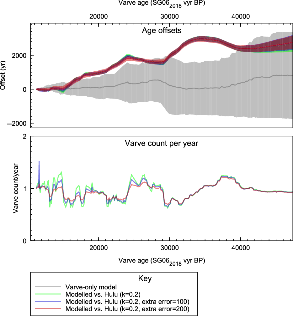
Figure 2 This shows the differences between the Lake Suigestu varve age model (Schlolaut et al. Reference Schlolaut, Staff, Brauer, Lamb, Marshall, Bronk Ramsey and Nakagawa2018) and preliminary age models based on both the varves and the Hulu timescale (Cheng et al. Reference Cheng, Lawrence Edwards, Southon, Matsumoto, Feinberg, Sinha, Zhou, Li, Li and Xu2018), as plotted against the varve chronology age (before AD 1950). The three models presented here are all based on the same P_Sequence rigidity (k=0.2) but with different levels of additional error accounted for (0, 100, and 200 years). The higher the extra uncertainty, the closer the model follows the varve chronology, particularly in the younger section of the record. The older section is little affected by this degree of additional uncertainty.
In all models the radiocarbon offset between the Suigetsu data and the reservoir-corrected Hulu data was treated as an unknown, with a prior of U(–100,100). The models all showed a consistently negligible offset between the datasets: 21±19 for k=0.1, 12±17 for k=0.2, 5±16 for k=0.3, 8±19 for k=0.2 with an extra error of 100, and –1±32 for k=0.2 with an extra error of 200. In all cases but the last, the SG06 dates were slightly older when compared to the corrected Hulu data suggesting, if anything, the Hulu reservoir (or dead carbon fraction) to be marginally over estimated. However, all are, within error limits, consistent with a zero systematic offset.
The methodology provides two pieces of information for inputting into the calibration curve. Firstly, a marginal posterior estimate for the U-Th age associated with each radiocarbon date within the core: this information has been summarized in the supplementary information of this paper using the mean and standard deviation (as used for the incorporation into IntCal) and the highest posterior density (hpd) ranges at 68.2 and 95.4% probabilities. Secondly, a correlation coefficient matrix for all distinct levels has been generated; given the nature of the underlying varve chronology there is a considerable degree of correlation between closely spaced dates (implying that calendar age shifts to one require others nearby to be similarly shifted). It should be noted that there is also some correlation across the dataset as a whole because of the shared uncertainty in the reservoir age of the Hulu Cave speleothems.
INTEGRATION WITH INTCAL20
The revised Suigetsu dataset is included within the IntCal20 calibration curve, as described by Heaton et al. (Reference Heaton, Blaauw, Blackwell, Bronk Ramsey, Reimer and Scott2020 in this issue). The marginal posteriors for the model described in the previous section (including the correlation matrix), are treated as priors in the construction of the IntCal curve. The main distinguishing features of this dataset are: i) that there is no dead carbon or reservoir effect required, and ii) the correlated nature of the calendar age uncertainty. The latter is fully incorporated into the main curve construction through suitable adaptation of the errors-in-variables (see Heaton et al. Reference Heaton, Blaauw, Blackwell, Bronk Ramsey, Reimer and Scott2020 in this issue). Correctly modelling and including this calendar age covariance, also present within the Cariaco, Pakistan, and Iberian margin chronologies, into curve construction is important. It improves our ability to distinguish what is noise and what is signal by making it easier to identify common features when combining the full set of varied records; and means that more of the structure and shape of the Suigetsu record is maintained within the final IntCal20 compilation.
A useful aspect of the methodology used for IntCal20 is that we are able to retrieve marginal posterior dates for each of our dated levels within the Suigetsu (SG06) core. These estimates make use of all of the other data included within the calibration curve, and so provide our best estimate of the age of the sediments within SG06. A comparison of this final age model to our preliminary model, and to the varve-only model, will be discussed in the next section.
DISCUSSION
The first point for discussion is the degree to which the preliminary and final age models differ from the varve-based chronology. In the younger part of the sequence (down to about 28 kvyr BP in the varve chronology) the offsets were expected and are similar to those seen for IntCal13 (Reimer et al. Reference Reimer, Bard, Bayliss, Beck, Blackwell, Bronk Ramsey, Buck, Cheng, Edwards and Friedrich2013). However, for the period between 30 and 40 kvyr BP the offsets are much better constrained by the new Hulu data. This shifts the SG06 data significantly older in this period with sections of both apparent under-counting and over-counting seen in the varve chronology. Were the evidence for this only from the Hulu dataset, we might have worried that the U-Th chronology of these speleothems had a problem in this period. However, it is clear that much of the available marine data, including the U-Th dated corals, share the pattern seen here, even though there is some scatter due to diagenesis. This is evident in the placement of the IntCal09 (Reimer et al. Reference Reimer, Baillie, Bard, Bayliss, Beck, Blackwell, Bronk Ramsey, Buck, Burr and Edwards2009) curve relative to IntCal13. Here we can see then the real strength in being able to draw on these very different independent datasets.
While much of the relative varve chronology is supported by the final age-scale, the places where there are deviations are worth considering. As a first step we determined which of the deviations are outside the uncertainty range of the interpolated sedimentation rates using a resolution of 5 and 50 cm. This revealed that in only two significant core intervals could the U-Th adjusted chronology not be supported by the varve data: between ~1730 and ~1820 cm composite depth (~15 to 18 kvyr BP) and between ~2700 and ~2880 cm (~29.3 to 32.6 kvyr BP). In either case the sedimentation rates of the final age-scale are lower than the smallest sedimentation rates within the uncertainty range of the varve model, so that an age difference remains: in the upper interval ~300 years and in the lower interval ~700 years. If these offsets are indeed due to an error in the varve model, then there are only a limited number of potential reasons for that. Since the varve model is interpolated, a systematic under-representation of, in this case, small varve thicknesses could be a reason. This means that if environmental conditions which lead to low sediment accumulation were also unfavourable for varve formation, then thin varves are underrepresented. This in turn would lead to a problem in the interpolation (Schlolaut et al. Reference Schlolaut, Staff, Brauer, Lamb, Marshall, Bronk Ramsey and Nakagawa2018) resulting in too high an interpolated sedimentation rate. In particular the lower of the two intervals is suspicious in this regard, since it almost coincides with microfacies zone II.a2 (Schlolaut et al. Reference Schlolaut, Staff, Brauer, Lamb, Marshall, Bronk Ramsey and Nakagawa2018). This interval is characterized by a low frequency of seasonal layers, with a very high proportion of the occurring layers being of low quality, i.e. poorly distinguishable. Since a microfacies zone indicates specific environmental conditions different from those of other microfacies zones, this offset in the age model might indeed be due to the effect of these environmental conditions on varve formation. However, without independent proof this explanation remains theoretical.
Next, we consider how close the prior estimates from our preliminary timescale compare to the output from the overall IntCal model. The relative offsets are shown in Figure 3. Here it can be seen that within the 2-σ uncertainty envelopes plotted, the two are in reasonable agreement. In general the final age model is pulled slightly further away from the varve-only model and is quite close to the preliminary model (against Hulu) that we would have obtained with a lower model rigidity (see Figure 1 above). This is to be expected, because, within IntCal, the Hulu data are still influencing the calendar age of SG06; this is not an argument for using a less rigid preliminary model, since that would effectively just down-weight the importance of the relative ages from the varve chronology.

Figure 3 The differences between the varve age model (Schlolaut et al. Reference Schlolaut, Staff, Brauer, Lamb, Marshall, Bronk Ramsey and Nakagawa2018), the preliminary age model (in green) based on both the varves and the Hulu timescale (Cheng et al. Reference Cheng, Lawrence Edwards, Southon, Matsumoto, Feinberg, Sinha, Zhou, Li, Li and Xu2018) and the final age model based on all data within IntCal20 (in magenta), as plotted against the varve chronology age (before AD 1950).
Finally, we consider what can be learnt from the differences between this dataset and that from the Hulu speleothem. To do this we have also constructed a Bayesian spline-based curve, again implementing the same errors-in-variables method used in the main IntCal20 construction, but using only the Suigetsu data; and another just for the Hulu speleothem data, but this time without the allowance for the dead carbon fraction to vary independently by up to ±50 years used for the preliminary timescale (this is to retain as much of the authentic higher frequency signal as possible within that dataset for comparison with Suigetsu). The comparison between these two spline curves is shown in Figure 4.

Figure 4 A comparison of spline compilations of the two datasets discussed here, Suigetsu (green) and Hulu (red, not incorporating extra uncertainty for the reservoir offset). The Suigetsu data is on the preliminary timescale. The comparison shows that there is much more high-frequency signal in the Suigetsu record. The errors here are 1 σ.
What is clear from this is that the Suigetsu data appear to have much more high-frequency signal than the Hulu data. This could be noise, or it could be a real signal. At the Laschamp excursion (circa 41k cal BP) the uncertainties become large in the Suigetsu data, and so it is more useful to focus on the period where the measurement uncertainty is smaller (20–35k cal BP; see Figure 5).

Figure 5 A comparison of spline compilations of the two datasets discussed here, Suigetsu (green) and Hulu (red, not incorporating extra uncertainty for the reservoir offset) over the period from 20–35k calBP.
If we were to smooth the Suigetsu dataset sufficiently, it would be possible to make it look more like that of the speleothem. However, this does not really tell us much about the causes for the difference. More instructive is to run a deconvolution of the Hulu data to see what extra signal might be present there. We have tried this using MatLab and a linear ramp filter with a mean weight of 420 years. The results of this exercise are shown in Figure 6 where you can see that this does actually accentuate some features seen in the Suigetsu data, suggesting that the signals seen in Suigetsu are at least not entirely noise. The implication of this is that the offset from the atmosphere seen in Hulu may be more of a reservoir effect than a dead carbon fraction. Of course the real test of this will be as more high-resolution tree-ring data become available. In the meantime, the high-resolution data from the Cariaco Basin provides data-points within the IntCal curve to test the signals seen in the two datasets. The final IntCal20 curve does contain much of the high-frequency components seen within the Suigetsu dataset, but somewhat muted; correctly we would argue, because there will undoubtedly be some noise as well as signal, and only testing against other datasets can distinguish between these.

Figure 6 A comparison of spline compilations of the two datasets discussed here, Suigetsu (green) and Hulu (magenta) over the period from 20–30k calBP with the Hulu dataset transformed using a deconvolution algorithm (linear ramp with mean of 420 years, using the MatLab deconv function).
CONCLUSIONS
The Suigetsu dataset has provided us with important information for this iteration of the calibration curve. In particular, it provides a direct atmospheric and unfiltered dataset, which is closest in nature to the types of terrestrial samples many users of radiocarbon will be using for chronological purposes. We would argue that the data from this series suggest that the speleothem record from Hulu (Cheng et al. Reference Cheng, Lawrence Edwards, Southon, Matsumoto, Feinberg, Sinha, Zhou, Li, Li and Xu2018) may not contain all of the high-frequency components of the atmospheric variation in radiocarbon. On the other hand, the Suigetsu record on its own would not be useful without the age constraints provided by the speleothem and coral data with their direct U-Th ages, so the high-frequency signals in the Suigetsu dataset can really only be tested against the high-resolution marine data from Cariaco (Hughen et al. Reference Hughen, Lehman, Southon, Overpeck, Marchal, Herring and Turnbull2004), and, where available, limited floating tree-ring sequences (for example, Turney et al. Reference Turney, Palmer, Bronk Ramsey, Adolphi, Muscheler, Hughen, Staff, Jones, Thomas, Fogwill and Hogg2016). All of these different datasets together provide us with a network of information that makes the calibration curve more robust.
ACKNOWLEDGMENTS
We would like to acknowledge the support of the UK Natural Environment Research Council for helping to support this research both through grants (NE/F004400/1, NE/H007865/1) and for support of the NERC radiocarbon facility at Oxford and East Kilbride (SUERC). Valuable support for the varve chronology was also provided by the Japan Society for the Promotion of Science (JSPS KAKENHI grant JP15H06905). We would also like to thank Paula Reimer for her support for this research and leadership of the IntCal group.
SUPPLEMENTARY MATERIAL
To view supplementary material for this article, please visit https://doi.org/10.1017/RDC.2020.18


