


1. Introduction
Nature provides a host of examples of interacting bodies through a fluid with surprising behaviours. These range from a single, passive body like an auto-rotating maple seed (Lentink et al. Reference Lentink, Dickson, van Leeuwen and Dickinson2009) to a large number of synchronized, active bodies which interact with the surrounding fluid, like fish schooling or bird flocks (Weihs Reference Weihs1973; Mora et al. Reference Mora, Walczak, Del Castello, Ginelli, Melillo, Parisi, Viale, Cavagna and Giardina2016). The latter is particularly interesting since, due to the presence of more than one body, each individual has to interact with an ambient fluid which is disturbed by the surrounding individuals. These interactions can be exploited by the individual to extract energy from the fluid and move in a more efficient manner than if it were in isolation. Although the main reason why animals form schools or flocks may not be entirely clear yet, it is well known that animals benefit from collective motion in terms of flow interaction (Weimerskirch et al. Reference Weimerskirch, Martin, Clerquin, Alexandre and Jiraskova2001; Becker et al. Reference Becker, Masoud, Newbolt, Shelley and Ristroph2015).
This beneficial interaction is not restricted to a large number of bodies, but it is also observed at its minimal expression for two-body configurations. For example, Liao et al. (Reference Liao, Beal, Lauder and Triantafyllou2003) observed that a trout behind the wake of a cylinder adapted its body kinematics to extract energy from the vortices of the cylinder's wake. They attributed this phenomenon to a beneficial interaction with the oncoming vortices, which they denoted as Kármán gait. Even more stunning are the results from Beal et al. (Reference Beal, Hover, Triantafyllou, Liao and Lauder2006), who observed that a dead fish can overcome its own drag in the wake of a cylinder provided its resonant frequency matches that of the von Kármán vortex sheet. It can be argued that the beneficial flow interaction in the previous examples is merely due to the lower average streamwise velocity of the von Kármán vortex sheet wake. However, several studies have shown that swimmers are less efficient when isolated (i.e. in a clean free stream) than when swimming in reverse von Kármán streets, like those produced by thrust-producing, oscillating foils in a free stream (Platzer et al. Reference Platzer, Jones, Young and Lai2008) or self-propelling oscillating bodies (Alben & Shelley Reference Alben and Shelley2005). In particular, Boschitsch, Dewey & Smits (Reference Boschitsch, Dewey and Smits2014), Muscutt, Weymouth & Ganapathisubramani (Reference Muscutt, Weymouth and Ganapathisubramani2017) and Kurt & Moored (Reference Kurt and Moored2018) found that, for an inline tandem configuration of two oscillating foils, the distance and phase shift between the motion of the foils can always be adjusted such that the follower foil interacts with the oncoming vortices extracting energy from the flow, thus confirming the Kármán gait hypothesis proposed in Liao et al. (Reference Liao, Beal, Lauder and Triantafyllou2003) and Streitlien, Triantafyllou & Triantafyllou (Reference Streitlien, Triantafyllou and Triantafyllou1996).
However, in the aforementioned examples the bodies were immersed in a free stream with their horizontal position held fixed. Consequently, the configuration of the collective motion is not determined by the fluid interaction. Conversely, when the bodies self-propel, the configuration cannot be imposed but is the one that results from the equilibrium of the hydrodynamic forces due to flow-mediated interactions. Ramananarivo et al. (Reference Ramananarivo, Fang, Oza, Zhang and Ristroph2016) and Newbolt, Zhang & Ristroph (Reference Newbolt, Zhang and Ristroph2019) experimentally studied the case of two airfoils in an inline tandem configuration which self-propelled due to an imposed heaving motion with a varying phase shift. They found that, for a given phase shift, stable configurations emerged at quantized equilibrium distances; and that this distance was linearly proportional to the phase shift. However, no measurements of the efficiency were provided, leaving open-ended the question of whether tandem configurations of self-propelled bodies can benefit from flow interactions. In this regard, numerical simulations have proven to be very useful, since they can provide quantitative data of the flow field, but also of the forces and moments acting on the bodies. Lin et al. (Reference Lin, Wu, Zhang and Yang2019) numerically simulated two self-propelling two-dimensional (2-D) foils undergoing a heaving and pitching motion, finding that the follower always benefits from the flow interaction, whereas the lead foil can benefit only if both foils are close. Similar studies are found in the literature where the bodies are modelled as flexible foils and self-propulsion is achieved by way of a passive flexion of the body (Zhu, He & Zhang Reference Zhu, He and Zhang2014; Peng, Huang & Lu Reference Peng, Huang and Lu2018a; Ryu et al. Reference Ryu, Yang, Park and Sung2020), or where the deflection of the body is fully prescribed (Maertens, Gao & Triantafyllou Reference Maertens, Gao and Triantafyllou2017). In all these cases, similar qualitative conclusions are extracted from these works, suggesting that the same main flow mechanism interaction is present in all these examples of self-propelled collective locomotion.
Additional studies have focused on the effect of the size of the bodies (Peng, Huang & Lu Reference Peng, Huang and Lu2018b); the kinematics of the prescribed degrees of freedom (namely plunging or pitching motion) (Heydari & Kanso Reference Heydari and Kanso2020; Lin et al. Reference Lin, Wu, Zhang and Yang2021); or the stable schooling configurations with multiple individuals (Dai et al. Reference Dai, He, Zhang and Zhang2018; Park & Sung Reference Park and Sung2018; Peng, Huang & Lu Reference Peng, Huang and Lu2018c; Lin et al. Reference Lin, Wu, Zhang and Yang2020). However, very few works are found in the literature which consider a three-dimensional (3-D) flow, all the previous examples being restricted to 2-D configurations. Some examples of 3-D analyses include Daghooghi & Borazjani (Reference Daghooghi and Borazjani2015), who numerically investigated the performance of an ‘infinite’ school of mackerel with a rectangular pattern; and Li et al. (Reference Li, Kolomenskiy, Liu, Thiria and Godoy-Diana2019), who analysed the energetic benefit of a two-fish-school configuration where the kinematics of both fish was that of self-propulsion, but their relative distance was fixed. However – to our knowledge – the only 3-D study where the bodies self-propel and their dynamics are determined from the fluid–structure interaction is that of Verma, Novati & Koumoutsakos (Reference Verma, Novati and Koumoutsakos2018). They performed numerical simulations of a pair of 3-D zebrafish-like swimmers, where the undulation of the body of one of the swimmers (follower) is controlled to keep a relative position with respect to the other swimmer (leader). The controller is based on a deep reinforcement algorithm developed for a 2-D model of the same pair of zebrafish-like swimmers. In that study, the relative position between the leader and the follower is defined a priori with the objective of testing the developed control law. The chosen a priori location is expected to produce a beneficial fluid interaction between the swimmers. However, a systematic analysis of the performance of the swimmers at different relative positions is not performed.
This lack of 3-D studies may be explained by the computational cost. However, it is known that the wake pattern of a self-propelled body significantly differs from two to three dimensions (Gazzola et al. Reference Gazzola, Chatelain, van Rees and Koumoutsakos2011): from a reverse von Kármán vortex street in two dimensions to a diverging wake of vortex rings (VRs) in three dimensions. This could lead to significant differences of 3-D stable positions of the collective and of their associated performance when compared to 2-D counterparts. First of all, the stable quantized positions observed by Ramananarivo et al. (Reference Ramananarivo, Fang, Oza, Zhang and Ristroph2016) and Newbolt et al. (Reference Newbolt, Zhang and Ristroph2019) on a von Kármán vortex street may no longer emerge on a 3-D bifurcating wake. Secondly, on a 2-D vortex street the only dissipation mechanism is viscosity; however, 3-D mechanisms can lead to vortex breakdown at much shorter distances. Hence, different vortical interactions might be expected in three dimensions with respect to two, which could alter the performance of the bodies. In summary, it is not clear if the main conclusions of tandem self-propelled bodies obtained from 2-D studies are applicable to 3-D scenarios.
In the present study, we analyse the problem of two self-propelled finite-aspect-ratio plates in tandem configuration. Particularly, the plates have chordwise flexibility (similar to the studies of Quinn, Lauder & Smits (Reference Quinn, Lauder and Smits2014, Reference Quinn, Lauder and Smits2015), Yeh & Alexeev (Reference Yeh and Alexeev2014) and Hoover et al. (Reference Hoover, Cortez, Tytell and Fauci2018)) and self-propel due to an imposed heaving motion of their leading edge. The main focus of the study is to identify which are the equilibrium positions in this 3-D scenario, and to characterize the performance of the system at these equilibrium positions. Additionally, the main similarities to/differences from the 2-D configurations found in the literature are also highlighted.
The paper is structured as follows: § 2 describes the problem and the numerical methodology; in § 3 the main results are discussed; and finally the main conclusions of the study are gathered in § 4.
2. Methodology
2.1. Problem description
Two self-propelling plates in tandem configuration immersed in an otherwise undisturbed fluid are considered. The plates have a rectangular planform of chord  $C$ and span $b$; thickness $e$; uniform density $\rho _s$; and they are flexible along the chordwise direction. Under the tandem arrangements considered, one of the flappers swims downstream of the other. We denote the flapper swimming downstream as follower and the upstream flapper as leader. Hence, variables related to the follower and leader are indicated hereafter with the subscripts $f$ and $l$, respectively.
The vertical motion of the leading edge of the flappers is prescribed as sinusoidal functions, namely
 \begin{equation} Z_l(t) = A_l\cos{(2{\rm \pi} ft)}, \quad Z_f(t) = H + A_f\cos{(2{\rm \pi} f t - \phi)}, \end{equation}
where  $A_i$ is the heaving amplitude of the $i$ flapper, $f$ is the frequency of oscillation, $\phi$ is the phase offset and $H$ is the mean vertical offset between the flappers. These magnitudes are sketched in figure 1, alongside the instantaneous horizontal distance, $D(t) = X_f(t) - X_l(t)$, where $X_i$ is the horizontal position of the leading edge of the $i$ flapper.

Figure 1. Side view of the schooling configuration. Each flapper has a prescribed heaving motion about a fixed vertical pivoting position (represented as a red dot). The vertical offset between the follower's and leader's pivoting position is denoted as  $H$. Distance $D(t)$ is the instantaneous horizontal distance between the flappers’ leading edges.
The flappers share the same fixed plane of symmetry along the spanwise ( $y$) direction (i.e. they are aligned), and their leading edge is always parallel to the $y$ axis. Hence, while the vertical motion of the leading edge of the flappers is prescribed, their horizontal motion results from the fluid–structure interaction. Note that in this configuration, the only external forces acting on the plates are the hydrodynamic forces and the driving force that imposes the vertical motion of the leading edge of the flappers. In particular, no gravitational force is considered in this study.
The fluid surrounding the flappers is governed by the Navier–Stokes equations of incompressible flow for a Newtonian fluid, namely
 $$\begin{gather} \boldsymbol{\nabla}\boldsymbol{\cdot}\boldsymbol{u} = 0, \end{gather}$$
 $$\begin{gather}\frac{\partial \boldsymbol{u}}{\partial t} + (\boldsymbol{u}\boldsymbol{\cdot}\boldsymbol{\nabla})\boldsymbol{u} ={-}\frac{1}{\rho}\boldsymbol{\nabla} p + \nu\nabla^2\boldsymbol{u}, \end{gather}$$
where  $\boldsymbol {u}$ is the flow velocity, $p$ is the fluid pressure, $\rho$ is the fluid density and $\nu$ is the fluid kinematic viscosity.
One of the objectives of the present study is to find stable equilibrium positions of the flappers in the  $H\text {--}\phi$ plane. The rest of the parameters that define the problem are kept fixed: the aspect ratio of the flappers, $b/C$, and their non-dimensional thickness, $e/C$; the heaving amplitude is set equal for both flappers, $A_l \equiv A_f = A$; the Reynolds number, $Re = VC/\nu$, where $V = 2{\rm \pi} A f$ is the maximum vertical velocity of the leading edge of the flappers; the density ratio, $\varrho = \rho _s/\rho$; and the non-dimensional natural frequency, $\omega ^* = \omega _n/(2{\rm \pi} f)$, where $\omega _n$ is the first natural frequency of the flapper's elastic response in vacuum. The values of these parameters are presented in table 1.
Table 1. Parameters of the problem under study.

To select the elastic properties of the flapper (i.e. its natural frequency), two different simulations of self-propelled isolated flappers with finite aspect ratio (i.e. 3-D simulations) were performed with  $\omega ^* = 2.17$ and $4.59$, choosing for the present study the case yielding maximum propulsive speed. The range for values of $\omega ^*$ used in the prospective 3-D simulations was selected after performing a finer parametric study of the equivalent 2-D problem, similar to that presented in Arora et al. (Reference Arora, Kang, Shyy and Gupta2018).
2.2. Computational set-up
To simulate the chordwise flexibility of a flapper the lumped-torsional flexibility model of Arora et al. (Reference Arora, Kang, Shyy and Gupta2018) is used. Under this approach, a flapper is discretized into  $N_B$ rigid bodies linked to each other by means of torsional springs. The stiffness of these torsional springs is computed to match $\omega ^*$. A sketch of the multi-body model of a flapper is provided in figure 2. For a given flapper, its rigid bodies are labelled as $j = 1,\ldots,N_B$. Each body is a rectangular prism of span $b$, length $c$ and thickness $e$, separated a distance $d = e/2$ from the torsional spring that connects it to the consecutive body. Consequently, the relative attitude of body $j$ with respect to its predecessor $j-1$ is given by the angle $\theta _j$ (see figure 2b).

Figure 2. (a) A 3-D representation of the multi-body model of a flapper. (b) Side view ( $x\text {--}z$ plane) of the multi-body model. Blue spirals are the torsional springs and $\theta _j$ is the relative deflection angle of body $j$ with respect to body $j-1$, similar to Arora et al. (Reference Arora, Kang, Shyy and Gupta2018).
Under the previous model, each flapper has  $2 + N_B$ degrees of freedom, namely horizontal ( $X$) and vertical ( $Z$) translation of the leading edge and $N_B$ relative rotations of the bodies. Therefore, it is possible to express the equations that govern the dynamics of the flappers in the general form (Featherstone Reference Featherstone2014)
 \begin{equation} {\boldsymbol{\mathsf{H}}}(\boldsymbol{q})\ddot{\boldsymbol{q}} = \boldsymbol{\xi} - {\boldsymbol{\mathsf{c}}}(\boldsymbol{q},\dot{\boldsymbol{q}}) + \boldsymbol{\xi}_{h}, \end{equation}
where  $\boldsymbol {q}$ is the vector of generalized coordinates (i.e. the degrees of freedom of the system), ${\boldsymbol{\mathsf{H}}}$ is the generalized inertia matrix, ${\boldsymbol{\mathsf{c}}}$ is the generalized bias force vector, $\boldsymbol {\xi }$ is the vector of the generalized forces (accounting for the torsional springs) and $\boldsymbol {\xi }_h$ is the vector of the generalized hydrodynamic forces. Although in (2.3) only the dependence on $\boldsymbol {q}$ and $(\boldsymbol {q},\dot {\boldsymbol {q}})$ is made explicit for ${\boldsymbol{\mathsf{H}}}$ and ${\boldsymbol{\mathsf{c}}}$, respectively, they both implicitly depend on the geometric and inertia properties of the flappers.
The vector of generalized coordinates is defined as  $\boldsymbol {q} = [\boldsymbol {q}_u, \boldsymbol {q}_p]^\top$, where $\boldsymbol {q}_u = [X_l, \theta _{l,1},\ldots, \theta _{l,N_B}, X_f, \theta _{f,1},\ldots, \theta _{f,N_B}]^\top$ is the vector of unknown generalized positions, and $\boldsymbol {q}_p = [Z_l, Z_f]^\top$ is the vector which contains the prescribed generalized positions, given by (2.1a,b). Likewise, $\boldsymbol {\xi } = [\boldsymbol {\xi }_u, \boldsymbol {\xi }_p]$, where $\boldsymbol {\xi }_u = -K[0, \theta _{l,1},\ldots, \theta _{l,N_B}, 0, \theta _{f,1},\ldots, \theta _{f,N_B}]^\top$, and $\boldsymbol {\xi }_p = [F_{p,l}, F_{p,f}]^\top$ contains the unknown reaction vertical forces acting on the leading edge. In the present implementation, a reduced system of (2.3) is solved to compute $\boldsymbol {q}_u$, $\dot {\boldsymbol {q}}_u$ and $\ddot {\boldsymbol {q}}_u$, as detailed in Arranz (Reference Arranz2021). After that, one can solve for the reactive forces acting on the leading edge. For the present study, $N_B = 5$, based on the work of Arora et al. (Reference Arora, Kang, Shyy and Gupta2018).
Equations (2.2) and (2.3) are solved together using an in-house code, TUCANMB (Arranz Reference Arranz2021). In particular, the flow is solved by means of direct numerical simulations, where the presence of the body in the fluid is modelled using the immersed boundary method proposed by Uhlmann (Reference Uhlmann2005). On the other hand,  ${\boldsymbol{\mathsf{H}}}$ and ${\boldsymbol{\mathsf{c}}}$ of (2.3) are computed using the robotic algorithm presented in Felis (Reference Felis2017). The coupling between the fluid and the dynamic equations along time is done in a staggered way, usually referred to as weak coupling. Interested readers can find more details of the algorithm in Arranz (Reference Arranz2021).
The computational fluid domain is a rectangular prism of size  $16C\times 6C\times 8C$ along the streamwise, spanwise and vertical directions, respectively. Note that the same computational fluid domain was used in Yeh & Alexeev (Reference Yeh and Alexeev2014) for similar simulations of an isolated 3-D self-propelled flexible plate. The flappers are located inside a refined region with uniform grid size, $\Delta r$, extended from $[-0.5C,\ 0.5C]$ along the $y$ axis, $[-C,\ C+H]$ along the $z$ axis and $[-6.5C,\ L_{x}]$ (where $L_x$ ranged from $-2C$ to $4C$, depending on $\bar {D}$) along the $x$ axis. Note that those distances are given with respect to the cuboid centroid. Moreover, for cases with $H = 0.6C$ the total domain is also enlarged $0.6C$ in the positive $z$ direction. Outside this uniformly refined region, the mesh has a constant stretching of $0.8\,\%$ in all directions.
The grid size,  $\Delta r$, is determined after performing a grid sensitivity analysis, leading to the conclusion that $\Delta r = C/50$ accurately captures the dynamics of the problem, whereas with $\Delta r = C/80$ the flow details and temporal evolution of the forces are accurately represented. Consequently, the simulations are performed with $\Delta r = C/50$. Only for those configurations in which flow visualizations and temporal histories of force and power are presented, the simulations are performed with $\Delta r = C/80$. Likewise, the time step is selected to be $\Delta t/T = 5\times 10^{-4}$ and $4\times 10^{-4}$, where $T = 1/f$ is the flapping period, for $\Delta r = C/50$ and $C/80$, respectively, ensuring ${CFL} = U_{max}\Delta t/\Delta r < 0.2$ (where $U_{max}$ is the maximum flow velocity in the domain). Interested readers can find more details of the grid sensitivity analysis in the Appendix.
A constant horizontal velocity,  $U_\infty$, is imposed at the inflow boundary; an advective boundary condition is imposed at the outflow boundary; and free-slip boundary conditions are imposed at the lateral boundaries. With the present set-up, the flappers could reach the inflow or outflow boundaries if their mean advance velocity (denoted as propulsive speed, $\bar {U}_p$, in the following sections) is higher or lower than $U_\infty$, respectively. Therefore, the inflow velocity must be set equal to $U_\infty \equiv \bar {U}_p$ so that the flappers remain in the refined region of the computational domain. Since $\bar {U}_p$ is unknown a priori, simulations are started with an initial guess of $U_\infty$, denoted as $U_i^0$, which is updated every $k$th time step, by means of the relaxation equation:
 \begin{equation} U_i^k = (1 - \beta)U_i^{k-1} + \beta \dot{X}_{l}^{k-1}, \end{equation}
where  $\beta$ is a small parameter set to $\Delta t/T$ and superscripts indicate the time step where the variable is evaluated. After a transient, the horizontal position of the flappers oscillates around a fixed value, as well as $U_i$. It turns out that the average value of $U_i$ over a complete oscillation is a good estimate of the mean propulsive velocity. Therefore, $U_\infty$ is set to this average value, and the simulation is continued with this constant inflow velocity. Only the results of this last phase of the simulations are reported in this paper, after discarding the initial transient.
Finally, it should be pointed out that our simulations do not include any mechanism to prevent the two flexible plates from touching. Indeed, this occurs for some simulations with  $\phi <0$ and $D_0/C = 1.5$, which have been discarded. The two flappers of all simulations presented in this work have been checked to not overlap at any time.
2.3. Performance indicators
After an initial transient, the flappers self-arrange into a stable configuration, with a constant mean separation distance,  $\bar {D}$, and mean propulsive speed, $\bar {U}_p$, over a cycle. These magnitudes are computed as
 \begin{equation} \bar{D} = \frac{1}{T}\int^{T_*}_{T_*-T} D(t) \,\textrm{d} t,\quad \bar{U}_p = U_\infty - \frac{1}{T}\int^{T_*}_{T_*-T} \dot{X}_l \,\textrm{d} t, \end{equation}
where  $T_*$ is the last computed full cycle of the simulation.
The performance of a self-propelled flapper is computed in terms of its average power consumption over a flapping cycle, namely
 \begin{equation} \bar{P}_i = \frac{1}{T}\int^{T_*}_{T_*-T} \max{(P_{i},0)}\, \textrm{d} t, \end{equation}
where  $P_{i} = F_{p,i}\cdot \dot {Z}_i$, $F_{p,i}$ being the vertical component of the reaction force acting on the leading edge of the $i$ flapper. Neglecting the negative power contribution in (2.6) entails that the elastic storage of power is not considered. This approach is similar to the one adopted in Berman & Wang (Reference Berman and Wang2007) and Vejdani et al. (Reference Vejdani, Boerma, Swartz and Breuer2018). In the following discussion the performance of a given flapper in tandem configuration is assessed in terms of a comparison with the same flapper in isolation. To that purpose the power ratio of the $i$ flapper is defined as $\varPi _i = \bar {P}_i/\bar {P}_s$, where $\bar {P}_{s}$ is the averaged power of the isolated flapper.
As an additional measure of performance, the propulsive efficiency  $\eta$ is defined as the ratio between the total useful kinetic energy and the total power consumption:
 \begin{equation} \eta = \frac{m \bar{U}_p^2}{T(\bar{P}_l + \bar{P}_f)}, \end{equation}
where  $m$ is the mass of each flapper. The equivalent propulsive efficiency that the tandem system would have if no interaction between flappers occurred is also defined:
 \begin{equation} \eta_s = \frac{m \bar{U}_{p,s}^2}{2T\bar{P}_s}. \end{equation}
3. Results
3.1. Emergent patterns and overall dynamics
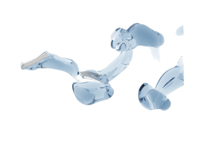
For reference, the case of the isolated flapper is presented first. The flapper self-propels at a mean speed,  $\bar {U}_{p,s} = 0.88V$, shedding a VR during each stroke. The VRs move away from the flapper with an oblique trajectory due to their own induced velocity, leading to a bifurcating wake (Kurt, Eslam & Moored Reference Kurt, Eslam and Moored2020). These vortices are visible in figure 3(a), which shows a visualization of the flow around the isolated flapper at mid-downstroke. The deflection of the flapper during a cycle is depicted in figure 3(b). Note that the upstroke and the downstroke deflection patterns are symmetric. At the beginning of a stroke, the flapper is almost horizontal, whereas the largest deflection occurs at mid-stroke. Consequently, there is a phase offset of $\sim {\rm \pi}/2$ between the heaving motion and the deflection. Such a phase offset is characteristic of oscillating foils with low mass ratios ( $\equiv \rho _s e/ \rho C = 0.2$, in the present study) and is linked to an increase of the fluid forces during the mid-stroke, which dominate over inertia for low mass ratios (Dai, Luo & Doyle Reference Dai, Luo and Doyle2012; Arora et al. Reference Arora, Kang, Shyy and Gupta2018). Yeh & Alexeev (Reference Yeh and Alexeev2014) found a similar phase offset for a flexible self-propelling plate of finite span when its plunging frequency was adjusted to yield maximum propulsive speed.

Figure 3. (a) Flow visualization around the isolated, self-propelled, flapper at mid-downstroke. Flow is visualized in terms of iso-surfaces of the  $Q$-criterion for $Q/f^2 = 0.1$. (b) Bending pattern of the flapper's chordline during the downstroke (solid) and upstroke (dashed). Dotted line corresponds to the trajectory of the leading edge. (c,d) Flow visualization around the flappers in tandem formation. Flow is visualized in terms of iso-surfaces of the $Q$-criterion for $Q/f^2 = 0.5$: (c) $H = 0.6C$, $\phi = 180^\circ$ and (d) $H = 0$, $\phi = 0^\circ$.
Figure 4 depicts the streamwise,  $\langle u \rangle$, and vertical, $\langle w \rangle$, velocities of the fluid averaged over a cycle and along the flapper's span $y/C = [-0.25, 0.25]$. Note that, for the averaging, a Galilean reference frame moving at a constant horizontal speed, $\bar {U}_{p,s}$, was used. The averaged wake left by the VRs results in a bifurcating momentum jet. Note that this wake pattern is not restricted to flexible, 3-D self-propelling flappers, but is general to oscillating bodies, like rigid wings, immersed in a free stream within the typical range of Strouhal for propulsion, namely $0.15 \leq {\boldsymbol {St}} \leq 0.5$ (Taylor, Nudds & Thomas Reference Taylor, Nudds and Thomas2003). In particular, the diverging wake pattern made of shed VR is the common trace of low-aspect-ratio oscillating wings (Dong, Mittal & Najjar Reference Dong, Mittal and Najjar2006; Buchholz & Smits Reference Buchholz and Smits2008). This wake pattern clearly differs from the reverse von Kármán wake observed in 2-D self-propelled plates (Alben & Shelley Reference Alben and Shelley2005; Hua, Zhu & Lu Reference Hua, Zhu and Lu2013).

Figure 4. Velocity field of the isolated self-propelled flapper, averaged over one cycle and over  $y/C = [-0.25, 0.25]$. (a) Horizontal component of the velocity, $(\langle u \rangle - \bar {U}_{p,s}) / \bar {U}_{p,s}$, and (b) vertical component of the velocity, $\langle w \rangle / \bar {U}_{p,s}$. The black line corresponds to the mean position of the flapper.
We now turn our attention to the emergent dynamics found in the tandem simulations. A total of 24 tandem configurations were simulated. They are characterized by the follower's vertical offset,  $H$, the phase shift, $\phi$, and the ensuing equilibrium distance, $\bar {D}$. Under the initial separation distances considered (i.e. $D_0/C = [1.5$– $3]$), a single $\bar {D}$ was found for each $\phi$. The only exception is case $\phi = 0^\circ$, for which two equilibrium distances coexisted ( $\bar {D}/C \approx 1$ and $\bar {D}/C \approx 3.4$), depending on $D_0$. In order to differentiate them, we assign $\phi = 0^\circ$ to those configurations for which $\bar {D}/C \approx 1$ (obtained with $D_0/C = 1.5$), whereas $\phi = 360^\circ$ is used for the tandem configurations where $\bar {D}/C \approx 3.4$ (obtained with ${D_0/C = 3}$).
For illustration, figure 3 displays flow visualizations of two of the cases. Figure 3(c) displays the flow corresponding to the case  $H = 0.6C$ and $\phi = 180^\circ$, leading to $\bar {D}/C = 2.2$ (i.e. the horizontal gap between the trailing edge of the leader and the leading edge of the follower is approximately equal to $1.2C$). It can be appreciated that the flow surrounding the leader is virtually unaffected by the follower, whereas the follower is swimming across the leader's wake vortices. Downstream of the follower, the wakes of the flappers interact yielding a different wake structure from that for the isolated flapper. Figure 3(d) depicts the case $H = 0$ and $\phi = 0^\circ$. In this case, the equilibrium distance is $\bar {D}/C = 1.01$ (i.e. the trailing edge of the leader and the leading edge of the follower are almost touching). Due to the proximity between the flappers, there is no clear distinction between the wakes of each plate. Instead, they appear to be merged. These two cases can be understood as the 3-D counterparts of the regular and compact configurations reported by Zhu et al. (Reference Zhu, He and Zhang2014) for 2-D tandem plates.
The performance of all the simulated configurations is summarized in figure 5. The data are presented in the form of ratios relating metrics of the performance in the tandem configuration to the corresponding metric of the isolated flapper. For all vertical offsets, simulations with phase shifts  $\phi = [0^\circ, 90^\circ, 135^\circ, 180^\circ, 270^\circ, 360^\circ ]$ have been performed. Additional simulations have been performed with $\phi = 225^\circ, 250^\circ, 280^\circ$ and $310^\circ$ for $H/C = 0.6$; $\phi = 195^\circ$ and $210^\circ$ for $H/C = 0.3$; and $\phi = 30^\circ$ for $H/C = 0$.

Figure 5. (a) Input power ratio of the leader ( $\varPi _{l}$), (b) input power ratio of the follower ( $\varPi _{f}$) and (c) propulsive speed ratio ( $\bar {U}_p/\bar {U}_{p,s}$) for all the configurations explored. (d) Ratio of propulsive efficiency, $\eta /\eta _s$. In (a,b) the symbols stand for the resolution of the simulation: ( $\square$) $\Delta x = C/80$; ( $\circ$) $\Delta x = C/50$. In (c,d) the symbols stand for the vertical offset: ( $\bullet$, dark blue) $H/C = 0$; ( $\blacktriangledown$, red) $H/C = 0.3$; ( $\blacktriangle$, orange) $H/C = 0.6$.
Figures 5(a) and 5(b) display the input power required by the leader and the follower, respectively, as compared to that required by the isolated flapper. Note that dashed lines are used to link configurations with the same phase shift,  $\phi$. In this regard, it can be appreciated that $\bar {D}$ monotonically increases with $\phi$, and, surprisingly, the influence of $H$ on $\bar {D}$ is marginal, except for $\phi = 0^\circ$. The relation between $\bar {D}$ and $\phi$ is later discussed in § 3.3. Figure 5(a) shows that, for configurations where $\bar {D}/C \geq 1.25$, the energy expenditure of the leader is virtually equal to that of the isolated flapper; whereas for the compact configurations (i.e. $\phi = 0^\circ$ and $H \leq 0.3C$), a slightly higher mean power is required by the leader as compared to that in isolation. For $H = 0.6C$ and $\phi = 0^\circ$, the leading edges of follower and leader are almost aligned, with $\bar {D} = 0.2C$, and the required power is roughly equal for both flappers and slightly less than for the isolated flapper. The particularity of this aligned mode is briefly discussed at the end of this subsection.
In any case, the effect of the tandem configuration on the leader's power requirement is almost negligible, even for the compact configurations, as compared to the effect on the follower: figure 5(a) shows that the power requirements for the leader vary within  $\pm$1 % of the value obtained for the isolated flapper, while figure 5(b) shows that the power requirements for the follower vary up to $\pm$10 %, depending on $H$ and $\phi$. In particular, depending on $H$ there exists a $\phi$ above which the follower is able to take advantage from the fluid interaction such that the required energy is lower than that in isolation. From the performed simulations, it is found that this transition occurs roughly at $\phi > 30^\circ$, $135^\circ$ and $180^\circ$ for $H = 0$, $0.3C$ and $0.6C$, respectively. On the other hand, the power spent by the follower in the compact configurations considerably exceeds that of the isolated flapper (up to 10 %).
For all cases with  $\bar {D}/C \geq 1.6$, figure 5(c) shows that the propulsive speed is virtually equal (i.e. the difference is less than $1\,\%$) to that of the isolated flapper, irrespective of $H$. This is consistent with the regular configurations from previous 2-D simulations (Zhu et al. Reference Zhu, He and Zhang2014; Lin et al. Reference Lin, Wu, Zhang and Yang2019; Ryu et al. Reference Ryu, Yang, Park and Sung2020). For configurations with $H/C \leq 0.3$ and $\bar {D}/C < 1.6$, the propulsive speed of the tandem configuration is slightly higher than $\bar {U}_{p,s}$, up to $3\,\%$ higher for case $H/C = 0.3$, $\phi = 0^\circ$. While the result is consistent with 2-D simulations in the compact range and for $H = 0$, the increment in propulsive speed of the 3-D cases is more modest: Lin et al. (Reference Lin, Wu, Zhang and Yang2019) report propulsive speeds up to $50\,\%$ higher than in isolation for heaving and pitching rigid 2-D foils in compact configurations at $Re = 200$. Likewise, Ryu et al. (Reference Ryu, Yang, Park and Sung2020) find an increase of $40\,\%$ in $\bar{U}_p$ for flexible plates at $Re = 100$, whereas Peng et al. (Reference Peng, Huang and Lu2018a) report a more modest increase of $10\,\%$ for flexible plates at $Re = 200$ in compact configurations. Lin et al. (Reference Lin, Wu, Zhang and Yang2019) observe two different interaction modes in compact configuration: a merging mode, in which the foils behave as a single larger foil, and a broken interaction mode, in which gaps open and close periodically between the leader's trailing edge and the follower's leading edge. They report the highest increase in the propulsive speed in the broken interaction mode. The present 3-D simulations are qualitatively consistent with this broken interaction mode (i.e. the flow visualizations shown in figure 3d resemble those in figure 4d of Peng et al. (Reference Peng, Huang and Lu2018a)), although the propulsive speed of the present 3-D cases is lower than that of their 2-D cases.
According to Peng et al. (Reference Peng, Huang and Lu2018a), the increase of  $\bar {U}_p$ in 2-D compact configurations is enough to counteract the higher required power, leading to a higher overall efficiency of the compact configurations compared to isolated configurations (i.e. $\eta /\eta _s > 1$). However, in our case the compact configuration with $H/C=0.3$ has $\eta /\eta _s >1$, while the configuration with $H/C=0$ yields $\eta /\eta _s<1$. For regular configurations, figure 5(d) shows that the maximum efficiency occurs at larger $\bar {D}$ as $H$ increases. Note that, for regular configurations, since $P_l \simeq P_s$ and $\bar {U}_p \simeq \bar {U}_{p,s}$, (2.7) and (2.8) can be combined to yield $\eta /\eta _s \approx 2/(1+\varPi _f)$. Thus, discussing $\eta /\eta _s$ and $\varPi _f$ is equivalent, and the diagonal region in figure 5(b) where $\varPi _f < 1$ corresponds to $\eta /\eta _s > 1$. For this reason, in the following we limit our discussion to the follower's power ratio.
The aforementioned transition from compact to aligned for the cases with  $\phi =0^\circ$ when $H$ varies is also observed in two dimensions. In particular, Peng et al. (Reference Peng, Huang and Lu2018a) found that for 2-D flexible plates with $\phi = 0^\circ$, the stable position of the follower is $\bar {D}/C \approx 1$ when $H$ is small enough (i.e. compact), but $\bar {D}/C \approx 0$ when $H/C \geq 0.6$ (i.e. the 2-D flappers become aligned). In this aligned case, the required average power of each plate is equal and lower than that of the isolated plate. However, $\bar {U}_p$ significantly decreases, leading to a loss of efficiency. In this regard, the same behaviour is observed in the present study for the aligned mode, although the dynamics of the flappers seem to differ between two and three dimensions: in the 2-D case, the performance of both plates is symmetric with respect to each stroke and there is no leader or follower; on the contrary, in three dimensions, the follower is affected by the interaction of its trailing edge with the vortices shed by the leader. As a consequence, the leading edges of both plates do not become aligned but $\bar {D} \approx 0.2C$; thereby the performance of the follower and the leader is not the same.
Finally, it is worth noting that the power ratios obtained by Peng et al. (Reference Peng, Huang and Lu2018a) (denoted herein as  $\varPi _{i,2D}$) in the 2-D compact configurations (namely $H/C < 0.6$) behave differently from in the present 3-D study. In both two and three dimensions, the flappers require more energy in the tandem configuration than if isolated (i.e. $\varPi _{l,2D}$, $\varPi _{f,2D} > 1$), entailing that the interaction is detrimental for both flappers. However, while Peng et al. (Reference Peng, Huang and Lu2018a) report that this interaction is more detrimental for the leader (namely $\varPi _{l,2D} > \varPi _{f,2D}$), our present 3-D results show the opposite (namely $\varPi _l < \varPi _f$) as seen in figures 5(a) and 5(b).
3.2. Flow interaction mechanisms
From the previous section it is clear that the follower is more affected by the collective behaviour than the leader, even for compact configurations. In order to understand the dependence of  $\varPi _f$ on $H$ and $\phi$, the temporal evolution of $P_f$ is depicted in figure 6 for a few representative cases. In figure 6(a) the evolution for cases with constant $H/C = 0$ and different phase offset is shown, whereas figure 6(b) shows $P_f$ for a constant offset, $\phi = 180^\circ$, and different $H$. Note that, to allow a comparison with the isolated flapper (grey dashed line in figure 6a,b), we define the variable $\hat {t} = t - \phi /(2{\rm \pi} f)$ to shift the time reference of the follower so that its downstroke is synchronized with that of the isolated flapper. Qualitatively the required power behaves as a squared sine function over a cycle, $P$ being approximately $0$ at the beginning of the downstroke and upstroke, and maximum at mid-stroke. For $H = 0$ and $\phi =0^\circ$, the power ratio $\varPi _f>1$ observed in figure 5(b) is due to an increase of the maximum required power at mid-stroke, as shown in figure 6(a). However, for the optimum case, $H = 0$ and $\phi =135^\circ$, the power reduction is not due to a lower maximum required power at mid-stroke, but to a decrease of $P_f$ after each mid-stroke. This can be better appreciated in figure 6(c), which displays the difference $(P_f - P_s)$. In all cases, the follower spends more energy during the first half of the stroke than the isolated flapper. However, for the optimal case, this is largely counteracted during the second half of the stroke, yielding a total reduction of the required energy. Overall, it is observed that the average difference $(P_f - P_s)$ monotonically decreases with increasing $\bar {D}$ (i.e. increasing $\phi$) during the first half of a stroke. However, the power difference $(P_f - P_s)$ during the second half of a stroke does not follow the same behaviour: it decreases when $\phi$ varies from 0 $^\circ$ to 135 $^\circ$, but it increases again when $\phi$ varies from 135 $^\circ$ to 360 $^\circ$. As a consequence, for $\phi$ greater than optimal, $\varPi _f$ increases towards $1$, as illustrated by case $\phi = 360^\circ$ in figure 6(c).

Figure 6. (a,b) Temporal evolution of the input power of the follower during a cycle and (c,d) temporal evolution of the difference of the input power of the follower and the isolated flapper. (a,c)  $H = 0$ and (——, light blue) $\phi = 0^\circ$ ( $\bar {D} = 1.01C$); (——, blue) $\phi = 135^\circ$ ( $\bar {D} = 1.75C$); and (——, dark blue) $\phi = 360^\circ$ ( $\bar {D} = 3.51C$). (b,d) $\phi = 180^\circ$ and (——, brown) $H = 0$ ( $\bar {D} = 2.04C$); (——, maroon) $H = 0.3C$ ( $\bar {D} = 2.13C$); and (——, orange) $H = 0.6C$ ( $\bar {D} = 2.20C$). In (a,b), (- - -, grey) corresponds to the power of the isolated flapper. Note that the time is shifted in each case so that $0$ corresponds to the beginning of the downstroke for each flapper. For reference, the downstroke is indicated with a grey background.
Figure 6(b) allows an analysis of the effect of  $H$ on the transition from $\varPi _f < 1$ to $\varPi _f > 1$ for a fixed $\phi$. Note that $\bar {D}/C$ is similar for the cases displayed, as shown in figure 5. In figure 6(b) it is observed that for $H/C > 0$, $P_f$ is not equal during the downstroke and the upstroke. In particular, the peak of the required power is higher during the downstroke and increases with $H$, whereas the peak during the upstroke remains approximately constant and equal to that of $P_s$. The larger power consumption during the downstroke is not compensated during the upstroke for $H/C = 0.6$, as shown in figure 6(d); whereas the lower peak for $H/C = 0.3$ during its downstroke, and a larger power reduction during the upstroke, allows this follower to outperform the isolated flapper.
To summarize, the results from figures 6(c) and 6(d) suggest that, irrespective of the final power ratio, the follower always requires more power than the isolated flapper during the first half of the stroke, and less during part of the second half of the stroke. This is true for all the cases presented in this paper. The instantaneous power required by the follower,  $P_f$, depends on the hydrodynamic forces and on the inertia and elasticity of the flapper. However, due to the choice of parameters of the present simulations (table 1), the influence of the hydrodynamic forces is dominant, and it should be possible to explain the behaviour of $P_f$ in terms of the flow interactions. Moreover, since the inertia/elastic properties of the flapper and its prescribed kinematics are the same for both the follower and the isolated flapper, the difference $(P_f - P_s)$ must be ascribed to interactions of the follower with the leader's wake. Thus, we now proceed to analyse the flow surrounding the follower at different time instants.
Figures 7(c) and 7(e) depict the pressure field and the velocity field near the follower at the beginning of the downstroke ( $\hat {t}/T \approx 0.1$) for cases with $H = 0$ and $\phi = 135^\circ$ and $0^\circ$, respectively. For reference the case of the isolated flapper is also shown (figure 7a). Note that for the time instants considered $\dot {Z}_f < 0$, and the instantaneous required power of the follower exceeds that of the isolated flapper for both cases. The follower is interacting with the VR shed during the leader's upstroke and, consequently, the VR circulation induces an upwards velocity jet. Due to the phase offset, the VR is located above the follower when $\phi = 135^\circ$ (figure 7c,d) and below the follower for $\phi = 0^\circ$ (figure 7e,f). However, in both cases, the VR is convecting fluid against the flapper motion. This results in a flow pattern with a saddle point on the suction (pressure) side of the follower for $\phi = 135^\circ$ ( $\phi = 0^\circ$). Note that this saddle point does not occur in the case of the isolated flapper (figure 7a).

Figure 7. Flow visualization: (a,b) isolated flapper; (c,d) tandem case with  $H=0$ and $\phi =135^\circ$; (e,f) tandem case with $H=0$ and $\phi =0^\circ$. The time instants are (a,c,e) $\hat {t}/T \approx 0.1$ and (b,d,f) $\hat {t}/T \approx 0.3$. For each panel, contour on the left corresponds to the pressure field at $y = 0$ plane around the flappers. Black arrow indicates the vertical velocity of the flapper. Contour on the right displays the pressure in the $x = X_f + 0.25C$ plane (shaded line on the left contour), and the instantaneous streamlines of the in-plane velocity. The streamlines are coloured with the local velocity magnitude. An inset is added to each panel displaying the iso-surfaces of the $Q$-criterion for $Q/f^2 = 0.5$ of the corresponding case. Red lines stand for the intersection of the iso-surfaces with the $x = X_f + 0.25C$ plane.
Figure 7(b,d,f) displays the flow after the mid-downstroke ( $\hat {t}/T \approx 0.3$), when the follower requires less power than the isolated flapper for $\phi = 135^\circ$, but requires higher power for $\phi = 0^\circ$. Figure 7(d) ( $\phi = 135^\circ$) shows that the VR shed during the leader's upstroke has travelled downstream while the VR shed during its downstroke (with opposite circulation) starts interacting with the follower. Since both the follower's wing tip vortices and the VR have the same circulation, they seem to merge near the leading edge, and no saddle point is observed. This yields a downwards, high-velocity jet, which decreases the pressure on the follower's lower surface, thus explaining the lower $P_f$ required with respect to $P_s$ observed in figure 6(c). This interaction is in agreement with the recently published work of Li et al. (Reference Li, Nagy, Graving, Bak-Coleman, Xie and Couzin2020), who reported that a following fish in tandem saved energy when its tail motion matches the direction of the induced velocity of the wake's VRs.
On the contrary, figure 7(f) ( $\phi = 0^\circ$) shows that the VR shed during leader's downstroke is still above the follower. Consequently, the VR is still inducing an upwards jet, whose overall result is a lower pressure on the upper surface. This leads to an increase of required power as compared to the isolated flapper. Note that the saddle point is still present. Although not shown, for $\hat {t}/T \geq 0.36$, the VR is no longer affecting the flow above the follower's surface, and it starts interacting with the next VR, leading to a flow configuration similar to that of $\phi = 135^\circ$. However, this beneficial interaction occurs during a shorter period of time, leading to an overall lower performance. Due to symmetry, an analogous behaviour is observed during the follower's upstroke.
Note also that, although only two cases have been presented here for the sake of brevity, the same qualitative behaviour is observed for the other cases (see animations provided in the supplementary movies available at https://doi.org/10.1017/jfm.2021.918). For  $H > 0$, due to the lack of symmetry, the distance between the follower and the VRs during the upstroke and the downstroke is not the same, modulating the intensity of the interaction. But the nature of the interaction of the follower with the VR in the wake of the leader remains qualitatively the same.
Based on the results of figure 7, it is tempting to seek an estimate of the performance of the follower in the analysis of the wake of an isolated flapper. The key assumption is that the wake structure between the leader and the follower is governed by the flapping motion of the leader, with a weak effect of the follower. Therefore, the performance of the latter might be estimated superimposing its trajectory on the wake of an isolated flapper (Zhu et al. Reference Zhu, He and Zhang2014; Peng et al. Reference Peng, Huang and Lu2018b). This is done in figure 8, which displays the vertical velocity ( $w$) in the wake of the isolated flapper at a vertical line with coordinates $y=0$ and $x(t) = X_s(t) + D(t)$ (i.e. at the midspan of the leading edge of a hypothetical follower), where $D(t)$ is the instantaneous distance between the leader and the follower obtained from the actual tandem simulation. Note that we are implicitly assuming that $X_l(t) \approx X_s(t)$, which is a reasonable assumption given the values of $\bar {U}_p/\bar {U}_{p,s}$ reported in figure 5(c). Thus, the figure provides an estimation of the vertical velocity of the fluid just upstream of the leading edge of a hypothetical follower. Each panel in figure 8 corresponds to a different equilibrium position of the hypothetical follower, specified in terms of the values of $H$ and $\phi$. The corresponding trajectory of the hypothetical follower is also shown in each panel, with a black solid line. Note that the follower travels from right to left in the figure, implying that the rightmost position ( $\hat {t} = 0$) corresponds to the beginning of the follower's downstroke.

Figure 8. Vertical velocity field at  $y = 0$ seen by the leading edge of the follower's flapper as if it were in the undisturbed wake of the isolated flapper. Black line denotes the vertical position of the follower's leading edge as a function of time, where $\hat {t} = 0$ is the beginning of the follower's downstroke. Dashed black lines are the contours for $w = 0$.
Figure 8(a–c) shows the same cases presented in figure 6(a,c). Figure 8(a) shows that, for the case with  $H = 0$ and $\phi = 0$, during roughly the first half of each stroke, the hypothetical follower encounters flow that opposes its motion: positive $w$ during the first half of the downstroke, negative $w$ during the first half of the upstroke. However, for cases $\phi = 135^\circ$ and $\phi = 360^\circ$ (figures 8b and 8c, respectively) the sign of $w$ coincides better with the direction of the stroke of the follower. The difference between these two cases is the intensity of the vertical velocity fluctuations at the leading edge of the follower, larger for the case with $\phi = 135^\circ$, which might explain its larger energy savings (as discussed for figure 6c).
Figures 8(d) and 8(e) display the configurations analysed in figures 6(b) and 6(d), with  $\phi =180^\circ$ and $H/C = 0.3$ and 0.6, respectively. Since $H > 0$, the flow encountered by the hypothetical follower during the downstroke and upstroke is no longer symmetric. The fraction of the stroke when the sign of the velocity of flapper and wake coincide is larger for the case with $H/C=0.3$ than for the case with $H/C=0.6$, especially during the upstroke (note that the transition from positive to negative vertical velocity is indicated with dashed contour lines in figure 8). Additionally, whenever the signs of the velocities coincide, the value of $w$ at the leading edge of the follower is higher for $H/C = 0.3$ than for $H/C=0.6$. Both observations are in line with the behaviour of the required power in figure 6(d), with larger power savings with respect to the isolated flapper in case $H/C =0.3$ than in case $H/C = 0.6$. Finally, figure 8(f) depicts the case $H = 0.6C$ and $\phi = 360^\circ$. A comparison of figure 8 (e) and 8 (f) shows that, by increasing $\bar {D}$, the hypothetical follower is now swimming through a region where the flow velocity is better aligned with the leading edge's vertical motion.
Thus, a larger value of the power ratio  $\varPi _f$ is expected for the case with $\phi =360^\circ$ than for the case with $\phi =180^\circ$, a result that is confirmed in the actual simulation (see results in figure 5b).
For reference, figure 9 shows the pressure fluctuation field seen by the hypothetical follower, obtained in the same fashion as the vertical velocity field in figure 8. These pressure fluctuation fields are analogous to those reported by other authors for 2-D flows (Zhu et al. Reference Zhu, He and Zhang2014; Peng et al. Reference Peng, Huang and Lu2018b), and can be used to estimate the relative position of the VR (i.e. a low-pressure region, in blue in the figure) with respect to the trajectory of the hypothetical follower (black line). However, this representation is not ideal since it does not show the direction of the jet induced by the VR, which is important in determining if a vortical interaction is beneficial or not, as discussed with figure 7. Overall, figure 9 seems to suggest that the tandem configurations where the follower outperforms the isolated flapper correspond to cases where the VRs pass above the leading edge during its downstroke. As discussed in this section, this is an oversimplification since not only the position, but also the sign of the circulation of the VR matters.

Figure 9. As for figure 8 but for the pressure field.
3.3. Modelling the follower's performance
The results discussed in the previous sections have shown that the nature of the interaction of the follower with the leader's wake is qualitatively the same for all cases, including the compact configurations. Our results support the existing literature on the topic, confirming that the differences in the performance of the follower are linked to the different timing of the interaction of the follower with the VRs shed by the leader, which determines if the interaction is beneficial (in terms of power requirements) or not. In this section, a more quantitative analysis of the results is presented.
Figure 10(a) shows  $\varPi _f$ as a function of $\bar {D}$, for the three values of $H$ (note that the vertical axis is reversed). Although the data presented in this figure are reported in figure 5(b), this alternative representation highlights that for each $H$ there is a $\bar {D}$ (and consequently a phase shift $\phi$) for which the follower is able to extract the most energy from the flow interaction. This distance increases with $H$, due to the diverging pattern of the leader's wake. The optimum values are $\varPi _f = 0.917$, $0.960$ and $0.957$ for $H/C = 0$, $0.3$ and $0.6$, respectively. It is clear that the global optimum is obtained for $H = 0$ because the positive flow interaction occurs during both the upstroke and the downstroke. Also, it is clearly appreciated in figure 10(a) that $\varPi _f$ is most sensitive to $\phi$ when the vertical offset is $H = 0$, with broader peaks for $H/C=0.3$ and 0.6.

Figure 10. (a) Input power ratio of the follower,  $\varPi _f$, as a function of $\bar {D}$. Note that the vertical axis is reversed, such that maximums corresponds to cases where the follower outperforms the isolated flapper. (b) Relationship between $\phi$ and $\bar {D}$ for all cases. (c) Follower's power ratio, $\varPi _f$, as a function of $\langle w_{{LE,f}} \dot {Z}_f \rangle$ for all cases. Symbols stand for the vertical offset: ( $\bullet$, dark blue) $H/C = 0$; ( $\blacktriangledown$, red) $H/C = 0.3$; ( $\blacktriangle$, orange) $H/C = 0.6$. In (b), dashed black line is the linear regression.
It is also noticeable (at least for  $H/C = 0$ and $0.3$) that $\varPi _f$ tends to 1 relatively quickly as $\bar {D}$ increases, especially when compared to similar studies in two dimensions (Park & Sung Reference Park and Sung2018; Lin et al. Reference Lin, Wu, Zhang and Yang2019, Reference Lin, Wu, Zhang and Yang2020; Ryu et al. Reference Ryu, Yang, Park and Sung2020). This is due to the diverging pattern of the wake in three dimensions: in the previous section, figure 9(c) shows that the follower of case $H = 0$, $\phi = 360^\circ$ ( $\bar {D}/C \approx 3.5$) is not directly interacting with the VRs, since the VRs are passing the follower too far away. In a 2-D configuration with a reversed von Kármán vortex street, in which the vortices are advected in the streamwise direction with no wake bifurcation, a very similar interaction would be obtained for $\phi =0^\circ$ and for $\phi =360^\circ$.
Figure 10(b) shows  $\bar {D}$ versus $\phi$ for the different vertical offsets. Although figure 5 revealed that $\bar {D}$ depended on both $\phi$ and $H$, it is clear from figure 10(b) that its main dependence is on $\phi$. Particularly, $\bar {D}$ shows a linear dependency on $\phi$ for all cases except for the aligned mode case (i.e. the data point in the lower left corner of the panel). This trend is also observed for 2-D schooling configurations (Lin et al. Reference Lin, Wu, Zhang and Yang2019; Newbolt et al. Reference Newbolt, Zhang and Ristroph2019; Ryu et al. Reference Ryu, Yang, Park and Sung2020), and can be linked to the wavelength of the leader's wake, $\lambda _l$, as postulated in Portugal et al. (Reference Portugal, Hubel, Fritz, Heese, Trobe, Voelkl, Hailes, Wilson and Usherwood2014). This wavelength is defined as $\lambda _l \equiv U_{\lambda}/f$, where $f$ is the frequency of the flapping motion and $U_\lambda$ is the horizontal advective velocity of the leader's wake.
Indeed, Newbolt et al. (Reference Newbolt, Zhang and Ristroph2019) propose
 \begin{equation} \phi = 2{\rm \pi} S + \phi_0, \end{equation}
where  $\phi _0$ is an unknown constant and $S$ is the schooling number (Ramananarivo et al. Reference Ramananarivo, Fang, Oza, Zhang and Ristroph2016), defined as the ratio of the horizontal distance between the leader's trailing edge and the follower's leading edge and $\lambda _l$. That is, $S\equiv (\bar {D} - C)/\lambda _l$, which yields
 \begin{equation} \phi = 2{\rm \pi} \left( \frac{\bar{D}}{C} - 1 \right) \frac{C f}{U_\lambda} + \phi_0. \end{equation}
 A linear regression on the data shown in figure 10(b), excluding the aligned mode case, yields  $\phi _0 = 0.12$ and $U_\lambda = 0.78V = 0.89\bar {U}_{p,s}$. Note that $\phi _0 \approx 0$ entails that, for $\phi = 0$, the equilibrium distance is $\bar {D}/C = 1$ (i.e. $S = 0$). This is of course consistent with the present results, and also with the literature: Ramananarivo et al. (Reference Ramananarivo, Fang, Oza, Zhang and Ristroph2016), Peng et al. (Reference Peng, Huang and Lu2018a), Lin et al. (Reference Lin, Wu, Zhang and Yang2019) and Newbolt et al. (Reference Newbolt, Zhang and Ristroph2019), all of them finding $S \approx 0$ for $\phi = 0$. On the other hand, these authors report $U_\lambda \approx \bar {U}_p$ for 2-D configurations, somewhat larger than the value obtained here for 3-D configurations. The origin of this discrepancy is unclear, but one possible source could be the different flow topology of the 2-D and 3-D wakes. Indeed, similar discrepancies for $U_\lambda$ have been reported between 2-D and 3-D configurations with imposed gap distances and fixed free-stream velocities: $U_\lambda \approx 1.2U_\infty$ for two dimensions (Boschitsch et al. Reference Boschitsch, Dewey and Smits2014), larger than $U_\lambda \approx 1.02U_\infty$ in three dimensions (Kurt & Moored Reference Kurt and Moored2018).
In § 3.2 we observed a relation between the vertical induced velocity of the VR and the required power of the follower. Motivated by figure 8, we hypothesize that the effect of the VR can be estimated from the averaged vertical velocity seen by the leading edge of a hypothetical follower swimming in the wake of an isolated flapper. This quantity is defined as
 \begin{equation} w_{{LE,f}}(t) = \int_{{-}b/2}^{b/2} w(X_f(t),y,Z_f(t);t) \, {\textrm{d} y}. \end{equation}
The discussion in § 3.2 suggests that higher power is required when the induced flow velocity is opposed to the direction of the follower's leading edge ( $\dot {Z}_f$), and vice versa. Thus, to estimate the goodness of a given configuration we define
 \begin{equation} \langle w_{{LE,f}} \dot{Z}_f \rangle = \frac{1}{T}\int_{0}^{T} w_{{LE,f}}(t) \dot{Z}_f(t) \, \textrm{d} t, \end{equation}
expecting large values of  $\langle w_{{LE,f}} \dot {Z}_f \rangle$ to be linked to high-performance cases (i.e. $\varPi _f < 1$) and low or negative values to be associated with low-performing cases ( $\varPi _f > 1$). Indeed, figure 10(c) displays $\langle w_{{LE,f}} \dot {Z}_f \rangle$ vs $\varPi _f$ for all cases, showing a good correlation between these two variables (i.e. a linear regression yields $R^2 = 0.95$). Note that, in the plot, $\langle w_{{LE,f}} \dot {Z}_f \rangle$ is normalized with the integral over a cycle of $\dot {Z}_f^2$, namely $2{\rm \pi} f^2 A^2$.
The correlation between  $\langle w_{{LE,f}} \dot {Z}_f \rangle$ and $\varPi _f$ indicates a route to the estimation of the performance of any given tandem configuration, by using $\langle w_{{LE,f}} \dot {Z}_f \rangle$ as a surrogate model of $\varPi _f$. Note that the computation of $\langle w_{{LE,f}} \dot {Z}_f \rangle$ only requires the flow field of the isolated case and the position of the follower's leading edge, $\boldsymbol {x}_f = (X_f,Z_f)$. In order to estimate $\boldsymbol {x}_f$ (without having to run a simulation for the tandem configuration), we assume $X_f(t) \approx X_s(t) + \bar {D}$, which requires that the velocity of the leader is approximately equal to that of the isolated flapper (see figure 5c) and that $D(t) \approx \bar {D}$. The latter assumption is reasonable for the present cases, with $| D(t) - \bar {D} | \lesssim 0.17 C$ for all cases reported here. Using these estimations, together with (3.2) and (2.1a,b), the position of the follower's leading edge can be modelled as
 \begin{equation} \boldsymbol{x}_f (t,H,\phi) = \left({X_s(t) + \frac{U_\lambda}{2{\rm \pi} f} (\phi - \phi_0) + C,{Z}_f(t,H,\phi)}\right), \end{equation}
where the dependence of  ${Z}_f$ on $H$,
$H$,  $\phi$ and $t$ has been made explicit.
Figure 11(a) displays a map of  $\langle w_{{LE,f}} \dot {Z}_f \rangle$ as a function of the mean separation $\bar {D}$ and the height $H$. This map is computed using $U_\lambda = 0.78V$ and $\phi _0 = 0.12$ in (3.5) (i.e. with the values calculated from the linear regression in figure 10b), and shows good agreement between $\langle w_{{LE,f}} \dot {Z}_f \rangle$ and the values of $\varPi _f$ obtained from the actual simulations (which are also included in the figure). The map of $\langle w_{{LE,f}} \dot {Z}_f \rangle$ predicts a range of good-performing configurations along a diagonal band, with a maximum occurring for $H = 0$. For configurations below this diagonal band, $\langle w_{{LE,f}} \dot {Z}_f \rangle$ decreases slowly, consistent with the slow drift of $\varPi _f \to 1$ as $\phi$ increases beyond the optimum value. Recall that this decrease in performance is associated to the loss of the beneficial interactions with the VR, and hence the performance of the follower tends monotonically to the performance of the isolated flapper. On the contrary, configurations above the optimal diagonal band show a sharp decrease of $\langle w_{{LE,f}} \dot {Z}_f \rangle$, consistent with the sudden degradation of the follower's performance as the interactions with the VR become damaging ( $\varPi _f>1$). Likewise, the map of $\langle w_{{LE,f}} \dot {Z}_f \rangle$ also predicts the sharp transition in performance for $H = 0$ previously discussed for figure 10(a), when $\bar {D}/C$ decreases from the optimum value (i.e. $\bar {D}/C \approx 1.6$) to $\bar {D}/C \approx 1$. It is interesting to note that the map of $\langle w_{{LE,f}} \dot {Z}_f \rangle$ predicts good performance for cases with $\bar {D}/C \approx 1$ and $H/C \approx [0.4, 0.6]$. Note, however, that figure 11(a) provides no information about the stability of a given configuration (i.e. a duplet $\bar {D}$– $H$). That is, there is no guarantee that equilibrium, self-propelled, tandem configurations can be obtained for the whole phase space $\bar {D}$– $H$ plotted in figure 11(a). Hence, it could be the case that configurations around this region are not stable, but develop into an aligned mode configuration (i.e. with $\bar {D} \to 0$).

Figure 11. Contour of  $\langle w_{{LE,f}} \dot {Z}_f \rangle /(2{\rm \pi} f^2 A^2)$ for a follower's leading-edge trajectory computed with (3.5). Values of $\boldsymbol {x}_f$ are computed assuming (a) $U_\lambda = 0.78V$, $\phi _0 = -0.12$ and (b) $U_\lambda = \bar {U}_{p,s}$, $\phi _0 = 0$. The simulated cases are superimposed, coloured with $\varPi _f$, as in figure 5(b).
Even though the previous model yields good predictive results, the values obtained do not only depend on data of the isolated flapper. In addition, a large number of tandem simulations have been required to estimate the values of  $U_\lambda$ and $\phi _0$, via the linear regression in figure 10(b). Therefore, it is interesting to explore what predictions can be made using only data of the isolated flapper simulation. This can be done by assuming in (3.5) the values of $U_\lambda = \bar {U}_{p,s}$, and $\phi _0 = 0$, which are reasonable estimations according to the literature (Peng et al. Reference Peng, Huang and Lu2018a; Lin et al. Reference Lin, Wu, Zhang and Yang2019; Newbolt et al. Reference Newbolt, Zhang and Ristroph2019). The results of this alternative model are presented in figure 11(b). The agreement with the actual data of the tandem simulations is reduced, but nevertheless, the main features of the configuration space are satisfactorily predicted, at least in a qualitative way. Namely, the maximum performance follows a diagonal line with a clear maximum at $H = 0$; configurations above this line have a lower performance; and there exists a sharp transition at $H = 0$ from the optimum case to poorly performing configurations as $\bar {D}/C \to 1$ (i.e. $\phi \to 0$). Finally, this model also predicts the good-performance region for $\bar {D}/C = 1$ and $H/C \approx 0.6$ discussed in the previous paragraph.
4. Conclusions
In this work, the tandem configurations of two self-propelled flexible plates of finite span are explored by means of numerical simulations. The flappers self-propel due to an imposed vertical motion of their leading edges. We explore the stable tandem configurations that emerge in the parametric space of phase shift between the motion of each leading edge ( $\phi \in [0^\circ - 360^\circ ]$) and vertical offset between the mean vertical position of the flappers ( $H/C \in [0 - 0.6]$). To the authors’ knowledge, this is the first study characterizing the effect of both $\phi$ and $H$ in self-propelled flappers of finite span in tandem configuration. For all the cases, the flappers self-propel at a mean constant speed and a mean equilibrium distance between the leader and the follower.
Two main patterns are found: compact and regular configurations, in agreement with similar 2-D configurations (Zhu et al. Reference Zhu, He and Zhang2014). In compact configurations the equilibrium is such that the leading edge of the follower and the trailing edge of the leader are almost touching. The propulsive speed of the compact configurations is slightly higher than that of the isolated flapper, but at the expense of a higher required power, for both leader and follower. On the other hand, regular configurations are characterized by larger equilibrium distances, propelling at the same speed as that of the isolated flapper. In this mode, the leader is virtually unaffected by the follower, such that it performs as an isolated flapper; on the contrary, the follower is affected by the leader's wake and its performance depends on both  $H$ and $\phi$. For some values of these parameters the follower's required power is reduced compared to the isolated flapper. In terms of propulsive speed, a maximum increase of 3 % is found in compact configurations as compared to the case of the isolated flapper. This contrasts with its 2-D counterpart, which can be as high as $50\,\%$ for rigid foils, as reported in the literature. In terms of required power of the follower, a maximum reduction of $\approx 10\,\%$, compared to the same flapper in isolation, is obtained for regular configurations. These gains are more modest than those found in two dimensions (Park & Sung Reference Park and Sung2018; Peng et al. Reference Peng, Huang and Lu2018a; Lin et al. Reference Lin, Wu, Zhang and Yang2019; Ryu et al. Reference Ryu, Yang, Park and Sung2020), a fact that could be attributed to the higher effective diffusion and the diverging character of the 3-D wake. This reduced energy harvesting from two to three dimensions is also reported in Verma et al. (Reference Verma, Novati and Koumoutsakos2018). The equilibrium distance (or equivalently, the phase shift) at which the follower's required power is minimized increases with $H$, leading to a diagonal of maximum efficiency in the $H\text {--}\bar {D}$ plane. This phenomenon is attributed to the diverging pattern of the wake. Interestingly, the global minimum (within the explored parametric space) of the required power occurs for $H/C = 0$ and it is due to the fact that the follower has a beneficial interaction with the VR from both branches of the leader's wake.
To understand the effect of  $\phi$ and $H$ on the performance of the follower, the instantaneous required power of the latter is compared with that of the isolated flapper. It is found that, irrespective of the overall performance, the follower requires more power than the isolated flapper during the first half of each stroke. Good-performing cases outperform the isolated flapper during the second half, thus counteracting the previous excess of required power, and leading to a lower averaged required power for the follower than for the isolated case. These changes in the temporal evolution of the power are linked to the flow interaction of the follower with VRs in the leader's wake. The analysis of the flow field at different time instants reveals that the follower saves energy when it is moving (vertically) in the same direction as the jet induced by the VRs interacting with the follower (i.e. beneficial interactions). Conversely, detrimental interactions are found when the jet induced by the VR points in the opposite direction to the motion of the follower, yielding larger energy requirements than in the isolated case. For the cases where the VR is too far away from the follower, the power requirements of the latter tend to those of the isolated flapper (i.e. no interactions).
Regarding the dependence of  $\phi$ and $H$ on the final equilibrium distance, $\bar {D}$, it is found that the effect of $H$ is marginal and $\bar {D}$ varies linearly with $\phi$, following the relation proposed by Newbolt et al. (Reference Newbolt, Zhang and Ristroph2019). However, the constant $U_\lambda$, which is reported to be $\approx \bar {U}_{p,s}$ in 2-D configurations, is found to be $\approx 0.9\bar {U}_{p,s}$ in the present 3-D cases. This discrepancy may be attributed to the differences between 2-D and 3-D wakes and deserves to be analysed in detail in future studies.
A predictive model of the performance (in terms of required power) of the follower is presented, based on the flow field of the wake of the isolated flapper. Two versions of the model are explored, one which makes use of data (i.e.  $U_\lambda$ and $\phi _0$) extracted from the tandem simulations, and another which uses theoretical values for these quantities ( $U_\lambda = \bar {U}_{p,s}$ and $\phi _0=0$). Although the first version of the model shows better agreement with the actual data from the simulations (as expected), the second version is still able to capture the main characteristics of the $\phi$– $H$ phase space, at least from a qualitative point of view.
Supplementary movies
Supplementary movies are available at https://doi.org/10.1017/jfm.2021.918.
Funding
This work was supported by the State Research Agency of Spain (AEI) under grant DPI2016-76151-C2-2-R including funding from the European Regional Development Fund (ERDF). The computations were partially performed at the supercomputer Caesaraugusta from the Red Española de Supercomputación in activity IM-2020-2-0005.
Declaration of interests
The authors report no conflict of interest.
Appendix. Grid sensitivity analysis
In order to determine the grid spacing to be employed in the simulations, a grid sensitivity study is performed. As a benchmark case, the simulation of a single flapper with an imposed vertical motion of its leading edge equal to that of the leader in (2.1a,b) and fixed along the horizontal direction is considered. The properties of the flapper and of the fluid are those gathered in table 1, and  $U_\infty = 0.83V$.
Three different  $\Delta r$ are considered: $C/50$, $C/80$ and $C/120$. The bodies are discretized using layers of Lagrangian points, with a spacing between the points defined following the recommendations given in Uhlmann (Reference Uhlmann2005). A validation of such an approach for the simulations of thin plates can be found in Moriche et al. (Reference Moriche, Sedky, Jones, Flores and García-Villalba2021). For each simulation $\Delta t/T = 0.025\Delta r/C$, ensuring ${CFL} = U_{max}\Delta t/\Delta r < 0.2$ (where $U_{max}$ is the maximum flow velocity in the domain). The grid sensitivity on the horizontal, $F_x$, and vertical force, $F_z$, is depicted in figure 12, as well as on the tip deflection angle, $\alpha$ (defined as the angle between the horizontal plane and the plane that joins the leading edge and the trailing edge; Arora et al. Reference Arora, Kang, Shyy and Gupta2018). It can be observed that the dynamics of the flapper is well captured with all employed grids. Table 2 gathers the variation with the grid spacing of the mean forces, their root mean square and the maximum value of the tip deflection angle over a cycle, $T = 1/f$. Note that $F^* = 2F/\rho V^2 S$ (where $S = bc$), and an overbar stands for the average over a cycle. Relative errors below $6\,\%$ are obtained between the forces computed with $\Delta r = C/50$ and $\Delta r = C/120$; whereas this difference is reduced to $2\,\%$ if the results from $\Delta r = C/80$ and $\Delta r = C/120$ are compared.

Figure 12. Grid sensitivity analysis on the (a) horizontal force, (b) vertical force and (c) tip deflection angle ( $\alpha$) of an isolated flapper with a prescribed motion of its leading edge. Note that $S = bC$ is the planform area of the flapper. The lines represent: (——, black) $\Delta x = C/50$; (——, red) $\Delta x = C/80$; (——, blue) $\Delta x = C/120$.
Table 2. Statistics of the forces for an isolated flapper with imposed motion as a function of the grid size.
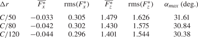
Table 3. Statistics of the tandem configuration,  $H/C = 0.6$, $\phi = 360^\circ$, for different grid sizes.
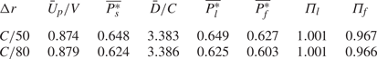
Table 3 shows, for illustration, the effect of the grid spacing on the performance of a tandem case with  $H/C = 0.6$ and $\phi = 360^\circ$. The difference in the propulsive speed from $\Delta r = C/50$ to $\Delta r = C/80$ is less than $1\,\%$ and the difference in the equilibrium distance is $0.003C$, implying that the same tandem configuration is obtained for both grid spacings. The difference in the average power ( $\overline {{P}^*_{i}} \equiv 2 P_i / \rho V^3 S$) is below $4\,\%$; however, when comparing the power ratio, the difference is lower than $0.2\,\%$. Similar results are obtained for the other tandem simulations presented herein.
In view of the results from tables 2 and 3, the simulations are performed with  $\Delta r = C/50$. Only for those configurations where flow visualizations and temporal histories of force and power are presented are the simulations performed with $\Delta r = C/80$.


 Open access