1. Introduction
In the last 15 years, observations with the NASA/Spitzer and ESA/Herschel space telescopes have driven great progress in our understanding of galaxy formation and evolution. It is now clear that the bulk of the super-massive black hole (SMBH) accretion and star formation (SF) in galaxies occurred in the redshift range 1 ≲ z ≲ 3 (Merloni & Heinz Reference Merloni and Heinz2008; Delvecchio et al. Reference Delvecchio2014; Madau & Dickinson Reference Madau and Dickinson2014), and that the galaxy evolution, unlike dark matter structure formation, developed in a ‘top–down’ fashion, with the most massive galaxies and Active Galactic Nuclei (AGNs) forming first (‘cosmic downsizing’). The nearly ubiquitous presence of SMBHs at the centres of galaxies and the close relationship between their masses and the properties of the spheroidal stellar components (Ferrarese & Ford Reference Ferrarese and Ford2005; Kormendy & Ho Reference Kormendy and Ho2013) point to a strong interaction between the build-up of mass in stars and black hole (BH) growth. Nonetheless, the details of these interactions, their impact on cosmic downsizing, and the physical processes that govern SF in galaxies are still largely unclear.
Since the most active cosmic star-formation phases and the associated AGN growth are dust enshrouded, far-infrared (FIR) and sub-millimeter observations are necessary for their detection and astrophysical characterisation. These are the major goals of next-generation observatories.
Imaging alone is insufficient to reach these goals. For example, disentangling AGN and SF contributions via photometric Spectral Energy Distribution (SED) decomposition proved to be extremely challenging even in the presence of a rich amount of optical, near-infrared, and sub-mm (Herschel) data (i.e. Delvecchio et al. Reference Delvecchio2014; Berta et al. Reference Berta2013). FIR/sub-mm spectroscopy adds key information, as demonstrated by the Infrared Space Observatory, Herschel, and Spitzer, albeit with limited sensitivity.
A giant leap forward will be made possible by the FIR to sub-mm imaging and spectroscopic observations performed by the Origins Space Telescope (OST).Footnote a The OST is an evolving concept for the Far-Infrared Surveyor mission, the subject of one of four science and technology definition studies supported by NASA Headquarters in preparation for the 2020 Astronomy and Astrophysics Decadal Survey. By delivering a three order-of-magnitude gain in sensitivity over previous FIR missions and high angular resolution to mitigate spatial confusion in deep surveys, the OST is being designed to cover large areas of the sky efficiently, enabling searches for rare objects at low and high redshifts.
The Origins Survey Spectrometer (OSS) provides OST’s FIR spectroscopic capabilities and enables the execution of wide and deep surveys that will yield large statistical samples of galaxies up to high z. Two design concepts for OST are summarised by Leisawitz et al. (Reference Leisawitz2018), and the mission will be described in detail in a report to the US National Academies’ Decadal Survey in 2019. The OSS has six wide-band grating spectrometer modules, which combine to cover the full FIR spectral range (25–590 μm) simultaneously, with sensitivity close to the astronomical background limit, taking advantage of new far-IR detector array technologies. Because each grating module couples a slit on the sky with a number of beams of the order of 100,Footnote b and OST is agile, allowing for scans perpendicular to the slit at up to 60 mas s−1, OST will be a powerful spatial-spectral survey machine.
Figure 1 shows the wavelength dependence of the sensitivity of OST with the OSS instrument for two studied telescope concepts. The figure shows 5σ detection limits for surveys of 1 000 h each over areas of 1 and 10 deg2. The wavelength dependence is primarily attributable to varying background intensity and secondarily to instrumental effects. The OST study team considered an off-axis 9.1 m diameter telescope (‘Concept 1’) and a 5.9 m diameter on-axis telescope (‘Concept 2’). For Concept 2 in survey mode, the mapping speed in units of [deg2(10−19 W m−2)2/s], with spectral resolving power R = 300, is estimated to be 1.9 × 10⁻⁵ (25–44 μm), 6.9×10⁻⁵ (42–74 μm), 1.2×10⁻⁴ (71–124 μm), 4.1 × 10⁻⁴ (119–208 μm), 1.0 × 10⁻³ (200–350 μm), and 7.1 × 10⁻⁴ (336–589 μm). Mapping speed is proportional to the telescope’s light collecting area, and the area ratio of the Concept 1 to the Concept 2 telescope is 52 m2 / 25 m2 = 2.08. Thus, the mapping speed for Concept 1 is about twice that of Concept 2. A survey of 1 000 h over an area of 1 deg2 with a 5.9 m telescope implies observing times of 0.58, 1.65, 4.67, 13.1, 37.1, and 106.1 s per beam at the central wavelengths of the 6 bands listed above, respectively. The observing times per beam at fixed total time are proportional to the square of the wavelength and inversely proportional to the total area and to the square of the telescope size.
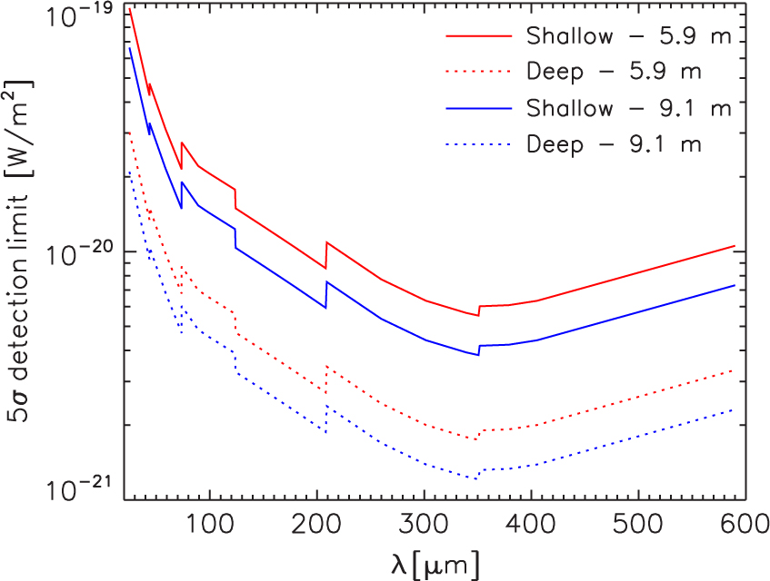
Figure 1. Detection limits of the OSS instrument on OST as a function of wavelength for surveys of 1 000 h each over areas of 1 deg2 (‘deep’) and 10 deg2 (‘shallow’) with 5.9 and 9.1 m telescopes.
The OST will perform unprecedented blind FIR/sub-mm spectroscopic surveys deep and wide enough to provide insight into the physical processes that drive galaxy evolution out to z ∼ 8.5. In the wavelength interval covered by OSS, atomic and molecular lines are present over a broad range of excitation levels for low- and high-z sources. By studying these lines, OST Guest Observers will be able to derive information about the physical conditions and processes active in dust-enshrouded galaxies and AGNs, and measure changes throughout cosmic history.
The detectable IR spectral lines can come from nuclear activity, SF regions, or both. Discriminating between the two contributors is not trivial. However, a key diagnostic stems from the fact that AGNs produce harder radiation and consequently excite metals to higher ionisation states than SF regions. Therefore, lines having high-ionisation potentials are a powerful tool for recognising nuclear activity (Sturm et al. Reference Sturm, Lutz, Verma, Netzer, Sternberg, Moorwood, Oliva and Genzel2002; Meléndez et al. Reference Meléndez2008; Goulding & Alexander Reference Goulding and Alexander2009; Weaver et al. Reference Weaver2010), which may be difficult or impossible to identify via optical spectroscopy in the dusty galaxies with intense SF. Ratios between pairs of lines with different ionisation potentials and comparable critical densities permit the estimation of the gas ionisation state. Ratios between pairs of lines having comparable ionisation potentials and different critical densities allow us to estimate the gas density (Spinoglio & Malkan Reference Spinoglio and Malkan1992). Rubin (Reference Rubin1989) provides a comprehensive discussion of IR density indicators. Sturm et al. (Reference Sturm, Lutz, Verma, Netzer, Sternberg, Moorwood, Oliva and Genzel2002) presented diagnostic diagrams involving different ratios of IR lines (e.g. [Ne vi]7.63/[Ne ii]12.81 vs [Ne vi]7.63/[O iv]25.89), which can be used to identify composite (star-forming plus AGN) galaxies and discriminate between the two components. Other diagnostics exploiting less luminous lines have been presented by Voit (Reference Voit1992b) and Spinoglio & Malkan (Reference Spinoglio and Malkan1992). Given the large number of possible combinations of lines, such diagnostic plots are adaptable to various redshift intervals.
Moreover, the OST with OSS will detect molecular emission lines, in particular CO lines, which are tracers of the physical, chemical, and dynamical conditions in the dense gas typically associated with photo-dissociation regions (PDRs) and the X-ray dominated regions associated with AGNs. The high-J CO lines, detected by Herschel in local galaxies, will be observed with the OST up to high z. Such lines, having high ionisation potentials, are indicators of AGN activity. They are also useful tracers of the physics of the molecular gas. Sub-mm lines are essentially unaffected by dust extinction and can therefore be used to disentangle the contributions from dust enshrouded AGNs and SF in high-redshift galaxies. AGNs and star-forming galaxies (SFGs) have different low- to high-J CO luminosity ratios (see e.g. Carilli & Walter Reference Carilli and Walter2013) due to the different excitation mechanisms and physical conditions (especially temperature and density) in the molecular gas.
In its high-resolution mode, OSS offers velocity resolution ≲ 6.2 km s−1 at 100 μm (Bradford et al. Reference Bradford2018) and will provide information on powerful molecular outflows, with velocities of thousands km s−1. Such outflows are thought to be driven by AGN feedback. As is well known, AGN feedback is a key, but still poorly understood ingredient of most galaxy formation models. A proper study of the outflow detectability requires dedicated, intensive simulations (cf., e.g. González-Alfonso et al. Reference González-Alfonso2017), which are beyond the scope of the present paper.
The OSS on OST will also be able to detect polycyclic aromatic hydrocarbon (PAH) spectral features up to very high redshifts. PAH luminosities are useful indicators of the SF rate (SFR; e.g. Roussel et al. Reference Roussel, Sauvage, Vigroux and Bosma2001; Förster Schreiber et al. Reference Förster Schreiber, Roussel, Sauvage and Charmandaris2004; Peeters, Spoon, & Tielens Reference Peeters, Spoon and Tielens2004; Desai et al. Reference Desai2007; Shipley et al. Reference Shipley, Papovich, Rieke, Brown and Moustakas2016). PAHs were detected in a large sample of galaxies at quite high z (343 ultra-luminous IR galaxies at 0.3 < z < 2.8; Kirkpatrick et al. Reference Kirkpatrick, Pope, Sajina, Roebuck, Yan, Armus, Daíz-Santos and Stierwalt2015), but it is an open question whether PAH features exist in galaxies at higher redshifts. There are indeed indications in the literature of a PAH emission deficit in low-metallicity/low-luminosity SFGs compared to higher-metallicity and/or higher-luminosity SF galaxies (see e.g. Galametz et al. Reference Galametz, Madden, Galliano, Hony and Schuller2009; Rosenberg et al. Reference Rosenberg, Wu, Le Floc’h, Charmandaris, Ashby, Houck, Salzer and Willner2008; Smith et al. Reference Smith, Draine, Dale, Moustakas, Kennicutt and Helou2007; Madden et al. Reference Madden, Galliano, Jones and Sauvage2006; O’Halloran, Satyapal, & Dudik Reference O’Halloran, Satyapal and Dudik2006; Engelbracht et al. Reference Engelbracht, Gordon, Rieke and Werner2005, Reference Engelbracht, Rieke, Gordon, Smith and Werner2008).
The mass-metallicity relation (Tremonti et al. Reference Tremonti2004; Zahid et al. Reference Zahid, Geller, Kewley, Hwang, Fabricant and Kurtz2013) tells us that the metallicity decreases with decreasing stellar mass, and hence with decreasing luminosity. At high z this effect has a stronger impact since the average metallicity decreases with increasing z (Zahid et al. Reference Zahid, Geller, Kewley, Hwang, Fabricant and Kurtz2013). The deficit in PAH emission could be due to greater permeability of dust clouds by PAH-destroying or dissociating interstellar radiation (Galliano et al. Reference Galliano, Madden, Jones, Wilson, Bernard and Le Peintre2003), as low-metallicity clouds are expected to have lower dust-to-gas ratios. PAHs are potentially detectable by the OST/OSS up to z ∼ 8.5, allowing us—for the first time—to shed light on these issues and to analyse the properties of the interstellar medium (ISM) in the early Universe.
Some of the FIR lines detectable by the OST/OSS can be used to measure the metallicity of galaxies. Since the metal abundance results from the cumulative star-formation activity and the gas outflow/inflow history in galaxies, the metallicity of stars and gas in galaxies is an important discriminator between various galaxy evolutionary scenarios. One of the main IR metallicity diagnostics is the ([O iii] 51.81 μm + [O iii] 88.36 μm)/[N iii] 57.32 μm ratio (Nagao et al. Reference Nagao, Maiolino, Marconi and Matsuhara2011; Pereira-Santaella et al. Reference Pereira-Santaella, Rigopoulou, Farrah, Lebouteiller and Li2017). This diagnostic tool is applicable to SFGs and AGNs, and it is almost immune to extinction and insensitive to temperature, density, and the hardness of the radiation field. An additional abundance diagnostic is the ([Ne ii] 12.81 μm + [Ne iii]15.55 μm)/([S iii] 18.71 μm + [S iv] 10.49 μm) ratio (Fernández-Ontiveros et al. Reference Fernández-Ontiveros, Spinoglio, Pereira-Santaella, Malkan, Andreani and Dasyra2016, Reference Fernández-Ontiveros2017). With OSS, OST observers will be able to use these diagnostics to measure the metallicities of hundreds of thousands of galaxies up to z ∼ 6.
In this paper, we adopt the Cai et al. (Reference Cai2013) evolutionary model, as upgraded by Bonato et al. (Reference Bonato2014b). The model was validated by comparison with a broad array of data: multi-frequency (optical, near-IR, mid-IR, FIR, and sub-mm) luminosity functions of galaxies and AGNs at all available redshifts, multi-frequency redshift distributions at several flux density limits, multi-frequency source counts, global and per-redshift slices (Cai et al. Reference Cai2013; Bonato et al. Reference Bonato2014a).Footnote c Appendix A presents comparisons of model predictions with more recent data.
Although there are newer models in the literature (e.g. Guo et al. Reference Guo2016; Lacey et al. Reference Lacey2016; Casey et al. Reference Casey2018), our model is physically grounded and has been tested successfully with the broadest variety of observational data. It also deals self-consistently with the emission of galaxies as a whole, including both the star-formation and the AGN components, with their dependence on galaxy age; this is essential for the purposes of the present paper.
This paper is structured as follows. In Section 2, we present the model. In Section 3, we derive correlations between line and continuum luminosity. In Section 4, we describe our procedure to work out predictions for number counts, IR luminosity functions, and redshift distributions of galaxies and AGNs detectable in the OSS wavelength range. In Section 5, we compare the capabilities of the OST 5.9 and 9.1 m concepts. In Section 6, we investigate in more detail the expected outcome of surveys of different depth with the 5.9 m telescope. In Section 7, we describe the expected scientific impact of the OST/OSS surveys, discuss uncertainties, and compare the OST/OSS performance with that of other FIR/sub-mm instruments. Finally, in Section 8, we summarise our main conclusions.
Throughout this paper, we adopt a flat ΛCDM cosmology with Ωm = 0.31, ΩΛ = 0.69, and h = H 0 / 100 km s−1 Mpc−1 = 0.67 (Planck Collaboration XIII 2016).
2. Outline of the model
In the local Universe, spheroids (i.e. ellipticals and bulges of disk galaxies) are characterised by relatively old stellar populations with mass-weighted ages ≳8–9 Gyr, corresponding to formation redshifts z ≳ 1–1.5, while the disk populations are generally younger. Therefore the progenitors of present day spheroidal galaxies (called proto-spheroids or proto-spheroidal galaxies) are the dominant star forming population at z ≳ 1.5, whereas the SF at z ≲ 1.5 occurs mainly in galaxy disks.
There is a clear evidence of a co-evolution of proto-spheroids and of AGNs hosted by them. Their nuclear activity continues for a relatively short time, of the order of 108 yr, after SF is quenched. At later times, the central SMBHs remain mostly inactive, except for occasional ‘rejuvenations’ due to interactions or mergers. The late nuclear activity is mostly associated with S0’s and spirals, which contain substantial amounts of ISM that can eventually flow towards the nucleus and be accreted.
To deal with these different evolutionary paths, our reference model (Cai et al. Reference Cai2013; Bonato et al. Reference Bonato2014b) adopts a ‘hybrid’ approach. It provides a physically grounded description of the redshift-dependent co-evolution of the SFR of spheroidal galaxies and of the accretion rate onto the SMBHs at their centres, while the description of the evolution of late-type galaxies and of AGNs associated with them is phenomenological and parametric.
The model considers two subpopulations of late-type galaxies: ‘warm’ (starburst) and ‘cold’ (normal) galaxies. While in the case of spheroids, the original model by Cai et al. (Reference Cai2013) dealt simultaneously with the stellar and AGN components, AGNs associated with late-type galaxies were evolved as a separate population. Bonato et al. (Reference Bonato2014b) have upgraded the model to allow for co-evolution of late-type galaxies and their AGNs. This was done by exploiting the mean relation between SFR and accretion rate derived by Chen et al. (Reference Chen2013), taking into account the dispersion around it. The relative abundances of type 1 and type 2 AGNs, as a function of luminosity, were taken into account following Hasinger (Reference Hasinger2008). Bright, optically selected QSOs (for which the Chen et al. Reference Chen2013 correlation is not applicable) are taken into account by adopting the best fit evolutionary model by Croom et al. (Reference Croom2009) up to z = 2 (optical AGNs at higher z are already included in the Cai et al. Reference Cai2013 model). This approach reproduces the observed bolometric luminosity functions of AGNs at different z (see Bonato et al. Reference Bonato2014b).
Table 1. Mean values of the log of line-to-IR (8–1 000 μm) continuum luminosities of galaxies,. 〈log(L ℓ / L IR)〉, and associated dispersions σ. For the PAH 3.3 m, PAH 11.3 μm, and PAH 12.7 μm bands and the H2 17.03 μm, [O i] 63.18 μm, and [C ii] 157.7 μm lines,. 〈log(L ℓ / L IR)〉 has been computed excluding local UltraLuminous Infrared Galaxies (ULIRGs), for which the line luminosity appears to be uncorrelated with L IR. For the latter objects, the last column gives the mean values of log(L ℓ/L⊙) and their dispersions.
1 Taken from Bonato et al. (Reference Bonato2014a)
2 Taken from Bonato et al. (Reference Bonato2014b)
3 Taken from Bonato et al. (Reference Bonato2015)
4 Taken from Bonato et al. (Reference Bonato2017b)
3. Correlations between continuum and line luminosity
To estimate the number of AGN and galaxy line detections achievable with OST/OSS surveys, we coupled the SFR/IR luminosity functions (for the galaxies) or the bolometric luminosity functions (for the AGNs) of each population, as given by the model, with relationships between line and IRFootnote d or bolometric luminosities.
We used the calibrations derived by Bonato et al. (2014a,b, 2015, 2017b) for 31 IR fine-structure lines and the 6 PAH bands at 3.3, 6.2, 7.7, 8.6, 11.3, and 12.7 μm, as they will be accessible in the OST/OSS wavelength range.
The 31 IR fine-structure lines are:
1 coronal region line: [Si vii] 6.50 μm;
8 AGN fine-structure emission lines: [Ne vi] 7.65, [Ar v] 7.90, [Ca v] 11.48, [Ar v] 13.09, [Mg v] 13.50, [Ne v] 14.32, [Ne v] 24.31, and [O iv] 25.89 μm;
13 stellar/H ii region lines: [Ar ii] 6.98, [Ar iii] 8.99, [S iv] 10.49, HI 12.37, [Ne ii] 12.81, [Cl ii] 14.38, [Ne iii] 15.55, [S iii] 18.71, [Ar iii] 21.82, [S iii] 33.48, [O iii] 51.81, [N iii] 57.32, and [N ii] 121.9 μm;
5 lines from PDRs: [Fe ii] 17.93, [Fe iii] 22.90, [Fe ii] 25.98, [Si ii] 34.82, and [O i] 145.5 μm;
4 molecular hydrogen lines: H2 6.91, H2 9.66, H2 12.28, and H2 17.03 μm.
We recalibrated the [O i] 63.18 and [C ii] 157.7 μm PDR lines and the [O iii] 88.36 μm stellar/H ii region line (whose line vs IR luminosity correlations were given in Bonato et al. Reference Bonato2014a), and added more recent data. For these three lines, in addition to the compilation by Bonato et al. (Reference Bonato2014a), we used the data taken from: George (Reference George2015), for all three lines; Brisbin et al. (Reference Brisbin, Ferkinhoff, Nikola, Parshley, Stacey, Spoon, Hailey-Dunsheath and Verma2015) and Farrah et al. (Reference Farrah2013), for the [O i] 63.18 and [C ii] 157.7 μm lines; and Oteo et al. (Reference Oteo2016), Gullberg et al. (Reference Gullberg2015), Schaerer et al. (Reference Schaerer2015), Yun et al. (Reference Yun2015), and Magdis et al. (Reference Magdis2014), for the [C ii] 157.7 μm line only. We excluded all objects for which there is an evidence of a substantial AGN contribution, as was done in our previous work.
The line and continuum measurements of strongly lensed galaxies given by George (Reference George2015) were corrected using the gravitational magnifications, μ, estimated by Ferkinhoff et al. (Reference Ferkinhoff2014), while those by Gullberg et al. (Reference Gullberg2015) were corrected using the magnification estimates from Hezaveh et al. (Reference Hezaveh2013) and Spilker et al. (Reference Spilker2016), available for 17 out of the 20 sources; for the other three sources we used the median value μmedian = 7.4.
For these three lines, Figure 2 shows the correlations between line and IR luminosity. In this plot, the galaxies are subdivided into three groups: local SFGs (L IR < 1012 L⊙, represented by yellow circles), local ULIRGs (L IR ≥ 1012 L⊙, orange triangles), and high-z SFGs (blue squares).

Figure 2. Luminosity of the [O i] 63.18 μm (left panel), [O iii] 88.36 μm (central panel), and [C ii] 157.7 μm (right panel) lines, versus continuum IR luminosity. The green bands show the 2σ range around the mean relation log(L ℓ / L⊙) = log(L IR / L⊙)+c for local SFGs with L IR ≥ 1012 L⊙ (yellow circles) and high-redshift SFGs (blue squares); the values of c ≡ 〈log(Lℓ / L IR)〉 are given in Table 1. The azure bands show the 2σ spread around the mean line luminosity for the sample of local ULIRGs (L IR ≥ 1012 L⊙; orange triangles) whose line luminosities appear to be uncorrelated with L IR and are generally lower than expected from the linear relation holding for the other sources. The mean line luminosities 〈log(L ℓ / L ⊙)〉 of these objects are given in Table 1 as well. See text for the sources of data points.
We warn the reader that the high-z measurements of the three lines mostly refer to strongly lensed galaxies and are therefore affected by the substantial and hard to quantify uncertainty on the correction for magnification, in addition to measurement errors. Not only are estimates of μ for these objects generally poorly constrained by the available data, but they do not necessarily apply to the line emitting gas, which may have a different spatial distribution than the emission used to build the lensing model (differential lensing; Serjeant Reference Serjeant2012). It is, however, reassuring that high-z galaxies do not substantially deviate, on average, from the relations defined by the low-z galaxies.
As noted by Bonato et al. (Reference Bonato2014a), luminosities of the [O i] 63.18 and [C ii] 157.7 μm lines in local ULIRGs do not show any significant correlation with L IR. For such objects we adopted a Gaussian distribution of the logarithm of the line luminosity, log(L ℓ), around its mean value (azure band in Figure 2). Line luminosities of the other populations (low-z non-ULIRGs and high-z SFGs) are consistent with a direct proportionality between log(L ℓ) and log(L IR), i.e. 〈log(L ℓ / L IR)〉 = c ± Δc, represented by the green bands in Figures 2, 3, and 4.Footnote e The mean values and the dispersions are listed in Table 1.
IR luminosities given over rest-frame wavelength ranges different from the one adopted here (8–1 000 μm) were corrected using the following relations, given by Stacey et al. (Reference Stacey, Hailey-Dunsheath, Ferkinhoff, Nikola, Parshley, Benford, Staguhn and Fiolet2010) and Graciá-Carpio et al. (Reference Graciá-Carpio, García-Burillo, Planesas, Fuente and Usero2008), respectively:
 $$L_{{\rm{FIR}}} (40 - 500{\kern 1pt} {\kern 1pt} {\rm{m}}) = 1.5 \times L_{{\rm{FIR}}} (42 - 122{\kern 1pt} {\kern 1pt} {\rm{\mu m}}),$$(1)
 $$L_{{\rm{IR}}} (8 - 1000{\kern 1pt} {\kern 1pt} {\rm{m}}) = 1.3 \times L_{{\rm{FIR}}} (40 - 500{\kern 1pt} {\kern 1pt} {\rm{\mu m}}).$$(2)
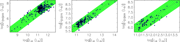
To this initial set of lines, we added the [N ii] 205.2 μm stellar/H ii region line and the [C i] 370.4 and [C i] 609.1 μm PDR lines. We collected data on SFGs from: Lu et al. (Reference Lu2017), Rosenberg et al. (Reference Rosenberg2015), and Walter et al. (Reference Walter, Weiß, Downes, Decarli and Henkel2011) for the [C i] 370.4 and [C i] 609.1 μm lines; Lu et al. (Reference Lu2017), Herrera-Camus et al. (Reference Herrera-Camus2016), and Zhao et al. (Reference Zhao2013, Reference Zhao2016) for the [N ii] 205.2 μm line. In Figure 3, we show the correlations between line and IR emission for these lines. The best-fit values for a direct proportionality and the associated dispersions are listed in Table 1.
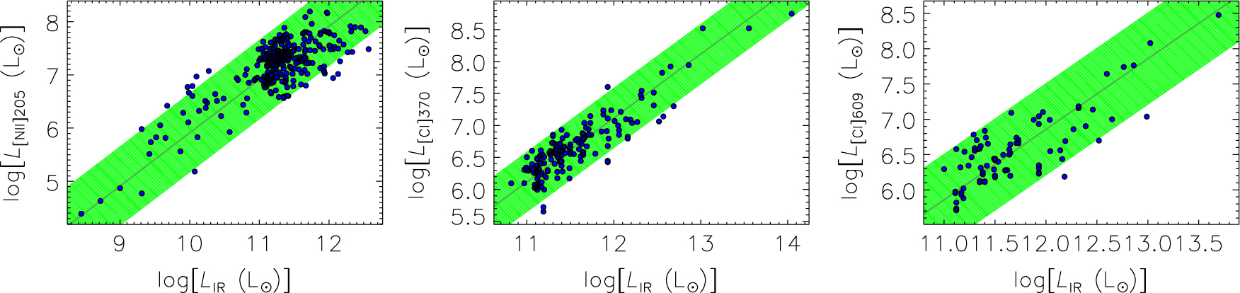
Figure 3. Luminosity of the [N ii] 205.2 μm (left panel), [C i] 370.4 μm (central panel), and [C i] 609.1 μm (right panel) lines, versus continuum IR luminosity. The green bands show the 2σ range around the mean linear relation log(L ℓ / L⊙) = log(L IR / L⊙)+c; the values of c ≡ 〈log(L ℓ / L IR)〉 are given in Table 1. See text for the sources of data points.
For AGNs, empirical correlations between line and bolometric luminosities for 11 IR lines in our sample (specifically, the H2 9.66, [S iv] 10.49, H2 12.28, [Ne ii] 12.81, [Ne v] 14.32, [Ne iii] 15.55, H2 17.03, [S iii] 18.71, [Ne v] 24.31, [O iv] 25.89, and [S iii] 33.48 μm lines) were derived by Bonato et al. (Reference Bonato2014b).
Bonato et al. (Reference Bonato2015) used the IDL Tool for Emission-line Ratio Analysis (ITERA)Footnote f to calibrate the line-to-bolometric luminosity relations for 16 additional AGN IR lines with insufficient observational data ([Si vii] 6.50, H2 6.91, [Ar ii] 6.98, [Ne vi] 7.63, [Ar v] 7.90, [Ar iii] 8.99, [Ca v] 11.48, HI 12.37, [Ar v] 13.09, [Mg v] 13.50, [Cl ii] 14.38, [Fe ii] 17.93, [Ar iii] 21.82, [Fe iii]22.90, [Fe ii] 25.98, and [Si ii] 34.82 μm). These calibrations were found to be in excellent agreement with the available data.
We followed the same procedure to calibrate the line-to-bolometric luminosity relations for the remaining 10 AGN atomic spectral lines in our sample. The AGN contributions to the [N iii] 57.32 μm, [N ii] 121.90/205.18 μm, and [C i] 370.42/609.14 μm lines turned out to be negligible. The best-fit coefficients of the linear relations log(L ℓ/L⊙) = a·log(L bol / L⊙) + b and the associated 1σ dispersions for the lines in our sample are listed in Table 2.
Table 2. Coefficients of the best-fit linear relations between line and AGN bolometric luminosities, log (L ℓ / L⊙) = a log (L bol / L⊙)+b, and 1σ dispersions around the mean relations.
1 Taken from Bonato et al. (Reference Bonato2014b)
2 Taken from Bonato et al. (Reference Bonato2015)
Finally, we derived the line-to-IR luminosity relations for 10 CO lines (J = 4 − 3 through J = 13−12), using the measurements of Kamenetzky et al. (Reference Kamenetzky, Rangwala, Glenn, Maloney and Conley2016). For these molecular lines, the data are consistent with both a linear relation and a direct proportionality between log(L line) and log(L IR). We chose a direct proportionality to avoid an unnecessary second parameter, as was done for the atomic lines. These relations are shown in Figure 4, with the corresponding best-fit parameter values listed in Table 1. Note that while the AGN contribution to the high-J CO lines could be significant, the available observational data are not sufficient to support a derivation of the empirical correlation between AGN bolometric and CO line luminosity.
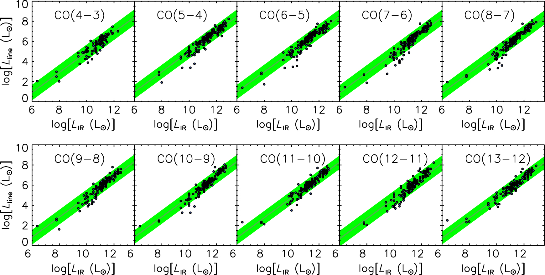
Figure 4. Luminosity of the CO J = 4−3 through J = 13−12 lines versus continuum IR luminosity. The data points are from Kamenetzky et al. (Reference Kamenetzky, Rangwala, Glenn, Maloney and Conley2016). The green band shows the 2σ range around the mean linear relation log(L ℓ / L⊙) = log(L IR / L⊙)+c; the values of c ≡ 〈log(L ℓ / L IR)〉 are given in Table 1.
Similar to what was done in Bonato et al. (Reference Bonato2017b), the detection limits for the broad PAH bands were computed assuming that the spectra are degraded to R = 50 from the original R = 300, resulting in a sensitivity gain by a factor of  $\sqrt 6 $.
4. Number counts and redshift distributions
We computed redshift-dependent line luminosity functions using the Monte Carlo approach described in Bonato et al. (2014a,b). These papers dealt with dust-obscured SF phases, for which L IR is an excellent estimator of the SFR. The line-L IR relations presented in Section 3 were also based on the observations of dusty galaxies, for which the unabsorbed fraction of the UV emission from young stars is small.
However, the OST with OSS will push the observational frontier to lower luminosity, higher redshift galaxies, with higher fractions of unabsorbed UV light, i.e. with smaller fractions of the SFR measured by L IR. The following question then arises: Are the relationships derived above for the case ‘L IR equivalent to SF luminosity’ to be interpreted as relations of line luminosity with SFR, or with L IR?
De Looze et al. (Reference De Looze2014) analysed the reliability of three of the brightest FIR fine-structure lines, [C ii] 157.7 μm, [O i] 63.18 and [O iii] 88.36 μm, to trace the obscured plus unobscured SFR (measured by the FIR and by the UV luminosity, respectively) in a sample of low-metallicity dwarf galaxies from the Herschel Dwarf Galaxy Survey. Furthermore, they extended the analysis to a large sample of galaxies of various types and metallicities taken from the literature. Their results confirmed that the line luminosity primarily correlates with the SFR.
We could not find in the literature any other study on the relation between FIR lines and SFR that took into account both the UV and the FIR luminosity. In general, the SFR is derived from the FIR luminosity. We have therefore assumed that the conclusions by De Looze et al. (Reference De Looze2014) can be extended to all FIR fine structure lines: we do not see any obvious reason why the luminosity of these lines should depend on the fraction of UV radiation absorbed by dust.
The situation is different for the PAH emission because these large molecules may be destroyed by absorption of UV or soft X-ray photons (Voit Reference Voit1992a). They more easily survive if they are shielded by dust. A weakening of PAH emission relative to dust emission at low gas-phase metallicity was reported by Engelbracht et al. (Reference Engelbracht, Gordon, Rieke and Werner2005). Shipley et al. (Reference Shipley, Papovich, Rieke, Brown and Moustakas2016) found that the PAH luminosity correlates linearly with the SFR, as measured by the extinction-corrected H α luminosity, for gas-phase metallicity log Z = 12 + log(O / H) ≥ log Zc = 8.55, but strongly decreases with decreasing Z for Z ≤ Zc. We have adopted their empirical correction for Z ≤ Zc galaxies:
 $$\log L_{{\rm{PAH}},\lambda }^{{\rm{corr}}} = \log L_{{\rm{PAH}},\lambda } + A[\log Z - (\log {\rm{Z}}_ \odot - \log Z_0 )],$$(3)
where LPAH ,λ is the luminosity of the PAH band at the wavelength λ derived from the IR luminosity, taken as a measure of the SFR (Section 3), A is given, for different PAH bands, by Table 4 of Shipley et al. (Reference Shipley, Papovich, Rieke, Brown and Moustakas2016), and log Z 0 = log Z ⊙ − 8.55 = 0.14. For the conversion from L IR to SFR we have adopted the calibration by Kennicutt & Evans (Reference Kennicutt and Evans2012):
 $$\log ({\kern 1pt} {\rm{SFR}}{\kern 1pt} /{\rm{M}}_ \odot {\kern 1pt} {\kern 1pt} {\rm{yr}}{\kern 1pt} ^{ - 1} ) = \log (L_{{\rm{IR}}} /{\rm{L}}_ \odot ) - 9.82.$$(4)
A relation between metallicity, SFR, and stellar mass, M ⋆, approximately independent of redshift, was found by Hunt et al. (Reference Hunt, Dayal, Magrini and Ferrara2016):
 $$12 + \log (O/H) = - 0.14 \log ({\kern 1pt} {\rm{SFR}}{\kern 1pt} ) + 0.37\log (M_ \star ) + 4.82.$$(5)
Finally, a redshift-dependent relationship between M ⋆ and SFR was derived by Aversa et al. (Reference Aversa, Lapi, de Zotti, Shankar and Danese2015) using the abundance-matching technique. We have exploited this set of equations to account for the metallicity dependence of the PAH luminosity.
The molecular lines are even more complex. Two main issues are at play: the relationship between SFR and molecular gas density (essentially the Schmidt–Kennicutt law; Kennicutt Reference Kennicutt1998), whose shape is still debated, and the uncertain CO-to-H 2 conversion factor (Bolatto, Wolfire, & Leroy Reference Bolatto, Wolfire and Leroy2013). A strong decrease of the CO luminosity to SFR at low metallicity has long been predicted as a consequence of the enhanced photo-dissociation of CO by ultraviolet radiation (e.g. Bolatto et al. Reference Bolatto, Wolfire and Leroy2013). Genzel et al. (Reference Genzel2012) and Hunt et al. (Reference Hunt2015) found that a direct proportionality between L CO and SFR, consistent with that reported in Section 3, holds for Z ≳ Z ⊙, while the L CO/SFR ratio drops for lower metallicity. We have adopted the empirical relationship presented by Hunt et al. (Reference Hunt2015) for log log Z ≲ 8.76 (see their Figure 5):
 $$\log L_{{\rm{CO}}}^{{\rm{corr}}} = \log L_{{\rm{CO}}} ({\kern 1pt} {\rm{SFR}}{\kern 1pt} ) + 2.25\log Z - 19.71,$$(6)
where L CO(SFR) is the relationship derived in Section 3, after converting L IR to SFR using Eq. (4). The mean metallicity corresponding to a given SFR was computed as described above.
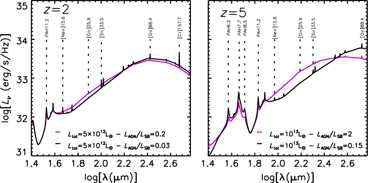
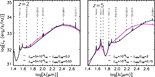
Figure 5. Examples of SEDs with AGN and SF components in the observer frame, over the wavelength range of the OST/OSS (25–590 μm). The SEDs are shown for sources at z = 2 (left) and z = 5 (right) and for the different total source luminosities L tot = L AGN + L IR,SF and L AGN / L IR,SF ratios specified in the inset. All the spectral lines of our sample are included in the SEDs. Some of the brightest lines are labelled.
Clearly, the relationships between the PAH or CO emissions and the SFR (hence our estimates of the corresponding redshift-dependent luminosity functions and number counts) are affected by large uncertainties, especially at high redshifts. FIR spectroscopic surveys conducted with the OST will shed light on these issues.
As in Bonato et al. (Reference Bonato2014b), our simulations take into account both the SF and the AGN components (see Section 2). We calculated line luminosity functions in 100 redshift bins with a width, Δz, of ∼0.08. For each redshift bin, at the bin centre, we extracted from the model SFR/IR luminosity functions (for galaxies) or from the bolometric luminosity functions (for AGNs), a number of objects, brighter than log(L IR,min / L⊙) = 8.0, equal to that expected in 1 deg2.
The luminosities of SF and AGN components of each source were randomly extracted from the probability distributions that an object at redshift z has a starburst luminosity L IR,SF or an AGN luminosity L AGN, given the total luminosity L tot = L IR,SF + L AGN. The probability distributions are given by Bonato et al. (Reference Bonato2014b).
The line luminosities associated with each component were randomly taken from Gaussian distributions with the mean values and dispersions given in Tables 1 and 2. In this way we get, at the same time, luminosities of all the lines of both the SF and AGN components of each simulated object, allowing us to make interesting predictions. For example, we can ask: For how many objects will both components be detectable given the survey sensitivity? How many will be detectable in two or more lines? Figure 5 shows examples of SEDs with AGN and SF components at z = 2 and z = 5.
We derived line luminosity functions by binning the simulated line luminosities within each redshift bin. We repeated the simulations 1 000 times and averaged the derived line luminosity functions. Finally, number counts were derived after assigning to each source a redshift drawn at random from a uniform distribution within the redshift bin and computing the corresponding flux. For more details, see Bonato et al. (Reference Bonato2014b).
5. Comparison between the 5.9 and 9.1 m concepts
The first question we want to address is whether, from the point of view of extragalactic spectroscopic surveys with OST, there is strong scientific motivation to favour the more ambitious Concept 1 (9.1 m telescope), compared to Concept 2 (5.9 m telescope with a central obstruction). With the performances mentioned in Section 1, realistic surveys of different depths could cover areas in the range 1–10 deg2.
5.1. Number counts
The survey depth at fixed observing time scales as the square root of the ratio of the effective light collecting areas of the two concepts, i.e. as (52 m2 / 25 m2)1/2 = 1.44. To quantify the effect of such a difference in depth, we have computed the number of 5 σ line detections in 1 000 h by the OSS with both OST concepts, as a function of the mapped area. The results are shown in Figure 6.
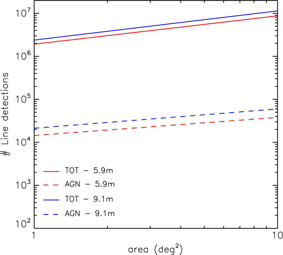
Figure 6. Number of 5σ starburst (solid) and AGN (dashed) line detections as a function of the mapped area, for a survey of 1 000 h.
In all cases, the slopes of the counts are relatively flat at the detection limits, implying that the number of detections in each line increases more with the area than with the depth of the survey. We expect ∼1.9×10⁶ to ∼8.7×10⁶ line detections for the 5.9 m telescope, depending on the survey area, and ∼2.4×10⁶ to ∼1.1×10⁷ for the 9.1 m telescope. The number of detections in pure AGN lines ranges from ∼1.4×10⁴ to ∼3.8×10⁴ for the 5.9 m telescope, depending on the survey area, and from ∼2.1×10⁴ to ∼6.0×10⁴ for the 9.1 m telescope.
We thus conclude that the decrease of the telescope size from 9.1 to 5.9 m does not translate into a substantial worsening of the detection statistics, at least in terms of counts.
5.2. Redshift and luminosity distributions
Of course, a comparison of the total number of detections is not enough to answer the question posed at the beginning of this section, since going deeper may allow us to reach poorly populated but interesting regions of the redshift-luminosity plane.
Figure 7 shows the predicted redshift distributions of sources detectable by OSS in at least one spectral line over an area of 1 deg2 in 1 000 h of observations for both OST mission concepts. Although the larger telescope surpasses the smaller one in source detections, and does so increasingly at greater redshifts, both telescope sizes allow galaxy detections with good statistics up to z ≃ 8, while the statistics are poor in both cases at higher redshifts.
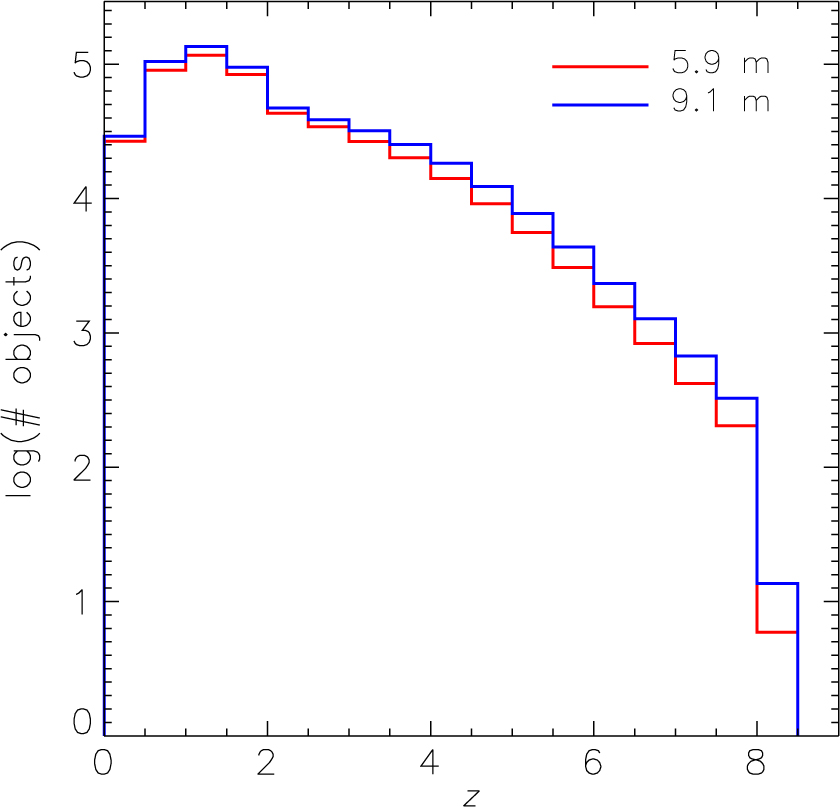
Figure 7. Predicted redshift distributions of galaxies detected with a 5.9 m and a 9.1 m OST spectroscopic survey in 1 000 h of observing time, assuming an areal coverage of 1 deg2.
The advantage of a larger telescope is somewhat greater if the objective is to investigate galaxy-AGN co-evolution, which requires that sources be detectable simultaneously in at least one SF line and one AGN line (Figure 8). At z ≥ 4.5, the 9.1 m telescope detects about twice as many sources as the 5.9 m telescope, but the statistics are limited in both cases at this redshift.
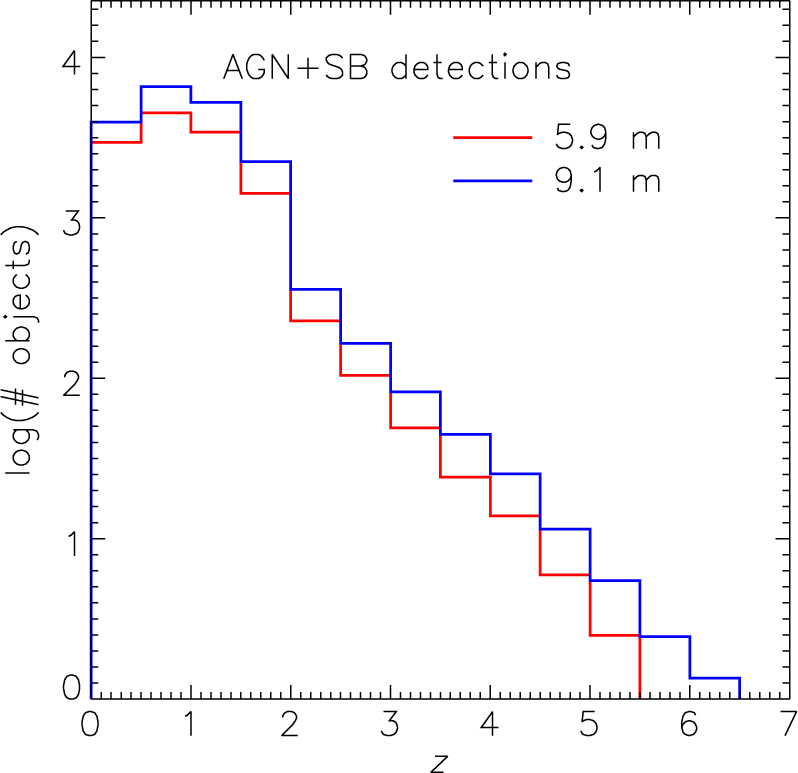
Figure 8. Predicted redshift distributions of galaxies detected simultaneously in at least one SF line and one AGN line with a 5.9 m and a 9.1 m OST spectroscopic survey in 1 000 h of observing time, assuming an areal coverage of 1 deg2. The corresponding AGN redshift distributions are almost identical to these, indicating that whenever the AGN component is detected, the SF component is detected as well.
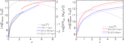
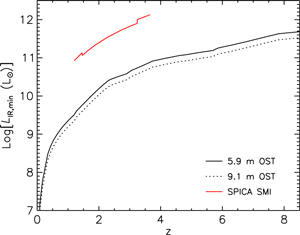
To investigate the effect of telescope size on the determination of the redshift-dependent IR luminosity functions (hence of the SFR functions) and of AGN bolometric luminosity functions, we computed the minimum L IR and the minimum  $ L_{{\rm{bol}}}^{{\rm{AGN}}} $ corresponding to the minimum luminosity of some bright lines detectable in a 1 000 h survey of 1 deg2. To this end, we have used the appropriate value of the mean line-to-IR or bolometric luminosity ratio. The results are shown, as a function of redshift, in Figure 9.
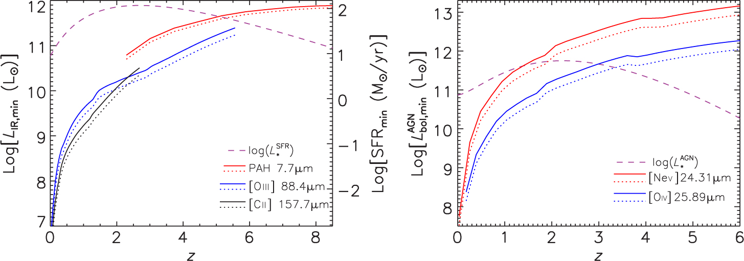
Figure 9. Minimum IR luminosity—SFR (left panel, left and right y-axis respectively) and minimum AGN bolometric luminosity (right panel) detected, as a function of redshift, with a 5.9 m (solid lines) and a 9.1 m (dotted lines) OST survey with an areal coverage of 1 deg2, through spectroscopic detections of key SF and AGN lines. The dashed purple lines show, for comparison, estimates of the redshift-dependent characteristic luminosity, L ⋆, of dusty galaxies and AGNs, respectively (see text).
The luminosities of the chosen SF lines (left panel) are proportional to L IR, so the larger telescope would allow OST observers to reach luminosities lower by a factor of 1.44. In the case of AGN lines, the ratio depends on luminosity, so the advantage of the larger telescope slightly increases with z, reaching a factor of ≃1.7 at z = 6 (right panel).
The right-hand scale on the left panel of Figure 9 shows the SFR corresponding to L IR, as given by Eq. (4). Two points should be noted here. First, as discussed in Section 4, in the case of the PAH lines Eq. (4) breaks down at low metallicities, so the correspondence between L IR derived from the PAH luminosity and the SFR is to be taken with caution, although the effect of metallicity is expected to be minor at the relatively high values of L IR shown here. Second, Eq. (4) holds for a Kroupa stellar IMF. Recent ALMA measurements of multiple CO transitions in four strongly lensed sub-mm galaxies at z ≃ 2−3 (Zhang et al. Reference Zhang, Romano, Ivison, Papadopoulos and Matteucci2018) have provided evidence for a top-heavy IMF, implying a greater fraction of massive stars. Their preferred IMF would translate into a higher L IR / SFR ratio by about 40%.
The dashed purple lines in Figure 9 show, for comparison, estimates of the characteristic luminosity, L ⋆, as a function of redshift, for dusty galaxies and AGNs (left- and right-hand panel, respectively). The plotted values of L ⋆(z) refer to the modified Schechter function defined by Eq. (9) of Aversa et al. (Reference Aversa, Lapi, de Zotti, Shankar and Danese2015). In the case of dusty galaxies, LIR,.min < L ⋆ up to z≃5.9 or z≃6.2 for the 5.9 and the 9 m telescope, respectively. This OST/OSS will then provide a good description of the evolution of the bulk of the IR luminosity function, hence of the IR luminosity density, up to these redshifts. In the AGN case, Lbol,min < L ⋆ up to z≃3 or z≃3.3 for the two telescope sizes.
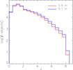
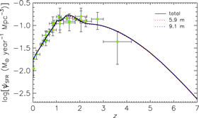
Finally, Figure 10 shows the fractions of the SFR density resolved by the deep spectroscopic surveys as a function of z for the two telescope sizes. The SFR density is almost fully resolved in both cases (≃97% with the 5.9 m concept, ≃98% with the 9.1 m telescope).
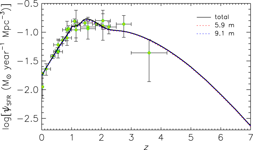
Figure 10. Cosmic SFR density resolved by an OST/OSS deep survey (1 000 h over an area of 1 deg2) with a 5.9 m (dotted red line) or a 9.1 m (dotted blue dotted) telescope, as a function of z. The black solid line shows the total SFR density yielded by our model. The data points are from Madau & Dickinson (Reference Madau and Dickinson2014).
5.3. Confusion
The telescope in both OST concepts is diffraction limited at 30 m. Throughout most of the OSS wavelength range, a larger telescope provides better angular resolution and will be less prone to spatial confusion. Is source confusion an issue, especially for the 5.9 m telescope? Since spectroscopy adds a third dimension, confusion is in general far less significant than would be the case for a continuum survey. In spectroscopy, confusion arises if lines from different sources along the line of sight can show up by chance in the same spectral and spatial resolution element.
Figure 11 shows the total integral number counts of lines per beamFootnote g and per spectral resolution element at different wavelengths within the OST/OSS spectral coverage, for the 5.9 and 9.1 m telescope concepts. The line detection limits for a deep survey of 1 deg2 are represented by the vertical dashed lines. Even in the worst case (longest wavelength and smaller telescope size), the source density per resolution element is <1/22, i.e. the confusion is only marginal, and observations at shorter wavelengths, where the detection limits are well above the confusion limit, will help to resolve confusion in three (spatial-spectral) dimensions. Thus, line confusion is never an issue for the 9.1 m telescope and realistic exposure times. The 5.9 m telescope option can hit the confusion limits only at the longest wavelengths, and only for very deep surveys (≥1000h over 1 deg2).
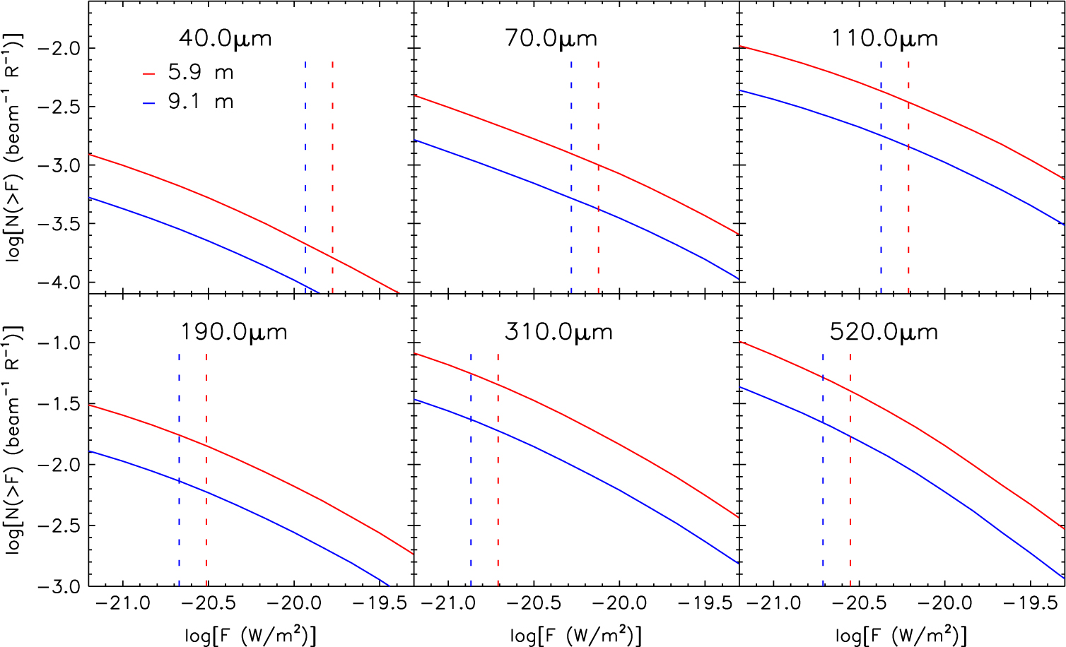
Figure 11. Total integral line number counts per beam and per spectral resolution element at different wavelengths within the OST/OSS spectral coverage for the 5.9 m (red) and the 9.1 m (blue) telescopes. The vertical dashed lines represent the detection limits for surveys of 1 000 h covering 1 deg2.
6. Surveys with the 5.9 m OST
The analysis presented in the previous section has not exposed any scientifically compelling advantage of the 9.1 m telescope over the 5.9 m telescope. In this section, we focus on the latter option and compare in more detail the outcome of surveys covering different areas at fixed total observing time, considering the cases of a wide and shallow (10 deg2 area) and a deep (1 deg2) survey, each conducted in an observing time of 1 000 h.
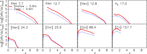
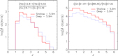
In Figure 12 we display the redshift distributions of galaxies observed in the three brightest AGN lines ([Ne v]14.32, [Ne v]24.31, and [O iv]25.89 μm) and in some of the most often detected SF indicators. Obviously, only the shortest wavelength lines can be detected up to very high redshifts. The figure clearly shows that the OST is so sensitive that even the shallow survey can reach the highest redshifts. Again, the number of detections increases more with increasing survey area than with increasing depth. Hence, the shallow survey yields better statistics than the deep one, except at the highest redshifts, and only for certain lines. Even in the most favourable cases, the deep survey offers only minor advantages from a statistical perspective.
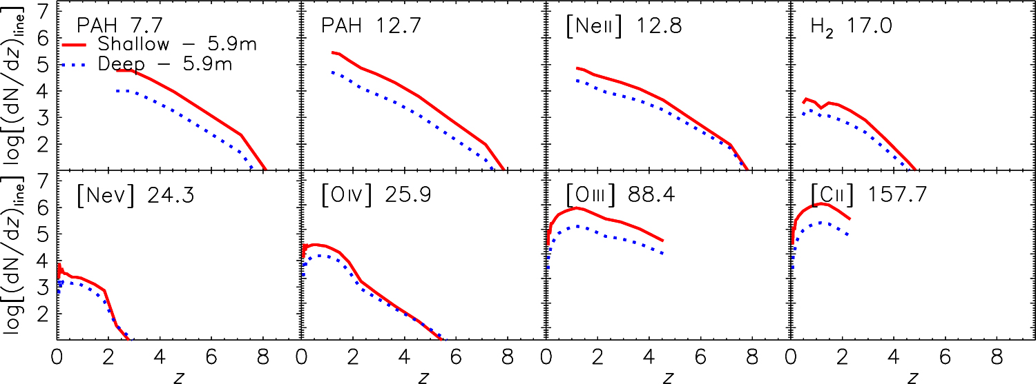
Figure 12. Predicted redshift distributions of galaxies detected in the three brightest AGN lines ([Ne v]14.32, [Ne v]24.31, and [O iv]25.89 μm) and in selected lines indicating SF, namely those with relatively high detection rates. The predicted distributions pertain to shallow (solid red lines, 10 deg2 areal coverage) and deep (dotted blue lines, 1 deg2 areal coverage) surveys, each conducted in 1 000 h of observing time with a 5.9 m telescope.
A factor of 10 decrease in the surveyed area at fixed total observing time translates into a decrease in the minimum detectable line luminosity at given z by a factor of 101/2≃3.16. In the case of the fine structure lines, such as [Ne ii] 12.8 μm (upper panels of Figure 13), which are estimators of the total (dust obscured and unobscured) SFR, going deeper simply means extending the luminosity function to fainter levels. In the case of the [Ne ii] 12.8 μm line, the ratios of numbers of detections per unit area between the deep and the shallow surveys are ≃3.2 and 7.5 at z = 3 and z = 7, respectively, for a 5.9 m telescope. These ratios do not compensate for the factor of 10 difference in survey area, so the total number of detections is larger for the wide, shallow survey.
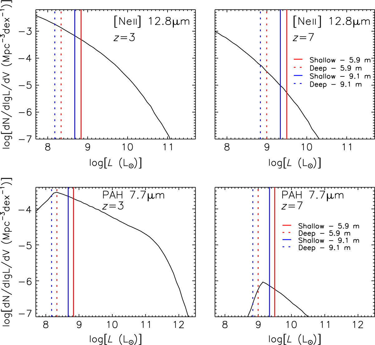
Figure 13. Luminosity functions of the fine structure line [Ne ii] 12.8 μm (upper panels) and the PAH 7.7 μm line at z = 3 and z = 7. The decline of the faint end of the PAH luminosity function is due to the effect of decreasing metallicity.
In the case of PAH lines, the minimum detectable luminosity is in the range where their emission is substantially reduced due to a decrease in metallicity, as discussed in Section 4, and a corresponding dip is seen at the low-luminosity end of the PAH luminosity function. Hence, the increase in the number of PAH detections per unit area with decreasing detection limit is rather modest. For example, the ratio of the number of detections of the 7.7 μm line between the deep and shallow surveys is ≃1.7 at z = 3 and ≃2.1 at z = 6 (lower panels of Figure 13). The increase in the total number of detections per unit area is also small since PAHs are the dominant contributors. On the other hand, this luminosity range carries information about the poorly known dependence of L IR on metallicity and on the impact of varying metallicity on the PAH emission.
According to our model, the brightest IR AGN line, [O iv] 25.89 μm, will be detected in ∼33000 sources by the shallow survey and in ∼12000 sources by the deep one, reaching, in both cases, z ∼5.5. The shallow survey will yield about 750 000 PAH detections up to z ∼8.5, the deep survey about 135 000 up to z ∼7.5. The counter-intuitive decrease in the maximum redshift with increasing survey depth, at fixed observing time, is due to the increasing scarcity of bright PAH lines at high z, a consequence of decreasing metallicity: large-area surveys are needed to find rare sources.
The [C ii] 157.70 μm line, the strongest line emitted by the cool gas in galaxies (<104 K; see Carilli & Walter Reference Carilli and Walter2013), is detectable up to z ∼3.2 by the two surveys. We predict that the line will be seen in about 1.6 million galaxies by the shallow survey and in ∼280000 galaxies by the deep survey. Moreover, the shallow and deep surveys will yield ∼12300 and ∼4500 detections, respectively, up to z ∼ 5, in the four warm H2 lines, which are good diagnostics of the turbulent gas (upper right-hand panel of Figure 12).
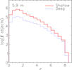
The conclusion that there is no need for exposures longer than those of the shallow survey to reach the highest redshifts is confirmed by Figure 14, which illustrates the global redshift distributions of sources detectable with the two notional surveys. The shallow survey will detect ∼2.7×10⁶ galaxies, while the deep survey will detect ∼4.8×10⁵. The peak of the distributions is at z∼1.5, close to the peak of SF and BH accretion activity. The shallow and deep surveys will detect about 31 000 and about 12 000 galaxies at z >5, respectively.
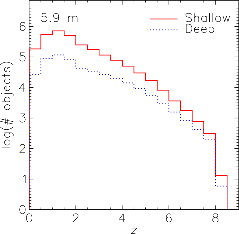
Figure 14. Predicted global redshift distributions of galaxies detected in spectral lines by the shallow (10 deg2) and deep (1 deg2) surveys with a 5.9 m telescope. Each survey has a total amount of observing time equal to 1 000 h.
For the fixed amount of observing time considered, the deep survey does not offer any significant advantage over the shallow survey, even if we are looking for sources detected simultaneously in at least one SF line and one AGN line. Figure 15 shows that the deep survey detects more such objects only at z >5, but even there the difference is small and the statistics are poor. The total number of detections of such high-z sources are of ∼3.4×10⁴ and ∼1.3×10⁴ for the shallow and deep surveys, respectively.
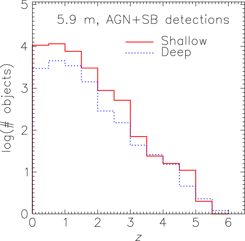
Figure 15. Predicted redshift distributions of galaxies detected simultaneously in at least one SF line and one AGN line by the deep (1 deg2) and shallow (10 deg2) surveys with a 5.9 m telescope. Both surveys have a total amount of observing time equal to 1 000 h. As in the case of Figure 8, these distributions are almost identical to the redshift distributions of AGNs detected by the two surveys.
Next consider the two metallicity diagnostics described in Section 1, involving the following spectral lines: (1) [Ne ii] 12.81, [Ne iii] 15.55, [S iii] 18.71, and [S iv] 10.49 μm; or (2) [O iii] 51.81, [O iii] 88.36, and [N iii] 57.32 μm. Figure 16 shows the redshift distributions of sources detectable by the shallow and deep surveys conducted with a 5.9 m telescope in 1 000 h of observing time, for which these two metallicity diagnostics can be built, thanks to the simultaneous detection of the two sets of lines.
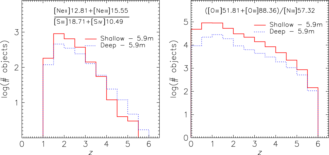
Figure 16. Left panel: predicted redshift distributions of galaxies detected simultaneously in the [Ne ii] 12.81, [Ne iii] 15.55, [S iii] 18.71, and [S iv] 10.49 μm lines by the shallow (10 deg2) and deep (1 deg2) surveys with a 5.9 m telescope. Both surveys have a total amount of observing time equal to 1 000 h. Right panel: the same, but for the simultaneous detection of the [O iii] 51.81, [O iii] 88.36, and [N iii] 57.32 μm lines.
The deep survey is advantageous for the first metallicity diagnostic at z >4, although the total number of detections is larger for the shallow survey (∼2300 vs ∼1400). In the case of the second metallicity diagnostic, the shallow survey is better at all redshifts: the total number of detections is ≃3.6×10⁵ with ∼1000 galaxies at z >5, versus ≃1.0×10⁵ with ∼600 galaxies at z >5 for the deep survey.
7. Discussion
7.1. Galaxy-AGN co-evolution
As shown in Figure 8, we predict the simultaneous detection of SF and AGN lines for a large sample (a few tens of thousands) of galaxies. The brightest IR AGN line—[O iv] 25.89 μm—will allow us to estimate the bolometric luminosity of the AGN component of the sources up to z ∼ 5.5−6, while starburst lines provide estimates of the IR luminosity, and hence the SFR up to z ∼ 8−8.5 (Figure 12). In other words, for the first time OST will enable observers to explore the physical processes driving galaxy-AGN (co-)evolution throughout most of cosmic history, with excellent statistics.
Figure 17 illustrates the extent to which galaxy-AGN co-evolution can be tested with OSS spectroscopy at three redshifts (z = 2, 3, and 5) around and beyond the peak of SF and BH accretion activity. The figure shows, as a function of area mapped, the minimum ratio of the AGN bolometric luminosity, L AGN, to the IR luminosity, L IR ≡ L IR,SF, of the host galaxy for which OST can detect both the [O iv] 25.89 μm and the [O iii] 88.36 μm lines. As shown above, these lines are good indicators of the AGN and SF luminosities, respectively. The curves refer to five values of the total bolometric luminosity, L tot = L AGN +L IR,SF, of the source,Footnote h ranging from 5×10¹¹ to 5×10¹³ L⊙.Footnote i
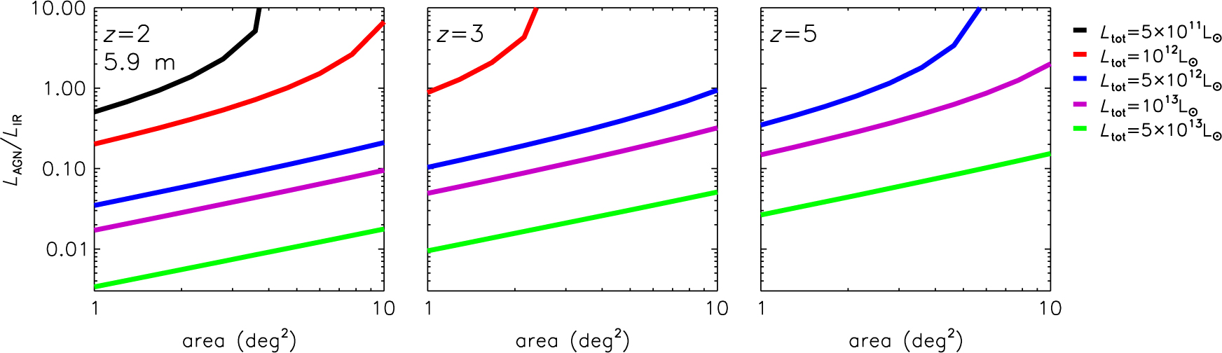
Figure 17. Minimum ratios of AGN bolometric luminosities to SF IR luminosity L IR ≡ L IR,SF for which lines associated with both components (the [O iv] 25.89 μm and the [O iii] 88.36 μm lines, respectively) are detectable with the OST/OSS at z = 2 (left), z = 3 (centre), and z = 5 (right), as a function of the mapped area for five values of L tot = L AGN +L IR,SF.
During the dust-obscured intense SF phase, the BH is expected to accrete at, or perhaps slightly above, the Eddington limit. At the end of this phase, its mass should, on average, be close to that given by the correlations with host galaxy properties. The corresponding AGN bolometric luminosity, L AGN, can be about an order of magnitude greater than the IR luminosity of the host galaxy, L IR,SF. For a source with L tot = 1013 L⊙, the deep survey (1 deg2) could detect both AGN and SF lines down to L AGN / L IR,SF≃0.017 at z = 2, ≃0.05 at z = 3, and ≃0.15 at. z = 5.
For Eddington-limited accretion, the corresponding BH masses are ≃5.2×10⁶ M⊙, ≃1.5×10⁷ M⊙, and ≃4.1×10⁷ M⊙ at redshifts 2, 3, and 5, respectively. The final total luminosity of these objects is AGN dominated; using the Cai et al. (Reference Cai2013) Eddington ratios, we find that the final BH masses are 3.1×10⁸ M⊙, 2.6×10⁸ M⊙, and 1.4×10⁸ M⊙, respectively. Thus the OST/OSS surveys can detect AGNs when their BH masses are factors ∼60 (at z≃2), ∼18 (at z≃3), and ∼3 (at z≃5) lower than the final values, for a galaxy with a total IR luminosity of 1013 L⊙. The probed BH mass growth range will be larger for the rare more luminous sources. Thus, the [O iv] 25.89 μm line, which is not much affected by dust obscuration, is an efficient tool for taking a census of faint AGNs inside dusty SFGs.
Existing information on co-evolution is very limited and based on a combination of X-ray and far-IR/sub-mm data. X-ray observations are currently the most efficient way to reliably identify AGNs. However, X-ray emission associated with stellar processes can reach luminosities of ≃1042 erg s−1 (cf., e.g. Lehmer et al. Reference Lehmer2016), and this makes the identification of lower luminosity AGNs challenging or impossible. OST observations will not have this limitation; OST will be able to detect less luminous AGNs in the local Universe.
For example, using an X-ray bolometric correction of 20, as appropriate at the luminosities considered (Lusso et al. Reference Lusso2012), we find that an OST (5.9 m) deep survey with OSS can detect AGN line signatures via the [O iv] 25.89 μm line up to a factor of ∼12 fainter at z ≃ 0.2. The redshift distribution of galaxies detected simultaneously in at least one SF line and one AGN line (Figure 15) implies that the OST will detect the AGN component of about 3 500 galaxies at z ≤ 0.2.
Alternative methods to detect faint AGNs include sub-arcsec mid-IR imaging to isolate the AGN component from the emission due to SF (currently possible only for nearby AGNs; e.g. Asmus et al. Reference Asmus, Gandhi, Hönig, Smette and Duschl2015), and mid-IR photometry in the wavelength range 3–30 μm (e.g. Assef et al. Reference Assef2013). The latter approach exploits the fact that the AGN emission is ‘hotter’ than that due to SF to decompose the observed spectral energy distribution, separating the two components; it works primarily for intrinsically luminous but heavily obscured AGNs.
Current studies of the connection between AGN activity and SF have been carried out using either the X-ray emission of SFGs (e.g. Delvecchio et al. Reference Delvecchio2015) or the SF properties of X-ray selected AGNs (e.g. Stanley et al. Reference Stanley, Harrison, Alexander, Swinbank, Aird, Del Moro, Hickox and Mullaney2015). In both cases, caveats apply to the interpretation of the results. X-ray detections were found in only a small fraction of the SFGs selected from Herschel surveys. For example, only about 10% of galaxies in the Delvecchio et al. (Reference Delvecchio2015) sample were detected in X-rays. For the overwhelming majority of galaxies, only average AGN accretion rates (or bolometric luminosities) could be determined by stacking. The X-ray selected sample by Stanley et al. (Reference Stanley, Harrison, Alexander, Swinbank, Aird, Del Moro, Hickox and Mullaney2015) has the opposite problem: only upper limits to the IR luminosity due to SF could be placed for 75.4% of the sources. In both cases, a large fraction of objects have only photometric redshift estimates. Spectroscopic redshifts are available for 53% of the Stanley et al. (Reference Stanley, Harrison, Alexander, Swinbank, Aird, Del Moro, Hickox and Mullaney2015) sample, while for the one by Delvecchio et al. (Reference Delvecchio2015) the fraction of spectroscopic redshifts is ≃60% at z ≤ 1.5, but drops to 20% at z≃2. For comparison, the proposed OST/OSS surveys will detect both SF and AGN spectral signatures for tens of thousands of sources up to z∼5.5−6.
7.2. Evolution of gas metallicity
Detection of the bright PAH bands up to z∼8.5 will allow us, for the first time, to follow their entire history up to the reionisation epoch, and therefore to explore the properties of the ISM and to address many open questions regarding their formation, destruction, and dependence on metallicity.
Most galaxies will be detected by the OST/OSS in at least 2 lines (∼60% of the galaxies observed with the 5.9 m OST shallow survey and ∼70% with the deep survey). Therefore, we will have robust spectroscopic redshift measurements. Figure 16 shows that the OST will allow us to measure metallicity in galaxies up to to z∼6.
The results presented in this paper pertain to blind surveys. Obviously, the OST/OSS could go deeper by targeting known high-z galaxies, but blind, unbiased surveys are needed to obtain unbiased censuses of the SFR density and the BH accretion rate density.
7.3. Caveats
Although our reference model was validated against a wide variety of data, it necessarily relies on a number of simplifying assumptions and, as any other model, cannot match the enormous variety of individual galaxy and AGN properties.
Recent observations (Dowell et al. Reference Dowell2014; Asboth et al. Reference Asboth2016; Ivison et al. Reference Ivison2016) have yielded estimates of the space density of distant (z ≳ 4) dusty SFGs well in excess of model predictions. As shown in the Appendix, the model matches quite well the redshift distribution of such sources estimated by Ivison et al. (Reference Ivison2016), but underestimates by a factor of ≃2.5 their (highly uncertain) total counts.
The interpretation and even the reality of the excess are still unclear (Béthermin et al. Reference Béthermin2017; Donevski et al. Reference Donevski2018). If real, the excess would imply that the OST will detect several times more high-z galaxies. Note that most redshift estimates used to search for high-z galaxies are photometric, based on observations in a few sub-mm bands, and as such are quite uncertain. The OST/OSS will provide fully spectroscopic redshift distributions. These powerful tools can be used to discriminate among models that perform similarly well on higher-level statistics, such as source counts (see, e.g. Figure 9 of Ivison et al. Reference Ivison2016).
Recent observations of the four strongest CO emitters at z≃2−3 selected from the literature (Zhang et al. Reference Zhang, Romano, Ivison, Papadopoulos and Matteucci2018) have provided evidence of an IMF with a higher fraction of massive stars than the Chabrier IMF adopted for our reference model. To what extent would our predictions be affected if this is a general property of high-z SFGs? The answer is: the effect would be only marginal. This is because our line luminosity functions are derived from IR luminosity functions, which are observationally determined up to z≃4 (Gruppioni et al. Reference Gruppioni2013) and are well reproduced by the model. If we change the IMF, we must also modify other parameters to preserve agreement with the data.
Further uncertainties are associated with the relationships between line and IR or bolometric luminosity. As pointed out in Section 4, in several cases there are not enough data to accurately determine the slope of the relation. Data themselves must be taken with caution since, although we have done the selection as carefully as we could, it is possible that some line luminosities attributed to SF are contaminated by AGN contributions and vice versa. In Section 4, we also noted that data on high-z galaxies frequently refer to strongly lensed galaxies and are therefore prone to errors in the corrections applied for gravitational magnification and differential lensing.
In consideration of the aforementioned caveats, the present results should be taken with a grain of salt. They are a sort of best guess based on the state-of-the art understanding.
7.4. Comparison to other instruments
From Figure 6, we can see that 1 000 h of observing time with both OST concepts will yield from a few to several tens of thousands of AGN detections, and from a few to ≃10 millions of SF detections, depending on the extent of the surveyed area. The detected sources will have broad redshift distributions, extending beyond z = 8 in the case of SF galaxies (Figures 7 and 14) and up to z ≃ 5.5 in the case of AGNs (Figures 8 and 15).
Blind spectroscopic surveys of similar areas (1–10 deg2) with the low-resolution Mid-infrared Instrument (SMI) on board the SPace IR telescope for Cosmology and Astrophysics (SPICA) have been discussed by Bonato et al. (Reference Bonato2015) and, more recently, by Kaneda et al. (Reference Kaneda2017). These surveys will exploit the large field of view (12 arcmin×10 arcmin), high speed, low-resolution (R∼50−120) spectroscopic and photometric camera, covering the wavelength range 17−36 μm, and are focussed on the detection of PAH features.
According to Kaneda et al. (Reference Kaneda2017), the planned ‘wide’ survey (covering 10 deg2 with an observing time of 435 h, excluding overheads) will detect ≃81 600 galaxies, while the ‘deep’ survey (1 deg2 with an observing time of 565.5 h, excluding overheads) will detect ≃22 200 galaxies. Both surveys will attain redshifts somewhat above z = 4, bracketing the peak of the cosmic SFR density.
We note that the numbers of SPICA/SMI detections are probably overestimated because they do not take into account the decrease of the PAH luminosity with decreasing metallicity [Eq. (3)]. Since our calculations take this effect into account, the comparison with the estimates by Kaneda et al. (Reference Kaneda2017) is not straightforward. Figure 18 shows that, ignoring this difference, the OST/OSS goes more than one order of magnitude deeper than the SPICA/SMI. Also the OST/OSS can reach L IR below 1012 L⊙ (i.e. SFRs below ≃100M⊙ yr−1) up to z≃8, while the SPICA/SMI is limited to z≲4.
The SPICA Far Infrared Instrument (SAFARI; Roelfsema et al. Reference Roelfsema2018) includes a grating spectrograph with low (R = 300) and medium (R ∼2000 − 11000) resolution observing modes covering the 34−230 μm wavelength range. However, it has a rather narrow FoV and was not designed as a survey instrument. It is expected to detect, in 1 000 h of observing time, from some to a few tens of thousands of galaxies and, like the SMI, it will be limited to z < 5 (Bonato et al. Reference Bonato2014a,b; Gruppioni et al. Reference Gruppioni2016). For comparison, the OST/OSS surveys with a 5.9 m telescope will detect a few tens of thousands of galaxies at z ≥ 5.
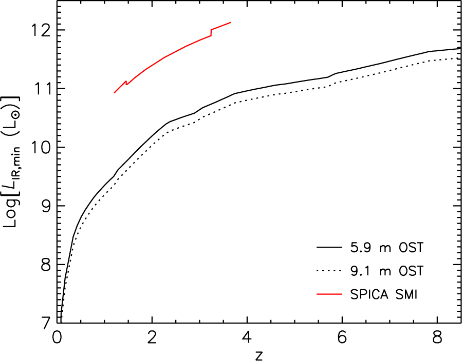
Figure 18. Comparison of the minimum L IR reachable with SPICA/SMI and OST/OSS, as a function of redshift. The upper solid (red) line shows the estimate by Kaneda et al. (Reference Kaneda2017, lower panel of their Figure 4) for galaxies with 100% SF detected via the 6.6, 7.7, 8.6, and 11.3 μm PAH features in their ‘deep survey’ (565.5 h of observing time, without overheads, over an area of 1 deg2). The lower solid (black) line and the dotted line show the corresponding minimum L IR for OST/OSS surveys with a 5.9 or a 9.1 m telescope, respectively, over the same area and in the same observing time. The difference between the SPICA/SMI and the OST/OSS limiting L IR is actually bigger than that shown in this figure because the OST/OSS estimate takes into account the decrease of PAH luminosities with decreasing gas metallicity, while the SPICA/SMI estimate does not.
Ground-based (sub-)mm telescopes, such as the Atacama Large (sub-)Millimeter Array (ALMA), the NOrthern Extended Millimeter Array (NOEMA), and the Large Millimeter Telescope (LMT), are allowing us to extend the detection of long-wavelength far-IR and sub-mm lines to higher redshifts. Further substantial progress is expected with new instruments, such as CCAT-prime (Stacey et al. Reference Stacey, Hailey-Dunsheath, Ferkinhoff, Nikola, Parshley, Benford, Staguhn and Fiolet2018) and the Atacama Large-Aperture Submm/mm Telescope (AtLAST; Bertoldi Reference Bertoldi2018).
8. Summary
The unprecedented sensitivity of the OST with the OSS instrument will allow us to address a variety of open issues concerning the evolution of galaxies and AGNs. To illustrate its potential, we estimated the counts of 53 IR spectral lines (9 of them are typical AGN lines). This was done by coupling relationships between line and IR continuum luminosity (or bolometric luminosity in the case of AGNs) with the SFR and luminosity functions by Cai et al. (Reference Cai2013), which accurately match the observational data. We have adopted the relationships found by Bonato et al. (Reference Bonato2014a,b, Reference Bonato2015, Reference Bonato2017b) for the SF contribution to the emission of 22 IR fine-structure lines and 6 PAH lines, and for the AGN emission of 27 IR lines. For the SF contribution of 3 lines, the relationships were recalibrated using new data, and new relationships were determined for 10 CO lines, for the SF contribution to 3 lines, and for the AGN contribution to 5 lines. We took into account the dependence of the starburst lines on gas metallicity.
We have compared the outcomes of blind surveys with two concepts for the OST, a 5.9 m telescope (Concept 2) and 9.1 m telescope (Concept 1). Our analysis found no compelling scientific case for the larger telescope.
We then investigated in more detail the performance of the 5.9 m telescope option for different surveyed areas, at fixed observing time. The number of line (and source) detections steadily increases with increasing area. Focussing on two extreme cases—surveys of 1 and 10 deg2, each with an observing time of 1 000 h—we find that both can detect emission lines associated with SF (allowing the estimate of the SFR) up to z≃8.5 (i.e. all the way through the reionisation epoch), and AGN lines (allowing an estimate of the bolometric luminosity) up to z≃5.5.
The larger area survey will detect ∼8.7×10⁶ lines from ∼2.7×10⁶ SFGs and ∼3.8×10⁴ lines from 3.5×10⁴ AGNs. It will generally provide better statistics, except at the highest redshifts where, however, the advantage of the deeper survey is modest and the statistics are poor anyway. The deeper survey will do significantly better only for some metallicity diagnostics at z > 4, and to investigate the poorly known dependence of the PAH emission (and, more generally, of L IR) on metallicity.
Both surveys will almost completely resolve the cosmic SFR density. OST with OSS will provide estimates of the IR luminosity function down to below the characteristic luminosity L ⋆ up to z ≃ 6. Thus it will allow us to reconstruct essentially the full SF history, complementing the information from ultra-deep surveys at near-IR wavelengths, which miss heavily dust-enshrouded galaxies. It will also allow us to learn about the evolution of metallicity and the physical conditions in the ISM up to very high redshifts. Note the key role played by the large OST/OSS field of view: we are dealing here with rare sources that cannot be picked up in statistically significant numbers by surveys with the James Webb Space Telescope, which can hardly be expected to carry out deep surveys over areas much larger than 100arcmin 2 (e.g. Finkelstein et al. Reference Finkelstein, Dunlop, Le Fevre and Wilkins2015).
The model also gave us the probability distributions that an object at redshift z has a starburst IR luminosity L IR,SF or an AGN bolometric luminosity L AGN, given the total luminosity L tot = L IR,SF + L AGN. Our approach to deriving the line luminosity functions allowed us to obtain, at the same time, luminosities of all the lines of both the SF and the AGN components of each simulated object. We could thus estimate for how many objects both components will be detectable, given the survey sensitivity and the number of objects that will be detectable in two or more lines.
This allowed us to investigate the OST/OSS potential to provide insight into galaxy-AGN co-evolution. We found that the OST will be able to probe BH mass growth by large factors, especially, but not only, at moderate redshifts (z ≲ 3) and for luminous sources (star-formation plus AGN luminosity ≳1013 L⊙). Spectroscopic surveys with OST will thus be a powerful tool to get a census of faint AGNs inside dusty SFGs over a broad redshift range.
Compared to SPICA/SMI, which is also expected to carry out blind surveys similar to those discussed here, the OST/OSS will reach, in the same amount of observing time, fluxes more than a factor of 10 fainter and will detect galaxies with L IR below 1012 L⊙ up to z≃8, while the SPICA/SMI is limited to z ≲ 4.
On the basis of the existing simulations (Bonaldi et al. Reference Bonaldi, Bonato, Galluzzi, Harrison, Massardi, Kay, De Zotti and Brown2019) and our estimates, we expect that the OST/OSS will be able to measure redshifts of a substantial fraction of the galaxies detected by the Square Kilometre Array (SKAFootnote j) deep surveys. The SKA will provide an independent estimate of the SFR in these galaxies and will also not be affected by obscuration (see Mancuso et al. Reference Mancuso2015, e.g. their Figure 12), but SKA measurements will be susceptible to contamination by nuclear radio activity. Together, OST and SKA will provide a more comprehensive view of the galaxy/AGN evolutionary scenario over a broad frequency range.
Acknowledgements
The authors thank Roberto Maiolino and Alessandro Bressan for enlightening suggestions, and the anonymous referee for useful comments that led to substantial improvements in this paper. This study acknowledges partial financial support by the Italian Ministero dell’Istruzione, Università e Ricerca through the grant ‘Progetti Premiali 2012 - iALMA’ (CUP C52I13000140001). The work is also supported in part by PRIN–INAF 2014 ‘Probing the AGN/galaxy co-evolution through ultra-deep and ultra-high resolution radio surveys’, by PRIN–INAF 2012 ‘Looking into the dust-obscured phase of galaxy formation through cosmic zoom lenses in the Herschel Astrophysical Large Area Survey’ and by ASI/INAF agreement n. 2014-024-R.1. M.B. and G.D.Z. acknowledge support from INAF under PRIN SKA/CTA FORECaST. Z.Y.C. is supported by the National Science Foundation of China (grant No. 11503024). M.N. acknowledges financial support from the European Union’s Horizon 2020 research and innovation programme under the Marie Skłodowska-Curie grant agreement No 707601.
Author ORCIDs
Bonato M. https://orcid.org/0000-0001-9139-2342.
Appendix A. Model versus data
As mentioned in Section 1, our reference model was validated against a broad variety of multifrequency data available until 2014. Many additional data have accumulated since then. We have therefore decided to check the model’s consistency with these more recent data. Figure A1 shows that the differential counts yielded by the model are in excellent agreement with data from SCUBA 2 and ALMA surveys. As illustrated by the figure, the model includes contributions from different populations (normal and star-bursting late-type galaxies, proto-spheroidal galaxies) and takes into account the effect of gravitational lensing. The contribution of radio sources to the counts is from Tucci et al. (Reference Tucci, Toffolatti, de Zotti and Martínez-González2011).
As mentioned in 7.3, recent estimates have yielded space densities of z3 pt∼>4 dusty SFGs well in excess of model predictions. To check how our model behaves in this respect, we have compared the predicted redshift distribution with the estimate by Ivison et al. (Reference Ivison2016), based on a much larger sample than those previously available. To this end, we simulated the selection criteria applied by Ivison et al. (Reference Ivison2016): S 500 μm ≥ 30 mJy and ultra-red colours in the Herschel/SPIRE bands (i.e. S 500 μm larger than both S 350 μm and S 250 μm). Moreover, we took into account the uncertainty in their photometric redshifts, Δz / (1+z) = 0.14. To the estimate of the total number of galaxies satisfying their selection criteria, Ivison et al. (Reference Ivison2016) applied a large correction for incompleteness (a factor of 36.0±8.2); the result is therefore quite uncertain. Thus, we have chosen to compare model predictions with the redshift distribution normalised to the number of objects. As illustrated by Figure A2, we find good agreement with the shape of the distribution, although the normalisation is low by a factor of ≃2.5.
Furthermore, the model, coupled with the well-established correlation between radio and far-IR emission, successfully reproduces the radio luminosity functions of SF galaxies, which is observationally determined up to z≃5 (Bonato et al. Reference Bonato2017a).
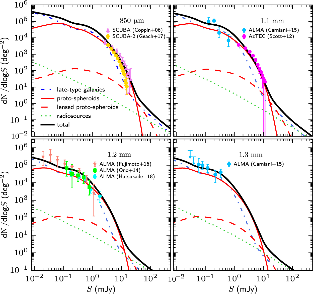
Figure A1. Comparison of the predictions of the Cai et al. (Reference Cai2013) model with differential counts from recent SCUBA 2 and ALMA surveys. The data are from Coppin et al. (Reference Coppin2006), Scott et al. (Reference Scott2012), Ono et al. (Reference Ono, Ouchi, Kurono and Momose2014), Carniani et al. (Reference Carniani2015), Fujimoto et al. (Reference Fujimoto, Ouchi, Ono, Shibuya, Ishigaki, Nagai and Momose2016), and Hatsukade et al. (Reference Hatsukade2018).
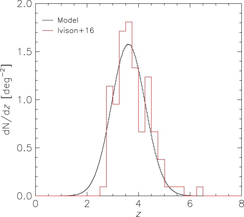
Figure A2. Comparison between the Ivison et al. (Reference Ivison2016) redshift distribution and the theoretical one derived from the Cai et al. (Reference Cai2013) model.