


Introduction
With the in-depth exploration of the microscopic world at the nanoscale, precision instruments capable of micro-nano imaging or manipulation, such as the atomic force microscope (AFM) (Fantner et al., Reference Fantner, Schitter, Kindt, Ivanov, Ivanova, Patel, Holten-Andersen, Adams, Thurner and Rangelow2006), the atomic force acoustic microscope (Yip et al., Reference Yip, Cui, Sun and Filleter2019), the microperforator (Sun et al., Reference Sun, Liu, Fan, Wang, Chen, Tian, Sun and Xie2020), and the nanopositioning stage (Fleming & Yong, Reference Fleming and Yong2017), have become indispensable in a lot of studies. As a representative, the AFM plays an important role in many fields due to its irreplaceable advantages (Schitter et al., Reference Schitter, Thurner and Hansma2008; Rana et al., Reference Rana, Pota and Petersen2014). For example, in the field of life science, the AFM can be used to observe the surface morphology of molecules (Dufrêne et al., Reference Dufrêne, Ando, Garcia, Alsteens, Martinez-Martin, Engel, Gerber and Müller2017), cells (Ren & Zou, Reference Ren and Zou2018), and biopolymers (Hartman & Andersson, Reference Hartman and Andersson2018), to image biological processes in real time (Fantner et al., Reference Fantner, Barbero, Gray and Belcher2010; Uchihashi et al., Reference Uchihashi, Watanabe, Fukuda, Shibata and Ando2016), to measure the mechanical properties of cells (Roduit et al., Reference Roduit, van der Goot, De Los Rios, Yersin, Steiner, Dietler, Catsicas, Lafont and Kasas2008; Schillers et al., Reference Schillers, Medalsy, Hu, Slade and Shaw2016), to characterize organelles and microorganisms inside cells (Janel et al., Reference Janel, Popoff, Barois, Werkmeister, Divoux, Perez and Lafont2019), to study the diseases such as atherosclerosis (Berquand et al., Reference Berquand, Wahart, Henry, Gorisse, Maurice, Blaise, Romier-Crouzet, Pietrement, Bennasroune, Sartelet, Jaisson, Gillery, Martiny, Touré, Duca and Molinari2021), etc. In the field of materials science, the AFM can be applied to study the size-dependent mechanical properties and photomechanical fatigue of diarylethene molecular crystals (Lansakara et al., Reference Lansakara, Tong, Bardeen and Tivanski2020), to measure adhesion energies between ultraflat graphene and a broad range of materials (Jiang & Zhu, Reference Jiang and Zhu2015), etc.
In many research works, it is important to use AFMs to image samples. Although AFMs have nanoscale imaging accuracy in theory, many error sources still degrade the imaging quality. Errors causing image distortion can be divided into four categories according to different sources, namely, the scanning system, the tip–surface interaction, the external environment, and data processing (Ricci & Braga, Reference Ricci and Braga2004; Marinello et al., Reference Marinello, Carmignato, Voltan, Savio and De Chiffre2010). The distortion induced by these errors is reflected as the image deformation in the horizontal direction and the artifacts of the topographic image in the vertical direction. Particularly, vertical drift and illusory slope are representative error sources to cause vertical artifacts in the obtained topography image, which make it difficult to truly represent the topography of the sample surface.
In reality, it is not easy to completely define the causes of vertical drift since it is excited by multiple error sources, e.g., environmental noise, external disturbance, temperature variation, etc. Image distortion induced by vertical drift is clearly represented as random vertical shifts of the morphology profiles in different fast scanning lines, thus producing the artificial ripples in the morphology image. Although improving the hardware performance and equipping more pure experimental environments, such as vibration damping platforms, isolation hoods, and ultra-clean room environment, e.g., can reduce the damage of vertical drift on the AFM imaging quality, many commercial AFMs are still suffering from drift-induced distortion due to uncontrollability and randomness of vertical drift. Therefore, commercial AFM systems usually perform line fitting row by row on the obtained topographic images to correct distortion (Starink & Jovin, Reference Starink and Jovin1996; Zahl et al., Reference Zahl, Bierkandt, Schröder and Klust2003; Hermanowicz et al., Reference Hermanowicz, Sarna, Burda and Gabryś2014; Jones et al., Reference Jones, Yang, Pennycook, Marshall, Van Aert, Browning, Castell and Nellist2015). In addition, many advanced correction algorithms have been developed to compensate for vertical drift online to achieve high-quality imaging, including designing a robust controller (Yi et al., Reference Yi, Li and Zou2018), improving scanning algorithms (Lapshin, Reference Lapshin2007; Marinello et al., Reference Marinello, Bariani, De Chiffre and Savio2007; Li et al., Reference Li, Wang and Liu2012), and upgrading imaging algorithms (Clifford & Seah, Reference Clifford and Seah2009; Erickson et al., Reference Erickson, Coquoz, Adams, Burns and Fantner2012; Wu et al., Reference Wu, Fang, Fan, Wang and Liu2020).
The illusory slope refers to the slant angle between the horizontal scanning plane of the AFM and sample surface, which causes an artificial tilt in the constructed topography image. The illusory slope is mainly induced by such factors as installation slope (Marinello et al., Reference Marinello, Carmignato, Voltan, Savio and De Chiffre2010), cantilever-sample tilt angle (D'Amato et al., Reference D'Amato, Marcus, Eriksson and Carpick2004), and creep of the scanner in the vertical direction (Han & Chung, Reference Han and Chung2011). To correct the slope-induced image distortion, various leveling algorithms have been proposed to subtract the slope from the topography image, wherein the key is to accurately fit the inclined plane. For instance, Han & Chung (Reference Han and Chung2011) proposed a new method to obtain the tilt angle by using only two scanned images with no special tools. Dong et al. (Reference Dong, Fang, Zhang and Ren2014) designed a real-time preprocessing approach based on the recurrent least square method for slope elimination. Wang et al. (Reference Wang, Lu, Li and Wang2018) proposed a two-step scheme based on image segmentation to achieve optimized image flattening in an automated manner. Yang et al. (Reference Yang, Wang, Hao, Yang, Shi and Yu2020) proposed an adaptive algorithm to remove the detorsion background based on the improved image edge detection method.
Inspired by the above research work, this paper proposes an advanced correction algorithm based on sparse sample consensus (SPASAC), which realizes the synchronous correction of the image distortion caused by vertical drift and slope. Specifically, since abnormal points and some local height data likely impair the validity of line fitting, this paper first utilizes the laser spot voltage error during the scanning process to develop an adaptive filtering algorithm, so as to achieve the preprocessing of the topography height and acquire the candidate data for further line fitting. In addition, considering that the fluctuation of the cross-sectional profile still damages the accuracy of line fitting, this paper designs a robust line fitting algorithm based on SPASAC, which can automatically generate the optimal fitting result to match the datum line of each profile curve, based on which the image distortion is corrected by subtracting the fitted lines from the distorted image. Finally, convincing experiments are provided to verify the satisfactory performance of the proposed algorithm in correcting AFM image distortion.
The contributions of the paper lie in the following aspects: (1) a novel data preprocessing algorithm is designed to achieve effective filtering for height data obtained by AFM scanning; (2) an adaptive SPASAC-based method is proposed to improve the accuracy and robustness of line fitting for the morphology profile; (3) the proposed method has the ability to simultaneously correct the drift-induced distortion and the slope-caused distortion, in addition, the method does not require any hardware improvements or online algorithm modifications, which thus has strong applicability and portability.
The reminder of the paper is organized as follows: the AFM Image Distortion Analysis section illustrates the image distortion in detail. The Image Distortion Correction section discusses the difficulties in image correction, elaborates the basic idea of the proposed algorithm, implements preprocessing for the height data, and designs the adaptive line fitting algorithm, thus achieving the image distortion correction. The Experiments and Applications section demonstrates the correction performance of the proposed algorithm. Finally, the Conclusions section summarizes the paper and prospects the future research work.
AFM Image Distortion Analysis
To intuitively present the distortion caused by vertical drift and slope, the imaging results of an optical grating sample are provided in Figure 1. Specifically, the optical grating sample has fixed periodic bulges on the flat substrate, the standard topographic image without distortion is shown in Figure 1a1 with the three-dimensional image presented in Figure 1a2, which exhibits that the sample features are smooth and level.

Fig. 1. The standard topographic image and distorted topographic images of a calibrated grating sample.
Vertical Drift
The distorted image due to vertical drift is presented in Figure 1b1 with the three-dimensional topographic image shown in Figure 1b2, which contains multiple irregular striped artifacts along the  $x$-direction (fast scanning direction). Since the fast scanning process of each line is very short, the height drift of different scanning points on each line is regarded as the same, and uncontrollable offsets of the profiles on different lines are random, thus generating ripples in the topographic image. To correct the image distortion, a widely used method in commercial AFMs is to perform line fitting for each line to calculate the offset, so as to eliminate the artifacts of the morphology image.
Illusory Slope
Besides, Figure 1c1 exhibits the image distortion due to illusory slope, it can be seen that the features on the left are obviously brighter than those on the right, which reflect that the morphology on the left is higher than that on the right. Accordingly, the three-dimensional topographic image in Figure 1c2 clearly shows the tilt angle between the  $x$–
$x$– $y$ plane and the sample surface caused by an illusory slope. Due to the consistency of the tilt, a common method is to implement surface fitting to remove the artificial slope in the image and make the reference plane of the sample topography parallel to the horizontal plane.
Coupling of Vertical Drift and Slope
In addition, vertical drift and illusory slope are coupled together to generate distorted images in Figures 1d1 and 1d2, which contain the mixed artifacts of ripples and tilt. Through the above analysis, it may be feasible to correct the profile height of each line to eliminate the distortion caused by vertical drift and slope at the same time. Therefore, it is worthwhile to make efforts to design a line fitting-based image correction algorithm with generality and robustness, thus constructing high-quality sample topography images.
Image Distortion Correction
Basis Idea of the Proposed Method
For many samples, especially for such samples as cells, the cross-sectional profile is often obviously undulating, which greatly increases the difficulty of line fitting. Meanwhile, the features of the sample appeared as bulge or concave further inevitably damage the accuracy of line fitting. Figure 2 shows the illustration of line fitting and correction of the cross-sectional profile. Specifically, the solid curve in Figure 2a presents a distorted cross-sectional profile of a cell sample obtained by AFM scanning with vertical drift and slope, where the raised area marked by circles represents the feature of the sample. When line fitting is directly performed for the profile curve, the obtained optimal straight line is shown as the dot-dashed line in Figure 2a, which obviously deviates from the desired line shown as the dashed line. Subsequently, the fitted line and the desired line are subtracted from the profile curve, respectively, and the corrected profile curves are shown in Figure 2. The dot-dashed curve corresponds to the corrected profile based on line fitting, which is still distorted compared with the desired correction result shown as the dashed curve.

Fig. 2. The illustration of line fitting and correction of the profile.
The reason for this problem is that the feature area in the sample interferes with line fitting, which makes it difficult to accurately model the vertical drift and slope. Therefore, the key to image correction is to adaptively eliminate the interference of outliers, e.g. sample feature area and other abnormal data, so as to extract the effective data in the profile to achieve accurate line fitting. To address this issue, the paper designs a robust line fitting algorithm, which includes two steps of data preprocessing and line fitting. Specifically, the preprocessing is to adopt the laser spot error of AFM scanning to coarsely filtrate the profile height, thereby improving the efficiency of the algorithm. Line fitting is implemented based on an SPASAC algorithm. Through continuous iteration, the fitted line is able to free from the disturbance of outliers to accurately simulate vertical drift and slope, based on which the distorted image is corrected to truly reflect the topography height of the sample. The flow chart of the proposed image correction algorithm is shown in Figure 3.

Fig. 3. Flow chart of the proposed image correction algorithm.
Preprocessing Based on Laser Spot Error
For the profile of a line with  $N$ scanning points, the topography height of the $n$th point is calculated as follows:
 $$h_{n} = k_{{\rm tc}}[ u_{n}-( V_{{\rm sp}}-e_{n}) /k_{{\rm sc}}] ,\; \quad n\in{ 1,\; 2,\; 3,\; \ldots,\; N} ,\; $$
where  $u_{n}$ represents input voltage for the piezoelectric scanner in the $z$-direction, $V_{{\rm sp}}$ denotes the given reference voltage, $e_{n}$ is referred as the laser spot error in this paper, which denotes the difference between the given reference voltage $V_{{\rm sp}}$ and the voltage of the reflected laser beam detected by the laser detector in the $z$-direction. $k_{{\rm tc}}$ denotes the telescopic coefficient of the scanner, and $k_{{\rm sc}}$ is the sensitivity coefficient of the system.
For each scanning point, there is a certain correlation between the laser spot error and the topography height. As shown in Figure 4, the laser spot error, corresponding to the scanning points in the feature area, has more obvious fluctuations. Therefore, it is feasible to utilize the laser spot error to roughly filter the height data of the profile to eliminate some outliers.

Fig. 4. The illustration of the correlation between the laser spot error and the topography height.
Specifically, for a fast scanning line, the absolute value of the difference of the laser spot error is first calculated as follows:
 $$\vert \Delta e_n\vert = \left\{\matrix{ \vert e_{n + 1}-e_n\vert ,\; \hfill & n\in{ 1,\; 2,\; 3,\; \ldots,\; N-1} \hfill \cr 0,\; \hfill & n = N \hfill }\right..$$
 Afterward, the alternative scanning points in the profile, used for line fitting in the next step, are defined as  $( x_m,\; h_m)$, where the index $m$ satisfies the following constraints:
 $$\vert \Delta e_m\vert < \vert \Delta e_{n_o}\vert ,\; \quad m\in{\opf M}^{1\times M} \subset { 1,\; 2,\; 3,\; \ldots,\; N} ,\; $$
where  $\vert \Delta e_{n_o}\vert$ represents the best threshold that can distinguish the substrate and the feature area in the profile. In detail, $\vert \Delta e_1\vert ,\; \vert \Delta e_2\vert ,\; \vert \Delta e_3\vert ,\; \ldots ,\; \vert \Delta e_N\vert$ are classified into two categories, and the best threshold $\vert \Delta e_{n_o}\vert$ is determined when the variance between the two categories is the largest. Therefore, the index $n_o$ is determined as follows:
 $$n_o = \arg\max \mu_{n_o}\mu_{N-n_o}\vert \delta_{n_o}-\delta_{N-n_o}\vert ,\; $$
where  $n_o\in { 1,\; 2,\; 3,\; \ldots ,\; N-1}$, $\mu _{n_o}$ and $\mu _{N-n_o}$ denote the probability of each category, $\delta _{n_o}$ and $\delta _{N-n_o}$ stand for the mean level of each category, which are calculated as follows:
 $$\mu_{n_o} = \sum^{n_o}_{n = 1}\vert \Delta e_n\vert ,\; \quad \mu_{N-n_o} = \sum^{N}_{n = n_o + 1}\vert \Delta e_n\vert ,\; $$
 $$\delta_{n_o} = \sum^{n_o}_{n = 1} {n\vert \Delta e_n\vert \over \mu_{n_o}},\; \quad \delta_{N-n_o} = \sum^{N}_{n = n_o + 1} {n\vert \Delta e_n\vert \over \mu_{N-n_o}}.$$
Line Fitting Based on SPASAC
As a widely used method, the random sample consensus (RANSAC) algorithm is able to estimate the parameters of the mathematical model from a set of observed data containing correct data (inliers) and abnormal data (outliers). However, this algorithm needs the probability of the interiors in advance. In addition, the algorithm is nondeterministic due to the random sampling, which implies that the modeling result is reasonable under a certain probability and the probability increases with more iterations. Therefore, there is no guarantee that the algorithm can produce the optimal result.
Hence, inspired by the RANSAC algorithm, an SPASAC-based line fitting algorithm is proposed in this section, which can obtain the best fitting result under the premise of unknown interiors probability. The proposed method adopts a traversal method to sparsely sample two scanning points in sequence to perform line fitting and evaluates the model by calculating the error rate between the heights of the scanning points and the fitted line. The model with the lowest error rate is determined as the optimal fitting result.
More specifically, for the alternative point  $( x_m,\; h_m)$, $m\in {\opf M}^{1\times M}$, when selecting two different points in turn to construct a line, a total of ${M( M-1) }/{2}$ straight lines can be obtained, which are denoted as follows:
 $$l_p\, \colon \, a_px + b_ph + c_p = 0,\; \quad p\in\left\{1,\; 2,\; 3,\; \ldots,\; {M( M-1) \over 2}\right\},\; $$
where  $a_p$, $b_p$, and $c_p$ represent the parameters of the $p$th straight line, which are determined by the alternative points.
Afterward, the distance from each point  $( x_m,\; h_m)$ to the straight line $l_p$ is calculated as follows:
 $$d_{\,pm} = {\vert a_px_m + b_ph_m + c_p\vert \over \sqrt{a_p^{2} + b_p^{2}}}.$$
For each straight line, the smaller the distance  $d_{pm}$, the greater the probability that the point $( x_m,\; h_m)$ is on the line $l_p$. Therefore, it implies that the fitted line is more likely to be the optimal result when more points are on or near the line.
Furthermore, the distance  $d_{pm}$ is compared with the given threshold $\alpha$, and the number of points whose distance is less than $\alpha$ is counted and recorded as $N_p$, which is determined as follows:
 $$N_p = \left\{\matrix{ N_p + 1,\; \hfill & d_{\,pm}< \alpha\hfill \cr N_p,\; \hfill & d_{\,pm}\geq\alpha \hfill }\right.,\; $$
where  $N_p$ is initialized to 0.
Hence, for all the obtained straight lines, the line with the maximum value of  $N_p$ is the optimal result, which is denoted as follows:
 $$l_{\,p_o}\, \colon \, \ a_{\,p_o}x + b_{\,p_o}h + c_{\,p_o} = 0,\; \quad b_{\,p_o}\neq 0,\; $$
where
 $$p_o = \mathop{\arg\max} N_{\,p_o},\; \quad p_o\in\left\{1,\; 2,\; 3,\; \ldots,\; {M( M-1) \over 2}\right\}.$$
 For the scanning point  $( x_n,\; h_n)$ on the profile, the projection of the point on the line $l_{p_o}$ along the vertical direction is calculated as $\tilde {h}_n = -{( a_{p_o}x_n + c_{p_o}) }/{b_{p_o}}$. Therefore, the distorted profile is corrected by subtracting $\tilde {h}_n$ from the scanned height $h_n$ as follows:
 $$\hat{h}_n = h_n-\tilde{h}_n = h_n + {a_{\,p_o}x_n + c_{\,p_o}\over b_{\,p_o}}.$$
According to the above method, preprocessing and line fitting are performed for each profile of the scanning line in the distorted image, and the image is adaptively corrected to eliminate distortion induced by vertical drift and illusory slope.
Experiments and Applications
In the experiments and applications, a commercial Nanosurf Flex-FPM AFM system is adopted to generate morphology images of samples. The scanning process is carried out with the contact mode in air, and the scanning frequency is set to 1 Hz. After obtaining the distorted image, the proposed method is implemented to correct the image. Meanwhile, to fully demonstrate the performance of the proposed algorithm, the commercial line fitting algorithm is also adopted to correct the image for comparison. The commercial algorithm performs line fitting for the measured height profile of each fast scanning line by using the least-quares method, and the final morphological height of each line is produced by subtracting the fitted straight line from the measured height profile, so as to correct the image distortion.
Experiment of an Optical Grating Sample
In the experiments, a calibrated optical grating sample is selected to perform imaging and correction. The sample has an approximate feature height of  $20\, {\rm {nm}}$ with a fixed period of about $3\, {\rm {\mu m}}$, where the raised part and the base part are both horizontal and flat. The imaging size is set to $6\, \mu {\rm m}\times 6\, \mu {\rm m}$, the obtained distorted topography image is presented in Figure 5a1, and the corresponding three-dimensional topography image is shown in Figure 5a2. Due to vertical drift and slope, the image is obviously tilted, the feature area and the base part are no longer flat, which makes it difficult to reflect the true topographic features of the sample.

Fig. 5. The distorted topographic image and corrected topographic images of an optical grating sample.
Afterward, the distorted image is corrected by the commercial method with the correction results presented in Figures 5b1 and 5b2. It can be seen that, compared with the distorted image obtained by AFM scanning, the morphology image becomes clear and level, the raised feature area becomes more prominent, which implies that the illusory slope is effectively corrected. However, due to the limitation of line fitting in the commercial method, for the line profile that does not contain the feature area, it is significantly higher than the substrate in the profile containing the feature area, which results in the formation of artificial rectangular grooves in the topographic image. The results indicate that the commercial algorithm does not completely correct image distortion caused by vertical drift although it partly improves the imaging quality of the AFM.
Subsequently, the proposed method is implemented to correct the distorted image with the correction result shown in Figure 5c1 and the corresponding three-dimensional image presented in Figure 5c2. It can be seen from the correction results that the base part of the topography image is uniformly level and flat, and the topography of the raised feature area is regular and clear, which can truly reflect the surface topography of the grating sample, thus verifying the good performance of the proposed method.
Moreover, to further intuitively compare the correction performance, the cross-sectional profiles of the same line along the  $x$-direction in the distorted image and the corrected images are plotted in Figure 6. Specifically, the profile of the distorted image in Figure 5a1 is plotted as the solid curve, which has an illusory slope with the tilt angle of about $6^{\circ }$. In the profile, the raised parts denote the sample feature while the lower areas correspond to the substrate of the sample. Ideally, the line fitting result should coincide with the substrate, so as to accurately eliminate the artifact induced by vertical drift and slope. However, limited by the applicability, the fitted line of the commercial method with the tilt of about $3^{\circ }$, shown as the solid line with plus sign, obviously deviates from the substrate, which leads to the issue that the correction result, shown as the dotted curve, still has an artificial tilt and the profile height is also distorted. Otherwise, for the proposed method, since the fitted line, presented as the dashed line, can approximate the profile of the sample substrate, the feature area and the base part in the correction result are basically level as the dot-dashed curve, which are more consistent with the true sample morphology.

Fig. 6. Cross-sectional profiles along the  $x$-direction in the morphology images of the optical grating sample.
Although the slope correction performance is effectively verified by comparing the profiles in the  $x$-direction, the correction effect of drift-caused distortion is not demonstrated since it is induced by the offsets of the profiles between different fast scanning lines in the $x$-direction. Therefore, the same cross-sectional profiles along the $y$-direction in Figures 5a1, 5b1, 5c1 are selected to further verify the drift correction effect. As shown in Figure 7, the solid curve denotes the distorted profile, which cannot present the morphology feature due to the damage of vertical drift. Afterward, the correction results of the commercial method and the proposed one are plotted as the dotted curve and the dot-dashed curve, respectively. It can be seen that the height of the feature area in the corrected profile of the commercial method is lower than the actual height of $20\, \rm {nm}$, while the correction result of the proposed method is closer to the actual morphology of the sample, thus indicating the satisfactory effect of the proposed algorithm.

Fig. 7. Cross-sectional profiles along the  $y$-direction in the morphology images of the optical grating sample.
Application on a Biological Cell Sample
Furthermore, the sample of Escherichia coli is scanned to verify the applicability of the proposed method. As a smooth colony, E. coli cells are typically rod-shaped with the length of 1.0–3.0  $\mu$m and the diameter of 0.25–1.0 $\mu$m. The sample is made by culturing E. coli cells on the flat polydimethylsiloxane surface. The bacteria is immobilized on the gelatin-coated mica surface, and the imaging process is carried out by the AFM with the contact mode in air. Specifically, a small quantity of the bacteria is scraped off of a culture plate and transferred into a micro-centrifuge tube containing distilled water, then, the mixed aliquot is pipetted onto a gelatin treated mica disk and spread with the pipette tip to a diameter of about $1\, {\rm cm}$, and the E. coli sample is finally blow-dried for imaging in air. Therefore, in the absence of image distortion, the sample substrate in the topography image should be relatively flat while the topography of the cell area is smoothly convex.
The experimental results are presented in Figure 8. Specifically, the topography image obtained by AFM scanning is shown in Figure 8a1. It can be seen that there are obvious artificial ripples on the surface of the sample induced by vertical drift. Moreover, the left area of the image is closer to red while the right area is closer to blue, which means that the left area is significantly higher than the right area due to the vertical slope. Meanwhile, Figure 8a2 exhibits the three-dimensional topographic image corresponding to Figure 8a1, which more intuitively presents the artificial fluctuation of the sample surface and the tilt angle between the sample surface and the horizontal plane.
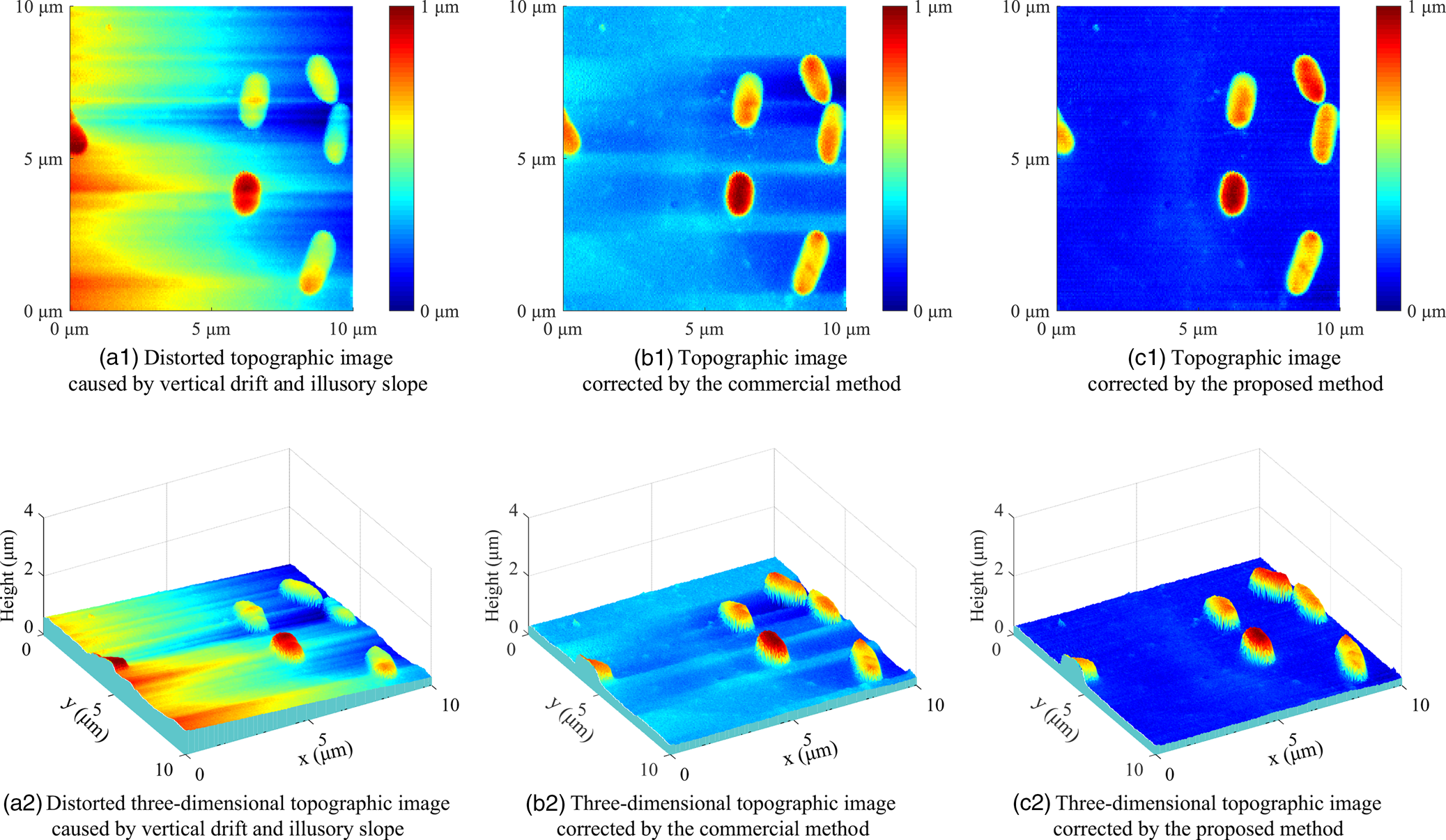
Fig. 8. The distorted topographic image and corrected topographic images of an E. coli sample.
Furthermore, the distorted image is processed by the commercial line fitting algorithm with the correction result presented in Figure 8a2. Compared with the distorted image, the color distribution in the corrected image is more uniform, and the color of the left area is close to that of the right area, indicating that the sample surface is relatively horizontal, which demonstrates that the slope of the topographic image has been eliminated. Besides, the ripples in the topography image are also significantly reduced compared with the distorted image, especially, the ripples are completely eliminated for the rows without cells. However, there are still obvious ripples on the rows of the image where the cells are located. The reason for this issue is that the precision of the direct line fitting in the commercial algorithm is impaired by the height of the cell morphology, the fitting result is thus difficult to accurately simulate thermal drift and slope, which results in a slight distortion of the correction result. Meanwhile, the corresponding three-dimensional image in Figure 8b2 also clearly demonstrates that the slope has been basically corrected while there are still some artificial ripples in the topographic image.
Afterward, the proposed method is performed to correct the distorted image, the corrected topographic image is shown in Figure 8c1 with the corresponding three-dimensional image presented in Figure 8c2. It can be seen that the color of the substrate in the image is basically the same, which demonstrates that the sample surface is flat and level. Moreover, the color of the corrected cell area is also more uniform, indicating that the height change of the cell topography is smoother. In addition, the three-dimensional topography image more clearly presents the sample topography with high quality, which verifies that the proposed method is able to correct the image distortion caused by vertical drift and slope.
To quantitatively verify the image quality, two common image evaluation indexes, namely root-mean squared error (RMSE) and peak signal to noise ratio (PSNR), are calculated for the distorted image, the corrected images of the commercial method, and the proposed method. The calculation results of RMSE and PSNR are presented in Table 1. For the topography image, the smaller the value of RMSE, the smaller the topography fluctuation. Hence, the RMSE value of the image after correction is smaller than that of the distorted image ( $0.47\, \mu {\rm m}$), and the RMSE of the proposed method ( $0.23\, \mu {\rm m}$) is less than $0.32\, \mu {\rm m}$ of the commercial method, which indicates the better performance of the proposed method. Otherwise, as an objective standard for evaluating images, a larger PSNR means less image distortion. As shown in Table 1, the PSNR is 6.48 dB for the distorted image, 9.86 dB for the image corrected by the commercial method, and 12.72 dB for the corrected image of the proposed method, which verifies that the proposed method can correct image distortion more effectively.
Table 1. RMSE and PSNR of the Distorted Image, the Corrected Images of the Commercial Method, and the Proposed Method

Subsequently, the cross-sectional profiles of the same line along the  $x$-direction in different images are provided in Figure 9 to further demonstrate the performance of slope elimination. In detail, the solid curve denotes the distorted profile of Figure 8a1 obtained by AFM scanning, which presents a clear slope with the tilt angle of about $16^{\circ }$. The two raised areas in the profile represent the cell morphology. The solid line with plus sign stands for the fitted line of the commercial method, which has a tilt of $10^{\circ }$ on the $x$-axis and is significantly deviated from the distorted profile. This is because the cell areas on the right side of the distorted profile are relatively high, which affects the line fitting of the commercial algorithm, thus resulting in the deviation between the fitted line and the substrate of the distorted profile. Otherwise, the dashed line presents the fitted line of the proposed method with a tilt of $15.9^{\circ }$ on the $x$-axis, which is close to the distorted profile due to the robustness. Based on the line fitting results, the distorted profile is corrected with the results shown as the dotted curve for the commercial method and the dot-dashed curve for the proposed method. It can be seen that the corrected profile by the proposed method is substantially level while the profile of the commercial method still tilts with about $6^{\circ }$ on the $x$-axis.

Fig. 9. Cross-sectional profiles along the  $x$-direction in the morphology images of the E. coli sample.
Similarly, the cross-sectional profiles of the same line along the  $y$-direction in the distorted image and the corrected image are plotted in Figure 10 to further compare the performance of the vertical drift correction. The selected profile does not contain the cell area; therefore, the profile should be relatively flat theoretically. Meanwhile, the cross-sectional profile in the $y$-direction is level since the slope of the topographic image is along the $x$-direction. However, due to the vertical drift, the profile obtained by AFM scanning, shown as the solid curve, is distorted with pronounced fluctuations. Besides, the correction result of the commercial method is presented as the dotted curve, which is also distorted due to the limited applicability. Moreover, the corrected profile of the proposed method, plotted as the dot-dashed curve, is comparatively flat and level, which is closer to the true morphology of the substrate of the sample.

Fig. 10. Cross-sectional profiles of the substrate along the  $y$-direction in the morphology images of the E. coli sample.
As verified by the application for the E. coli cells, the proposed method works well when the differences in height are important and appear suddenly. Furthermore, for other biological samples, the applicability of the proposed method mainly depends on the size of the feature area of the sample. That is, for a biological sample, when the size of the sample feature occupies more than half of the specified imaging range in the fast scanning axis, the proposed method may not perform well. On the contrary, the proposed method can accurately correct image distortion for the sample with a small feature area, even if the differences of the sample height are small and appear gradually.
Conclusions
This paper proposes an effective correction algorithm for image distortion caused by vertical drift and slope. The algorithm has strong robustness since it includes two steps of data preprocessing and adaptive line fitting. Specifically, the laser spot voltage error signal is first used to filter the sample topography height data. On this basis, a line fitting algorithm based on SPASAC is designed to obtain the best fitting result for the profile of each fast scanning line, based on which the distorted surface of the entire image is obtained and the morphology image is accordingly corrected by eliminating the distortion. In the experiments and applications, by correcting the imaging results of a grating sample and an E. coli sample, it is verified that the proposed algorithm is able to achieve high-quality AFM imaging. Future work will focus on extending the practical application of the proposed algorithm in biology and other fields.
Acknowledgments
This work is supported by the National Natural Science Foundation of China under grant 62003172, grant 61633012, and grant 21933006. The authors would like to thank Professor Xizeng Feng from College of Life Sciences of Nankai University for providing Escherichia coli cells in this work.


