


1. Introduction
Hydrogen produced by water electrolysis using gas-evolving electrodes from renewable electricity is essential for achieving carbon neutrality and a sustainable future (Brauns & Turek Reference Brauns and Turek2020; Yue et al. Reference Yue, Lambert, Pahon, Roche, Jemei and Hissel2021; Shih et al. Reference Shih2022). However, micro- and nanobubbles formed at an electrode can result in undesired blockage of the electrode and thus decrease the energy transformation efficiency (Vogt & Balzer Reference Vogt and Balzer2005; Zhao, Ren & Luo Reference Zhao, Ren and Luo2019; Angulo et al. Reference Angulo, van der Linde, Gardeniers, Modestino and Rivas2020). Addressing this problem requires a deeper understanding of the dynamics of individual nanobubbles on electrodes. Recent advancements in experimental techniques have enabled the generation of single electrolytic nanobubbles (Luo & White Reference Luo and White2013; Liu et al. Reference Liu, Edwards, German, Chen and White2017; Edwards, White & Ren Reference Edwards, White and Ren2019). Though the formed single nanobubbles cannot be observed directly, their presence and equilibrium states are indicated by a sudden drop of the peak current to a steady value (Luo & White Reference Luo and White2013; Liu et al. Reference Liu, Edwards, German, Chen and White2017; Edwards et al. Reference Edwards, White and Ren2019). Numerical methods such as finite element or difference methods (Luo & White Reference Luo and White2013; Higuera Reference Higuera2021) and molecular dynamics simulations (Perez Sirkin et al. Reference Perez Sirkin, Gadea, Scherlis and Molinero2019; Maheshwari et al. Reference Maheshwari, Van Kruijsdijk, Sanyal and Harvey2020; Ma et al. Reference Ma, Guo, Chen and Zhang2021) have also been used to study the nucleation and stability mechanism of electrolytic nanobubbles. However, a fundamental theory for the statics and dynamics of single electrolytic nanobubbles is still lacking.
Electrolytic nanobubbles belong to the family of surface nanobubbles. Since their discovery in the 1990s, surface nanobubbles have triggered the fascination of scientists (Lohse & Zhang Reference Lohse and Zhang2015b) due to their unique properties such as their long lifetime (Lou et al. Reference Lou, Ouyang, Zhang, Li, Hu, Li and Yang2000; Weijs & Lohse Reference Weijs and Lohse2013) and their small contact angles (Zhang, Maeda & Craig Reference Zhang, Maeda and Craig2006), and because of their practical relevance and applications in flotation (Calgaroto, Wilberg & Rubio Reference Calgaroto, Wilberg and Rubio2014), nanomaterial engineering (Hui et al. Reference Hui, Li, He, Hu and Fang2009) and diagnostics (Batchelor et al. Reference Batchelor, Abou-Saleh, Coletta, McLaughlan, Peyman and Evans2020). Significant progress has been made (see the reviews Lohse & Zhang Reference Lohse and Zhang2015b; Tan, An & Ohl Reference Tan, An and Ohl2021) in developing new methods for generating and detecting nanobubbles, as well as clarifying their stability mechanism by an analytical model developed by Lohse & Zhang (Reference Lohse and Zhang2015a) (and extensions thereof), which suggests that a stable balance between the Laplace pressure-driven gas outflux and the local oversaturation-driven gas influx is made possible by contact line pinning.
This work aims to understand the dynamics of single electrolytic nanobubbles through molecular dynamics simulations and analytical theories. The Lohse–Zhang model is generalized to account for the gas produced at the contact line. The new model can quantitatively explain the conducted molecular simulations without any free parameters. This generalization thus creates a unified theoretical framework that can predict not only the equilibrium states of stable electrolytic nanobubbles (such as contact angles and the time required to reach equilibrium), but also the unbounded growth of unstable electrolytic nanobubbles, which eventually detach.
2. Molecular simulations
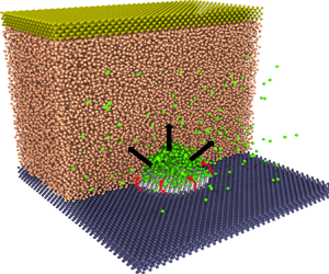
Molecular dynamics (MD) simulations are used as virtual experiments to simulate the generation of electrolytic nanobubbles on nanoelectrodes. We adopt the open-source code LAMMPS (Plimpton Reference Plimpton1995). As shown in figure 1(a), the minimal molecular system consists of water molecules (represented in orange), gas atoms (in green), atoms of the electrode (in white), atoms of the solid base (in blue) and atoms of the ‘piston’ plate (in bronze). The water is modelled by the monoatomic water (mW) potential (Molinero & Moore Reference Molinero and Moore2009), implying a surface tension  $\gamma =66\,{\rm mN}\,{\rm m}^{-1}$. Except for water itself, the intermolecular potentials $U$ between $i$-type atoms and $j$-type atoms are simulated with the standard Lennard-Jones (LJ) 12-6 potential:
 \begin{equation} U({{r}_{ij}}) = \begin{cases} 4\varepsilon_{ij} \biggl[ {{\left(\dfrac{\sigma_{ij} }{{{r}_{ij}}} \right)}^{12}}-{{\left(\dfrac{\sigma_{ij} }{{{r}_{ij}}} \right)}^{6}} \biggr] &\text{if } {{r}_{ij}}\le {{r}_{c}},\\ 0 & \text{if} {{r}_{ij}}>{{r}_{c}}, \end{cases} \end{equation}
where  $r_{ij},\varepsilon _{ij},\sigma _{ij}$ and ${r}_{c}$ are the pairwise distance, energy parameter, length parameter and cutoff distance, respectively. The cutoff distance is chosen as $r_c=16.5\,\unicode{x00C5}$. The complete list of parameters among the water (W), gas (G), electrodes (E), base solids (S) and piston (P) are given in table 1.

Figure 1. (a) A snapshot of the generated electrolytic nanobubble on the nanoelectrode in MD simulations. The simulated domain has been sliced to observe the bubble. The system's condition is maintained at temperature  $T=300$ K, pressure $P_{\infty }=10$ atm and gas concentration $C_{\infty }=c_s$ ( $c_s$ is the gas solubility). The nanoelectrode has a diameter $L=5.76$ nm and is made hydrophobic to water, while the surrounding solid is hydrophilic. Here $J_{in}$ represents the gas influx to the bubble produced at the contact line, while $J_{out}$ represents the diffusive outflux through the bubble interface. (b) Sketch of a growing bubble with pinning length $L$, contact angle $\theta (t)$, radius of curvature $R(t)$ and height $H(t)$.
Table 1. Interaction parameters.

Note that the atoms of electrodes and base solids are fixed so that there is no need to specify the interactions among them. The atoms of the piston move in the same phase so that the interactions inside them are also ignored.
The gas modelled by the standard LJ 12-6 potential has a density  $\rho _{\infty }=11.47\,{\rm kg}\,{\rm m}^{-3}$ at 10 atm and 300 K. The molar mass of the gas is $28\,{\rm g}\,{\rm mol}^{-1}$. The gas–water interaction is tuned to obtain a gas solubility $c_s=0.54\,{\rm kg}\,{\rm m}^{-3}$ (calculated using Henry's law) and a mass diffusivity $D=4.1\times 10^{-9}\,{\rm m}^{2}\,{\rm s}^{-1}$ (calculated using Einstein relation (Skoulidas & Sholl Reference Skoulidas and Sholl2005)). The electrochemical reaction that transforms water molecules into gas atoms is modelled in a simple way similar to previous MD studies (Perez Sirkin et al. Reference Perez Sirkin, Gadea, Scherlis and Molinero2019; Maheshwari et al. Reference Maheshwari, Van Kruijsdijk, Sanyal and Harvey2020; Ma et al. Reference Ma, Guo, Chen and Zhang2021) where right above the electrodes, two layers of water molecules can turn into gas atoms conducted at a fixed rate, leading to a constant gas influx $J_{in}$, i.e. a constant current $i_{in}$ (assuming the production of each gas atom needs a specific number of electrons). Note that the contact line of the bubble is fluctuating so that there are still some water molecules available on the electrode after bubble formation to ensure a constant $J_{in}$, which is the case for the simulations done in this work. However, for sufficiently large $J_{in}$, there can be a shortage of water molecules to keep a constant $J_{in}$.
By adjusting the water–electrode interaction  $\varepsilon _{we}$, the electrode is made hydrophobic with a water contact angle of $120^{\circ }$. Conversely, the base solid is set to be hydrophilic to water with a contact angle of $5^{\circ }$. Such settings force the bubble to be pinned around the electrode.
The box has a fixed lateral size ( $L_x=17.28$ nm, $L_y=17.28$ nm). The height of this box is adjusted to maintain the far-field pressure $P_{\infty }=10$ atm where periodic boundary conditions are applied in the other two directions. The initial thickness of the water slab is $11.3$ nm with 124 416 atoms. The thickness of the solid base is $0.96$ nm and has a face-centred cubic (fcc) structure with a number density $0.0332\,\unicode{x00C5} ^{-3}$. The far-field gas concentration is maintained at the gas solubility by switching the identity of gas atoms back into the identity of water atoms, performed in a box right below the piston. This process is carried out only when the gas concentration in the box is larger than the gas solubility.
As sketched in figure 1(a,b), after nucleation the bubble grows until the balance between the Laplace pressure-driven diffusive outfluxes ( $J_{out}$) and the reaction-driven gas influxes ( $J_{in}$) is achieved (which may not happen). The evolution of the bubble's contact angle $\theta (t)$, radius of curvature $R(t)$ and height $H(t)$ will be of particular interest in this study.
3. Results and discussions
We find that for very small gas influxes, no bubbles can nucleate due to the low level of oversaturation around the electrodes. The gas concentration in steady states close to the electrode may be estimated by  $c_L=c_s+J_{in}/(2DL)$ (Saito Reference Saito1968) so that a critical concentration for the bubble to nucleate requires a critical gas influx. In our simulations, for $J_{in}> 1\times 10^{-15}\,{\rm kg}\,{\rm s}^{-1}$ (corresponding to approximately 100 times oversaturation), nucleation always happens in agreement with the critical oversaturation found in experiments (Chen et al. Reference Chen, Luo, Faraji, Feldberg and White2014). The initial contact angle $\theta _i$ for the pinned bubble may be estimated by assuming that the bubble is composed of one layer of gas atoms with height $0.375$ nm and using the geometric relation $H=L(1-\cos \theta )/(2\sin \theta )\approx L\theta /4$ results in $\theta _i=15^{\circ }$, which is very similar to the $\theta _i=20^{\circ }$ determined by the voltammetric method in experiments (Edwards et al. Reference Edwards, White and Ren2019). Such a small $\theta _i$ makes it possible to study the evolution of contact angles of nanobubbles.
Indeed, for example, in the case of  $J_{in}=1.86\times 10^{-15}\,{\rm kg}\,{\rm s}^{-1}$, its MD snapshots in figure 2(a) (also see supplementary movie S1 available at https://doi.org/10.1017/jfm.2023.898) demonstrate the transient growth of the pinned nanobubble to its stationary state. The instantaneous contact angle $\theta (t)$ of the nanobubble is then obtained in the standard way (Zhang, Sprittles & Lockerby Reference Zhang, Sprittles and Lockerby2019; Weijs et al. Reference Weijs, Marchand, Andreotti, Lohse and Snoeijer2011) by fitting the instantaneous liquid–gas interface with a spherical cap and is shown in figure 2(a) for three different gas influxes $J_{in}$. It can be seen that for all cases, $\theta (t)$ increases with time initially but reaches its steady state eventually. The equilibrated state can also be examined by tracking the number of gas atoms $N(t)$ in the bubble, shown in figure 2(b), which is obtained by counting the gas atoms below the instantaneous liquid–gas interface. After verifying that the nanobubbles are at equilibrium, the equilibrium contact angles $\theta _{eq}$ for different $J_{in}$ are then obtained by averaging the data in the last $20$ ns of each simulation and are shown in figure 3(a). For even larger gas influxes, e.g. $J_{in}=4.5\times 10^{-15}\,{\rm kg}\,{\rm s}^{-1}$, the nucleated nanobubble is unstable and it becomes so large that it comes into contact with its periodic images in simulations, see figure 5(a) in the Appendix and supplementary movie S2.

Figure 2. (a) Growth of contact angles to their equilibrium states for three different gas influxes  $J_{in}$ as given in the legend. The symbols represent MD results and solid lines are obtained by solving (3.5). The MD snapshots show the evolution of the simulated nanobubble for the case $J_{in}=1.86\times 10^{-15}\,{\rm kg}\,{\rm s}^{-1}$ at three different times. (b) Growth of the number of gas atoms in the bubble $N(t)$ to the equilibrium state for the same three different gas influxes.

Figure 3. (a) The relation between equilibrium contact angles  $\theta _{eq}$ and gas influx $J_{in}$. The symbols represent the results obtained from MD simulations. The solid line is the theoretical prediction, i.e. (3.8). Here $J_t$ is the calculated threshold gas influx, differentiating between stable and unstable nanobubbles. The inset shows predictions for $\theta _{eq}$ of electrolytic bubbles in experiments (Liu et al. Reference Liu, Edwards, German, Chen and White2017) using the measured currents $i_{in}$, indicating that nanobubbles in experiments are indeed stable. (b) Dependence of the mass change rate on the contact angle for four different gas influxes. The inset shows a sketch of the phase diagram for stable and unstable nanobubbles observed in MD and experiments (Liu et al. Reference Liu, Edwards, German, Chen and White2017). The dividing line is given by the threshold current (3.10).
3.1. Generalized Lohse–Zhang equation
To predict the transient growth and stationary states of electrolytic nanobubbles from MD simulations, we propose the following model. The longevity of surface nanobubbles is due to the contact line pinning and the local gas oversaturation as described by the Lohse–Zhang equation (Lohse & Zhang Reference Lohse and Zhang2015a), derived in analogy to the problem of droplet evaporation (Popov Reference Popov2005). After nucleation, the single electrolytic nanobubble forming on the nanoelectrode gets pinned at the edge of the electrode due to the material heterogeneity between the electrode and the surrounding solid. The pinned nanobubble leads to the blockage of the water access to the electrode, leaving only the region of the bubble's contact line to produce gas. The produced gas  $J_{in}$ may enter directly into the bubble due to energy minimization. We reflect this in a generalization of the Lohse–Zhang equation in order to account for the gas production:
 \begin{gather} \frac{{\rm d}M}{{\rm d}t}={-}\frac{{\rm \pi} }{2}LD{{c}_{s}}\left( \frac{4\gamma }{L{{P}_{\infty}}}\sin \theta -\zeta \right)f\left( \theta \right)+{{J}_{in}},\quad \text{with} \end{gather}
 \begin{gather} f\left( \theta \right)=\frac{\sin \theta }{1+\cos \theta }+4\int_{0}^{\infty }{\frac{1+\cosh 2\theta \xi }{\sinh 2{\rm \pi} \xi }}\tanh \left[ \left( {\rm \pi}-\theta \right)\xi \right]\,{\rm d}\xi. \end{gather}
Here  $J_{in}$ is the reaction-controlled gas influx at the contact line and is the new term as compared with the original Lohse–Zhang equation; $M$ is the mass of the bubble; $\zeta =(c_{\infty }/c_s)-1$ is the gas oversaturation and we choose the saturated situation $\zeta =0$ as in real experiments and our simulations ( $\xi$ is the integral variable). The first term in the right-hand side of (3.1) is the diffusive outflux ( $J_{out}$) through the bubble surface. Its relation with $\theta$ is shown in figure 3(b) (black solid line for $J_{in}=0$).
The transient dynamics of the nanobubbles depends on the equation of state for gas atoms in the nanobubbles. For nanobubbles whose radii are as small as a few nanometres, the inside pressure  $P_R$ can be tens of millions of pascals (in our case, the maximum $P_R\approx 47$ MPa for $L=5.76$ nm) so that the ideal gas law breaks down (see figure 5b in the Appendix). To account for the volume occupied by gas atoms and interatomic potentials, we adopt the Van der Waals equation as a real gas law, $N=PV/(P b+k_BT)$ (Silbey et al. Reference Silbey, Alberty, Papadantonakis and Bawendi2022), where $N$ is the number of atoms, $V$ is the total volume, $b=4{\rm \pi} \sigma _{eff}^3/3$ is the volume per atom with an effective atomic radius $\sigma _{eff}=0.2$ nm, and $k_B$ is the Boltzmann constant. Note that the modification to $P$ by the interatomic interaction is included by the effective atomic radius. The bubble density thus is
 \begin{equation} {{\rho }_{R}}={{\rho }_{\infty }}\left( 1+\dfrac{2\gamma }{R{{P}_{\infty }}} \right)\dfrac{{{P}_{\infty }}{b}+{{k}_{B}}T}{\left( 1+\dfrac{2\gamma }{R{{P}_{\infty }}} \right){{P}_{\infty }}{b}+{{k}_{B}}T}. \end{equation}
Considering the bubble's volume is  $V_b={{\rm \pi} {L}^{3} }({{{\cos }^{3}}\theta -3\cos \theta +2})/({24{{\sin }^{3}}\theta })$, we get
 \begin{equation} M=\dfrac{{{\rho }_{\infty }}\left( {{P}_{\infty }}{b}+{{k}_{B}}T \right)\left( {{\rm \pi} }{{L}^{3}}\dfrac{{{\cos }^{3}}\theta -3\cos \theta +2}{24{{\sin }^{3}}\theta } \right)}{{{P}_{\infty }}{b}+\dfrac{{{k}_{B}}T}{1+\dfrac{4\gamma }{L{{P}_{\infty }}}\sin \theta }}. \end{equation}
Substituting (3.4) into (3.1) leads to an ordinary differential equation for  $\theta (t)$:
 $$\begin{gather} \dfrac{{\rm d}\theta }{{\rm d}t}=\dfrac{-\dfrac{{\rm \pi} }{2}LD{{c}_{s}}\left( \dfrac{{4\gamma}}{LP_{\infty}}\sin \theta -\zeta \right)f\left( \theta \right)+{{J}_{in}}}{\dfrac{\dfrac{{\rm \pi} }{8}{{L}^{3}}{{\rho }_{\infty }}\left( {{P}_{\infty }}{b}+{{k}_{B}}T \right)}{\left( 1+\dfrac{4\gamma }{L{{P}_{\infty }}}\sin \theta \right){{P}_{\infty }}{b}+{{k}_{B}}T}\left( {{T}_{1}}-{{T}_{2}} \right)},\quad \text{with} \end{gather}$$
 $$\begin{gather}{{T}_{1}}=\dfrac{1+\dfrac{4\gamma }{L{{P}_{\infty }}}\sin \theta }{{{\left( 1+\cos \theta \right)}^{2}}}+\dfrac{4\gamma }{L{{P}_{\infty }}}\dfrac{{{\cos }^{3}}\theta -3\cos \theta +2}{3{{\sin }^{3}}\theta }\cos \theta, \end{gather}$$
 $$\begin{gather}{{T}_{2}}=\dfrac{\dfrac{4\gamma {b}}{L}\cos \theta \left( 1+\dfrac{4\gamma }{L{{P}_{\infty }}}\sin \theta \right)\left( \dfrac{{{\cos }^{3}}\theta -3\cos \theta +2}{3{{\sin }^{3}}\theta } \right)}{\left( 1+\dfrac{4\gamma }{L{{P}_{\infty }}}\sin \theta \right){{P}_{\infty }}b+{{k}_{B}}T}. \end{gather}$$
 The dynamical evolution of  $\theta (t)$ and $N(t)$ are easily obtained by numerical solutions to (3.5). The results agree well with the results from the previous MD simulations (see solid lines in figure 2a,b).
3.2. Threshold gas influx  $J_{in,t}$ for stable and unstable nanobubbles

The competition between the influx  $J_{in}$ and the outflux $J_{out}$ leads to the possible existence of stable surface nanobubbles. As illustrated in figure 3(b), adding a small value of $J_{in}=1.4\times 10^{-15}\,{\rm kg}\,{\rm s}^{-1}$ to ${\rm d}M/{\rm d}t$ allows the blue line to cross the horizontal dashed line of zero-mass change rate and the intersection point with the equilibrium angel $\theta _{eq}$ is indeed stable, as any deviations from $\theta _{eq}$ will lead to a mass flux bringing the angle back to $\theta _{eq}$ (see the arrows). Note that a further increase of the influx to $J_{in}=2.3\times 10^{-15}\,{\rm kg}\,{\rm s}^{-1}$ leads to a bifurcation and two intersection points where ${\rm d}M/{\rm d}t=0$ (see the bronze line), but only the first point is stable. By putting ${\rm d}M/{\rm d}t=0$ in (3.1), we obtain an implicit expression for the equilibrium contact angle,
 \begin{equation} \sin \theta_{eq} \,f\left( \theta_{eq} \right)=\frac{{{P}_{\infty}}}{2{\rm \pi} D{{c}_{s}}\gamma }{{J}_{in}}, \end{equation}
whose solutions for different  $J_{in}$ compare excellently with the equilibrium contact angles measured from MD simulations as shown in figure 3(a). To obtain an explicit equation for small contact angles, (3.8) can be simplified to $\theta _{eq}\approx {{J}_{in}}{{{P}_{\infty }}}/({8 D{{c}_{s}}\gamma })$. Practically this approximation works well for $\theta \le {\rm \pi}/2$. We also remark that for small gas influx $J_{in}$ there is no bubble nucleation on the nanoelectrode but the exact value of the critical $J_{in}$ for bubble nucleation is not explored in this work.
For large gas influxes, nanobubbles cannot be stable. This can be seen from figure 3(b) as adding a very large influx  $J_{in}=4.0\times 10^{-15}\,{\rm kg}\,{\rm s}^{-1}$ (see the red line) makes ${\rm d}M/{\rm d}t$ always positive (above the dashed line of zero-mass rate) for any angles so that no stable angles can exist. We also refer to figure 3(a) where no equilibrium angles can be obtained for $J_{in}>J_{in,t}$. The threshold influx $J_{in,t}$ differentiating stable nanobubbles from unstable nanobubbles is obtained as
 \begin{equation} J_{in,t}=\frac{2{\rm \pi} \gamma D c_s }{P_{\infty}}\max[\sin\theta f\left(\theta\right)]\approx \frac{5.6{\rm \pi} \gamma D c_s }{P_{\infty}}, \end{equation}
where the numerical value of  $\max [\sin \theta f(\theta )]\approx 2.8$ has been used.
By multiplying  $J_{in,t}$ with $nF/M_g$ ( $n$ is the number of electrons transferred for each gas atom, $F$ is the Faraday constant and $M_g$ is the gas molar mass), the minimum (threshold) electric current for unstable nanobubbles is
 \begin{equation} i_{t}\approx\frac{5.6{\rm \pi} \gamma D c_s nF }{P_{\infty}M_g}. \end{equation}
One can see from (3.10) and the phase diagram in the inset of figure 3(b) that electrolytic nanobubbles are more likely to be unstable for electrolytes with lower surface tension and gas with lower mass diffusivity and solubility, since the corresponding threshold current (influx) is smaller.
Beyond this threshold influx ( $J_{in,t}=2.53\times 10^{-15}\,{\rm kg}\,{\rm s}^{-1}$, corresponding to $i_{t}=87.2$ nA for our simulations assuming $n=1$), the nucleated nanobubble becomes unstable and can grow without bounds up to detachment from the electrode by buoyancy. Through the numerical solutions to (3.5) and using $R=L/(2\sin \theta )$ and $H=L(1-\cos \theta )/(2\sin \theta )$, figure 4 shows the evolution of the bubble's $\theta$, $R$ and $H$ for the case $J_{in}=5.2\times 10^{-15}\,{\rm kg}\,{\rm s}^{-1}$. It can be seen that after a specific time, the bubble grows with a contact angle approaching $180^{\circ }$, a constant net influx ( $J_{in}+J_{out}$), and a fully spherical shape (not only a cap) whose volume is $\tfrac {4}{3}{\rm \pi} R^3$. Therefore, the growth of the bubble is governed by ${\rm d}(\tfrac {4}{3}{\rm \pi} R^3\rho _R)/{\rm d}t={\rm const}$. The gas law (3.3) determines two length scales, $\ell _{ideal}={2\gamma }/{P_{\infty }}$ and $\ell _{real}={2\gamma b}/(k_BT)$. For a large bubble $R\gg \ell _{ideal}$, $\rho _R$ is constant so that we have the usual ‘reaction-controlled’ scaling (Van Der Linde et al. Reference Van Der Linde, Moreno Soto, Peñas-López, Rodríguez-Rodríguez, Lohse, Gardeniers, Van Der Meer and Fernández Rivas2017) for the bubble growth:
 \begin{equation} R\sim t^{1/3}, \quad \text{for } R\gg \ell_{ideal}. \end{equation}
However, for nanobubbles whose sizes can lie between  $\ell _{real}\ll R\ll \ell _{ideal}$, the gas density is $\rho _R\sim R^{-1}$ so that one can obtain
 \begin{equation} R\sim t^{1/2},\quad \text{for } \ell_{real}\ll R\ll \ell_{ideal}. \end{equation}
Interestingly, but incidentally, this new scaling  $R\sim t^{1/2}$ is the same as that in the ‘diffusion-controlled’ growth of bubbles (Van Der Linde et al. Reference Van Der Linde, Moreno Soto, Peñas-López, Rodríguez-Rodríguez, Lohse, Gardeniers, Van Der Meer and Fernández Rivas2017). But it is obvious that the nanobubbles studied here are always reaction-controlled. For $R\ll \ell _{real}$, the gas density is constant again but the pinned bubble is only a spherical cap. As the life cycle of an unstable nanobubble after birth can involve both regimes $\ell _{real}\ll R\ll \ell _{ideal}$ and $R\gg \ell _{ideal}$, the growth of the nanobubble experiences a transition from $R\sim t^{1/2}$ to $R\sim t^{1/3}$, as shown in figure 4. In this work, $\ell _{ideal}=130$ nm and $\ell _{real}=1.0$ nm (for $P_{\infty }=10$ atm), so that the applicable region of the scaling $R\sim t^{1/2}$ is narrow. However, if $P_{\infty }=1$ atm, $\ell _{ideal}=1300$ nm, leading to a much wider region to observe $R\sim t^{1/2}$.

Figure 4. Unbounded growth of nanobubbles when the gas influx  $J_{in}=5.2\times 10^{-15}\,{\rm kg}\,{\rm s}^{-1}$ is beyond the threshold influx $J_{in,t}=2.53\times 10^{-15}\,{\rm kg}\,{\rm s}^{-1}$. For $\ell _{real}\ll R\ll \ell _{ideal}$, the scaling $R\sim t^{1/2}$ is found while for $R\gg \ell _{ideal}$, $R\sim t^{1/3}$.
3.3. Connections with experiments
The work of White's group has focused on generating single surface nanobubbles on nanoelectrodes with radii  $<50$ nm (Luo & White Reference Luo and White2013; Liu et al. Reference Liu, Edwards, German, Chen and White2017; Edwards et al. Reference Edwards, White and Ren2019). Unfortunately, direct visual observation of the evolving shape of nanobubbles is not possible due to technical and principal limitations. Based on the experimental data, the (constant) residual currents are $0.2\unicode{x2013}2.4$ nA for different conditions (Liu et al. Reference Liu, Edwards, German, Chen and White2017), which translates into hydrogen influxes ranging from $2.08\times 10^{-18}\,{\rm kg}\,{\rm s}^{-1}$ to $24.96\times 10^{-18}\,{\rm kg}\,{\rm s}^{-1}$. Using the water surface tension $72\,{\rm mN}\,{\rm m}^{-1}$, hydrogen solubility $1.6\times 10^{-3}\,{\rm kg}\,{\rm m}^{-3}$ and mass diffusivity $4.5\times 10^{-9}\,{\rm m}^{2}\,{\rm s}^{-1}$ (Cussler Reference Cussler2009), the calculated contact angles based on our newly developed theory are between $3^{\circ }$ and $33^{\circ }$ (also see the inset of figure 3a), indicating that the generated nanobubbles are indeed stable. Note that the threshold current in experiments is calculated to be $8.7$ nA and the experimental and MD results can be put together in the phase diagram in the inset of figure 3(b). The predicted small contact angles also agree with another experiment of electrolytic nanobubbles on highly ordered pyrolytic graphites (Yang et al. Reference Yang, Tsai, Kooij, Prosperetti, Zandvliet and Lohse2009).
4. Conclusions
In summary, the stability mechanism of electrolytic nanobubbles on nanoelectrodes has been explained by molecular simulations and the generalized Lohse–Zhang equation. The evolution of nanobubbles in molecular simulations can be nicely predicted by the new theory. We show that a minimum current (gas influx) is needed for nucleated nanobubbles to grow boundlessly so that they can detach from electrodes. In terms of stable nanobubbles, the relation between equilibrium contact angles and gas influxes is derived. We hope that this numerical and theoretical work will help develop improved methods to enhance bubble detachment and thus increase the efficiency of water electrolysis.
Supplementary movies
Supplementary movies are available at https://doi.org/10.1017/jfm.2023.898.
Acknowledgement
We are grateful for the discussions with A. Prosperetti.
Funding
We acknowledge the financial support by NWO under the project of ECCM KICKstart DE-NL.
Declaration of interests
The authors report no conflict of interest.
Appendix
For very large gas influx such as  $J_{in}=4.5\times 10^{-15}\,{\rm kg}\,{\rm s}^{-1}$, we find that the nanobubble grows quickly so that it comes into contact with its periodic image as shown in figure 5(a).

Figure 5. (a) The growth of unstable nanobubbles using  $J_{in}=4.5\times 10^{-15}\,{\rm kg}\,{\rm s}^{-1}$. (b) Equation of states measured from MD simulations (squares) in comparison with the ideal (black line) and real (red line) gas laws.
To obtain the relation between the gas density and pressure, we simulate a box containing 150 atoms in NP ${_{z}}$T (isothermal-isobaric) simulation. The $x=2.4$ nm and $y=2.4$ nm length of this box is fixed but the $z$ length is allowed to move to control the pressure at the desired value. Figure 5(b) shows the obtained number density for different pressure from MD simulations (see squares). Clearly, when the pressure is larger than 20 MPa, the number density deviates from the prediction from the ideal gas law (black solid line). Thus the MD data are fitted by the real gas law and $\sigma _{eff}=0.2$ nm is obtained.


 Open access