


1. Introduction
All turbulent flows embedded within a non-turbulent background are observed to spread out into their environment. The spreading of turbulence into previously irrotational fluid depends, in the first instance, on viscous diffusion of vorticity across a well-defined thin layer that bounds the turbulent region and separates it from the outer, non-turbulent regions (Townsend Reference Townsend1976). This convoluted thin layer, usually referred to as a turbulent/non-turbulent interface (TNTI), was first examined in detail by Corrsin & Kistler (Reference Corrsin and Kistler1955), and extensive studies on the dynamical and geometrical features of TNTIs in various turbulent shear flows have been conducted ever since (see the review of da Silva et al. Reference da Silva, Hunt, Eames and Westerweel2014). However, numerous situations for turbulent industrial and environmental flows have a turbulent background that has a profound influence on the dynamics of the turbulence in the main stream (Rind & Castro Reference Rind and Castro2012a,Reference Rind and Castrob; Pal & Sarkar Reference Pal and Sarkar2015); a typical example is the wake of a wind turbine developing in the atmospheric turbulent boundary layer or the turbulent wake of other upstream wind turbines (e.g. Porté-Agel, Bastankhah & Shamsoddin Reference Porté-Agel, Bastankhah and Shamsoddin2020).
In contrast to the extensive studies of TNTIs, our knowledge of the interface between flow regions with different levels of turbulence intensity, hereinafter referred to as a turbulent/turbulent interface (TTI), remains limited, notwithstanding its prevalence in the physical world. In the recent study of Kankanwadi & Buxton (Reference Kankanwadi and Buxton2020), the entrainment across a TTI between a turbulent cylinder wake and a grid-generated turbulent background was examined experimentally. The cylinder's wake was marked with a fluorescent dye of high Schmidt number ( $Sc$) such that molecular diffusion occurred at a vanishingly small length scale (e.g. Watanabe et al. Reference Watanabe, Sakai, Nagata, Ito and Hayase2015). By examining the velocity field in the vicinity of the scalar-marked interface, it was revealed that a clear interface existed between the wake and the turbulent ambient fluid, independently of the artificially introduced scalar. In particular, a jump in vorticity magnitude over a short distance was reported, resembling the vorticity jump across a TNTI (da Silva et al. Reference da Silva, Hunt, Eames and Westerweel2014). Both the intensity and the integral length scale of the background turbulence were varied independently, and it was shown that in this far-wake region, the turbulence intensity was the important parameter in determining the geometry of the TTI, characterised by its tortuosity and fractal dimension.
In their subsequent study of the flow physics governing the behaviour of the TTI, namely consideration of the various terms of the enstrophy transport equation, Kankanwadi & Buxton (Reference Kankanwadi and Buxton2022) found that the magnitude of the viscous diffusion term is insignificant when compared to that of the inertial vorticity stretching term acting at the outermost boundary of the TTI. These results imply that viscous diffusion is of little importance to the entrainment process across a TTI, which contrasts with the scenario of the TNTI, in which viscous diffusion is the dominant process by which the irrotational fluid acquires vorticity in the so-called viscous superlayer (e.g. Corrsin & Kistler Reference Corrsin and Kistler1955; da Silva et al. Reference da Silva, Hunt, Eames and Westerweel2014). Kankanwadi & Buxton (Reference Kankanwadi and Buxton2022) also demonstrated that the vorticity in the vicinity of the TTI is ‘organised’ in such a way on the wake side of the TTI that it exploits the enhanced strain rates in the interface-normal direction, previously reported for TNTIs (e.g. Cimarelli et al. Reference Cimarelli, Cocconi, Frohnapfel and De Angelis2015; Buxton, Breda & Dhall Reference Buxton, Breda and Dhall2019), thereby enhancing vorticity stretching/enstrophy production and yielding the enstrophy jump across the TTI.
In spite of these dynamical differences between the TTI and TNTI, their geometries both display a common hierarchy of self-similar structures that can be described through fractal analysis. The fractal nature of the interface geometry, which renders a much larger surface area of the interface than otherwise, is essential to modelling correctly the turbulent entrainment rate (e.g. Sreenivasan, Ramshankar & Meneveau Reference Sreenivasan, Ramshankar and Meneveau1989; Zhou & Vassilicos Reference Zhou and Vassilicos2017). Kohan & Gaskin (Reference Kohan and Gaskin2022) investigated the effect of the background turbulence intensity on the geometry of the TTI of an axisymmetric jet, and compared it with a TNTI. They found that the turbulence in the ambient flow can further stretch and corrugate the interface and thus result in a larger fractal dimension of the TTI than the TNTI in results that corroborated those of Kankanwadi & Buxton (Reference Kankanwadi and Buxton2020) for a turbulent wake. It is noted that their investigation was carried out in the far field of the jet (25 diameters downstream of the orifice) where the coherent motions of the jet have dwindled (Tennekes & Lumley Reference Tennekes and Lumley1972; Gordeyev & Thomas Reference Gordeyev and Thomas2000). In such a situation, the turbulence intensity in the background flow is the dominant parameter in modifying the behaviour of the TTI, whilst the size of the energetic eddies in the background flow, characterised by the integral length scale, is of less relevance (e.g. Kankanwadi & Buxton Reference Kankanwadi and Buxton2020).
However, when it comes to the flow region where the coherent motions prevail, the scenario is quite different. It has been reported that the entrainment becomes dominated by large-scale engulfment of background fluid under the influence of the coherent motions (e.g. Yule Reference Yule1978; Bisset, Hunt & Rogers Reference Bisset, Hunt and Rogers2002; Cimarelli & Boga Reference Cimarelli and Boga2021; Long, Wang & Pan Reference Long, Wang and Pan2022). For TTIs, Kankanwadi & Buxton (Reference Kankanwadi and Buxton2023) observed that both the turbulence intensity and the integral length scale in the ambient flow correlate to enhanced entrainment in the presence of the large-scale coherent vortices in the near wake of a cylinder – a contrasting result to the far-field study in which background turbulence was observed to suppress entrainment rate (Kankanwadi & Buxton Reference Kankanwadi and Buxton2020). By conducting a control experiment in which the large-scale coherent vortices in the wake (the von Kármán vortex street) were suppressed via the addition of a splitter plate, they deduced that the presence of freestream turbulence effectively enhances entrainment via engulfment but suppresses the small-scale ‘nibbling’. Kankanwadi & Buxton (Reference Kankanwadi and Buxton2023) also reported that the presence of freestream turbulence increases the locus of the wake's large-scale coherent vortices (i.e. wake ‘meandering’ with a larger amplitude), with the integral length scale of the background turbulence playing the most important role in determining this. Combined, these results highlight the important role that the presence of the large-scale coherent motions of the wake, and their interaction with any background turbulence present, play in modulating the properties of the TTI.
The major motivation of the current study is that the previous papers, which focus on the TTI properties in the far wake ( $x/d = 40$ in Kankanwadi & Buxton Reference Kankanwadi and Buxton2020) and the near wake ( $x/d \le 10$ in Kankanwadi & Buxton Reference Kankanwadi and Buxton2023), found essentially the opposite effect of the background turbulence intensity on the entrainment rate into the wake. As stated in Kankanwadi & Buxton (Reference Kankanwadi and Buxton2023), this implies the existence of a ‘transition’ region, in which the entrainment rate (and hence behaviour of the TTI) adjusts from one regime to the other. Such observations raise several questions with regard to the spatial evolution of the properties of the TTI, as the coherent vortices degrade downstream. Where does this ‘transition’ happen? How do the properties of the TTI/TNTI, such as its location probability density function (PDF), scaling and fractal dimension, evolve from the near to the far field in the context of the coherent motions of the wake diminishing? In particular, which parameter in the background turbulence dominates the local fractal dimension of the TTI, the intensity level of the background turbulence or the size of the energetic eddies? Will the dominant parameter change before and after the transition region? All these intriguing questions emerging from the findings of Kankanwadi & Buxton (Reference Kankanwadi and Buxton2020, Reference Kankanwadi and Buxton2023) are imperative for understanding the dynamics of TTIs as the wake develops downstream. We aim to answer all these questions in the present study, so as to contribute to an in-depth and complete comprehension of the behaviours of the TTI/TNTI in planar wakes.
In order to address these questions, we examined the wake of a circular cylinder in various turbulent freestreams, in which the turbulence intensity and integral length scales of the background turbulence were varied independently. A planar laser induced fluorescence (PLIF) experiment was conducted to capture the position of the interface between the wake and the freestream from 5 to 40 cylinder diameters downstream from the cylinder's centre. In such a region of the flow, the coherent vortices in the wake emanating from the shear layers shed from the cylinder experienced a significant decay (Matsumura & Antonia Reference Matsumura and Antonia1993; Chen et al. Reference Chen, Zhou, Zhou and Antonia2016), which allows us to investigate the streamwise evolution of both the TTI and TNTI position/geometry concerning the questions raised above. The paper is organised as follows. Section 2 describes the experimental details, and the visualisation of the flow and the methodology used to determine the interface position is presented in § 3. Major results are discussed in § 4, and we summarise and conclude the work in § 5.
2. Experimental set-up
The experiments were conducted in the water flume of the hydrodynamics laboratory of the Aeronautics Department at Imperial College London. A cylinder with diameter  $d = 0.01$ m is mounted vertically in the middle of the flume test section, which has dimensions 9 m in length and 0.6 m in cross-section, which was filled to depth 0.6 m. The incoming velocity of the flow is $U_1 = 0.38$ m s $^{-1}$. The Reynolds number based on $U_1$ and $d$ is approximately 3800. Upstream of the cylinder, four different grids, including two regular and two fractal grids (see Kankanwadi & Buxton (Reference Kankanwadi and Buxton2020) for details of the grids), are used to generate the background turbulence with various turbulence intensities and length scales.
A PLIF experiment was carried out to capture the boundary of the cylinder's wake in the various background flows. A fluorescent dye, Rhodamine 6G, which can be treated as a passive scalar in the flow, was utilised to demarcate the wake region of the cylinder from the background flow. For a TTI, it is impossible to identify reliably the interface between different turbulent regions based on vorticity since high-magnitude vorticities appear on both sides of the interface, which is in contrast to the situation for a TNTI. Nevertheless, it has been proven that there is a discontinuity in turbulent properties across this interface (Kankanwadi & Buxton Reference Kankanwadi and Buxton2020) independently of the (artificially introduced) scalar. The very high Schmidt number ( $Sc$) of the dye, approximately 2500 in water (Vanderwel & Tavoularis Reference Vanderwel and Tavoularis2014), ensures that the molecular diffusion of the dye occurs over a negligibly short length scale with respect to the turbulent motions, so that the dye acts as a near-perfect marker of the wake region, with a clear boundary. The dye was released into the wake from a hole in the rear surface of the cylinder with the aid of a micro-dosing pump (Bürkert 7615) working at dosing frequency 10 Hz. A 2 m long elastic tube was used in the routing of the dye from the pump to the hole on the cylinder so as to smooth out pulsations in the dye release, and the scalar can be fully smeared into the wake by the turbulent motions ahead of the downstream measurement positions, as verified in Kankanwadi & Buxton (Reference Kankanwadi and Buxton2020).
A high-speed Nd:YLF laser (Litron LDY304) with wavelength 527 nm was used to induce the fluorescence of the dye, which emits light of wavelength approximately 560 nm. The fluorescence was captured by two cameras (Phantom V641 with sensor resolution  $2560 \times 1600$ pixels) that were arranged consecutively in the streamwise direction to form a field of view $14d \times 43d$ with overlap region approximately $2.5d$. The spatial resolution of the measurement is approximately 0.1 mm pixel $^{-1}$. The typical Kolmogorov length scale at a similar Reynolds number is approximately 0.16 mm (Kankanwadi & Buxton Reference Kankanwadi and Buxton2020), so the the spatial resolution is approximately 0.6 $\eta$ pixel $^{-1}$. The Batchelor scale $\eta _B$ ( $\equiv \eta /Sc^{1/2})$ is approximately $\eta /50$. Accordingly, the smallest details of the scalar interface are negligible in size in comparison to those of the vorticity interface, hence there is (deliberately) no need for us to resolve the Batchelor scale in our study. The upstream edge of the field of view is
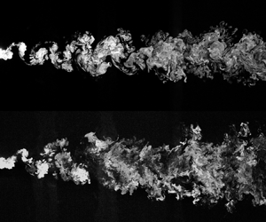
  $1d$ apart from the centre of the cylinder (figure 1a). A low-pass filter is placed in front of the camera lens in order to ignore any laser light noise in the PLIF image. Instantaneous images of the wake in a freestream without and with turbulence are displayed in figures 2(a,b), respectively. The acquisition frequency of the experiment is 100 Hz, and 2000 images were captured for each measurement case.

Figure 1. (a) Conceptual sketch of the experimental set-up. (b) Parameter space ( $TI, L_{12}$) of the background flow in the middle of the field of view at $x/d = 20$.

Figure 2. Visualisation of the wake (a) without (case 1a) and (b) with (case 2a) turbulence present in the background flow.
Following Kankanwadi & Buxton (Reference Kankanwadi and Buxton2020), we employed turbulence intensity ( $TI \equiv \sqrt {(u^2 + v^2)/2}/U_1$, where $u$ and $v$ are velocity fluctuations in the $x$ and $y$ directions, respectively) and integral length scale ( $L_{12} \equiv \int _0^{r_0} R_{12}(r)\,{\rm d}r$, where $R_{12}(r)$ is the correlation coefficient between $u(x,y)$ and $u(x, y+r)$) to characterise the various turbulent background flows, and $r_0$ is the location at which $R_{12}$ first crosses zero. The distribution of the turbulence intensity and the length scale of the flow behind the grids has been documented in detail in Kankanwadi (Reference Kankanwadi2022) in the same facility and operating conditions. The cylinder is placed at various downstream distances from the various grids such that the parameter space $(TI, L_{12})$ was explored as widely as possible in order to truly investigate the behaviour of the interface between the wake and the background flow with various ‘flavours’ of turbulence. We conducted experiments for seven cases of $(TI, L_{12})$, and the distribution of $(TI, L_{12})$ at $x/d = 20$, i.e. the middle of the field of view, is shown in figure 1(b). We divided the seven cases into three groups (figure 1b) according to the magnitude of the turbulence intensity. Case 1a is the closest experimental approximation to a TNTI case with no turbulence-generating grid mounted upstream of the cylinder. The remaining cases are TTI cases with turbulent backgrounds generated by the four different grids and with several different grid–cylinder spacings. In the following sections, each flow configuration case with different $(TI, L_{12})$ is referred to with its corresponding denotation in figure 1(b).
3. Visualisation and determination of the interface
We start with a comparison of the visualisation of the wake of the cylinder in a background flow without (figure 2a) and with (figure 2b) turbulence, thereby featuring the distinction between a TTI and a TNTI. First, in the near wake (say  $x/d \lesssim 10$), the large-scale vortices are more distinct in the case of the non-turbulent background, whilst the locus of the vortices’ positions in the turbulent background extends to a further lateral distance from the wake centreline ( $y = 0$). This confirms the observation of Kankanwadi & Buxton (Reference Kankanwadi and Buxton2023) that the large-scale vortices of the near wake (identified via the velocity field, not the scalar field) in a turbulent background generally drift to further positions in the lateral ( $y$) direction than those in a non-turbulent background at the same $x/d$ location. Second, the TTI is also characterised by a ‘rougher’ boundary with the ambient fluid, at both large and small scales. Large-scale (intermittent) lumps of fluid from the wake are observed protruding into the ambient flow in the turbulent background case (say at $x/d \approx 26$ and 33 in figure 2b), which is barely seen in the non-turbulent background case (figure 2a). It is also noted that there are more finer-scale structures embedded into the TTI, which is likely a reflection of the interaction between the smaller-scale eddies in the ambient turbulence and the interface. The resultant crinkled interface (see also figure 4 for different TTI cases examined) is later demonstrated to have a fractal dimension very different to that of the TNTI, quantifying our observation here that the TTI is ‘rougher’ than the TNTI.
Before proceeding to examine the properties of the interfaces, we need to detect their positions reliably. Both light intensity of the PLIF images (e.g. Westerweel et al. Reference Westerweel, Fukushima, Pedersen and Hunt2009; Gampert et al. Reference Gampert, Boschung, Hennig, Gauding and Peters2014; Mistry et al. Reference Mistry, Philip, Dawson and Marusic2016; Kohan & Gaskin Reference Kohan and Gaskin2022) and the gradient of the light intensity (e.g. Silva & da Silva Reference Silva and da Silva2017; Kankanwadi & Buxton Reference Kankanwadi and Buxton2020) can be used as the threshold quantity in detecting the interface. As the measurement field of view in the present study is relatively large (figure 2), we adopted the light intensity method to avoid the streamwise variation of the threshold value in using the light intensity gradient method. To account for the variation of the light intensity along the streamwise direction in the PLIF images due to mixing/out-of-plane transport (figure 2), the light intensity of each image at each  $x$ position is first normalised by its time-averaged mean value at the same $x$ position along the wake centreline, i.e. $\phi ^*(x,y,t)= \phi (x, y, t)/\bar {\phi }(x, y = 0)$ where the overbar denotes the average over time (images). The resultant normalised images enable a single threshold value to be set for the entire field of view for interface identification purposes (see figures 3b,c).

Figure 3. (a) Distribution of conditionally averaged normalised light intensity  $\langle \phi ^* \rangle$ and ${\mathrm {d} \langle \phi ^* \rangle }/{\mathrm {d} \phi _{th}^*}$ with respect to the threshold $\phi ^*_{th}$. (b) Detected contours using $\phi _{th}^* = 0.3$. (c) Interface lines determined by selecting the longest continuous contours on both sides of the wake. All the result are from case 1a.
In order to determine this threshold, we follow the method used by Prasad & Sreenivasan (Reference Prasad and Sreenivasan1989), who also used PLIF to distinguish the wake from the ambient flow in an experimental configuration similar to our present study. Specifically, for each experimental case (i.e. each data point in figure 1b), a conditional average was taken on the normalised light intensity  $\phi ^*(x,y,t)$ exceeding the given threshold value $\phi _{th}^*$ that reads
 \begin{equation} \langle \phi^* \rangle \equiv \frac{\sum (\phi^*\,|\,\phi^*>\phi_{th}^*)}{N(\phi^*>\phi_{th}^*)} . \end{equation}
The distribution of  $\langle \phi ^* \rangle$ with respect to $\phi _{th}^*$ for the wake with a non-turbulent background is shown in figure 3(a). As expected, $\langle \phi ^* \rangle$ increases rapidly for small values of $\phi _{th}^*$, but there is a knee point of $\langle \phi ^* \rangle$ with respect to $\phi _{th}^*$. This corresponds to the value of the light intensity that well demarcates the limit between the background level of $\langle \phi ^* \rangle$ and that in the wake. The gradient $\mathrm {d} \langle \phi ^* \rangle / \mathrm {d} \phi _{th}^*$ is also plotted in figure 3(a), and a threshold value $\phi _{th}^* =0.3$ was determined with the aid of a linear curve fitting on either side of the knee point. We applied this value to a number of sample images, and it gives a good indication of the position of the interface in the flow. A typical example of the detected interface is given in figure 3(b).
One may note that small occasional patches inside and outside the wake, which result from detrainment, three-dimensional ‘teacup handle’ topology, or engulfment (Westerweel et al. Reference Westerweel, Fukushima, Pedersen and Hunt2009), are also identified. Note that these over-captured patches are disconnected from the continuous interface that we are seeking, so we chose the two longest continuous isocontours corresponding to the threshold criteria, and finally we obtain the interfaces on both sides of the wake (see figure 3c). Typical interface isocontours of all the TTI cases determined using the same method with case-dependent threshold value are displayed in figure 4; all exhibit well-defined interfaces between the wake and the ambient fluids. Comparison of the various figures also highlights beautifully the dependency of the TTI geometry on both  $TI$ and $L_{12}$ of the background turbulence, with clear visual differences across the various cases examined.

Figure 4. Typical interface of all TTI cases: (a) case 1b, (b) case 1c, (c) case 2a, (d) case 2b, (e) case 3a, and (f) case 3b.
Figure 5 further confirms the validation of the interface detection by showing the conditional average of the normalised light intensity  $\langle \phi ^* \rangle _I$ across the detected interfaces in the interface-normal direction (figure 5a). For all cases displayed, this calculation is performed from $x/d = 5$ to $x/d=40$ (figure 5b); only the calculation paths that cross the interface once (the green lines in figure 5a) are considered, to avoid contaminating the result. The clear jump of $\langle \phi ^* \rangle _I$ across the interface ( $\xi = 0$, where $\xi$ is the ordinate on the interface normal; see figure 5a) for all cases manifests as the rapid increase of the light intensity (associated with the dye concentration) from the outer side ( $\xi >0$) to the inner side ( $\xi <0$) of the interface. We also confirm that the profiles of $\langle \phi ^* \rangle _I (\xi )$ retain a clear jump even when the conditional averaging is performed locally in the far wake (e.g. $x/d = 38\unicode{x2013}40$ in figure 5c). It is noted that the nominal interface position ( $\xi =0$), i.e. the isoline of the light intensity corresponding to the threshold value, is slightly (approximately 0.2 mm) dislocated from the start of the light intensity jump, which is due to the marginally higher threshold value (between 0.3 and 0.4 for all cases; see figure 3a) than the background light intensity level (approximately 0.2) so as to differentiate the interface from the noise of the background. It is interesting to see that on the inner side ( $\xi <0$) of the interface, the conditionally averaged light intensity is virtually a constant of order unity, which justifies the normalisation that we adopted for the PLIF images. By using a separate PIV/PLIF combined measurement in the same configuration as the present study (not shown for brevity), we have confirmed that the interface determined from the fluorescent dye well matches the boundary of the wake determined from the vorticity.

Figure 5. (a) Example of an interface segment of case 1a for the conditional average of the light intensity. The green bars normal to the interface show the path along which the conditional average is evaluated and the arrow points to the positive direction in (b) and (c). (b) Conditionally averaged light intensity across the interfaces ( $\xi = 0$, indicated by the dashed line) in the normal direction of all the cases from $x/d = 5$ to $x/d=40$. (c) Conditionally averaged light intensity as in (b) but from $x/d = 38$ to $x/d=40$.
4. Results and discussion
4.1. PDFs of TTI and TNTI positions
After the interface position is determined, the analysis proceeds first with the downstream evolution of the PDFs of both TNTI and TTI positions, which are examined at five different streamwise locations from very near to far away from the cylinder, i.e.  $x/d = 5$, 10, 20, 30 and 40 (figure 6). For presentational clarity, one typical case is displayed for each of the three groups of figure 1(b): figures 6(a,b) are plots of case 1a (the TNTI case), and figures 6(c,d) and 6(e,f) are cases 2a and 3a, respectively (TTI cases). Both of the upper ( $y>0$ in figure 3c) and lower ( $y<0$) interface lines are used in the calculation of the PDF, so a negative value of $y/d$ in figure 6 means the occurrence of a $y>0$ (or $y<0$) interface on the $y<0$ (or $y>0$) side at the examined $x/d$ position. The PDF at a particular $x/d$ position was calculated within a streamwise strip of extent $3d$ centred on $x_c$ as denoted in the figure. The $3d$ extent of these strips is comparable to the largest integral length scale within the background flow (see figure 1b), and enabled better statistical convergence when computing the PDFs.

Figure 6. Streamwise development of PDFs of both TNTI and TTI positions: (a,b) TNTI case 1a, (c,d) TTI case 2a, and (e,f) TTI case 3a.
For the examined TTI cases (figures 6c,e), the modal peak of the PDF, i.e. the most probable position of the interface that is very close to the mean position of the interface, is roughly at the same position as that of the TNTI case (figure 6a) at  $x/d = 5$ (marked by the left-hand dashed line). However, at $x/d = 40$ (marked by the right-hand dashed line), the position $y/d$ of the modal location of the TTI is larger than that of the TNTI, especially when the background turbulence intensity is high (figure 6e). Kankanwadi & Buxton (Reference Kankanwadi and Buxton2023) showed that in the near-wake region ( $x/d \leq 5$), the wakes exposed to background turbulence were always wider on average than the wake embedded in a non-turbulent background. Our results show that in the near wake, the modal position of the TTI is similar to the TNTI, and the reason why the mean wakes are wider for the TTI cases is because of the diminished contribution from the left tails of the PDFs (e.g. PDFs for $x_c = 5$ in figures 6a,c,e), i.e. there are fewer instances of the TTI crossing the centreline than the TNTI doing so. This observation is consistent with the finding in Kankanwadi & Buxton (Reference Kankanwadi and Buxton2023) that the mean position of the centres of the von Kármán vortices for the TTI cases were further away from the wake centreline than those of the TNTI case at the same streamwise position. Further, our results show that the increase in wake width in the presence of background turbulence extends to the far wake, up to the $40d$ position examined in the present study, with the intensity of the background turbulence seemingly the most important parameter in determining this enhanced wake width. Later, we will see that this average enhancement of the wake width comes mainly from the contribution of the region closer to the cylinder, which then persists downstream.
It is noted that the TTI position PDFs for two cases with background turbulence (figures 6c,e) are not Gaussian, with a negative skewness (not shown) over all the examined  $x/d$ range; a similar observation was also made by Kohan & Gaskin (Reference Kohan and Gaskin2022) for the TTI position of an axisymmetric jet. The PDF of the TNTI position is practically Gaussian at $x/d = 40$ (shown later, in figure 9), which has been reported widely in previous literature in fully developed regions of turbulent flows (e.g. Corrsin & Kistler Reference Corrsin and Kistler1955; da Silva et al. Reference da Silva, Hunt, Eames and Westerweel2014; Mistry et al. Reference Mistry, Philip, Dawson and Marusic2016; Zhou & Vassilicos Reference Zhou and Vassilicos2017). However, the TNTI PDF evidently deviates from a Gaussian distribution at positions closer to the cylinder, especially at $x/d = 5$ and 10 (figure 6a) where heavier negative tails than for a Gaussian PDF are displayed. These distinctly heavy negative tails reflect the high probability of the interface appearing on the opposite side of the wake centreline ( $y/d = 0$), which is a manifestation of the strong large-scale ‘meandering’ of the near wake (see figure 2) because of the coherent vortices (e.g. Chen et al. Reference Chen, Zhou, Zhou and Antonia2016; Kankanwadi & Buxton Reference Kankanwadi and Buxton2023).
Zhou & Vassilicos (Reference Zhou and Vassilicos2017) found that the PDF of the TNTI position in a turbulent, axisymmetric wake scales with the wake width in the self-preserving region. Such an observation is not made in the current study as shown in figures 6(b,e,f), where the PDFs of both TNTI (figure 6b) and TTI (figures 6e,f) positions are normalised with the wake half-width  $L_{\phi }(x)$ estimated from the mean profile of the light intensity $\bar {\phi }(x, y)$ of the PLIF images at the corresponding $x$ position. Here, we use the wake half-width determined from the mean scalar profiles instead of the mean velocity profiles to represent the local characteristic length scale of the wake, mainly because the velocity half-width is not well-defined for the cases with a turbulent background. In particular, the inhomogeneity in the mean flow of the background turbulence generated by the fractal grids (cases 1b, 1c and 2b in figure 1) contributes to the difficulty of determining the boundary of the mean velocity (and hence the maximum mean velocity deficit) of the wake. In fact, $L_{\phi }(x)$ is shown to scale with the local velocity wake half-width for the wake with a non-turbulent background flow (see the Appendix). The normalised PDFs of both TNTI and TTI positions for all cases assessed do not collapse but exhibit an evident streamwise evolution. This is not unexpected as the PDFs of either TTI or TNTI position in the current flow region are, as discussed in the previous paragraph, affected heavily by the large-scale coherent vortices, and are not self-similar, as manifested by the heavy negative tails at $x/d = 5$ and 10. What is interesting to see is that the most probable TTI and TNTI positions do scale approximately with the local $L_{\phi }$, which provides a straightforward way to estimate the most probable positions for both TNTI and TTI, even though the PDFs are not self-similar.
The coincidence of the modal peaks in figures 6(b,d,f) coupled to the Gaussian-like nature of the PDFs for the further downstream locations suggests that the mean position of the interface  $\overline {y_I}(x)$ at different $x/d$ positions may scale with the local wake half-width. This is confirmed in figure 7 for both the TNTI case and all the TTI cases. Figure 7(a) first compares the streamwise evolution of $\overline {y_I}(x)$ for both TNTI (case 1a) and TTI cases scaled with the cylinder diameter $d$. It is clear that all the TTI cases have a larger mean value of $\overline {y_I}$ than the TNTI case at almost all $x/d$ positions, which is consistent with the observation in figures 6(a,c,e). It seems that the turbulence intensity is the dominant parameter in determining the mean position of the TTI, as there is little evident distinction between the TTI cases within groups 1 and 2, in which integral length scale is the major differentiating factor. What should be noted is that the mean interface position at a particular $x/d$ location reflects mainly the mass entrainment accumulated upstream of $x/d$, whilst the slope of the curve $\mathrm {d} \overline {y_I} / \mathrm {d}\kern 0.06em x$ demonstrates the local entrainment rate into the wake (Kankanwadi & Buxton Reference Kankanwadi and Buxton2023). It is found that in figure 7(a), there is an apparent turning point of the slope of $\overline {y_I}(x)$ located at $x/d \approx 15$, after which $\overline {y_I}(x)$ grows noticeably more slowly than farther upstream, for both TNTI and TTI cases. It indicates that the entrainment rate upstream of $x/d \approx 15$ is faster than after this position. We also notice that in the flow region $x/d \lesssim 15$, the mean interface position $\overline {y_I}(x)$ of the TTI cases grows almost linearly and at a faster rate than the TNTI case; a similar observation was made by Kankanwadi & Buxton (Reference Kankanwadi and Buxton2023) in the flow region very close to the cylinder ( $x/d \leq 5$). It is thus concluded that the turbulence in the background promotes spreading of the wake boundary mostly in the near wake region (say $x/d < 15$); It is interesting to see that the turning point at $x/d \approx 15$ is almost the same for all cases tested, regardless of whether there is a TNTI or a TTI. Although the physics underpinning the changes of the slope of $\overline {y_I}(x)$ is still unclear, it is surmised that this transition position may depend on the dynamics of the near-wake coherent vortices that have been reported to be important for near-wake large-scale engulfment (Kankanwadi & Buxton Reference Kankanwadi and Buxton2023), and decays significantly from $x/d = 10$ to $x/d=20$ at a similar Reynolds number (e.g. Zhou et al. Reference Zhou, Zhou, Yiu and Chua2003; Chen et al. Reference Chen, Zhou, Zhou and Antonia2016; and also the visualisation in figure 2). After this turning point, the growth of the wake likely transitions from being large-scale engulfment-driven entrainment to small-scale nibbling-driven entrainment

Figure 7. Streamwise distribution of the mean interface positions (a)  $\overline {y_I}/d$ and (b) $\overline {y_I}/L_\phi$ of all cases.
When the mean interface position is scaled by  $L_\phi$ (figure 7b), all $\overline {y_I}/L_\phi$ become approximately constant after an initial development region ( $x/d \lesssim 15$). This is consistent with the observation in figure 6 that the most probable position of $y_I$ scales with $L_\phi$, which itself follows a power-law scaling while developing downstream (figure 8). Eames, Jonsson & Johnson (Reference Eames, Jonsson and Johnson2011) developed a model that describes how a wake spreads in a highly turbulent flow. They pointed out that for two-dimensional bodies, the wake grows linearly with distance during the initial development region (Eames et al. (Reference Eames, Jonsson and Johnson2011) called it ‘the ballistic regime’) until the wake width is comparable to the integral scale of the background turbulence, beyond which the wake width grows diffusively with a scaling $\sim x^{1/2}$. Typical examples seeking a power-law scaling for $L_\phi \sim x^\alpha$ are displayed in figure 8. After $x/d \approx 10$, the scaling $L_\phi \sim x^{1/2}$ is indeed observed in almost all cases with a turbulent background, with the scaling exponent varying as $0.48 \leq \alpha \leq 0.54$, except for two cases (case 1c and 2a in figure 2, with scaling exponents 0.64 and 0.23, respectively). It is noted that for the non-turbulent background case (group 1a), the scaling exponent (0.35) is close to $1/3$, rather than the value ( $1/2$) expected based on the self-similarity, which is achieved only in the very far wake (say $x/d = 200$ in Chapter 4 of Tennekes & Lumley Reference Tennekes and Lumley1972).

Figure 8. Streamwise distribution of the wake half-width  $L_\phi$ with turbulent (cases 2b and 3b) and non-turbulent (case 1a) background flow.
We close the discussion of this section with a comparison between the centred PDF of  $y_I$ for all the examined TNTI and TTI cases (i.e. the PDF of $(y_I-\overline {y_I})/\sigma _I$, where $\sigma _I$ is the standard deviation of $y_I$) and a standard Gaussian distribution (figure 9), so as to highlight the different extents to which the TNTI and TTI position PDFs deviate from Gaussianity as $x/d$ varies. It is clear that very close to the cylinder at $x/d = 5$ (figure 9a), the PDFs of both TNTI (case 1a) and all TTI cases deviate from the Gaussian distribution significantly with evident negative skewness, as is also seen in figure 6. Of note is that as $x/d$ increases, the negative skewness of the TNTI position gradually reduces and the PDF becomes essentially Gaussian at $x/d = 40$ (figure 9d), whilst the PDFs for all the TTI cases still deviate from Gaussianity, although the skewness does reduce as $x/d$ increases. It is clear that for both TNTI and TTI cases, the dynamics in the near wake (figure 2) is very different from that farther downstream, where the large-scale coherent vortices have largely dissipated and the turbulence becomes fully developed.

Figure 9. Comparison of centred PDFs of TNTI and all TTI cases at different  $x/d$ positions: (a) $x/d = 5$, (b) $x/d=10$, (c) $x/d=20$, and (d) $x/d=40$.
Previous literature examining the TNTI position in turbulent jets (e.g. Westerweel et al. Reference Westerweel, Fukushima, Pedersen and Hunt2009; Watanabe et al. Reference Watanabe, Sakai, Nagata, Ito and Hayase2014; Mistry et al. Reference Mistry, Philip, Dawson and Marusic2016) has also reported the slight deviation of the TNTI position PDF from a Gaussian distribution with small, non-zero skewness. This implies that extreme interface positions occur in one direction with a higher probability than in the other direction. Such large interface position displacements from the jet centre are unlikely to be caused by the small-scale turbulent motions within the jet. We identify similar non-Gaussian TNTI position PDFs for turbulent wakes (as well as for TTIs), e.g.  $x/d = 5$ in figure 9(a). Further downstream, where the large-scale coherent motions have largely dissipated, the TNTI-position PDF resorts to a Gaussian distribution (e.g. $x/d = 40$ in figure 9d). Jets also experience a spatial evolution, with large-scale coherent motions embedded in the region near the jet exit (Ball, Fellouah & Pollard Reference Ball, Fellouah and Pollard2012), which subsequently decay with streamwise distance. Our results support unequivocally the conclusion that as the wake's coherent motions decay, the TNTI position PDF resorts from a non-Gaussian distribution to Gaussianity. Given the similar spatial decay of the coherent motions in axisymmetric jets, this lends support to the notion that non-Gaussian TNTI position PDFs are associated with the presence of energetic coherent motions, regardless of flow type.
The different dynamics in the near and relatively far wake are believed to lead to distinct geometrical features of the interfaces (TNTI and TTIs), which encourages us to investigate the fractal dimension of the interfaces, and their spatial evolution, in the next subsection.
4.2. Fractal dimension of the TNTI and TTI
As explained in the Introduction, the multi-scale self-similar geometric features of the interface, either TNTI or TTI, can be described with fractal analysis, which was first demonstrated by Sreenivasan & Meneveau (Reference Sreenivasan and Meneveau1986). The length of a fractal ‘line’ follows a power law with increased resolution scale  $r$, namely,
 \begin{equation} L_I(r) \sim r^{1-D}, \end{equation}
where  $D$ is the fractal dimension, which has been reported to be between 1.3 and 1.4 for a TNTI (e.g. Prasad & Sreenivasan Reference Prasad and Sreenivasan1989; de Silva et al. Reference de Silva, Philip, Chauhan, Meneveau and Marusic2013; Abreu, Pinho & da Silva Reference Abreu, Pinho and da Silva2022), while for the TTI the dimension is somewhat higher and an increasing function of the turbulence intensity in the ambient flow (Kankanwadi & Buxton Reference Kankanwadi and Buxton2020; Kohan & Gaskin Reference Kohan and Gaskin2022). However, these previous studies focus on the TTI in the fully developed region of a turbulent flow, where Kankanwadi & Buxton (Reference Kankanwadi and Buxton2020) demonstrated that the turbulent length scale in the ambient flow has little effect on the fractal dimension of the interface. In the previous subsection, we have shown that the behaviour of the interfaces is influenced substantially by the strong organised motions in the near wake. As we have measured multiple cases of TTIs with various levels of turbulence intensity and integral length scales in the background flow, it is of interest to examine the fractal dimension of these TTIs in the context of the streamwise decay of the coherent vortices.
To obtain the fractal dimension of the interfaces, we adopt a ‘filtering method’ as used in previous studies (e.g. de Silva et al. Reference de Silva, Philip, Chauhan, Meneveau and Marusic2013; Kankanwadi & Buxton Reference Kankanwadi and Buxton2020; Abreu et al. Reference Abreu, Pinho and da Silva2022). Specifically, each PLIF image is filtered with a box filter of different sizes  $\varDelta _f$ between $0.1d$ and $1.6d$; an interface is determined after each filtering, and the threshold of the light intensity used to identify the interface is kept the same for all interface determination. Consequently, the identified interface gets progressively smoother with resolution scale smaller than the filtering size smeared (figure 10a). The lengths of the interface corresponding to a particular resolution size (i.e. the filter size) $L_I(r = \varDelta _f)$ are obtained. Note that there are two lines on both sides of the wake, whose lengths are calculated separately, and both are included in the ensemble to calculate the mean length of the interface line. Based on (4.1), $\log (L_I)$ has a linear relationship with $\log (r)$ when such a scaling applies, and the slope of the line (i.e. $1-D$, referred to as the scaling exponent in the following text) is related directly to the fractal dimension. Figure 10(b) displays a distribution of the mean turbulent/non-turbulent interface length of all detected realisations with respect to different filter sizes. In the scale range between $0.2d$ (close to the Taylor microscale on the wake centreline at $x/d = 20$ of the TNTI case, estimated from Kankanwadi Reference Kankanwadi2022) and 1 $d$, a scale comparable to the integral length there is a strong linear fit between $\log (\overline {L_I}/d)$ and $\log (\varDelta _f/d)$, with slope of the fitted line $-$0.34. This yields a fractal dimension $D = 1.34$ for the TNTI, which agrees well with the value in previous reports, e.g. 1.36 in Prasad & Sreenivasan (Reference Prasad and Sreenivasan1989), 1.3 in de Silva et al. (Reference de Silva, Philip, Chauhan, Meneveau and Marusic2013), and $1.36 \pm 0.03$ in Wu, Zaki & Meneveau (Reference Wu, Zaki and Meneveau2020).

Figure 10. (a) Filtered interface with different filter scales (case 1a). (b) Scaling of the length of the interface  $\overline {L_I}$ in (a). (c) Fractal dimension of the interface obtained using different window widths for cases 1a and 3b at $x/d = 20$. The vertical dashed line indicates the window width used for calculating the local fractal dimension of the interface.
To compute the local fractal dimension of the interfaces at different  $x/d$, we must choose a ‘window’ covering a finite length of the whole interface; the window span should be large enough to produce a good representation of the local interface's fractality, but small enough to ensure homogeneity over the streamwise extent of the window, and yielding good spatial resolution for the fractal dimension's distribution (with respect to $x/d$). Figure 10(c) shows the distribution of the scaling exponent ( $1-D$), determined in the same way as exhibited in figure 10(b), with respect to different streamwise window extents. Two typical cases are examined with the window centre set at $x/d = 20$: the TNTI case 1a, and the TTI case 3b, which has the highest turbulence intensity in the ambient flow (figure 1b). The value $1-D$ for both cases shows a weak increasing trend as the window span grows; there is a narrow plateau between window spans $7d$ to $11d$, displaying a reasonable value $-$0.36 (e.g. Prasad & Sreenivasan Reference Prasad and Sreenivasan1989). We therefore chose a window span $8d$ corresponding to the beginning of the plateau in the following study for the best spatial resolution of the results.
Figure 11 shows the scaling of the mean length of the filtered interface of the TNTI case with respect to the scale of the filter at various streamwise positions. In the figure,  $x_c/d$ located between 4 and 40 is the centre position of the examination window with span $8d$. There is a well-defined scaling range between $\varDelta _f/d = 0.2$ and $\varDelta _f/d=1$ for all the examined positions, although the scaling range is wider in the larger scale end for positions closer to the wake generator. It is interesting to see that the slope of the fitted line ( $= 1-D$) varies from $-$0.28 in the very near wake to an oft-reported $-$0.37 at $x_c = 40$, indicating that there is indeed an essential difference in the geometric features of the interface in the near wake and the fully-developed downstream positions. To explore the effect of the background turbulence on the fractal features of the interfaces, we summarised the streamwise distributions of the scaling exponent of all the measured cases in figures 12(a,b), in which the effects of the background turbulence intensity and length scale on the fractal dimension are examined, respectively.

Figure 11. Scaling of the interface length of the TNTI case using window width  $8d$ at different streamwise $x/d$ positions.

Figure 12. Streamwise distribution of fractal dimensions of TNTI and all TTI cases: (a) effect of turbulence intensity, and (b) effect of integral length scale.
In figure 12(a), the streamwise distributions of the scaling exponent  $1-D$ of cases 2a, 3a and 3b, which are TTI cases with relatively small integral scale and large turbulence intensity in the background flow (figure 1b), are compared with that of the TNTI case (case 1a). The TNTI case exhibits a constant value approximately $-$0.36 in the region $x/d \gtrsim 10$; the three TTI cases have similar distributions of $1-D$ to the TNTI case before $x/d \approx 15$, which, interestingly, corresponds to the position where the wake spreading rate decreases evidently (figure 7a). After this $x/d$ position, the scaling exponent of the TTI cases continues to increase in magnitude and reaches approximately $-$0.45 at $x/d = 40$. The larger TTI fractal dimension than that of the TNTI is also consistent with the observation of Kohan & Gaskin (Reference Kohan and Gaskin2022) in an axisymmetric jet with a turbulent background. The growing $1-D$ of the TTIs relative to the TNTI in the far field of the wake indicates that the turbulence intensity in the background flow becomes gradually essential in determining the fractal dimension of the interface in the positions far from the wake generator. The increased fractal dimension in the far field of the wake can also be observed in the visualisation in figure 2(b), in which the boundary of the wake becomes ‘rougher’ (i.e. a larger fractal dimension) as the flow proceeds downstream, with intermittent lumps and also finer structures. These structures result from the interactions between the eddies in the background turbulence and those of the wake. In the region closer to the cylinder before $x/d \approx 15$, the ambient turbulence does not differentiate the scaling exponent of the TTIs from the TNTI. It implies that in this flow region, which features the evolution of the strong von Kármán vortices, the fractal nature of the interface is determined mainly by the dynamics of the wake flow itself, at least when the scale of the energetic eddies in the ambient flow is not overpowering (as is the situation in cases 2a, 3a and 3b).
In figure 12(b), the TTI cases 1b and 1c, which possess low turbulence intensity and increasing integral length scale in the background flow, are compared with the TNTI case (case 1a); case 2b, which has a large integral length scale and also higher turbulence intensity, is also added for comparison. In contrast to the similar distribution of different cases upstream of  $x/d \approx 15$ in figure 12(a), the scaling exponent distributions of the compared cases show evident scatter in the upstream region but gradually converge to a value ${\approx }-0.36$ in the downstream flow. TTI cases 1b and 1c differ from the TNTI case 1a mainly in the integral length scale of the background flow; their distinctive $1-D$ distributions in the upstream region indicate that the integral scale of the background turbulence is of great importance to the fractal dimension of the interfaces in this region. Compared to the TNTI case, the TTI case 2b has both a higher turbulence intensity and a larger integral length scale (figure 1b), and its distribution is not significantly different from that of the TNTI case in both the upstream and downstream fields. It seems that there is a compound effect of the background turbulence intensity and the integral length scale on the interface geometry. As a matter of fact, such a combined effect was reported by Kankanwadi & Buxton (Reference Kankanwadi and Buxton2020, Reference Kankanwadi and Buxton2023) in the same flow: in the upstream field, both the turbulence intensity and integral length scale in the background flow act to enhance the entrainment rate into the wake, whilst only the turbulence intensity of the background turbulence is important in suppressing entrainment in the downstream field.
To summarise the discussion of figure 12, generally, both turbulence intensity and integral length scale in the background flow have an effective influence on the fractal dimension of the interface, and in different regions of the flow, a different parameter is in dominance. In the near wake, the integral length scale is the more important parameter; as the flow develops downstream, with the coherent vortices degrading substantially, the effect of the integral length scale weakens, and the influence of the turbulence intensity gradually prevails. This observation is consistent with the conclusion obtained in the TTI entrainment studies of Kankanwadi & Buxton (Reference Kankanwadi and Buxton2020, Reference Kankanwadi and Buxton2023) that integral length scale is the more important parameter in the near wake, which promotes the large-scale engulfment of the wake, whilst the turbulence intensity suppress the small-scale ‘nibbling’ in the far field where the integral scale is of less relevance.
5. Summary and conclusions
We examined the spatial evolution of the geometry of the interface of a turbulent cylinder wake from the near field ( $x/d = 5$) to the relatively far field ( $x/d = 40$), in a turbulent background with various levels of turbulence intensity and integral length scale (figure 1b). A PLIF experiment was carried out to capture the interface between the wake and the turbulent background flow. Attention was paid to the streamwise evolution of the geometric properties of these TTIs and a TNTI reference case, including their PDFs, scaling and fractality, in the context of the large-scale vortices gradually diminishing in the wake.
Compared to the conventional TNTI, the TTI spreads faster towards the ambient flow as the wake develops downstream, which is due mainly to the enhanced rate of entrainment in the near wake (Kankanwadi & Buxton Reference Kankanwadi and Buxton2023). We find a transition region of the interface spreading outwards at  $x/d \approx 15$, after which the interfaces spread at an evidently reduced rate (figure 7a). It is conjectured that the different spreading rates before and after this transition region are associated with the dynamics of the large-scale coherent vortices, which induce strong engulfment (Kankanwadi & Buxton Reference Kankanwadi and Buxton2023; also visualisation in figure 2) and decay rapidly from $x/d = 10$ to $x/d=20$ at similar Reynolds numbers (e.g. Zhou et al. Reference Zhou, Zhou, Yiu and Chua2003; Chen et al. Reference Chen, Zhou, Zhou and Antonia2016). After this region, the mean positions of the interfaces, including both TNTI and all TTI cases, display a reasonable scaling with the wake half-width $L_\phi$ (figure 7b). We find that $L_\phi$ agrees well with the Eames et al. (Reference Eames, Jonsson and Johnson2011) theoretical downstream evolution scaling $(x/d)^{1/2}$ in a turbulent background. It is interesting to see that this transition region is roughly the same for both TNTI and TTI cases examined, suggesting that this transition region is robust and not dependent on the turbulence in the background flow, at least for the turbulence intensity and length scale range examined in the present study.
It is noted that the PDFs of both TTI and TNTI positions are not Gaussian in the near wake (especially for  $x/d \lesssim 10$), with evident negative skewness that reflects the ‘deep-diving’ interface towards the wake central region due to the strong engulfment by the coherent vortices at these locations (figure 2). This observation is distinctly different from the oft-reported Gaussian distribution of TNTI position at locations of fully developed turbulence in the absence of dominant coherent motions (e.g. da Silva et al. Reference da Silva, Hunt, Eames and Westerweel2014; Mistry et al. Reference Mistry, Philip, Dawson and Marusic2016; Zhou & Vassilicos Reference Zhou and Vassilicos2017; and also the Gaussian PDF of TNTI position at $x/d = 40$ in figure 9d). Note that the PDFs of TTI position still depart from Gaussianity with a slight negative skewness even at $x/d = 40$ (figure 9d), which agrees with the observation of Kohan & Gaskin (Reference Kohan and Gaskin2022) of the TTI in a fully-developed axisymmetric jet.
We found that the fractal dimension of the TTIs in the near and relatively far wake are dictated by different parameters of the background turbulence. Turbulence intensity induces a higher fractal dimension of the interface in the far wake. It is highly likely to be resultant from the interaction between the ambient eddies and those of the wake near the interface, which can be observed partly from the evident intermittent small-scale structures on the interface of the wake in turbulence background in figure 2(b). The effect of the integral length scale is more appreciable in the near wake region (figure 12b). Kankanwadi & Buxton (Reference Kankanwadi and Buxton2023) show that the freestream turbulence with large integral length scale can significantly increase the transverse location of the centres of the von Kármán vortices in the near wake ( $x/d < 5$) relative to the centreline. Therefore, we have reason to expect that the energetic eddies of the background flow interact with the coherent vortices in the near wake, in which only the energetic eddies in the background flow with comparable length scale or turnover time would interact effectively with the coherent vortices in the wake. This is likely the reason why background integral scale is important in the near wake. Such large-scale interactions in the near wake would not necessarily wrinkle the interface, as the small-scale interaction does in the far wake, explaining why cases with larger integral scale do not necessarily cause higher fractal dimension of the interface (figure 12b). Such large-scale interaction would be expected to cause large-scale oscillation or meandering of the wake, however, which has been demonstrated by Kankanwadi & Buxton (Reference Kankanwadi and Buxton2023).
Finally, some comments about future studies are worthwhile. The interaction between the background turbulence and the wake is certainty three-dimensional. The anisotropy of the turbulent scales in the background could cause different levels of distortion of the interface in the streamwise and spanwise directions, which can lead to different behaviour of the fractality of the interface in the two directions. This is an interesting topic to be addressed in future studies, either via direct numerical simulations or by imaging the wake in planes of different  $x/d$.
Funding
The authors would like to acknowledge the Engineering and Physical Sciences Research Council for funding the work under grant no. EP/V006436/1.
Declaration of interests
The authors report no conflict of interest.
Appendix. Determination of  $L_\phi$

This appendix is added to show how the wake half-width  $L_\phi$ of the scalar field is determined based on the PLIF measurements and its connection with the velocity wake half-width $L_u$.
The profiles of the typical cases of the time-averaged light intensity of the PLIF images  $\bar {\phi }(y)$ at $x/d = 5$–40 are shown in figure 13. It is noted that the mean concentration of the fluorescent dye in the flow field is quite low, thus the fluorescent response is effectively a linear function of the dye concentration (Crimaldi Reference Crimaldi1997; Vanderwel & Tavoularis Reference Vanderwel and Tavoularis2014; Baj, Bruce & Buxton Reference Baj, Bruce and Buxton2016); thus $\bar {\phi }(y)$ can be treated virtually as the concentration of the dye, which is confirmed in figure 14. For all the cases considered (figures 13a,c,e,g), $\bar {\phi }(y)$ decays reasonably in magnitude and spreads into a wider range as $x/d$ increases. Similar to the definition of velocity wake half-width, the scalar wake half-width $L_\phi$ is defined such that $\bar {\phi }(y = L_\phi ) = 1/2\,\bar {\phi }(y = 0)$. It is interesting to find that the streamwise evolution of $\overline {\phi ^*}$ scales well with $L_\phi$ for all the TTI cases (figures 13d,f,h); for the TNTI case (figure 13b), $L_\phi$ also works well for $x/d \geq 20$. It seems that the scalar field of the wake in a turbulent background becomes self-preserving at a smaller $x/d$ position than that in a non-turbulent flow. A similar observation for the velocity field was also made by Eames et al. (Reference Eames, Jonsson and Johnson2011).

Figure 13. Profiles of mean light intensity of PLIF images of typical cases: (a,b) TNTI case 1a, (c,d) TTI case 1c, (e,f) TTI case 2a, and (g,h) TTI case 3b.

Figure 14. Ratio of scalar wake half-width  $L_\phi (x)$ to velocity wake half-width $L_u(x)$ at different $x/d$ positions of a cylinder wake.
To the best of our knowledge, there is no published theoretical prediction for the similar behaviour of  $L_\theta$ and $L_u$ in wakes. However, it is reasonable to envisage that there must be an interlink between $L_\theta$ and $L_u$, since the distribution of the scalar is determined passively by the velocity field. This is confirmed in the present measurement of the non-turbulent background case shown in figure 14, in which the ratio $L_\phi /L_u$ is observed to be approximately constant at $x/d \geq 20$. Here, $L_u$ is the wake half-width determined from the mean velocity profile of our non-published particle image velocimetry measurement of the cylinder wake without grids upstream. Note that a similar result was obtained in the measurements of Chen et al. (Reference Chen, Zhou, Zhou and Antonia2016) and Zhou, Zhang & Yiu (Reference Zhou, Zhang and Yiu2002) in the wake of a cylinder at the same $x/d$ range, except that their passive scalar was represented by temperature in the flow. The slightly larger value of the present measurement could possibly be attributed to the different initial conditions to those of the two references: in our experiment, the dye is released from a hole in the rear surface of the cylinder, while the scalar (heat) in Chen et al. (Reference Chen, Zhou, Zhou and Antonia2016) and Zhou et al. (Reference Zhou, Zhang and Yiu2002) is injected from the shear layer of the wake by heating the cylinder electrically; in addition, the Schmidt number for the fluorescent dye (approximately 2500; see § 2) is much larger than the Prandtl number (approximately 0.7) of heat in air, which can also cause the scalar to be diffused distinctly (e.g. Rehab, Antonia & Djenidi Reference Rehab, Antonia and Djenidi2001). The resemblance between our measurements and those from Chen et al. (Reference Chen, Zhou, Zhou and Antonia2016) and Zhou et al. (Reference Zhou, Zhang and Yiu2002) confirms our expectation that the distribution of the mean value of the fluorescent intensity is a reasonable representation of the distribution of the mean scalar concentration.


