


1. Introduction
Spray atomization has a wide variety of applications ranging from the manufacturing of pharmaceuticals to the production of metal powders for use in additive manufacturing. Despite the prolific and long-running use of sprays in industry, the understanding of the atomization process is not yet well enough understood to attain good prediction of the variety of sizes of droplets produced by the spray when varying the working fluids or the nozzle design and scale. A commonly used nozzle type is the twin-fluid nozzle, which exploits a high-velocity gas flow to disturb and fragment a liquid jet. The simplest form of twin-fluid nozzle is the coaxial configuration, where a central liquid jet of diameter  $d_l$ moving at a relatively low speed, $u_l$, is surrounded by an annular sheath of high-speed gas, moving at $u_g$ with thickness $b_g$. The resulting aerodynamic interaction is dependent on the nozzle geometry ( $d_l$ and $b_g$), its operation ( $u_g$ and
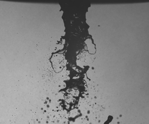
  $u_l$) and the liquid and gas phase properties. Images depicting the twin-fluid spray breakup are shown in figure 1. The aerodynamic disturbance of the liquid jet results in its fragmentation into a range of droplet sizes, commonly represented by a droplet size frequency distribution, $f$, and often characterized by representative mean sizes such as the Sauter mean diameter, $d_{32}$, in $\mathrm {\mu }$m. Studies on twin-fluid atomization primarily seek to understand and predict $f$ and $d_{32}$ for sprays.

Figure 1. Images of a typical twin-fluid spray; 2850-70 nozzle operating at  $G_l = 526$ kg m $^{-2}$ s $^{-1}$ with (a) $G_g = 210$ kg m $^{-2}$ s $^{-1}$ and (b) $G_g = 319$ kg m $^{-2}$ s $^{-1}$.
Empirical studies of coaxial, twin-fluid sprays have primarily focused on developing correlations for  $d_{32}$. One of the earliest of such correlations is that of Nukiyama & Tanasawa (Reference Nukiyama and Tanasawa1950), who showed that the $d_{32}$ correlates well to the summation of two terms; one that captures the interplay of gas velocity and surface tension and one that relates to the liquid viscosity. However, the developed correlation was not dimensionally consistent; thus, later works such as Rizk & Lefebvre (Reference Rizk and Lefebvre1983) expanded upon this original correlation to make it non-dimensional, where the first and second terms are represented by the Weber, $We$ and Ohnesorge, $Oh$, numbers, given by
 \begin{equation} We = \frac{\rho_g u_r^2 d}{\sigma} \end{equation}
and
 \begin{equation} Oh = \frac{\mu_l}{\sqrt{\rho_l \sigma d}}, \end{equation}
respectively, where  $\rho _g$ and $\rho _l$ are the gas- and liquid-phase densities in kg m $^{-3}$, $\mu$ is the liquid viscosity in Pa s, $\sigma$ is the interfacial surface tension in N m $^{-1}$, $u_r$ is the relative velocity between the gas and the droplet in m s $^{-1}$, and $d$ is a characteristic diameter, usually taken as the diameter of the liquid jet or the liquid jet orifice, $d_l$. The effects of the liquid flow rate are often represented in terms of the liquid jet Reynolds number, $Re_l$, the liquid-to-air mass flow ratio, $m_r$, or the momentum-flux ratio, $M$, defined as
 \begin{equation} Re_l = \frac{\rho_l u_l d}{\mu_l},\quad m_r = \frac{\dot{m}_l}{\dot{m}_g},\quad M=\frac{\rho_g u_g^2}{\rho_l u_l^2}. \end{equation}
 In many correlations,  $m_r$ and $M$ are used to weigh the contributions of the $We$ and $Oh$ terms to capture the effect of the liquid flow on the atomization. Since the scaling of such correlations is based only on fitting to a dataset, such correlations do not provide a good understanding of the underlying mechanisms of the atomization. While the simple correlations that result from empirical models are useful in industry for process control and optimization, they are inherently only valid for the fluids, nozzles and operating conditions for which they are tuned, making them less useful for extrapolative prediction such as process scaling. Furthermore, they provide only a cursory understanding of the fundamental dynamics of atomization. As a result, their practical use is limited to parameter spaces that have already been extensively probed experimentally and cannot be used effectively to inform process or nozzle design.
One of the challenges of using empirical correlations for twin-fluid atomization is that it exhibits varied phenomenology depending on the operating conditions, which are often referred to as the morphologies of the spray. As a result, any correlation or model should be developed for a specific morphology or contain allowances for the varied morphologies. The boundaries of these morphologies for twin-fluid, coaxial nozzles are generally classified in terms of  $We$ (the gas jet condition) and $Re_l$ (the liquid jet condition). In most twin-fluid nozzle applications, where $We$ is high and $Re_l$ is low, the relevant morphologies are membrane and fibre-type breakup. The former is characterized by the formation of bags and occurs at relatively low $We$, while the latter is characterized by the peeling of fibres off of the liquid jet at relatively high $We$, as shown in figures 1(a) and 1(b), respectively. These morphologies are analogous to the breakup morphologies of droplets, where membrane and fibre-type breakup correspond to the bag-type (bag, bag & stamen and multibag) and sheet-thinning morphologies, respectively. As with most multiphase flow regime maps, the morphology transition boundaries are not exact. Additionally, they will depend on how the axes are defined. In earlier maps, such as in Chigier & Farago (Reference Chigier and Farago1992), the $We$ axis is based on the relative speed of the air stream to the liquid stream, $u_r$, while in more recent maps, such as in the review of Lasheras & Hopfinger (Reference Lasheras and Hopfinger2000), it is based instead on $u_g$ only, resulting in slightly different boundaries. In maps utilizing $u_r$, the transition from the membrane to the fibre type occurs at $We \approx 80$, while in maps utilizing $u_g$, the transition occurs in the range $100 < We < 300$, depending on $Re_l$. The boundary in terms of $u_r$ of $We \approx 80$ strengthens the analogue to the droplet breakup case, where the transition from the bag-type to the sheet-thinning morphology occurs at the same condition (Guildenbecher, López-Rivera & Sojka Reference Guildenbecher, López-Rivera and Sojka2009). Note that the use of $u_r$ is more accurate to the underlying physics while using $u_g$ is more convenient for separating the gas and liquid flow effects.
It is worth noting that these morphologies were identified based on what would now be considered quite low resolution imaging, both spatially and temporally, which was also the case previously with the breakup morphologies of droplets. The sheet-thinning morphology, for example, was previously identified as boundary layer stripping, which described the stripping of droplets directly from the periphery of the parent droplet due to the high shear force (Ranger & Nicolls Reference Ranger and Nicolls1969). However, later investigations utilizing higher resolution imaging revealed that a rim and sheet are drawn from the periphery rather than droplets, which led to the modern classification of sheet thinning (Guildenbecher et al. Reference Guildenbecher, López-Rivera and Sojka2009). In the earlier investigation, the low spatial and temporal resolution of the imaging equipment was unable to resolve the small and short-lived sheets. A similar argument can be made for the fibre-type breakup morphology of twin-fluid sprays; that the fibres identified are merely the rims left over from the familiar sheet-stripping mechanism, where the sheets are not perceptible due to their small size and lifetime. Such an argument is especially convincing considering the similarity in the transitions and phenomenology between the twin-fluid spray and droplet breakup analogue.
To acquire more detail of the atomization process, many researchers have worked to implement numerical simulation in the study of atomization processes. For a review of the prevailing methods of numerical simulation of atomization, see Shinjo (Reference Shinjo2018). These numerical studies have helped to provide insight into some of the minute dynamics of atomization that are otherwise not measurable by experimental means. One such insight is in the formation of rims, which are left behind after the formation of holes in the surface waves of the jet, that ultimately break into the spray's child droplets (Shinjo & Umemura Reference Shinjo and Umemura2010). The mechanism of the development of these rims has been proposed to be the result of vortices induced in the liquid phase due to its shearing with the gas phase (Jarrahbashi et al. Reference Jarrahbashi, Sirignano, Popov and Hussain2016; Zandian, Sirignano & Hussain Reference Zandian, Sirignano and Hussain2018, Reference Zandian, Sirignano and Hussain2019). Two alternative but similar flow geometries are semi-infinite, planar liquid–air interfaces with a high-speed gas flow and liquid jets injected into high-speed gas cross-flows. An example of the former case is the simulation work of Jiang & Ling (Reference Jiang and Ling2021), which showed that the rims form at the edge of liquid sheets that develop from the waves and that the rim is governed by capillary forces. Similar phenomenology is found in the latter case, such as in the simulation work of Behzad, Ashgriz & Karney (Reference Behzad, Ashgriz and Karney2016), where the liquid sheets were formed by bag-like structures, although the bags are short lived in the simulation due to grid-induced breakup as a result of a coarse mesh size relative to the membrane. Notably, the description of these rims and sheets is familiar to the sheet-thinning droplet breakup morphology, which was suggested earlier to be analogous to the fibre-type breakup morphology of twin-fluid sprays.
The aforementioned simulations will exhibit globally different behaviour than the coaxial twin-fluid case owing to their varied geometry; although, they will have a locally similar interfacial interaction to the coaxial twin-fluid case in a Galilean frame of reference. Furthermore, the high-speed liquid jet case will exhibit a stronger effect of liquid-phase turbulence that may have a significant effect on the atomization, in particular the described vortical structures. In the specific case of coaxial twin-fluid atomizers, numerical simulations have helped to study the instability of the liquid jet, as in Fuster et al. (Reference Fuster, Bagué, Boeck, Le Moyne, Leboissetier, Popinet, Ray, Scardovelli and Zaleski2009), Müller et al. (Reference Müller, Sänger, Habisreuther, Jakobs, Trimis, Kolb and Zarzalis2016) and Odier, Balarac & Corre (Reference Odier, Balarac and Corre2018). However, since the physics of atomization are multi-scale, the computational expense of such simulations is high and, thus far, numerical simulations have not been able to provide accurate predictions of the mean spray sizes or their distribution. While numerical modelling can provide valuable insights into some of the complex dynamics of twin-fluid atomization that are not experimentally measurable, these drawbacks make the approach unsuitable for industrial process design, optimization and control.
Analytical modelling seeks to reduce the mathematical problem to its salient features, thereby capturing the dominant physics of the problem to formulate a relatively simple, intuitive and low-cost predictive model with the potential to extrapolate beyond known data spaces. Such models can be more useful in industry than their empirical and numerical counterparts as they provide a fast and readily interpretable basis that facilitates the design and real-time optimization of processes. The prevailing analytical models for twin-fluid atomization in the literature construct conjugate instability models based on three classic instability theories: Rayleigh–Plateau (capillary), Rayleigh–Taylor (inertial) and Kelvin–Helmholtz (shear). See Chandrasekhar (Reference Chandrasekhar1961) for derivations of the three instability theories. These models are typically constructed by first assuming that the Kelvin–Helmholtz instability leads to varicose waves on the liquid jet's surface. Owing to their rapid radial growth, these primary waves are then presumed to be subject to a Rayleigh–Taylor instability, leading to the formation of digitations that reach out from the liquid jet, forming ligaments. Variations arise in how these ligaments are presumed to fragment into the final breakup sizes. Marmottant & Villermaux (Reference Marmottant and Villermaux2004b) assumed that the ligaments continue to grow and stretch until they ultimately break by the Rayleigh–Plateau instability. While this mechanism is physically representative for their case of relatively low relative speed ( $u_r<50$ m s $^{-1}$) and large jet diameter ( $d_l = 7.8$ mm), it is not the case at practical atomization conditions or nozzle scales (see, for instance, figure 1). Varga, Lasheras & Hopfinger (Reference Varga, Lasheras and Hopfinger2003) proposed an alternate case, where the ligaments are fragmented by a Rayleigh–Taylor instability due to their rapid acceleration in a manner analogous to the catastrophic aerodynamic breakup of liquid drops. To achieve this effect in their model, Varga et al. (Reference Varga, Lasheras and Hopfinger2003) implemented the droplet breakup model of Joseph, Belanger & Beavers (Reference Joseph, Belanger and Beavers1999) to model the breakup of the digitation. Following developments in the modelling of the catastrophic breakup of viscous and non-Newtonian drops by Joseph, Beavers & Funada (Reference Joseph, Beavers and Funada2002), Aliseda et al. (Reference Aliseda, Hopfinger, Lasheras, Kremer, Berchielli and Connolly2008) developed a similar model to that of Varga et al. (Reference Varga, Lasheras and Hopfinger2003) for the atomization of viscous and non-Newtonian liquids using a twin-fluid nozzle. These descriptions of the breakup are somewhat consistent with the fibre-type morphology.
While this model framework provides reasonable agreement with experiments, the description is still not a physically accurate representation of the twin-fluid atomization process at scales relevant to industry. Firstly, the breakup is presumed to occur on the liquid tongues that develop from surface waves on the liquid jet. While these tongues have been observed in previous works (Marmottant & Villermaux Reference Marmottant and Villermaux2004b), they only form at relatively large scales and low gas flow speeds. In practical cases, the initial varicose waves form pairs that lead to sinuous waves in the liquid jet bulk (Fuster et al. Reference Fuster, Bagué, Boeck, Le Moyne, Leboissetier, Popinet, Ray, Scardovelli and Zaleski2009; Odier et al. Reference Odier, Balarac and Corre2018) (i.e. the ‘flapping instability’, seen in figure 1), which break when they waver into the air stream. Secondly, the model does not describe the rims that result from the formation and breakup of bags in the spray that are seen both in experiments and simulations, especially for high-viscosity fluids Müller et al. (Reference Müller, Sänger, Habisreuther, Jakobs, Trimis, Kolb and Zarzalis2016). It is also important to consider that much work has followed the development of these models that has focused on better describing the instabilities, in particular, the inclusion of viscous effects in the initial shear instability (i.e. the Kelvin–Helmholtz instability), which leads to the Orr–Sommerfeld equation (Gordillo, Pérez-Saborid & Ganán-Calvo Reference Gordillo, Pérez-Saborid and Ganán-Calvo2001; Yecko, Zaleski & Fullana Reference Yecko, Zaleski and Fullana2002; Boeck & Zaleski Reference Boeck and Zaleski2005). Comparisons of the numerical, experimental and theoretical results for the viscous shear instability are provided by Fuster et al. (Reference Fuster, Matas, Marty, Popinet, Hoepffner, Cartellier and Zaleski2013) and Matas (Reference Matas2015). Additionally, the gas-stream turbulence has been shown to affect the instability (Matas et al. Reference Matas, Marty, Dem and Cartellier2015; Jiang & Ling Reference Jiang and Ling2021). Although such works have delved deeper into various aspects of the instabilities, they have not yet led to the development of new models for the prediction of the droplet sizes in the spray.
The models described thus far can be used to predict a single characteristic size of the spray, most often related to the  $d_{32}$; however, they have not provided a prediction of the droplet size distribution of the spray. So far, there have been three main methods for describing the size distribution of a spray: the empirical, maximum entropy and discrete probability function methods (see the review by Babinsky & Sojka Reference Babinsky and Sojka2002). In the empirical method a distribution function is fit to the distribution data. This method suffers the same limitation as the empirical models of atomization; that the result cannot be extrapolated to conditions outside of those tested. Furthermore, the result will depend upon which distribution function, or combination of functions, is selected from a set of many possible functions (e.g. log normal, gamma, etc.). The maximum entropy method (Li & Tankin Reference Li and Tankin1987) is an analytical black-box approach wherein only the global process of entropy maximization, subject to physical constraints such as conservation of mass and surface energy, is considered. This method typically requires at least two representative diameters of the size distribution to constrain the model. While one such size can be obtained by analytical means using the previously described conjugate instability models, the maximum entropy method is still reliant upon experimental measurement to obtain the other required characteristic diameters. This limitation is the result of the approach being naive of the actual physics of the breakup. The discrete probability function method assumes that the distribution of breakup sizes arises due to a distribution in the fluctuations of some input parameter, i.e. a predetermined level of chaotic variability is assumed. Using this method, the size distribution is predicted by assuming a distribution of one or more input parameters in any of the analytical models described earlier. One example of this method particular to coaxial twin-fluid sprays is the work of Kourmatzis & Masri (Reference Kourmatzis and Masri2014), where a measured probability distribution of turbulent fluctuations in the gas speed, $u'_g$, was used as an input for the analytical model of Varga et al. (Reference Varga, Lasheras and Hopfinger2003). While their model provided a good estimate of the distribution at high $u'_g/u_g$, which primarily occurs when $u_g$ is relatively low, the prediction was poor for low $u'_g/u_g$, which occurs at the relatively high $u_g$ of practical twin-fluid atomization conditions.
Similar to the discrete probability function method, some works have related variability in the intermediate stages of the breakup to the size distribution of sprays. Marmottant & Villermaux (Reference Marmottant and Villermaux2004a) argued that the physical mechanism of ligament fragmentation, subject to a uniform spectrum of disturbances (i.e. an assumed distribution or variability of ligament thickness), results in a breakup size distribution that follows the gamma distribution function. Although their data was shown to also follow the gamma distribution well, their model could not predict the distribution parameter a priori, thus, the distribution still had to be fit to data. Singh et al. (Reference Singh, Kourmatzis, Gutteridge and Masri2020) showed that the distribution of the ligament thickness could be well correlated to the distribution of the primary wavelength through the model of Varga et al. (Reference Varga, Lasheras and Hopfinger2003); however, this method requires the measurement, or understanding, of the distribution of the primary wavelength.
In general, the methods of modelling twin-fluid spray behaviour suffer two main faults: (1) the modelled phenomena are not physically realistic for practical atomization conditions, and (2) the models assume only one breakup mechanism and its variability. Recently, the present authors proposed a new analytical framework for aerodynamic droplet breakup that, like the work of Joseph et al. (Reference Joseph, Belanger and Beavers1999), may translate well to the case of the aerodynamic breakup of liquid jets, as in twin-fluid atomization. These works proposed new phenomenological models that describe the deformation of droplets leading to the formation of ligaments and membranes (Jackiw & Ashgriz Reference Jackiw and Ashgriz2021) and the subsequent breakup of the structures by a multitude of mechanisms, ultimately resulting in the distribution of droplet sizes (Jackiw & Ashgriz Reference Jackiw and Ashgriz2022). These models address the shortcomings of the prior models by being physically consistent with the observed breakup phenomena of twin-fluid sprays at practical conditions and by modelling the many mechanisms of breakup that ultimately lead to a distribution of spray sizes.
The primary objective of the present study is to develop a physically realistic analytical model for atomization in coaxial twin-fluid sprays that predicts the resulting droplet size distribution for a wide range of nozzle scales and operating conditions. To develop this model, the modelling methodologies developed in the authors’ prior work on aerodynamic droplet breakup (Jackiw & Ashgriz Reference Jackiw and Ashgriz2021, Reference Jackiw and Ashgriz2022) will be applied to the twin-fluid spray geometry. To validate the model, the present work provides extensive measurements of the droplet size distribution for two commercially available nozzles of different scales across a wide range of liquid and gas flow rates. In § 2 the experimental methods used in the present study are presented. In § 3 the dynamics of the liquid jet atomization are described qualitatively in terms of its physical phenomenology and the development of the resulting droplet size distribution. Finally, in § 4 a phenomenological analytical model is developed and validated against the experimental data, which we refer to as the aerodynamic droplet atomization model (ADAM).
2. Experimental methods
The nozzles used in this study were commercially available, externally mixing, coaxial, twin-fluid nozzles (Spraying System Co. 1/4J series). Three nozzles were used to capture the independent effects of changing the liquid orifice diameter,  $d_l$, and the overall nozzle scale (i.e. the annular gas inside and outside orifice diameters, $d_{g,i}$ and $d_{g,o}$, respectively). Their dimensions are illustrated in figure 2 and given in table 1. These nozzles were selected such that the gas layer thickness, $b_g=(d_{g,o} - d_{g,i})/2$, was constant for all of the nozzles so that the effects of changing $d_l$ and the overall scale of the nozzle could be isolated.

Figure 2. Illustration of nozzle and its dimensions.
Table 1. Dimensions in mm of Spraying Systems Co. 1/4J nozzles used in present study. Here  $b_g=(d_{g,o} - d_{g,i})/2 \approx 0.25$ mm for all nozzle set-ups.

Reverse osmosis water at  $20\,^{\circ }$C was used as the atomized fluid (properties assumed as $\rho _l = 1000$ kg m $^{-3}$, $\mu _l=1$ mPa s, $\sigma =0.0729$ N m $^{-1}$) and was fed to the nozzle from a pressurised reservoir metered by a rotameter (OMEGA FLDW3309ST). Air was used as the atomizing gas and was supplied to the nozzle by the building's compressed air system. The air flow rate was measured using a rotameter (Cole Parmer 03217-34) and a pressure transducer (OMEGA DPG108-030G). Due to the considerable challenges of directly measuring the small, high-speed, compressible gas jet flows that issue from the nozzle, the properties of the gas flow in the present study were calculated assuming isentropic compressible flow through the nozzle with a gas specific heat ratio of $k = 1.4$, specific gas constant of $R_{\ast }=287$ J kg $^{-1}$ K $^{-1}$ and upstream stagnation temperature of $20\,^\circ$C. The isentropic mass flow rate, $\dot {m}_{g,isen}$, was adjusted using the nozzle discharge coefficient, $C_d$, determined empirically to match the measured mass flow rate as $\dot {m}_g = C_d \dot {m}_{g, isen}$, giving $C_d=0.8$ for all nozzles. This correction must be made to account for the boundary layer effects in the small, annular gas orifice that are neglected in the isentropic flow assumption. Assuming that the gas density, $\rho _g$, is not significantly affected by the boundary layer effects, the discharge coefficient directly acts to adjust the gas speed, $u_g$. The gas viscosity was assumed to be $\mu _g=0.018$ mPa s.
Fundamentally, the aerodynamic atomization process is related to the exchange of energy or momentum from the gas flow to the liquid flow. In most prior works, the effect of the airflow on the atomization was studied in terms of its speed,  $u_g$, alone, as the gas flows studied are primarily in the incompressible regime. However, many practical nozzles, such as those studied in the present work, operate in ranges where the compressibility of the airflow must be taken into account; therefore, both $u_g$ and $\rho _g$ must be considered. To account for both of these properties simultaneously, we consider the air mass flux, $G_g = \dot {m}_g / A_g = \rho _g u_g$, in kg m $^{-2}$ s $^{-1}$. The liquid mass flux, $G_l = \dot {m}_l/A_l = \rho _l u_l$, is used to provide a similarity of units between the liquid and gas flows; however, since the liquid flow is incompressible, this is essentially equivalent to comparing to $u_l$. While the text of the present work will indicate flow conditions by $G_g$ and $G_l$ to keep the annotations compact, the detailed parameters for all experimental cases, including reported size measurements, are included in the datasheet as part of the supplementary material for this work available at https://doi.org/10.1017/jfm.2022.1046 for the reference of future works. The range of flow conditions covered by the present experiments for all nozzles used were $G_g = 97\unicode{x2013}890$ kg m $^{-2}$ s $^{-1}$ ( $u_g = 84\unicode{x2013}250$ m s $^{-1}$, $\rho _g = 1.22\unicode{x2013}3.34$ kg m $^{-3}$) and $G_l =$ kg m $^{-2}$ s $^{-1}$ ( $u_l = 0.26-1.3$ m s $^{-1}$). The corresponding range of gas Weber and liquid Reynolds numbers for all nozzles were $We = 150\unicode{x2013}5100$ (based on $u_g$) and $Re_l = 330\unicode{x2013}1700$, respectively, covering both the membrane and fibre-type morphologies in the map of Lasheras & Hopfinger (Reference Lasheras and Hopfinger2000) described in the introduction (§ 1).
Measurement of the volume-weighted frequency of the spray droplet sizes,  $f_v$, and the associated mean diameter, $d_{32}$, was carried out using a Malvern Spraytec particle sizer (Malvern Instruments Ltd, 2007), which is one of the leading particle sizing instruments used in industry. The instrument was equipped with a 300 mm lens, providing a measurement of droplet sizes between 0.5 and 1000 $\mathrm {\mu }$m. By aligning the beam perpendicular to and coincident with the central axis of the spray, the instrument samples the spray's full radius; thus, the measurement is representative of the spray as a whole at a given measurement distance downstream of the nozzle. The measurement beam was centred on the spray at varying distances from the nozzle exit, $x$ in mm, to characterize the development of the size distribution along the spray axis. An extraction system was used to prevent spray accumulation inside the chamber that would interfere with the measurement. The measurements were captured over a time of 60 s at a sampling rate of 1 Hz. The reported distributions and $d_{32}$ values are the average of the measurements over this interval, which typically exhibit a variation of $d_{32}$ of less than 1 $\mathrm {\mu }$m. The instrument and set-up were found to give a $d_{32}$ repeatable within a standard deviation of 0.4 $\mathrm {\mu }$m, or a maximum-to-minimum variation of approximately 1.3 $\mathrm {\mu }$m, over five repeats of the same conditions.
Shadowgraph imaging of the near-nozzle region was carried out using a Mazlite Dropsizer with a resolution of 0.0024 mm pixel $^{-1}$, a sensor size of 3088 by 2076 pixels and one time magnification giving a field of view of 7.41 by 4.98 mm. Two hundred images were taken at each flow condition from which measurements of the primary wavelength were taken.
3. Jet breakup phenomenology and droplet size distribution
The aerodynamic breakup process of a jet consists generally of two phases: the formation of waves and their breakup. Figure 3 shows images of the spray where the wave formation and breakup are clearly visible. In this case, surface waves form initially in the varicose mode on the surface of the jet; however, as they are advected by the liquid stream, the surface waves pair to form sinuous waves in the bulk of the jet, as discussed in the introduction (§ 1). Both the varicose surface and sinuous bulk waves are exposed to the high-speed air stream and, thus, are liable to be fragmented by the aerodynamic forces. Examples of the breakup of both wave types are visible in figure 3. However, in the case of the sinuous bulk waves, a much larger portion of the liquid jet undergoes breakup than in the breakup of the varicose surface waves. As a result, the sinuous bulk wave breakup dominates the overall breakup of the liquid jet.

Figure 3. Images of spray showing transition from varicose to sinuous waves and their breakup; 2850-70 nozzle at  $G_l = 1315$ kg m $^{-2}$ s $^{-1}$ and $G_g = 143$ kg m $^{-2}$ s $^{-1}$.
At relatively low gas flow rates, the breaking waves generate ligaments that form continuous loops, with evidence that such loops once surrounded bags. This morphology is consistent with the membrane breakup morphology, where the underlying breakup mechanism is analogous to the bag or multibag breakup of droplets. Further evidence of the similarity of the breakup in jets and droplets is shown in the rim, rim nodes and bag structures formed during the breakup of each, as highlighted in figure 4. As the gas flow rate is increased, such structures become less apparent as the images suffer from motion blur due to the extremely high speeds and small length scales of the process, as shown in figure 5. Furthermore, the entire wave breakup process at such speeds is so short lived that intermediate stages are not resolvable. However, there is some evidence that such sheets exist from alternative imaging techniques, such as X-ray radiography (Machicoane et al. Reference Machicoane, Bothell, Li, Morgan, Heindel, Kastengren and Aliseda2019), which would support the hypothesis presented in the introduction that the phenomenology is closer to the sheet thinning that occurs in droplet breakup.

Figure 4. Image of a twin-fluid spray showing the (1) nodes, (2) remaining rim and (3) bag structures that form during the breakup; 2850-70 nozzle at  $G_l = 526$ kg m $^{-2}$ s $^{-1}$ and $G_g = 111$ kg m $^{-2}$ s $^{-1}$. Inset shows the aerodynamic breakup of a droplet in the bag morphology, exhibiting the same geometries.

Figure 5. Images of spray at high gas speed; 2850-70 nozzle at  $G_l = 263$ kg m $^{-2}$ s $^{-1}$ and $G_g = 535$ kg m $^{-2}$ s $^{-1}$.
During the breakup of the sinuous wave of the liquid jet, only the portions of the jet that are most exposed to the air stream will break by the aerodynamic forcing of the gas flow, leaving relatively large chunks in between that are initially sheltered from the breakup. As these chunks move downstream, they too become directly exposed to the airflow and breakup under the aerodynamic forcing. Figure 6 shows images of the breakup near the nozzle.

Figure 6. Images of the spray near the nozzle. The droplet size histograms of the spray at the corresponding conditions at various distances from the nozzle are shown in figure 7; 2850-70 nozzle at  $G_l = 789$ kg m $^{-2}$ s $^{-1}$ and $G_g = 230$ kg m $^{-2}$ s $^{-1}$.
This phenomenology is also evident in downstream evolution of the spray size distribution, as shown in figure 7. When the distribution is measured close to the nozzle, the size distribution can be multimodal, having a large mode of the order of several hundred microns that corresponds to the large, unbroken segments and a small mode on the order of tens of microns that corresponds to the droplets that result from the aerodynamic breakup (highlighted by the vertical lines at  $d=40\,\mathrm {\mu }$m). As the distance from the nozzle is increased, the large mode decreases in frequency while the small mode increases in frequency until the distribution becomes monomodal. This exchange is indicative of the breakup of the large mode into the sizes of the small mode as the spray develops axially, i.e. the ongoing breakup of the large segmented portions. Since the rate of the aerodynamic breakup of the large segments will be proportional to the aerodynamic forces, in the limit of low gas flow rate, the breakup will converge to the Rayleigh–Plateau limit, where only large segments are formed; although, in this case they will be segmented by the capillary pinching rather than by the aerodynamic breakup of their connectors. So long as there is aerodynamic breakup occurring, the small mode will always exist; however, in the limit of high aerodynamic forces, it may become the case that none of the liquid jet is sufficiently sheltered to delay its aerodynamic breakup such that the definition of the large sheltered segments becomes trivial and the entire breakup occurs simultaneously.

Figure 7. Droplet size histograms showing the effect of distance on the distribution evolution; 2850-70 nozzle at  $G_l = 789$ kg m $^{-2}$ s $^{-1}$ and $G_g = 230$ kg m $^{-2}$ s $^{-1}$. Vertical lines are placed at $d=40\,\mathrm {\mu }$m for all cases to highlight how the location of the smaller mode does not change significantly as the spray develops. Results are shown for (a) $x=20$ mm, (b) $x=40$ mm, (c) $x=60$ mm, (d) $x=80$ mm.
Figures 7(c) and 7(d) also show a slight increase in the frequency of  $50\,\mathrm {\mu }$m droplets between the $x=60$ and $x=80$ cases, respectively, causing a slight shift in the peak to a larger size. One possible explanation for this increase is in the dispersion of small droplets to the outside of the spray cone. Since the spray expands, as it is measured farther downstream, the concentration of droplets at the outside of the spray decreases, resulting in fewer small droplets in the measurement. Another possible explanation is that the larger droplets, which undergo breakup towards the smaller sizes, see a lower relative velocity farther from the nozzle, and thus, break into slightly larger droplets.
In analysing only a mean diameter of the spray, such as the  $d_{32}$, such incomplete atomization appears as an increase in $d_{32}$, which can be misinterpreted as the spray having a larger characteristic size rather than having two distinct characteristic sizes; one for each mode. This result is consistent with the findings of Varga et al. (Reference Varga, Lasheras and Hopfinger2003) and Aliseda et al. (Reference Aliseda, Hopfinger, Lasheras, Kremer, Berchielli and Connolly2008), where the experimental measurement of the $d_{32}$ was shown to decrease asymptotically to a constant value with increasing distance from the nozzle. The distributions show explicitly that this is caused by the breakup of the large mode into the sizes of the small mode until the distribution is monomodal. Figure 8 shows an example of how the $d_{32}$ decreases asymptotically with $x$. Similar to the earlier works on modelling the atomization, the present work is concerned primarily with predicting the final breakup state of the liquid jet; thus, the remaining analysis will consider only measurements in the far field of the spray, i.e. $x=80$ mm.

Figure 8. Effect of distance on the  $d_{32}$ of the spray at varying measurement distances, $x$; 2850-70 nozzle at $G_l=789$ kg m $^{-2}$ s $^{-1}$ and $G_g = 230$ kg m $^{-2}$ s $^{-1}$. Error bars show the standard deviation of each measurement.
Figure 9 shows the effect of the gas and liquid flow rates on the droplet size distribution for the 2850-70 nozzle at a distance  $x=80$ mm for low (a–d) and high (e–h) liquid flow rates. In the cases where the distribution is monomodal (e.g. figure 9b–d), increasing the gas flow rate results in the decrease of the sizes of the child droplets, as expected from prior works, and narrows the distribution (i.e. the span or width of the distribution decreases). Note that this may be less obvious due to the log scale of the abscissa. The same is the case for the smaller mode in the cases where the distribution is bimodal (e.g. figure 9e–g), with the addition that the larger mode shifts to a slightly smaller size and decreases in relative frequency with increasing gas flow until the distribution becomes monomodal. The result is that, in general, a higher gas flow rate will tend to make the distribution monomodal, and thus, will move the location at which a bimodal distribution becomes monomodal closer to the nozzle. Increasing the liquid flow rate has an opposing effect to increasing the gas flow rate. As the liquid flow rate is increased, both modes increase in size slightly, with the larger mode increasing in relative frequency; however, the effects are less pronounced than those for changes to the gas flow rate. In general, as the liquid flow rate is increased, the location where an initially bimodal distribution becomes monomodal moves farther from the nozzle.

Figure 9. Droplet size frequency histograms of the spray from the 2850-70 nozzle for varying  $G_g$ and for low (a–d) and high (e–h) $G_l$ at $x=80$ mm. Flow conditions are indicated on the figure. Results are shown for (a) $G_g=143$, $G_l=263\,{\rm kg}\,{\rm m}^{-2}\,{\rm s}^{-1}$; (b) $G_g=210$, $G_l=263\,{\rm kg}\,{\rm m}^{-2}\,{\rm s}^{-1}$; (c) $G_g=289$, $G_l=263\,{\rm kg}\,{\rm m}^{-2}\,{\rm s}^{-1}$; (d) $G_g=535$, $G_l=263\,{\rm kg}\,{\rm m}^{-2}\,{\rm s}^{-1}$; (e) $G_g=143$, $G_l=1315\,{\rm kg}\,{\rm m}^{-2}\,{\rm s}^{-1}$; (f) $G_g=210$, $G_l=1315\,{\rm kg}\,{\rm m}^{-2}\,{\rm s}^{-1}$; (g) $G_g=289$, $G_l=1315\,{\rm kg}\,{\rm m}^{-2}\,{\rm s}^{-1}$; (h) $G_g=535$, $G_l=1315\,{\rm kg}\,{\rm m}^{-2}\,{\rm s}^{-1}$.
The multiple modes of the spray highlight the importance of characterizing the droplet size distribution, as it provides a clearer visualization of when or if spray size distribution is monomodal as opposed to multimodal. As the distance from the nozzle increases, the gas speed decreases owing to the expansion and entrainment of the gas jet in the ambient. As a result, for some conditions, the atomization will never become fully monomodal. Such conditions are indicative of the limits of the nozzle's ability to provide proper atomization. While such multimodal distributions are typically considered as undesirable for most applications, it is notable that they are characteristic of the atomization of highly viscous and non-Newtonian fluids, which resist breakup Tsai, Ghazimorad & Viers (Reference Tsai, Ghazimorad and Viers1991). Although the present work is primarily concerned with predicting the size distribution of the aerodynamic breakup (i.e. the smaller mode), the knowledge of how both modes of the distribution are affected by the operation of the spray (i.e. the nozzle design and flow rates) is helpful in understanding the behaviour of various fluids and nozzle designs as well as their limitations. Such an understanding can be leveraged to aid in the design of new nozzles and spray processes, as well as in the further development of analytical models, for the optimal atomization of more viscous materials.
3.1. Effect of nozzle geometry and scale
The design of the nozzle is one of the most important considerations in spray atomization as it governs the interaction between the liquid and air flows, which ultimately leads to the breakup of the liquid. Twin-fluid nozzle design can be difficult to analyse as one must consider both the gas and liquid flow geometries, as well as how they interact. As illustrated in figure 2, for concentric, annular twin-fluid nozzles, there are three primary dimensions: the liquid orifice diameter,  $d_l$, and the inside and outside gas orifice diameters, $d_{g,i}$ and $d_{g,o}$, respectively. These dimensions dictate the liquid and gas velocities for a given mass flow rate or upstream pressure condition. Conventionally, it is assumed that the liquid jet will take on the diameter of the liquid orifice, $d_l$; however, Machicoane et al. (Reference Machicoane, Bothell, Li, Morgan, Heindel, Kastengren and Aliseda2019) and Kumar & Sahu (Reference Kumar and Sahu2020) found that at practical operating conditions the air flow over the step in the nozzle face between $d_{g,i}$ and $d_l$ results in a low pressure region that, with the aid of surface tension, causes the liquid jet to wet across the face of the nozzle such that its diameter will always be $d_{g,i}$. This is shown in figure 10, where images of the liquid jet without (main image) and with (overlaid ‘ghost’ image) gas flow are compared, showing how the liquid jet assumes the diameter $d_{g,i}$ when the gas flow is present.

Figure 10. Images showing liquid wetting across the nozzle face. The main image shows the case with no gas flow, where the liquid jet emerges at the liquid orifice diameter. The overlaid ‘ghost’ image shows the case with gas flow, where the liquid jet wets across the face of the liquid nozzle.
When the wetting effect occurs, the wetted diameter should therefore be considered over the liquid orifice diameter. This conclusion is supported by figure 11, where the spray measurements of the 2050-70 and 2850-70 nozzles, which are identical apart from  $d_l$ (see table 1), are compared in terms of both (a) the spray $d_{32}$ for varying gas flow rate and (b) the size distribution for fixed gas flow rate at $\dot {m}_l=0.67$ g s $^{-1}$ and $x=80$ mm, showing functionally identical results. Therefore, when designing both nozzles and models for their atomization characteristics, $d_{g,i}$ should be taken as the important dimension governing the liquid jet rather than $d_l$. Note that this selection will also affect the estimation of the average liquid jet velocity as the flow area is larger, resulting in a lower average velocity than would have been estimated using $d_l$. However, it should also be mentioned that such an average velocity is not necessarily an accurate representation of the liquid interface velocity, as the jet will exhibit a more complex profile, especially in the wetting case. Nevertheless, the average liquid jet velocity serves as a useful characteristic measure of the liquid jet behaviour.

Figure 11. (a) Comparison of  $d_{32}$ of sprays from 2850-70 and 2050-70 nozzles at varying $G_g$ and of (b) volume-frequency size histogram at fixed $G_g=319$ kg m $^{-2}$ s $^{-1}$. $G_l=526$ kg m $^{-2}$ s $^{-1}$ and $x=80$ mm for both plots. The arrow call-out in (a) indicates the conditions for which the size distributions are plotted in (b). The histograms are plotted in (b) as marked lines for clarity, where the height and centres of the bins are given by the markers.
Three cases arise as exceptions to this phenomenon. Firstly, in the extreme case of very low liquid flow and high gas flow, the liquid jet may be atomized faster than it is replenished, preventing the liquid flow from forming a true jet and resulting in other dynamics such as an intermittent spray. Secondly, if the difference between  $d_l$ and $d_{g,i}$ is sufficiently large, then there may be no significant liquid wetting across the face of the nozzle and the liquid jet will maintain the diameter of the liquid orifice, $d_l$. Such is likely the case in Varga et al. (Reference Varga, Lasheras and Hopfinger2003) where no liquid wetting is obvious for the small liquid orifice nozzle ( $d_{g,i}= 1.3$ mm with $d_l = 1$ mm and $0.32$ mm). Finally, in cases where the step thickness is much smaller than the orifice diameter, then the difference between $d_l$ and $d_{g,i}$ will be negligible, as is the case in Marmottant & Villermaux (Reference Marmottant and Villermaux2004b).
Since the liquid jet diameter is dependent on the gas inner jet diameter, the only way to practically alter the liquid jet diameter is to increase the overall size of the nozzle; however, changing the overall nozzle size will also affect its airflow, thus, the effect of the liquid and air flows must be considered in conjunction. The measured droplet size distributions for both the 2850-70 and 60100-120 nozzles for two different values of  $G_g$ are compared for similar $G_g$ and $G_l$ in figure 12. Images of the spray near the nozzle for these cases are shown in figure 13. In both cases, the larger nozzle (60100-120, (c,d)) generates larger droplets than the smaller nozzle (2850-70, (a,b)). Additionally, the larger nozzle exhibits a bimodal droplet size distribution at lower $G_g$ than the smaller nozzle (compare figures 12a and 12c). Both of these effects can be attributed to the larger diameter liquid jet being more difficult to atomize than the smaller diameter liquid jet. When considering only the $d_{32}$ of the spray, the effect of the liquid diameter on the breakup would appear to be much more significant at lower $G_g$, as shown in figure 14. However, this is mainly due to the bimodal distribution that the larger nozzle produces over this range. In cases where the distribution is monomodal for both nozzles, the $d_{32}$ will be only slightly larger for the larger nozzle than for the smaller nozzle at the same $G_l$ and $G_g$. Additionally, it is important to note that for the extreme cases of high $G_l$ and low $G_g$, where the atomization is extremely poor and the larger mode dominates significantly over the smaller mode, the distributions measured by the Malvern Spraytec are clipped at 1000 $\mathrm {\mu }$m (e.g. figure 9e). As a result, the $d_{32}$ measurements provided by the instrument at such conditions will be underpredicted. While such conditions are included on the $d_{32}$ plots here for completeness, it is important to keep this limitation in mind for these extreme cases. The bimodal cases are highlighted in the plots of $d_{32}$ by open markers, where the affected cases are typically only the lowest two $G_g$ values at high $G_l$.

Figure 12. Volume-frequency droplet size histograms of the sprays from the 2850-70 (a,b) and 60100-120 (c,d) nozzles at two similar  $G_g$ (a,c and b,d) for similar $G_l$. Conditions are indicated on the figure. For all cases, $x=80$ mm. Histograms correspond to images in figure 13.

Figure 13. Images of sprays from the (a,b) 2850-70 and (c,d) 60100-120 nozzles at two similar  $G_g$ (a,c and b,d) for similar $G_l$. Conditions are indicated on the figure. For all cases, $x=80$ mm. Images correspond to the histograms in figure 12. Results are shown for (a) 2850-70: $G_g=319$, $G_l=526\,{\rm kg}\,{\rm m}^{-2}\,{\rm s}^{-1}$; (b) 2850-70: $G_g=535$, $G_l=526\,{\rm kg}\,{\rm m}^{-2}\,{\rm s}^{-1}$; (c) 60100-120: $G_g=328$, $G_l=493\,{\rm kg}\,{\rm m}^{-2}\,{\rm s}^{-1}$; and (d) 60100-120: $G_g=527$, $G_l=493\,{\rm kg}\,{\rm m}^{-2}\,{\rm s}^{-1}$.

Figure 14. Plot of  $d_{3,2}$ vs $G_g$ comparing the sprays of the 2850-70 and 60100-120 nozzles at $x=80$ mm for similar $G_l$ (indicated on the figure). Closed and open markers indicate the conditions at which the atomization is complete or incomplete, respectively.
While the presently reported trends in spray size with nozzle scale are consistent with established empirical correlations such as Nukiyama & Tanasawa (Reference Nukiyama and Tanasawa1950) and Rizk & Lefebvre (Reference Rizk and Lefebvre1983), Varga et al. (Reference Varga, Lasheras and Hopfinger2003) found that a smaller liquid orifice produces a mean droplet size slightly larger (O( $\mathrm {\mu }{\rm m}$)) than the larger liquid orifice, which was attributed to a longer gas boundary layer attachment length in the nozzle with smaller $d_l$. In their work, Varga et al. (Reference Varga, Lasheras and Hopfinger2003) compared the $d_{32}$ of two nozzles with differently sized liquid jets at the same $u_g$ for the same $m_r$, i.e. the same liquid mass flow rate (note that while they named their mass-ratio term as the ‘mass flux ratio’, the actual ratio presented is the mass flow rate ratio, which does not normalize to the flow areas). The same comparison is shown for the present results in figure 15, which yields the same result: that the larger nozzle produces slightly smaller droplets on the order of a few $\mathrm {\mu }$m. However, rather than the boundary layer attachment length argument of Varga et al. (Reference Varga, Lasheras and Hopfinger2003), this result is attributable to the differences in $u_l$ of the two cases. By conservation of mass, a larger liquid jet operating at the same $\dot {m}_l$ will have a lower $u_l$ than a smaller jet, which, as discussed previously, tends to decrease the droplet sizes in the spray and opposes the effect of increasing the jet diameter.

Figure 15. Plot of  $d_{32}$ vs $G_g$ comparing the sprays of the 2850-70 and 60100-120 nozzles at $x=80$ mm at $\dot {m}_l=1.67$ g s $^{-1}$. Closed and open markers indicate the conditions at which the atomization is complete or incomplete, respectively.
4. Phenomenological model for the size distribution of liquid jet breakup
As described in the previous section, the phenomenology of the liquid jet breakup consists of two phases: the initial interaction of the liquid jet with the air stream and its breakup. In this section, the described morphology will be modelled analytically by first developing a model for the initial interaction of the jet to predict how the liquid jet is exposed to the air stream (§ 4.1), then applying the aerodynamic droplet breakup model developed in the authors’ prior works (Jackiw & Ashgriz Reference Jackiw and Ashgriz2021, Reference Jackiw and Ashgriz2022) to predict the resulting breakup sizes (§ 4.2). The predicted sizes will then be interpreted as a distribution (§ 4.3), where the model results will be compared with the measured droplet size distribution as well as the  $d_{32}$ prediction of the prior instability models. The model is referred to as the ADAM. Finally, an enhanced description of the effect of the liquid flow rate will be presented (§ 4.5).
4.1. Initial interaction of the liquid jet with the coaxial gas stream
The first aspect that must be considered when modelling the atomization of a coaxial, twin-fluid spray is how the liquid jet initially interacts with the co-flowing air jet and how this interaction leads to the breakup of the liquid jet under the aerodynamic forcing of the gas flow. The two parameters that must be determined for modelling the breakup of the waves are the diameter of the liquid jet when it is exposed to the air stream,  $d_{l}'$, and its relative velocity to the air stream, $u_r$.
Previous models assumed that the initial instability of the liquid jet was a leading term in this process. Due to the large difference in speeds between the liquid and gas flows, the liquid jet becomes susceptible to a Kelvin–Helmholtz shear instability. Previous works have shown that the finite-shear layer derivation of the Kelvin–Helmholtz instability for a planar interaction between a high-speed gas flow and a low-speed liquid flow is readily applicable to the configuration of a coaxial twin-fluid nozzle (Raynal Reference Raynal1997). From this basis, the Kelvin–Helmholtz wavelength,  $\lambda _{KH}$, is derived as
 \begin{equation} \lambda_{KH} = 2 C_{\lambda} \frac{b_g}{\sqrt{Re_{bg}}} \sqrt{\frac{\rho_l}{\rho_g}}, \end{equation}
where  $Re_{bg} = \rho _g u_r b_g / \mu _g$ is the Reynolds number of the annular gas flow based on the annular air-gap thickness, $b_g = d_{g,o} - d_{g,i}$, and $C_{\lambda }$ is a constant relating to the nozzle's contraction ratio, which has a significant effect on the gas boundary layer thickness (Aliseda et al. Reference Aliseda, Hopfinger, Lasheras, Kremer, Berchielli and Connolly2008). This equation is equivalent to that used in Varga et al. (Reference Varga, Lasheras and Hopfinger2003), where the parameter $b_g$ and the prefactor 2 are included in the constant. The relative velocity between the gas stream and the instability wave is defined as $u_r = u_g - u_l$. The constant $C_{\lambda }$ is determined by comparing (4.1) to measurements of the wavelength of the varicose instability, as detailed in Appendix A. For most practical cases, $u_l\ll u_g$, thus, $\lambda _{KH}$ and $u_r$ are relatively insensitive to the liquid flow rate; thus, this instability alone is insufficient to capture the effects of the changing liquid flow rate. Furthermore, while the dynamic of the liquid jet instability causes the liquid jet to be exposed directly to the air flow, it does not necessarily determine the diameter of the jet when it is atomized nor its relative velocity to the air stream, which are the governing parameters of the atomization.
To properly capture the effect of the liquid flow rate on the atomization, we describe a phenomenon that we call ‘liquid stream thinning’, where the low-speed liquid jet is accelerated to a higher speed by the air stream causing it to thin due to conservation of mass, as illustrated in figure 16. For a higher liquid flow rate, the jet will accelerate less, resulting in less thinning and a larger liquid jet diameter, ultimately leading to slightly larger breakup sizes. This phenomenon is visible in some of our images, although it is obscured by the instability and the breakup (for instance, figure 1); however, it is more clearly visible in the numerical results of Odier et al. (Reference Odier, Balarac and Corre2018) (see their figure 19), where the diameter of the jet decreases in the streamwise direction as its velocity increases. Although clearly present in their results, Odier et al. (Reference Odier, Balarac and Corre2018) did not comment on the effect as their work was concerned primarily on the nature of the flapping instability. As will be highlighted in future sections, the inclusion of such an effect offers a significant improvement in modelling the effect of the liquid flow rate on the breakup. Here, we consider a simple model for the liquid stream thinning, where it is assumed that the liquid jet accelerates from  $u_l$ to the convective velocity, $u_c$, given by
 \begin{equation} u_c = \frac{\sqrt{\rho_l} u_l + \sqrt{\rho_g} u_g}{\sqrt{\rho_l} + \sqrt{\rho_g}}. \end{equation}
Figure 16. Illustration of the liquid stream thinning, where the liquid jet of initial diameter  $d_l$ wicks across the face of the nozzle to $d_{g,i}$ and is accelerated by the surrounding gas flow, $u_g$, from $u_l$ to $u_c$, leading to the thinning of the liquid stream to $d_l'$.
The convective velocity is derived based on a balance of the dynamic pressures of the air and liquid flows on a wave moving in a Galilean frame of reference at  $u_c$ (Dimotakis Reference Dimotakis1986). Therefore, by conservation of mass, the thinned liquid stream diameter, $d_l'$, is given by
 \begin{equation} d_l' = d_{g,i} \sqrt{\frac{u_l}{u_c}}. \end{equation}
 The validity of this model component will be discussed further in § 4.5. We posit that the effect of the liquid flow rate on the atomization comes, primarily, from this liquid thinning phenomenon, where a higher  $u_l$ will result in a slightly larger liquid jet diameter in the bulk sinuous waves than for a lower $u_l$. Another consequence of this description is that higher $u_g$ results in a higher degree of stream thinning, providing a slight amplification of the existing effects of increasing $u_g$.
Using both the physical and flow properties of the liquid and gas flows, as well as the description of the liquid jet's initial interaction with the gas jet (§ 4.1), the parameters required for defining the breakup of the jet based on the droplet breakup model can be determined; the liquid jet diameter,  $d_l'$, Weber number, $We = \rho _g u_r d_l' / \sigma$, and time constant, $\tau = d_l' \sqrt {\rho _l / \rho _g}/ u_r$.
4.2. Breakup
Many of the existing phenomenological models for atomization of liquid jets use theories developed for the breakup of droplets to model the breakup of the waves in the liquid jet; most commonly, the Rayleigh–Taylor piercing model of Joseph et al. (Reference Joseph, Belanger and Beavers1999) (Varga et al. Reference Varga, Lasheras and Hopfinger2003; Aliseda et al. Reference Aliseda, Hopfinger, Lasheras, Kremer, Berchielli and Connolly2008). However, this model is limited in that it only predicts a single size that is usually compared with the  $d_{32}$ of the spray and also does not describe any of the dynamics of the droplet that occur prior to breakup. Recent advances in aerodynamic droplet breakup modelling have yielded far more complete predictions of the dynamics of the droplet breakup. In the present work, the authors’ prior work on modelling aerodynamic droplet breakup (Jackiw & Ashgriz Reference Jackiw and Ashgriz2021, Reference Jackiw and Ashgriz2022) is applied to the breakup of the waves to provide a prediction of the resulting size distribution that results from the breakup of twin-fluid sprays. The advantages of this model are that it provides a more complete prediction of the droplet breakup, comparing well to both the droplet deformation and breakup, and that it provides a prediction of the child droplet size distribution based on the superposition of several breakup mechanisms. The model is also consistent with several droplet breakup morphologies, including sheet thinning; thus, its use in spray modelling extends this consistency to the morphologies of twin-fluid sprays, as discussed in the introduction (§ 1). In this section the aerodynamic droplet breakup model and its equations are summarized.
The aerodynamic droplet breakup model consists of modelling three phases of the droplet breakup, as follows:
(i) the droplet deformation, which defines the rim, bag and undeformed core (§ 4.2.1);
(ii) the breakup of the rim (§ 4.2.2) and the bag (§ 4.2.3) into 11 characteristic sizes;
(iii) the breakup of the undeformed core, which itself breaks as a droplet (§ 4.2.4).
After the breakup has been modelled, where 11 characteristic sizes are modelled for each breakup event (the first breakup as well as the breakup of the subsequent undeformed cores), the predicted characteristic sizes are interpreted as a size distribution or as statistics such as the  $d_{32}$ (§ 4.3). For more details on (i), see Jackiw & Ashgriz (Reference Jackiw and Ashgriz2021), with modifications in Jackiw & Ashgriz (Reference Jackiw and Ashgriz2022), and for more details on (ii), (iii) and the interpretation of the sizes as a distribution, see Jackiw & Ashgriz (Reference Jackiw and Ashgriz2022). Note that the parameters of the droplet breakup model introduced in this section are unchanged from the previous work on droplet breakup with the exception of the acceleration term for the undeformed core, which is discussed in § 4.2.4. Since this model contains many parameters, some of which are empirical based on underlying droplet breakup phenomena, it is important to note that they are not altered to fit to the present case of twin-fluid sprays and are based solely on droplet breakup.
4.2.1. Initial deformation and the formation of the rim and undeformed core
The first step in modelling the breakup of the effective droplet is to model its deformation to predict the dimensions of its deformed geometry. The geometries of interest are those of the deformed droplet at the initiation time (subscript  $i$) and at the instant before breakup (subscript $f$). As the droplet deforms under the aerodynamic forces, liquid flows from the centre of the droplet face towards its equator, forming a disk at the droplet's windward face. Owing to a balance between the inertia of the radial flow and surface tension, a rim is formed along the periphery of the disk having a thickness at the initiation time of
 \begin{equation} \frac{h_i}{d_0} = \frac{4}{We_{rim} + 5 \left( \dfrac{2R_i}{d_0} \right)^2 - 4 \left( \dfrac{d_0}{2R_i} \right) } - 0.05, \end{equation}
where the cross-stream dimension of the rim ( $R_i$) is given by the empirical relationship
 \begin{equation} \frac{2R_i}{d_0} = 1.63 - 2.88 \exp ({-}0.312 We), \end{equation}
and  $We_{rim} = \rho _l \dot {R}^2 d_0 / \sigma$ is the rim $We$, for which $\dot {R}$ is the radial expansion rate given by
 \begin{equation} \frac{2\dot{R}}{d_{0}}=\frac{1.125}{\tau}\left(1-\frac{32}{9 We}\right). \end{equation}
Here  $d_0$ denotes the diameter of the initial droplet, which can take the form of either $d_l'$ in the case of the initial breakup of the liquid jet or $d_c$ in the case of an undeformed core.
At low  $We$, the entire droplet becomes the windward disk; however, at higher $We$, a portion of the droplet is left undeformed by the time the windward disk has formed. This remaining portion is called the ‘undeformed core’. The volumes of the windward disk and undeformed core are given by
 \begin{equation} \frac{V_{d}}{V_0} = \frac{3}{2} \left[ \left(\frac{2R_i}{d_0}\right)^2 \left(\frac{h_i}{d_0}\right) - 2 \left(1-\frac{\rm \pi}{4}\right) \left(\frac{2R_i}{d_0}\right) \left(\frac{h_i}{d_0}\right)^2 \right] \end{equation}
and
 \begin{equation} \frac{V_c}{V_0} = 1 - \frac{V_d}{V_0}, \end{equation}
respectively.
The undeformed core is the primary cause of the varying morphologies of breakup. Depending on the size and the relative velocity between the undeformed core and the air flow, the undeformed core may undergo further breakup. When the undeformed core is of negligible size, then the deformed droplet is comprised entirely of the disk structure ( $V_c/V_0 \lessapprox 0.1$; note that 0.1 is used in the present work instead of 0 to make the code implementation practical) and the centre of the disk is blown into a single bag, constituting the bag breakup morphology. At moderate undeformed core sizes ( $0.1 \lessapprox V_c/V_0 \lessapprox 0.5$), the conditions of the undeformed core are insufficient to cause its breakup; thus, the bag is constrained by the additional mass at the centre of the drop, which is drawn into a stamen, constituting the bag and stamen breakup morphology. At $V_c/V_0 \gtrapprox 0.5$ and $We<80$ (note that the other cases only occur at $We<80$), then the undeformed core will undergo its own breakup, constituting the multi-bag breakup morphology. Finally, at $We>80$, the surrounding airflow is strong enough to draw the rim downstream, forming a bag-like membrane between the undeformed core and the rim, constituting the sheet-thinning morphology.
After the initiation time, the region constrained between the rim and the undeformed core gets blown out into a bag. As the bag grows, it forces the rim to grow, thus, by conservation of mass, the rim is forced to thin throughout the bag's growth until it reaches its final dimension, given by
 \begin{equation} \frac{h_f}{d_0} = \frac{h_i}{d_0} \sqrt{\frac{2R_i}{d_0} \frac{d_0}{2R_f}}, \end{equation}
where  $R_f$ is related to the morphology of the breakup and the size of the bag when it bursts, $\beta _f$. The relationship between $R_f$ and $\beta _f$ are determined for each morphology based on geometric considerations, and are summarized in table 2. Note that these geometric considerations include the bag-type and sheet-thinning morphologies, which were proposed in the introduction (§ 1) to be analogous to the membrane and fibre-type morphologies, respectively.
Table 2. Relationships between final rim diameter,  $2R_f$, and bag size at burst, $\beta _f$, and their conditions for the four breakup morphologies. The acronyms B, BS, MB and ST denote bag breakup, bag and stamen breakup, multi-bag breakup and sheet-thinning morphologies, respectively.

The bag growth is found by a force balance at the tip of the bag, which results in
 $$\begin{gather} \frac{\beta\left(t^{*}\right)}{d_{0}}=\frac{3}{4}\left(\frac{V_{0}}{V_{b}}\right) \frac{1}{\tau^{2}}\left\{\left[\left(\frac{2 R_{i}}{d_{0}}\right)-2\left(\frac{h_{i}}{d_{0}}\right)\right]^{2} \frac{t^{* 2}}{2}\right.\nonumber\\ \left.+\left(\frac{2 \dot{R}}{d_{0}}\right)\left[\left(\frac{2 R_{i}}{d_{0}}\right)-2\left(\frac{h_{i}}{d_{0}}\right)\right] \frac{t^{* 3}}{3}+\left(\frac{2 \dot{R}}{d_{0}}\right)^{2} \frac{t^{* 4}}{12}\right\}, \end{gather}$$
where  $t^{*} = t - t_i$ ( $t_i\approx 0.9 \tau$), and the bag volume, $V_b/V_0$, is estimated as
 \begin{equation} \frac{V_{b}}{V_{0}}=\frac{3}{2}\left[\left(\frac{2 R_i}{d_{0}}\right)^{2}\left(\frac{h_i}{d_{0}}\right)-\left(\frac{2 R_i}{d_{0}}\right)\left(\frac{h_i}{d_{0}}\right)^{2}\left(2+\frac{\rm \pi}{2}\right)+{\rm \pi}\left(\frac{h_i}{d_{0}}\right)^{3}\right]. \end{equation}
 To find  $\beta _f$, (4.10) is evaluated at the burst time, $t^{\ast }_b$, determined based on the instability of the accelerating bag tip as in Vledouts et al. (Reference Vledouts, Quinard, Vandenberghe and Villermaux2016) as
 \begin{equation} t^{{\ast}}_{b}=\dfrac{\left[\left(\dfrac{2 R_{i}}{d_{0}}\right)-2\left(\dfrac{h_{i}}{d_{0}}\right)\right]}{\left(\dfrac{2 \dot{R}}{d_{0}}\right)}\left[{-}1+\sqrt{1+C_b \dfrac{8 \tau}{\sqrt{3 We}} \sqrt{\dfrac{V_{b}}{V_{0}}} \dfrac{\left(\dfrac{2 \dot{R}}{d_{0}}\right)}{\left[\left(\dfrac{2 R_{i}}{d_{0}}\right)-2\left(\dfrac{h_{i}}{d_{0}}\right)\right]}}\right], \end{equation}
where  $C_b=9.4$ is a constant relating to the breakup criterion of the bag. While this relationship has been shown by our previous work (Jackiw & Ashgriz Reference Jackiw and Ashgriz2021, Reference Jackiw and Ashgriz2022) to correlate well with the breakup time and size of the bags in aerodynamic droplet breakup, it is worth noting that other mechanisms may govern the rupture of the bag, such as impurities, Marangoni effects and film drainage, as discussed in Jackiw & Ashgriz (Reference Jackiw and Ashgriz2022) and Villermaux (Reference Villermaux2020).
4.2.2. Breakup of the rim
Since the rim of the deformed droplet is relatively long lived and has a changing geometry during its life, it undergoes multiple dynamics as it fragments. The breakup of the rim can be considered as having two distinct modes of breakup: the formation and breakup of large node droplets, and the breakup of the remaining rim between the nodes.
When the rim first forms, it is immediately subject to multiple possible instabilities; however, since the rim is constantly deforming through this period, the instabilities are nonlinear and lead to the formation of large nodes on the rim that are connected by the remaining rim segments. Once the distinct nodes are formed, with the remaining rim between them, they remain essentially constant in size through the breakup of the rim to form the node child drops. To account for the remaining rim, it is assumed that the nodes form from a (volume) fraction,  $n_N$, of a wavelength segment of the initiated rim. From conservation of mass with such a segment and a spherical droplet, the size of the node drops are given by
 \begin{equation} \frac{d_N}{d_0} = \left[\frac{3}{2} \left(\frac{h_i}{d_0}\right)^2 \frac{\lambda}{d_0} n_N \right]^{1/3}, \end{equation}
where  $\lambda$ is the wavelength of the instability that forms the node drops.
Both the Rayleigh–Plateau and Rayleigh–Taylor instability mechanisms give comparable results for the breakup of the rim. However, although the Rayleigh–Plateau mechanism seems phenomenologically more realistic and compares better with intermediate results for the number of nodes formed and the characteristic breakup time, the Rayleigh–Taylor instability gives a slightly better prediction of the node drop size, which is of primary importance in the present work. Zhao et al. (Reference Zhao, Liu, Li and Xu2010) derived the Rayleigh–Taylor wavelength for the rim of the deformed droplet as
 \begin{equation} \frac{\lambda_{RT}}{d_0} = \frac{4 {\rm \pi}}{\sqrt{C_D We}} \left( \frac{d_0}{2R_{max}} \right), \end{equation}
where  $C_D=1.2$ is the drag coefficient, and $2R_{max}$ is the maximum cross-sectional deformation at which the instability takes hold, which occurs slightly after the rim is initiated and is given by the following empirical correlation (Zhao et al. Reference Zhao, Liu, Li and Xu2010):
 \begin{equation} \frac{2R_{max}}{d_0} = \frac{2}{1 + \exp \left({-}0.0019 We^{2.7}\right)}. \end{equation}
 In (4.13),  $n_N$ was determined empirically to have minimum, median and maximum values of $n_N=0.2, 0.4, 1$, respectively. For the purposes of the model, each value is taken such that the rim nodes provide three characteristic breakup sizes that capture the entire range of possible sizes. The relative-volume contribution of each of the node droplet characteristic sizes is determined as
 \begin{equation} w_N = \left( \frac{V_N}{V_0} \right) /3 \approx \left( 0.4 \frac{V_d}{V_0} \right) /3, \end{equation}
where the mean value of  $V_N/V_d \approx 0.4$ is used for simplicity, and $V_d/V_0$ is given by (4.7). The factor $1/3$ accounts for the three different characteristic sizes that contribute to this mode of the breakup. Note that this factor was not included in the original analysis (Jackiw & Ashgriz Reference Jackiw and Ashgriz2022) due to a different treatment of the characteristic sizes when predicting the distribution, as will be described in § 4.3.
The remaining segments of the rim undergo breakup by the Rayleigh–Plateau instability; however, this instability manifests as two distinct mechanisms. In the conventional Rayleigh–Plateau instability, small perturbations on the rim, with a preferential wavelength set by the rim's minor diameter, grow until they fragment the rim, forming droplets of size (Ashgriz Reference Ashgriz2011)
 \begin{equation} \frac{d_{r}}{d_0} = 1.89 \frac{h_f}{d_0}. \end{equation}
 An additional form of the Rayleigh–Plateau instability is manifested when the receding rim of the bag (discussed in § 4.2.3), which has a corrugation wavelength of  $\lambda _{rr}$ (4.25, which will be discussed in § 4.2.3), collides with the remaining rim. The result is that the remaining rim receives a strong perturbation at the receding rim wavelength and will break at this wavelength instead of the most susceptible Rayleigh–Plateau wavelength when the collision is strong enough. Consequently, an additional characteristic droplet size is produced due to this collision mechanism that is given by
 \begin{equation} \frac{d_{r}}{d_0} = \left[ \frac{3}{2} \left( \frac{h_f}{d_0} \right)^2 \frac{\lambda_{rr}}{d_0} \right]^{1/3}. \end{equation}
Additionally, each of these mechanisms is accompanied by the formation of satellite droplets, whose sizes are given by Keshavarz et al. (Reference Keshavarz, Houze, Moore, Koerner and McKinley2020) as
 \begin{equation} d_s = d_r \frac{1}{\sqrt{2 + 3 Oh_{r}/\sqrt{2}}}, \end{equation}
where  $Oh$ is the Ohnesorge number of the rim, given by $Oh_{r} = \mu _l / \sqrt {\rho _l h_f^3 \sigma }$. This relationship is based on an estimation of the thickness of the filament that is formed and stretched in the necking region between two wave crests in Rayleigh–Plateau breakup. Since $Oh_{r} \ll 1$ for the remaining rim, $d_s \approx d_r / \sqrt {2}$.
The relative-volume contribution of each of the remaining rim child droplet characteristic sizes is determined as
 \begin{equation} w_{r} = \left( \frac{V_r}{V_0} \right) /4, \end{equation}
where the rim volume,  $V_r/V_0$, is given by
 \begin{equation} \frac{V_{r}}{V_{0}}=\frac{3 {\rm \pi}}{2}\left[\left(\frac{d_i}{d_{0}}\right)\left(\frac{h_i}{d_{0}}\right)^{2}-\left(\frac{h_i}{d_{0}}\right)^{3}\right]. \end{equation}
 As with the node drops, the factor  $1/4$ in (4.20) accounts for the four characteristic sizes of the remaining rim's breakup: the Rayleigh–Plateau mechanism ( $d_{r,RP}$, (4.17)), the collision mechanism ( $d_{r,coll}$, (4.18)) and the accompanying satellite droplets for each ( $d_{r, RP-s}$ and $d_{r, coll-s}$, (4.19)).
4.2.3. Breakup of the bag
The final and smallest characteristic sizes of the breakup are due to the breakup of the bag. When the bag perforates, it quickly recedes away from the perforation at the Taylor–Culick velocity (Culick Reference Culick1960),
 \begin{equation} u_{rr}^2 = \frac{2 \sigma}{\rho_l {h}_{min}}, \end{equation}
where the minimum bag thickness is determined empirically as  ${h}_{min} \approx 2.3\,\mathrm {\mu }$m. As it recedes, it follows the curvature of the bag, $\beta _f$, and experiences a centripetal acceleration,
 \begin{equation} a_c = \frac{u_{rr}^2}{\beta_f}, \end{equation}
and forms a rim governed by the universal rim thickness criterion of Wang et al. (Reference Wang, Dandekar, Bustos, Poulain and Bourouiba2018) ( $Bo=\rho _l b_{rr}^2 a / \sigma = 1$). The receding rim thickness, $b_{rr}$, is found as
 \begin{equation} b_{rr} = \sqrt{\frac{\sigma}{\rho_l a_c}}. \end{equation}
The receding rim is then unstable to the Rayleigh–Plateau instability as
 \begin{equation} \lambda_{rr} = 4.5 b_{rr}, \end{equation}
leading to its fragmentation at a size of
 \begin{equation} \frac{d_{b,RP}}{d_0} = 1.89 \frac{b_{rr}}{d_0}, \end{equation}
with accompanying satellite droplets whose characteristic size are given by (4.19). Although this rim recession mechanism is clearly viewed in the breakup of the bag, the dynamics of the bag's breakup are the least well studied and understood of aerodynamic droplet breakup mechanisms. As such, two additional characteristic sizes are introduced to capture the range of sizes produced by the breakup of the bag. These additional characteristic sizes are the bag thickness,  $h_{min}$, and the receding rim thickness, $b_{rr}$.
The relative-volume contribution of each of the remaining rim child droplet characteristic sizes is determined as
 \begin{equation} w_{b} = \left( \frac{V_b}{V_0} \right) /4 = \left( \frac{V_d}{V_0} - \frac{V_N}{V_0} - \frac{V_r}{V_0} \right) /4. \end{equation}
 Once again, the factor  $1/4$ in (4.27) accounts for the four characteristic sizes of the bag's breakup: the Rayleigh–Plateau mechanism on the receding rim ( $d_{b,RP}$, (4.26)), its accompanying satellites ( $d_{b,RP-s}$, (4.19)), the bag thickness ( ${h}_{min} \approx 2.3\,\mathrm {\mu }$m) and the receding rim thickness ( $b_{rr}$, (4.24)).
4.2.4. Breakup of the undeformed core
After the first breakup of the effective droplet, there may remain an undeformed core, which itself may undergo further breakup (i.e. additional breakup events). Although the breakup model is still applicable, the input conditions for the model based on the undeformed core must be determined.
Within the subsequent breakup events, it is necessary to account for the volume weighting of the core in the weights of its characteristic sizes, i.e. the relative weights of each characteristic size of a core breakup event must be multiplied by the relative weight of the core breakup event itself, as the core breakup will constitute a smaller volume than the initial effective droplet. The relative-volume contribution of the undeformed core is determined as
 \begin{equation} w_c = \frac{V_c}{V_0} = 1 - \frac{V_d}{V_0}. \end{equation}
The undeformed core is assumed to be represented by an effective droplet size by
 \begin{equation} \frac{d_{c}}{d_0} = \left( \frac{V_c}{V_0} \right)^{1/3}, \end{equation}
where  $V_c/V_0$ is given by (4.28). In the case of twin-fluid sprays, the gas speed is typically high enough that the change in speed of the undeformed core relative to the gas speed is negligible, thus, $u_r$ remains unchanged when modelling the breakup of the core. Using $u_r$ and the newly determined core droplet size, $d_c$, the core Weber number, $We_c$, and characteristic breakup time, $\tau _c$, can be determined, and the breakup model can be iterated until no further core breakup occurs ( $We_c < 8.8$ or $V_c/V_0 < 0$).
Although the change in speed of the core droplets is not modelled, this does not mean that they break up immediately; in reality, they will essentially manifest as a breakup cascade as they break at different axial locations in the spray. It is postulated that this mechanism is responsible for the delay in transition of the bimodal distribution to a monomodal one in the axial direction described in § 3. Considering figure 7, the large mode would be attributed to yet unbroken undeformed cores, which, as they break, are transferred to the smaller sizes of the smaller mode. If the gas flow speed is sufficiently low, or the liquid flow speed sufficiently high, the core drops will be present further along the spray and may penetrate past the region where the air flow remains strong and will not break further, resulting in a bimodal distribution of droplet sizes. If the core drops were tracked in space by the model, or by a numerical scheme implementing the model, in addition to the falling speed of the expanding gas jet, the modality of the distribution could be predicted.
4.3. Prediction of the droplet size distribution
The models described in § 4.2 provide predictions of 11 unique characteristic sizes for each breakup event, which are summarized in table 3. Figure 17 shows how the set of characteristic sizes are constructed sequentially through the breakup of the undeformed cores by giving the size count of various breakup events where  $j$ indexes the breakup event. Here $j=0$ is the first breakup event (panel a), $j=1$ is the breakup of the first undeformed core (panel b) up to the last breakup of an undeformed core at $j=18$ (panel c). The last breakup event leaves an undeformed core of size $d_c=8$ mm at $We_c = 6.5$, which is below the critical $We$ for breakup of 8.8 (Jackiw & Ashgriz Reference Jackiw and Ashgriz2021). Panel (d) gives the total size histogram of the entire breakup, consisting of a total of 209 droplets from 19 breakup events, while (e) gives the volume-weighted size histogram for the same. The input sizes and $We$ for each step are indicated on the figure.

Figure 17. Example construction of the predicted distribution for the 2850-70 nozzle at  $G_l = 263$ and $G_g = 289$ kg m $^{-2}$ s $^{-1}$. (a–c) Size histograms of the 11 characteristic sizes for the breakup of the initial liquid jet ( $j=0$) and the first ( $j=1$) and last undeformed core ( $j=18$), respectively. The conditions of each breakup event are indicated on the figure. (d) The total size and (e) volume-weighted histograms of the breakup. (f–h) The number and volume probability density distributions, and the volume-frequency histogram, respectively.
Table 3. List of characteristic breakup sizes.

The predicted characteristic sizes represent a simplification of the breakup dynamics to make the problem tractable, and as a result, their use alone will not provide a prediction of the distribution's shape. Therefore, the set of characteristic sizes requires interpretation through the figurative lens of a distribution density function to provide a prediction of the distribution, as shown by Jackiw & Ashgriz (Reference Jackiw and Ashgriz2022) for aerodynamic droplet breakup.
While the authors’ prior model for droplet breakup (Jackiw & Ashgriz Reference Jackiw and Ashgriz2022) utilized a combination of Gamma distributions to predict a multimodal size distribution, in the present work, the sizes resulting from each of these modes is close enough that their contributions overlap to appear as a single distribution. Since the treatment of the undeformed core results in a dynamic somewhat similar to a cascade (since each core results from the prior breakup event), the use of a log-normal distribution is reasonably appropriate (Frisch & Sornette Reference Frisch and Sornette1997; Villermaux Reference Villermaux2007) (although, it is noted that there is continuing debate over what the ‘correct’ distribution function is in the representation of sprays). Furthermore, the data from the Malvern instrument is already at least somewhat inherently biased towards a log-normal distribution (or a combination of log-normal distributions), due to the way that the raw scattering data are corrected and interpreted (Canals et al. Reference Canals, Wagner, Browner and Hernandis1988; Wittner, Karbstein & Gaukel Reference Wittner, Karbstein and Gaukel2018; Sijs et al. Reference Sijs, Kooij, Holterman, Van De Zande and Bonn2021) (note that this seems to be the case even in the software's ‘model independent’ mode). It is therefore appropriate to model the distribution as log normal for the purposes of comparing to such data. As such, it can be assumed that the number-density distribution,  $p_n$, of the spray follows a log-normal probability density distribution, as
 \begin{equation} p_n(x=d) = \frac{1}{x s \sqrt{2 {\rm \pi}}} \exp \left( - \frac{\left(\ln(x)- \bar{x} \right)^2}{2 s^2} \right), \end{equation}
where  $\bar {x}$ and $s$ are the distribution's mean and standard deviation, classically given by
 \begin{equation} \bar{x} = \ln \left( \frac{\bar{x}_X^2}{\sqrt{\bar{x}_X^2 + s_X^2}} \right), \quad s^2 = \ln \left( 1 + \frac{s_X^2}{\bar{x}_X^2} \right), \end{equation}
where  $\bar {x}_X$ and $s_X$ are the weighted mean and standard deviation of the set of predicted breakup sizes weighted by their respective modes, given by
 \begin{equation} \bar{x}_X=\dfrac{\sum_{i=1}^{\check{n}} w_{i} x_{i}}{\sum_{i=1}^{\check{n}} w_{i}}, \quad s_X = \sqrt{\frac{\sum_{i=1}^{\check{n}} w_{i}\left(x_{i}-\bar{x}_{X}\right)^{2}}{\dfrac{(\check{n}-1)}{\check{n}} \sum_{i=1}^{\check{n}} w_{i}}}, \end{equation} $x_i$ are the characteristic sizes of each mode ( $x=d$) and $\check {n}$ is the total number of characteristic sizes. An example of the resulting $p_n$ is shown in figure 17(f).
The  $p_n$ of a droplet size distribution can often be misleading, as small droplets will dominate the $p_n$ due to their large numbers even if they contain a negligible fraction of the spray's volume. It is therefore prudent to compare the volume-weighted probability density of the spray, $p_v$, rather than the $p_n$, as this allows for a more realistic view of how the volume of the spray is distributed across the spray sizes, which is more useful in most applications. From the $p_n$, the $p_v$ is obtained by weighting the function by $x^3$ and renormalizing the distribution, as
 \begin{equation} p_v(x) = \frac{x^3 p_n(x)}{\int_{0}^{\infty} x^3 p_n(x)\,{{\rm d}\kern0.7pt x} } = p_n \left(\frac{x^3}{\exp \left( 3 \bar{x} + 4.5 s^2 \right)} \right). \end{equation}
 An example of the resulting  $p_v$ is shown in figure 17(g).
Finally, to compare directly to the results of the Malvern Spraytec, the  $p_v$ must be converted to the volume frequency, $f_v$, which requires the distribution to be integrated over discrete bins to obtain the frequency distribution from the probability density distribution, as
 \begin{equation} f_v \left(x_{i,1} \rightarrow x_{i,2} \right) = \int_{x_{i,1}}^{x_{i,2}} p_v(x) \, {{\rm d}\kern0.7pt x} \; 100\,\%, \end{equation}
where  $x_{i,1}$ and $x_{i,2}$ are the left and right edges of the $i$th bin, respectively. For direct comparison of the Malvern Spraytec measurements, the same bins as the Malvern results are used in the conversion. An example of the resulting $f_v$ is shown in figure 17(h). Strictly speaking, (4.34) gives the total probability of each bin, not the frequency. The frequency represents an actual result (e.g. the measurement of the instrument), whereas the probability is the theoretical analogue. For simplicity and consistency in the plotting, they are both labelled as $f_v$ in this text.
It should be pointed out that even though the predicted characteristic sizes do not exceed 25  $\mathrm {\mu }$m in the case presented in figure 17 (see panels d,e), which is also reflected in the $p_n$ (panel f), while the predicted $p_v$, and therefore $f_v$, show sizes up to $100\,\mathrm {\mu }$m (see panels g,h). The continuous number distribution used, whose parameters were determined from the predicted characteristic sizes, theoretically extends to infinite $d$ and has small but non-zero values above $25\,\mathrm {\mu }$m that are amplified in the conversion to the volume-weighted distribution. It is therefore important to emphasize that the predicted sizes are simply characteristic of the breakup, which is why they are sufficient for estimating the distribution parameters, but not necessarily for directly representing the distribution.
The model predictions of the droplet size distribution are compared with the measured distributions of the spray from the 2850-70 nozzle at varying  $G_g$ and at low and high $G_l$ in figure 18. To clarify comparison between the predicted and measured $f_v$, the predicted $f_v$ is presented as a solid line where dot markers are placed at the bin centres to highlight the bin heights. At low $G_l$, the prediction matches the measured distribution well for all cases with the exception of at low $G_g$ (see figure 18a) where the atomization is poor. Since the experimental distribution is bimodal at this condition, it has an excess of sizes ${>}100\, {\rm \mu}$m that is not captured by the present model; however, the main peak, which results from the aerodynamic breakup, is predicted well. Note that since the predicted distribution is slightly narrower than the experimental distributions, the predicted frequency near the main peak is overall higher. At high $G_l$, the model underpredicts the sizes of the distribution, which indicates that the effect of the liquid flow rate is not yet captured correctly. This was alluded to in § 4.1 when the liquid stream thinning effect was introduced, and will be discussed further in § 4.5. However, it is worth noting that the presented high $G_l$ case is substantially higher than the low $G_l$ case compared with the range of $G_g$, highlighting that the effect of the liquid flow rate on the atomization is relatively small. Similar to the low $G_l$ cases, when the size distribution is bimodal, the model is closer to the sizes that result from aerodynamic breakup and the large mode that results from unbroken portions of the liquid jet is not predicted. Similar results are found for the larger 60100-120 nozzle for varying $G_g$ and for low and high gas $G_l$, as shown in figure 19, demonstrating that the model performs consistently across both nozzle scales.

Figure 18. Comparison of predicted and measured droplet size distribution for the 2850-70 nozzle at low (a–d) and high (e–h)  $G_l$ and increasing $G_g$ at $x=80$ mm. Flow conditions are indicated on the figure. Results are shown for (a) $G_g = 143$, $G_l = 263\,{\rm kg}\,{\rm m}^{-2}\,{\rm s}^{-1}$; (b) $G_g = 210$, $G_l = 263\,{\rm kg}\,{\rm m}^{-2}\,{\rm s}^{-1}$; (c) $G_g = 289$, $G_l = 263\,{\rm kg}\,{\rm m}^{-2}\,{\rm s}^{-1}$; (d) $G_g = 535$, $G_l = 263\,{\rm kg}\,{\rm m}^{-2}\,{\rm s}^{-1}$; (e) $G_g = 143$, $G_l = 1315\,{\rm kg}\,{\rm m}^{-2}\,{\rm s}^{-1}$; (f) $G_g = 210$, $G_l = 1315\,{\rm kg}\,{\rm m}^{-2}\,{\rm s}^{-1}$; (g) $G_g = 289$, $G_l = 1315\,{\rm kg}\,{\rm m}^{-2}\,{\rm s}^{-1}$; and (h) $G_g = 535$, $G_l = 1315\,{\rm kg}\,{\rm m}^{-2}\,{\rm s}^{-1}$.

Figure 19. Comparison of predicted and measured droplet size distribution for the 60100-120 nozzle at  $G_l=164$ kg m $^{-2}$ s $^{-1}$ and increasing $G_g$ from (a–d). Flow conditions are indicated on the figure. Results are shown for (a) $G_g = 140$, $G_l = 164\,{\rm kg}\,{\rm m}^{-2}\,{\rm s}^{-1}$; (b) $G_g = 200$, $G_l = 164\,{\rm kg}\,{\rm m}^{-2}\,{\rm s}^{-1}$; (c) $G_g = 328$, $G_l = 164\,{\rm kg}\,{\rm m}^{-2}\,{\rm s}^{-1}$; (d) $G_g = 527$, $G_l = 164\,{\rm kg}\,{\rm m}^{-2}\,{\rm s}^{-1}$; (e) $G_g = 140$, $G_l = 493\,{\rm kg}\,{\rm m}^{-2}\,{\rm s}^{-1}$; (f) $G_g = 200$, $G_l = 493\,{\rm kg}\,{\rm m}^{-2}\,{\rm s}^{-1}$; (g) $G_g = 328$, $G_l = 493\,{\rm kg}\,{\rm m}^{-2}\,{\rm s}^{-1}$; (h) $G_g = 527$, $G_l = 493\,{\rm kg}\,{\rm m}^{-2}\,{\rm s}^{-1}$.
4.4. Prediction of the mean diameter and comparison to other models
Alternatively, for a simpler representation of the model, the  $d_{32}$ can be calculated from the estimated number probability density as
 \begin{equation} d_{32} = \frac{\int_0^{\infty} x^3 p_n(x)\, {{\rm d}\kern0.7pt x}}{\int_0^{\infty} x^2 p_n(x) \,{{\rm d}\kern0.7pt x}}. \end{equation}
 Quantifying the model performance based on  $d_{32}$ has two main advantages. Firstly, it provides a straightforward method to test the model's performance over a wide range of parameters. Secondly, since most prior models (that do not require the assumption of an unknown level of variability) offer a prediction only for $d_{32}$, this is the only way to effectively compare the present model to existing ones. In this section the present model, using (4.35) to predict $d_{32}$, will be compared with the models of Varga et al. (Reference Varga, Lasheras and Hopfinger2003) (A1) and Aliseda et al. (Reference Aliseda, Hopfinger, Lasheras, Kremer, Berchielli and Connolly2008) (A2). The determination of the empirical coefficients for these models is described in Appendix A.
The present model along with those of Varga et al. (Reference Varga, Lasheras and Hopfinger2003) and Aliseda et al. (Reference Aliseda, Hopfinger, Lasheras, Kremer, Berchielli and Connolly2008) are compared with the experimentally measured  $d_{32}$ of the 2850-70 nozzle sprays for varying $G_g$ and for low $G_l$ in figure 20(a). At these flow conditions, the present model and that of Varga et al. (Reference Varga, Lasheras and Hopfinger2003) provide nearly identical results, while the model of Aliseda et al. (Reference Aliseda, Hopfinger, Lasheras, Kremer, Berchielli and Connolly2008), although close, does not match the trend at high $G_g$. The prediction of the present model alone is compared with the experimentally measured $d_{32}$ in figure 20(b), showing excellent agreement across the range. Figure 20(b) also highlights the cases that exhibit a bimodal distribution (open markers).

Figure 20. (a) Comparison of the present model along with those of Varga et al. (Reference Varga, Lasheras and Hopfinger2003) and Aliseda et al. (Reference Aliseda, Hopfinger, Lasheras, Kremer, Berchielli and Connolly2008), and (b) comparison of the present model alone to the measured  $d_{32}$ of the 2850-70 nozzle spray for varying $G_g$ at low $G_l$ and $x=80$ mm. Same for (c,d) at high $G_l$. Flow conditions are indicated on the figure. Results are shown for (a,b) $G_l =263\,{\rm kg}\,{\rm m}^{-2}\,{\rm s}^{-1}$, (c,d) $G_l =1315\,{\rm kg}\,{\rm m}^{-2}\,{\rm s}^{-1}$.
The same is shown for high  $G_l$ in figure 20(c,d). Note that at very high $G_l$ and low $G_g$, the strong large mode of the bimodal distribution causes a significant increase in the experimental $d_{32}$, which is evidenced by the rightmost datum in figure 20(d) that deviates from the overall trend of the data. At these conditions, both the present model and that of Varga et al. (Reference Varga, Lasheras and Hopfinger2003) underpredict the measurement, indicating that the effect of the liquid flow rate is not properly captured in either. Meanwhile, the model of Aliseda et al. (Reference Aliseda, Hopfinger, Lasheras, Kremer, Berchielli and Connolly2008), although still not capturing the trend with $G_g$ properly, does exhibit a more accurate sensitivity to $G_l$. These variations highlight the differences in how each model incorporates the effect of the liquid flow rate. All of the models include the effect of $u_l$ on the atomization in the relative speed between the gas and liquid flows, $u_r = u_g - u_l$; however, as mentioned in § 4.1, since $u_l\ll u_g$ for most practical cases, including the effect of $u_l$ on this term alone will not be sufficient to capture the effects of the liquid flow rate on the atomization.
In an attempt to capture the liquid flow effect, Aliseda et al. (Reference Aliseda, Hopfinger, Lasheras, Kremer, Berchielli and Connolly2008) add the familiar empirical term,  $(1+m_r)$, which arises from energy considerations, to their model. While this term has been shown to be relevant in many twin-fluid atomization cases, its addition to the model in this way is naive of the actual phenomenology that gives rise to it. To provide a phenomenological explanation of the effect of the liquid flow rate on the atomization, the present model proposes the liquid stream thinning effect, where the advection of the liquid stream affects its diameter and in turn the characteristic size that is exposed to the gas flow to undergo breakup (see § 4.1). Since the present model still underpredicts the sensitivity of the atomization to $G_l$, the proposition of the liquid stream thinning effect appears questionable; however, it may merely not yet be properly modelled.
Similar results are found for the larger 60100-120 nozzle, as shown in figure 21. At the larger nozzle scale, the present model captures the effect of  $G_l$ on the atomization slightly better than that of Varga et al. (Reference Varga, Lasheras and Hopfinger2003). Note that at the high $G_l$ case (figure 21cd), all but the highest two $G_g$ cases exhibit bimodal size distributions.

Figure 21. (a) Comparison of the present model along with those of Varga et al. (Reference Varga, Lasheras and Hopfinger2003) and Aliseda et al. (Reference Aliseda, Hopfinger, Lasheras, Kremer, Berchielli and Connolly2008), and (b) comparison of the present model alone to the measured  $d_{32}$ of the 60100-120 nozzle spray for varying $G_g$ at low $G_l$ and $x=80$ mm. Same for (c) and (d) at high $G_l$. Flow conditions are indicated on the figure. Results are shown for (a,b) $G_l =164\,{\rm kg}\,{\rm m}^{-2}\,{\rm s}^{-1}$, and (c,d) $G_l =493\,{\rm kg}\,{\rm m}^{-2}\,{\rm s}^{-1}$.
4.5. The effect of liquid flow rate
As demonstrated in the previous section, the effect of increasing the liquid flow rate has not been completely captured by the present model. The liquid stream thinning model (4.3) assumes that the entirety of the jet is accelerated to the convective velocity,  $u_c$ (4.2), by the time it undergoes breakup; however, there are two main issues with this assumption. Firstly, as described in the introduction of $u_c$ in § 4.1, the convective velocity is based on the balance of the stagnation pressures of the air and liquid flows of a surface wave in a Galilean frame of reference (Dimotakis Reference Dimotakis1986). This description essentially assumes a complete transfer of momentum to the liquid wave from the air stream. However, the nature of the described liquid stream thinning effect is that the liquid jet is dragged tangentially by the air stream to a higher speed, in which case the momentum transfer is not complete. Secondly, the described liquid stream thinning only occurs when the liquid jet is advecting differentially along its axis. Once a portion of the liquid jet is advecting as one, no liquid stream thinning will occur. Such a case occurs when the jet's instability transitions into a flapping or helical mode where the jet is accelerated nearly perpendicular to its axis; thus, the entire wave is advected as a whole and no liquid stream thinning occurs. Since the liquid stream thinning only occurs up to this point, it will not occur all the way to the convective velocity, $u_c$, as modelled.
A more realistic description of the liquid stream thinning, therefore, is the thinning that occurs due to the advection of the liquid jet by the air stream until it undergoes the flapping instability. While only subtly different from the original description, this modified description crucially includes the provision that the liquid jet will not have necessarily fully accelerated to some terminal velocity by the time the thinning ceases to occur. To provide a model for this modified depiction of the liquid stream thinning, we assume a different scenario for the determination of the liquid jet speed at the time of interest, wherein momentum is transferred incompletely to the liquid jet from the airflow. Considering the case where only some fraction,  $C_s$, of the air jet's momentum is transferred to the liquid jet, we obtain the accelerated liquid velocity as
 \begin{equation} u_{l}' = \sqrt{u_l^2 + C_s \left( \frac{\rho_g}{\rho_l} \right) u_g^2}, \end{equation}
where  $C_s\approx 0.1$ gives good agreement for the overall model and is physically reasonable (i.e. approximately 10 % of the gas flow momentum is transferred to the liquid jet by the time the liquid stream develops bulk waves that advect as a whole).
The results of the modified model, now using (4.36) instead of (4.2) in (4.3), are compared with the present experiments for the size distribution in figure 22 and the  $d_{32}$ in figure 23 for the 2850-70 nozzle. In both figures it is evident that the modified model provides an improved prediction for the higher $G_l$ cases (compare to figures 18 and 20 for the size distribution and $d_{32}$, respectively). However, this model is mainly an empiricism to account for the dynamic of the jet prior to its sinuous instability, which has been neither accounted for nor studied previously. Further study of the early interaction between the liquid and air flows will be required to properly understand and model the effects of the liquid flow rate. Another factor that may further complicate the thinning of the liquid jet is the stretching of the jet as the amplitude of the flapping instability increases; however, this is omitted from the present analysis.

Figure 22. Comparison of predicted and measured droplet size distribution for the 2850-70 nozzle at low (a–d) and high (e–h)  $G_l$ and increasing $G_g$ at $x=80$ mm. Flow conditions are indicated on the figure. The prediction uses $u'_l$ (4.36) in the prediction of the liquid stream thinning. Results are shown for (a) $G_g = 143$, $G_l = 263\,{\rm kg}\,{\rm m}^{-2}\,{\rm s}^{-1}$; (b) $G_g = 210$, $G_l = 263\,{\rm kg}\,{\rm m}^{-2}\,{\rm s}^{-1}$; (c) $G_g = 289$, $G_l = 263\,{\rm kg}\,{\rm m}^{-2}\,{\rm s}^{-1}$; (d) $G_g = 535$, $G_l = 263\,{\rm kg}\,{\rm m}^{-2}\,{\rm s}^{-1}$; (e) $G_g = 143$, $G_l = 1315\,{\rm kg}\,{\rm m}^{-2}\,{\rm s}^{-1}$; (f) $G_g = 210$, $G_l = 1315\,{\rm kg}\,{\rm m}^{-2}\,{\rm s}^{-1}$; (g) $G_g = 289$, $G_l = 1315\,{\rm kg}\,{\rm m}^{-2}\,{\rm s}^{-1}$; (h) $G_g = 535$, $G_l = 1315\,{\rm kg}\,{\rm m}^{-2}\,{\rm s}^{-1}$.

Figure 23. (a) Comparison of the present model along with those of Varga et al. (Reference Varga, Lasheras and Hopfinger2003) and Aliseda et al. (Reference Aliseda, Hopfinger, Lasheras, Kremer, Berchielli and Connolly2008), and (b) comparison of the present model alone to the measured  $d_{32}$ of the 2850-70 nozzle spray for varying $G_g$ at low $G_l$ and $x=80$ mm. Same for (c,d) at high $G_l$. Flow conditions are indicated on the figure. Results are shown for (a,b) $G_l =263\,{\rm kg}\,{\rm m}^{-2}\,{\rm s}^{-1}$, (c,d) $G_l =1315\,{\rm kg}\,{\rm m}^{-2}\,{\rm s}^{-1}$.
4.6. Effects of phase properties on the distribution
So far, the model has been validated over a practical range of gas and liquid flow rates and nozzle sizes for air-assisted water sprays only. While the effects of the gas and liquid properties on the atomization is of interest in many applications, comprehensive reporting of the size distribution of sprays for other fluids is limited, impeding the validation of the present model over such ranges. To assess the theoretical effects and sensitivity of varying the phase properties on the atomization, the present model is computed over a wide and practical range of fluid properties, as presented in figure 24.

Figure 24. Model results over several orders of magnitude of (a)  $\rho _g$, (b) $\rho _l$ and (c) $\sigma$. In (a), $u_g = 100$ m s $^{-1}$ and $\rho _g=1.24$ kg m $^{-3}$, while in (b) and (c), $u_g = 200$ m s $^{-1}$ and $\rho _g=1.36$ kg m $^{-3}$. In all cases, $u_l = 0.3$ m s $^{-1}$. Unless otherwise specified, the liquid properties used are $\rho _l = 1000$ kg m $^{-3}$ and $\sigma =0.0729$ N m $^{-1}$, which are the nominal properties for the water base case at similar conditions.
In figure 24(a),  $\rho _g$ is varied over a range of $\rho _g=1\unicode{x2013}300$ kg m $^{-3}$. Gas densities $\rho _g$ of the order O(1–10) is typical for many industrial manufacturing applications, such as spray drying, while O(100) is typical for combustion applications, such as reciprocal and turbine engines. The size distribution is found to decrease with increasing $\rho _g$, which appears throughout many stages of the model and in all cases causes the reduction in sizes. The most dominant effect of $\rho _g$ is to increase the radial deformation rate (4.6), leading to the decrease of the initial rim thickness (4.4), which in turn results in lower sizes for the main breakup mechanisms (i.e. the nodes and the remaining rim).
In figure 24(b),  $\rho _l$ is varied over a range of $\rho _l = 500\unicode{x2013}20\,000$ kg m $^{-3}$, where the size distribution is shown to increase with increasing $\rho _l$; however, the prediction is not nearly as sensitive to $\rho _l$ as it was shown to be to $\rho _g$. Liquid densities of the order O(500–5000) are typical for most applications, while high liquid densities of the order O(10 000) are applicable for the atomization of liquid metals (note, however, that the secondary effects that would typically accompany such fluids, such as high liquid viscosity and chemical reaction rate, are not modelled). While increasing $\rho _l$ slows the deformation rate (4.6), the effect on the prediction of the rim thickness cancels due to the rim's inertia (4.4). While $\rho _l$ appears in the derivation of terminal bag dimensions (4.10) and serves to decrease the thickness of the rim through extending the lifetime of the bag, the effect is relatively small. Additionally, $\rho _l$ cancels in the prediction of $b_{rr}$ (4.24) and so does not significantly affect the breakup of the rim due to the collision of the receding rim. Furthermore, $\rho _l$ appears in the satellite droplet size prediction of Keshavarz et al. (Reference Keshavarz, Houze, Moore, Koerner and McKinley2020) (4.19) and results in bigger satellites; however, for low viscosity cases, the $Oh$ is low and the effect is small. Indeed, the main effect of $\rho _l$ on the atomization is in the liquid stream thinning, where higher liquid density results in less thinning due to a lower $u_c$, thus, $d_l'$ is slightly bigger, resulting in a slightly larger distribution.
Following the discussion of the different effects of varying  $\rho _g$ and $\rho _l$, it is worth noting that most works that consider varying $\rho _l$ and/or $\rho _g$, in particular those on droplet breakup (see, for example, Jain et al. Reference Jain, Tyagi, Prakash, Ravikrishna and Tomar2019; Marcotte & Zaleski Reference Marcotte and Zaleski2019; Joshi & Anand Reference Joshi and Anand2022), frequently only report their trends in terms of the density ratio, $\rho _l/\rho _g$. In most of these works, only $rho_l$ is varied, which may lead to the potentially erroneous conclusion that decreasing $\rho _g$ should have the same effect as increasing $\rho _l$, so long as the ratio is the same. However, the present results suggest that the atomization has a different sensitivity to each. As a result, reporting such trends in terms of the density ratio only may lead to conflicting conclusions, as studies that only vary $\rho _l$ will report low sensitivity to the density ratio, while studies that vary $\rho _g$ will report high sensitivity. While the density ratio may still play a role in the atomization (for instance, in the flapping instability, as reported in Matas, Delon & Cartellier Reference Matas, Delon and Cartellier2018), it does not uniquely determine the effects of the phase densities, as their absolute values are also important.
Figure 24(c) shows the effect of  $\sigma$ on the distribution for a range of $\sigma = 0.01\unicode{x2013}1$ N m $^{-1}$. Here $\sigma$ on the order of O(0.01) is applicable for solvents (e.g. for acetone, $\sigma = 0.0252$ N m $^{-1}$), while the order of O(0.1–1) is applicable for liquid metals. Surface tension $\sigma$ appears throughout the model and typically serves to counteract the deformation forces. As a result, increasing $\sigma$ results in an increase in the predicted size distribution, with a sensitivity to $\rho _g$.
5. Conclusions
Despite many years of study, analytical models for twin-fluid atomization have not been able to provide physically realistic depictions of the governing breakup processes in addition to predictions of the resulting droplet sizes over a wide range of nozzle scales and operating conditions. The prevailing theory for the mechanism of twin-fluid atomization assumed that waves on the liquid jet grow into digitations that break under the action of a Rayleigh–Taylor instability, analogous to that of a droplet experiencing catastrophic breakup (Varga et al. Reference Varga, Lasheras and Hopfinger2003; Aliseda et al. Reference Aliseda, Hopfinger, Lasheras, Kremer, Berchielli and Connolly2008). However, this description is not physically realistic, as such digitations do not form at realistic atomization conditions and the Rayleigh–Taylor piercing mechanism does not describe the formation of the bag and ligament networks that form in the sprays. Additionally, these mechanisms do not accurately capture the effect of the liquid flow rate on the atomization. Furthermore, there is little understanding of the dynamics that lead to the distribution of droplet sizes in such sprays.
Existing descriptions of the mechanisms that lead to the distribution of sizes rely on assuming a pre-existing level of randomness in either the input parameters (Kourmatzis & Masri Reference Kourmatzis and Masri2014) or physical aspects of the spray (Marmottant & Villermaux Reference Marmottant and Villermaux2004a; Singh et al. Reference Singh, Kourmatzis, Gutteridge and Masri2020), which must be established empirically, or by assuming a black-box approach and neglecting the underlying phenomena altogether in favour of the global behaviour (Li & Tankin Reference Li and Tankin1987). In order to address these issues, the present work has studied the atomization of twin-fluid, coaxial water sprays experimentally and analytically, focusing on the result of the droplet size distribution.
One of the main features of the spray distribution highlighted in the present experiments is the bimodality of distributions that result from poor atomization. Notably, different degrees of bimodality in the distribution are observed, where the relative volume in the large mode changes depending on the operating conditions. At increasing gas flow rate or decreasing liquid flow rate, the relative contribution of the large mode decreases until the atomization is monomodal. The modality of the atomization is also shown to vary along the spray's axis, where it becomes increasingly monomodal in the downstream direction, resulting in a smaller  $d_{32}$ despite the size of the primary peak of the distribution not changing. The liquid orifice diameter alone was shown to not significantly affect the spray, as the liquid jet wets out across the nozzle face to the inside of the coaxial air jet. The increase in the nozzle scale as a whole was shown to produce slightly larger drops for similar flow conditions; however, the atomization was also shown to be more bimodal at higher gas flows in the case of the large nozzle than in the small nozzle.
In order to model these dynamics, the present work has leveraged the authors’ prior work (Jackiw & Ashgriz Reference Jackiw and Ashgriz2022), which established a prediction of the droplet size distribution from aerodynamic droplet breakup by modelling the many underlying mechanisms of the process, to model the size distribution of twin-fluid sprays. The resulting model is referred to as the ADAM. The proposed phenomenology depicts the initial interaction between the liquid jet and the coaxial air stream, which leads to a sinuous flapping instability in the liquid jet and to its thinning. Subsequently, it is assumed that a finite portion of the flapping jet is exposed to the air stream and undergoes breakup as a droplet by a variety of mechanisms, leading to a variety of characteristic sizes that are interpreted as a log-normal distribution or as a mean spray diameter. From this basis, a model was developed to predict the size distribution from twin-fluid, coaxial sprays, which provided excellent agreement with measured droplet size distributions of water sprays for a wide range of conditions and nozzle scales. The aerodynamic droplet breakup model was shown to effectively capture the effect of the gas flow rate, while the nozzle scale and liquid flow conditions were shown to primarily arise from the described liquid stream thinning phenomenon, which provides the input effective size for the aerodynamic breakup model. This result highlights the effectiveness of the authors’ prior work on aerodynamic droplet breakup in describing the aerodynamic breakup of liquid jets. Although the present work developed a model specifically for the atomization of coaxial, twin-fluid sprays, it is noted that the main difference to other twin-fluid nozzle types is the initial interaction of the liquid and the high-speed gas flow. Therefore, to develop the modelling methodology for other twin-fluid nozzle types, it is necessary to establish this initial interaction.
Supplementary material
Supplementary material is available at https://doi.org/10.1017/jfm.2022.1046. A Python implementation of the present model, as well as of the droplet breakup model of Jackiw & Ashgriz (Reference Jackiw and Ashgriz2022), has been deposited at https://github.com/IsaacJackiw/ADAM-Aerodynamic-Droplet-Atomization-Model with a basic working example and video tutorial.
Acknowledgements
The authors acknowledge the 2019-2020 MUSSL capstone team, N.C. Nguyen, R. Wang, Z. Wang and L. Zhu, for helping with data acquisition.
Funding
The authors acknowledge the financial support of the International Fine Particle Research Institute (IFPRI).
Declaration of interests
The authors report no conflict of interest.
Appendix A. Other models for  $d_{32}$

To facilitate the comparison of the present work to existing analytical models, this appendix presents two of the prevailing analytical models in the literature to detail the determination of their empirical coefficients.
The model of Varga et al. (Reference Varga, Lasheras and Hopfinger2003) starts by assuming the same initial instability as in the present work (see (4.1) and § 4.1)). The instability waves are assumed to grow and digitate into liquid tongues having a thickness  $b=\lambda _{KH}/10$, which are then susceptible to the Rayleigh–Taylor instability, modelled for droplets by Joseph et al. (Reference Joseph, Belanger and Beavers1999), giving the final prediction of the characteristic droplet size as
 \begin{equation} d_{32} = \dfrac{0.68 \gamma^{1/2}\left( \dfrac{\rho_{l} \mu_{g}}{\rho_g} \right)^{1/4} \sigma^{1/2}}{\rho_{g}^{3/4} \left[u_{g}\left(1-\sqrt{\rho_{g} / \rho_{l}}\right)-u_{l}\right] u_g^{1 / 4}}, \end{equation}
where the dimensional coefficient  $\gamma$ accounts for the effect of the nozzle geometry. The origin of $\gamma$ in (A1) is the same as that of $C_{\lambda }$ in (4.1), where the two coefficients are related as $\gamma = 2 C_{\lambda } b_g^{1/2}$.
The value of the coefficient is determined by fitting (4.1) to measurements of the varicose waves, as shown in figure 25. From this fit, it is determined that  $C_{\lambda }=2.4$, and using $b_g = 0.25$ mm (see table 1), $\gamma \approx 0.076$ m $^{1/2}$. The measured wavelengths reported in figure 25 are determined by the peak-to-peak distance of the waves identified from the 200 images captured near the nozzle for each condition, where the markers indicate the average measurement and the error bars indicate the standard deviation of the measurements across the 200 images. These measurements are intended to be approximate and are for the sole purpose of determining the proper coefficients for the models. Note that the wavelength was only measured at the lower $G_g$ cases, as it was more clearly identifiable in the images. For the 2850-70 nozzle (and, equivalently, the 2050-70 nozzle), $C_{\lambda }=2.4$. Since the 2850-70 and 60100-120 nozzles have a similar design with similar contraction ratios, the same value of $C_{\lambda }$ will apply for the 60100-120 nozzle.

Figure 25. Measured varicose (solid markers) and sinuous (open markers) wavelengths of sprays from the 2850-70 nozzle for varying  $G_g$ and $G_l$ compared with the theory of (4.1) at the lowest value of $G_l$. Note that (4.1) is insensitive to $G_l$. The value of $C_{\lambda }$ obtained from the fit as well as the $r^2$ of the fit are indicated on the figure.
The model of Aliseda et al. (Reference Aliseda, Hopfinger, Lasheras, Kremer, Berchielli and Connolly2008) follows essentially the same phenomenology as that of Varga et al. (Reference Varga, Lasheras and Hopfinger2003); however, the size of the liquid tongues relative to the initial instability wavelength is absorbed by the coefficient of the instability wavelength prediction that relates to the nozzle geometry. Furthermore, instead of implementing the droplet breakup model of Joseph et al. (Reference Joseph, Belanger and Beavers1999), the non-Newtonian droplet breakup model of Joseph et al. (Reference Joseph, Beavers and Funada2002) is implemented, resulting in the prediction of the characteristic breakup size as
 $$\begin{gather} \frac{d_{32}}{d_l} = C_{1} \left(1+\frac{\dot{m}_l}{\dot{m}_g}\right) \left(\frac{b_g}{d_l}\right)^{1/2} \left(\frac{\rho_l / \rho_g}{{Re}_{bg}}\right)^{1/4}\nonumber\\ \times\frac{1}{\sqrt{{We}_{dl}}} \left\{ 1+C_2 \left(\frac{d_l}{b_g}\right)^{1/6} \left(\frac{{Re}_{bg}}{\rho_{l} / \rho_{g}}\right)^{1/12} {We}_{dl}^{1/6} {Oh}^{2/3}\right\}, \end{gather}$$
where  $We_{dl} = \rho _g u_r^2 d_l / \sigma$. Note that the term led by the coefficient $C_2$, which accounts for viscous effects, is not necessarily negligible for low viscosity cases, especially at high gas flow conditions where $Re_{bg}$ and $We_{dl}$ are high. Unlike the coefficient $C_{\lambda }$ in (4.1) or the coefficient $\gamma$ in (A1), the coefficients $C_1$ and $C_2$ in (A2) cannot be directly related to measurements such as the instability wavelength, as they include additional model prefactors. As a result, the model of Aliseda et al. (Reference Aliseda, Hopfinger, Lasheras, Kremer, Berchielli and Connolly2008) must be fit directly to the data. For the purpose of comparison to the other models in § 4.4, and in particular to highlight the use of the mass-loading term, $\dot {m}_l/\dot {m}_g$, to account for the effect of the liquid flow rate, (A2) is fit to the present data for both the 2850-70 and 60100-120 nozzles separately at their lowest liquid flow rate for all gas flow conditions. Note that this fit includes the incompletely atomized cases, as their inclusion was required to attain a convergence in the fit. For the 2850-70 nozzle, the coefficients were determined to be $C_1 = 0.67$ and $C_2 = 0.045$ with $r^2=0.99$, while for the 60100-120 nozzle, the coefficients were determined to be $C_1 = 1.09$ and $C_2 = 0$ with $r^2=0.85$.


