


1. Introduction
The motion of an unbounded viscous fluid in contact with a solid plate, that is executing in-plane oscillations, is a canonical problem in fluid mechanics that is usually termed ‘Stokes’ second problem’ (Stokes Reference Stokes1851). Its solution forms the backbone for a wide variety of applications, including oscillatory rheometry (Böhme & Stenger Reference Böhme and Stenger1990), measurements using quartz crystal microbalances (Rodahl, Höök & Kasemo Reference Rodahl, Höök and Kasemo1996), modelling instabilities in oscillating boundary layers (Vittori & Verzicco Reference Vittori and Verzicco1998), and particle migration in oscillatory microfluidics (Mutlu, Edd & Toner Reference Mutlu, Edd and Toner2018; Asghari et al. Reference Asghari, Cao, Mateescu, van Leeuwen, Aslan, Stavrakis and de Mello2020). Many of these applications involve fluid layers of finite height, bounded by a free surface, for which an analytical solution is also available (Liu Reference Liu2008). The flows arising in Stokes’ second problem for bounded and unbounded domains of Newtonian fluid are qualitatively similar due to the rapid (exponential) decay of vorticity away from the oscillating boundary.
Many commercial applications involve non-Newtonian fluids, and an important class of these fluids comprises yield-stress materials, characterised by the property that the material will not flow until the magnitude of the deviatoric stress reaches some critical value known as the ‘yield stress’. If the stress is below the yield stress, then the material behaves as a solid. The simplest model for these materials, introduced by Bingham (Reference Bingham1916), states that (1) the material is rigid below the yield stress, and (2) the deviatoric stress is a linear function of the strain rate above the yield stress; these are termed ‘Bingham materials’. An important extension to this model was described by Herschel & Bulkley (Reference Herschel and Bulkley1926), whereby the stress–strain relationship replicates that of a power-law fluid above the yield stress, enabling shear-thinning and shear-thickening behaviour in the materials’ ‘fluid-like’ state. A distinctive characteristic of flows involving these materials is the presence of ‘yield surfaces’, which separate regions of fluid-like and solid-like behaviour.
Considerable effort has focused on studying steady (or quasi-steady) flows of yield-stress materials, i.e. where inertia can be neglected, including the canonical problems of Couette flow (Landry, Frigaard & Martinez Reference Landry, Frigaard and Martinez2006) and Poiseuille flow (Safronchik Reference Safronchik1960; Frigaard, Howison & Sobey Reference Frigaard, Howison and Sobey1994). For gravity-driven free-surface flows over solid surfaces, the material motion is predominantly controlled by the lubricating shear flow near the solid surface, with the remainder of the material moving in a plug-like fashion (Liu & Mei Reference Liu and Mei1989; Balmforth & Craster Reference Balmforth and Craster1999; Hinton & Hogg Reference Hinton and Hogg2022). Viscoplastic flows often exhibit boundary layers because of the rapid decay of shear stress away from solid surfaces and regions of deformation, even when inertia is negligible (Oldroyd Reference Oldroyd1947; Chevalier et al. Reference Chevalier, Rodts, Chateau, Boujlel, Maillard and Coussot2013; Balmforth et al. Reference Balmforth, Craster, Hewitt, Hormozi and Maleki2017). Consequently, the material is rigid away from the region of deformation, and the boundary layer acts as a lubricant between no-slip boundaries and predominately plug flow elsewhere.
The study of fully dynamic flows of yield-stress materials is intrinsically more challenging owing to the nonlinear interactions of yield stress, inertia, viscosity and the flow geometry. The creation and destruction of yield surfaces is a dynamic process, and the yield surfaces can move through the material, driven by inertia (Burgess & Wilson Reference Burgess and Wilson1997; Huilgol Reference Huilgol2004). Hinton, Collis & Sader (Reference Hinton, Collis and Sader2022) studied the dynamics of the viscoplastic Stokes’ first problem where a yield-stress material sits atop a solid plate that moves suddenly. Unlike the Newtonian case, in which Stokes’ first and second problems can be related via a linear transformation in time, the inherent nonlinearity generated by the yield stress of a viscoplastic material means that solutions for these two settings must be sought independently. The so-called ‘Stokes’ third problem’ – where a fluid is mobilised under gravity by suddenly tilting the solid base upon which it sits – was studied by Ancey & Bates (Reference Ancey and Bates2017) for a layer of yield-stress material. This triggering mechanism is relevant to the onset of avalanches and mudslides.
Stokes’ second problem for a finite layer of yield-stress material, the focus of this study, has been investigated both numerically and experimentally by Balmforth, Forterre & Pouliquen (Reference Balmforth, Forterre and Pouliquen2009). They carried out numerical simulations and laboratory experiments with kaolin slurries (clay). Partial agreement between numerical and experimental results was reported. Balmforth et al. (Reference Balmforth, Forterre and Pouliquen2009) hypothesised that the discrepancy arose from thixotropy of the slurry rather than elasticity. (For a detailed analysis of Stokes’ second problem for a thixotropic fluid, see McArdle, Pritchard & Wilson Reference McArdle, Pritchard and Wilson2012.) Two dimensionless groups control the dynamics of an oscillating viscoplastic layer, a Bingham number and an oscillatory Reynolds number, which is the squared ratio of the layer thickness to the Stokes penetration depth. In this study, we report on a multiplicity of intricate phenomena that arise over this two-dimensional parameter space, using a combination of numerical and analytical methods.
The work of Balmforth et al. (Reference Balmforth, Forterre and Pouliquen2009) is elaborated upon and extended along multiple lines. This includes deriving an analytical formula to quantify the emergence of multiple distinct plugged regions, and the dependency of this property on the dimensionless groups. In particular, we show that it is possible for any number  $N$ of yield surfaces to co-exist. Also, the phase delay between oscillations of the solid plate with those at the free surface is studied and reported. In addition, four universal topological properties of the yield surfaces are identified.
The results reported in this study provide a foundation for understanding the dynamics of flows occurring in practice that involve yield-stress materials subject to oscillatory forcing. One such example is the compaction of concrete via forced vibration that leads to an increase in its mechanical strength (Banfill, Teixeira & Craik Reference Banfill, Teixeira and Craik2011). Another related example is the motion of bubbles, which has received much attention recently. Specifically, Karapetsas et al. (Reference Karapetsas, Photeinos, Dimakopoulos and Tsamopoulos2019) predicted that bubbles rise rapidly when excited at resonance, Zare, Daneshi & Frigaard (Reference Zare, Daneshi and Frigaard2021) have examined the propensity of bubbles to follow each other in pathways, and Pourzahedi et al. (Reference Pourzahedi, Chaparian, Roustaei and Frigaard2022) have examined the effect of shape on the onset of bubble motion. In the configuration studied in this paper, the oscillating plate does not yield the material near the free surface, so this applied motion cannot provide a mechanism for the liberation of bubbles that are stationary within rigid material. Oscillatory forcing has also been used as a tool to measure the rheological properties of yield-stress materials, such as foams (Rouyer, Cohen-Addad & Höhler Reference Rouyer, Cohen-Addad and Höhler2005) and lubricating grease (Cyriac, Lugt & Bosman Reference Cyriac, Lugt and Bosman2015). Applications extend to the food sciences, where oscillatory vibrations have been deployed to explore the appropriateness of rheological models in describing the deformation of melted chocolate (De Graef et al. Reference De Graef, Depypere, Minnaert and Dewettinck2011; Garg et al. Reference Garg, Bergemann, Smith, Heil and Juel2021). Complementary to these previous studies, we apply our results to oscillatory rheometry to demonstrate how measuring the force on the plate could be used to infer the material's yield stress.
In relating our results to these applications, it is worth noting that we study the idealised configuration of a layer that is infinite in the horizontal direction, and that the motion is unidirectional. Even so, our results are expected to be a good approximation for layers of finite lateral extent provided that they have small aspect ratio, i.e. the layer thickness is far smaller than its lateral extent.
We start by defining the problem in § 2, and report overarching numerical results in § 2.1. The physical mechanisms underlying these numerical results are explored in subsequent sections. Four important and universal properties of the periodic yield surfaces are reported and analysed in § 3. The asymptotic behaviour of the material layer motion over the parameter space is presented in § 4, where we identify criteria for any given number of distinct rigid regions. In § 5, we discuss the application of our results to oscillatory rheometry, which is followed by the conclusions in § 6. Peripheral mathematical details are relegated to appendices. The time scale to reach periodic motion is discussed in Appendix A. Analytical results for motion of a Newtonian material layer are recalled in Appendix B. Motion of the Bingham material layer when it yields only briefly during each period is analysed in Appendix C. Appendix D gives the detailed dynamics of the emanation and collision of a single yield surface, while the collision of two yield surfaces is described in Appendix E. A summary of the key findings of this study is given in table 1.
Table 1. Key findings and formulas for the oscillatory motion of a layer of Bingham material.

2. Theoretical model
We consider a finite layer of Bingham material – henceforth referred to simply as the ‘layer’ – occupying the region,  $0< y\le H$, where $y$ is the Cartesian coordinate normal to the layer, with (i) the free surface of the layer at $y=H$, and (ii) a horizontal solid plate located at $y=0$ that moves with oscillatory velocity $U_0 \cos \omega t$ in the $x$-direction (figure 1); $\omega$ is the angular oscillation frequency, and $t$ is time. The ensuing motion of the layer is incompressible with constant density $\rho$, and has unidirectional velocity $u(y,t)$ in the $x$-direction. To determine this motion, we evoke Cauchy's momentum equation for unidirectional flow,
 \begin{equation} \rho\,\frac{\partial u}{\partial t} = \frac{\partial \tau}{\partial y}, \end{equation}
where  $\tau$ is the shear stress in the layer, which obeys Bingham's constitutive law,
 \begin{gather} \frac{\partial u}{\partial y} = 0, \quad \text{for} \ |\tau| \leq \tau_Y, \end{gather}
 \begin{gather}\tau=\mu\,\frac{\partial u}{\partial y} + \tau_Y \operatorname{sgn} \left( \frac{\partial u}{\partial y} \right), \quad \text{for}\ |\tau| > \tau_Y, \end{gather}
where  $\tau _Y$ and $\mu$ are the yield stress and shear viscosity of the material, respectively. The boundary and initial conditions are
 \begin{equation} u(0, t) = U_0 \cos \omega t , \quad u(y, 0) = 0, \quad \tau(H, t) = 0, \end{equation}
with the rightmost equation enforcing zero shear stress at the free surface.

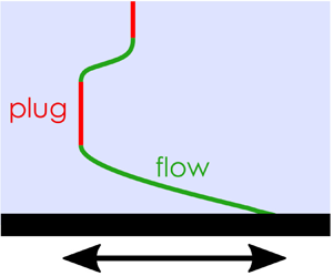
Figure 1. Schematic of the flow problem and example velocity profiles for (a) Newtonian fluid, (b) Bingham material with low-frequency plate oscillations relative to the time scale for momentum diffusion, and (c) Bingham material with higher-frequency oscillations.
To non-dimensionalise the system, the  $y$-coordinate is scaled with $H$, time with $1/\omega$, and shear stress with $\rho H \omega U_0$, giving
 \begin{equation} \hat{y}=\frac{y}{H}, \quad \hat{t} = \omega t, \quad \hat{\tau} = \frac{\tau}{\rho H \omega U_0}, \quad \hat{u} = \frac{u}{U_0}, \end{equation}
where the dimensionless variables are indicated with hatted symbols. This non-dimensionalisation differs to that of Balmforth et al. (Reference Balmforth, Forterre and Pouliquen2009), in that the  $y$-coordinate is scaled with the layer height $H$ here, producing different (but equivalent) forms of the dimensionless groups. The scaling used here produces a dimensionless layer height of unity, which facilitates comparison of the various flow regimes.
Omitting the hats for simplicity, the dimensionless system becomes
 \begin{equation} \frac{\partial u}{\partial t} = \frac{\partial \tau}{\partial y}, \end{equation}
with the constitutive law
 \begin{gather} \frac{\partial u}{\partial y} = 0, \quad \text{for} \ |\tau| \leq B, \end{gather}
 \begin{gather}\tau= \frac{1}{\alpha}\,\frac{\partial u}{\partial y} + B \operatorname{sgn} \left( \frac{\partial u}{\partial y} \right), \quad \text{for} \ |\tau| > B, \end{gather}
where the respective Bingham number and oscillatory Reynolds number (or Stokes number) are
 \begin{equation} B=\frac{\tau_Y}{\rho H U_0 \omega}, \quad \alpha = \frac{\rho \omega H^2}{\mu}. \end{equation}
The Bingham number  $B$ specifies the ratio of the yield stress to the inertial stress generated in the layer, while the oscillatory Reynolds number $\alpha$ gives the time scale for momentum diffusion relative to the imposed time scale of the oscillating plate. Because $B$ is independent of the shear viscosity of the material, the criterion for flow does not depend on $\alpha$ and is simply $B<1$ (see § 3.1).
The dimensionless boundary and initial conditions (2.3a–c) are
 \begin{equation} u(0, t) = \cos t , \quad u(y, 0) = 0, \quad \tau(1, t) = 0. \end{equation}
The boundary condition at  $y=0$ can be recast in terms of the shear stress using (2.5):
 \begin{equation} \left.\frac{\partial \tau}{\partial y}\right\rvert_{y=0} = \left.\frac{\partial u}{\partial t}\right\rvert_{y=0}={-} \sin t. \end{equation}
The layer is partitioned into rigid and yielded regions (figure 1):
 \begin{gather} \frac{\partial u}{\partial y} = 0, \quad \text{for} \ |\tau| \leq B \quad (\text{rigid}) , \end{gather}
 \begin{gather}\frac{\partial u}{\partial t} =\frac{1}{\alpha}\,\frac{\partial^2 u}{\partial y^2}, \quad \text{for} \ |\tau|>B \quad (\text{yielded}). \end{gather}
The initial transient occurring immediately after start up at  $t=0$ is ignored, and the analysis focuses on the periodic dynamics of the layer. The time taken to reach this periodic state is analysed in Appendix A.
2.1. General numerical results
The governing equation (2.5), constitutive law (2.6), and initial and boundary conditions (2.8a–c), are solved numerically for the shear stress  $\tau$. A finite-difference numerical method is used, the details of which are given in the appendices of Balmforth et al. (Reference Balmforth, Forterre and Pouliquen2009) and Hinton et al. (Reference Hinton, Collis and Sader2022); for simplicity, this will henceforth be referred to as the ‘arbitrary- $B$ numerical solution’. The velocity field $u$ is then computed via the momentum equation (2.5). A wide range of parameter values, $\alpha$ and $B$, is studied, with simulations run for sufficiently large times to ensure that the last two computed periods repeat, i.e. periodic behaviour is reached. Results for this periodic motion are shown in figure 2, with the start of the last two periods shifted to the origin (by subtracting an integer multiple of $2 {\rm \pi}$). The curved black lines in figure 2 indicate the yield surfaces – which delineate regions of rigid and fluid-like behaviour – with the colours specifying the velocity field. Note that the layer remains rigid everywhere when $B\geq 1$; see § 3. Accordingly, this study focuses on $B<1$ where the Bingham material can yield.

Figure 2. Velocity field (colour scales) and yield surfaces (black lines) of the periodic flow for nine pairs  $(\alpha,B)$ obtained using the arbitrary- $B$ numerical solution. The yield surfaces separate rigid and yielded regions as labelled in (d); similar labelling of the other panels is implied.
Small values of  $\alpha$ correspond to fast momentum diffusion through the yielded material, relative to the imposed oscillation time scale, i.e. vorticity diffuses quickly from the plate. In this case, the velocity gradient is small in yielded regions and vanishes in rigid regions. The fraction of the layer that is rigid is approximately proportional to the Bingham number. For $B \ll 1$, almost the entire layer yields except in a thin region near its free surface; see figure 2(g).
For large  $\alpha$, momentum diffusion is slow relative to the plate oscillation, and the shear stress decays rapidly away from the plate; see figures 2(c,f,i). Hence the yield surface is generally closer to the plate at higher values of $\alpha$. If $B$ is not small (see e.g. figure 2c), then the yielded region is very thin and the velocity at the free surface can be significant. This is because the layer is almost entirely rigid, through which momentum is transferred instantaneously. In the regime of large $\alpha$ and small $B$, multiple rigid regions can exist simultaneously in the material; see figure 2(i). The velocity field decays rapidly within the yielded region near the plate, and there is little momentum transfer to the free surface.
The detailed flow physics of these various regimes is explored in §§ 3 and 4.
3. Topology of the yield surfaces
In this section, we first determine the parameter values for which the layer yields at some point during its periodic motion (§ 3.1). In cases where the material does yield, we derive four properties for the topology of the yield surfaces in § 3.2. This has implications for the velocity at the free surface of the layer, which is discussed in § 3.3.
3.1. Criterion for flow
When the yield stress is large relative to the stress generated by the imposed plate oscillation – corresponding to larger values of  $B$ – the material is rigid throughout the layer. Consequently, the material velocity $u$ is independent of $y$, and differentiating (2.5) furnishes
 \begin{equation} \frac{\partial^2 \tau_R}{\partial y^2} = 0, \end{equation}
where the subscript  $R$ henceforth refers to the rigid region. The boundary conditions in (2.8a–c) and (2.9) then give
 \begin{equation} \tau_R=(1-y) \sin t. \end{equation}
This direct calculation of the stress within the rigid region is enabled by the unidirectional nature of the motion; the only non-zero component of the stress tensor is the shear stress. Note that gravity acting perpendicular to the plate would not alter the shear stress or velocity field within the layer. Because the material is rigid provided that  $|\tau |\le B$, as per (2.6), it follows from (3.2) that the material cannot yield if $B \ge 1$, i.e.
 \begin{equation} B < 1 \end{equation}
is required for flow to occur. This simple criterion is due to use of an inertial scale for the Bingham number in (2.7a,b), as mentioned above.
3.2. Key properties of the yield surfaces
Henceforth, we focus on the regime  $B <1$ in which at least some of the layer yields during parts of the motion. This implies the existence of yield surfaces, whose general behaviour is the focus of this section. Even when $B<1$, there can still be times when the layer is entirely rigid – which always gives the stress distribution in (3.2), being maximal at the plate surface $y=0$. As time evolves, these entirely rigid regions first yield when the magnitude of the stress matches the Bingham number at the plate, which from (3.2) gives
 \begin{equation} |{\sin t}| = B. \end{equation}
These critical (yielding) times are defined by
 \begin{equation} t_y = \sin^{{-}1} B + n {\rm \pi}, \end{equation}
where  $n \in \mathbb {Z}$. At $t=t_y$, the velocity across the rigid layer follows from (2.8a–c) and (3.5):
 \begin{equation} u_R={\pm}\sqrt{1-B^2}. \end{equation}
 After these critical times, the layer partitions into rigid and yielded regions that are separated by yield surfaces; see the black lines in figure 2. Since the stress is continuous across the layer and vanishes at its free surface, the layer is always rigid near its free surface. We denote the yield surface that is closest to the free surface by  $y=Y_1(t)$. From (3.1), it follows that the stress in the rigid region adjacent to the free surface ( $Y_1 < y \le 1$) is always given by
 \begin{equation} \tau_R = B \operatorname{sgn} \left(\frac{\partial u}{\partial y} \right) \left(\frac{1-y}{1-Y_1} \right). \end{equation}
 Acceleration of the yielded material at  $y=Y_1(t)$ is derived by integrating the momentum equation (2.5) over the uppermost rigid material (Sekimoto Reference Sekimoto1993; Balmforth et al. Reference Balmforth, Forterre and Pouliquen2009):
 \begin{equation} \frac{\partial u}{\partial t} = \frac{\partial u_R}{\partial t} ={-} \frac{B \operatorname{sgn} \! \left(\dfrac{\partial u}{\partial y} \right)}{1-Y_1}, \quad \text{at} \ y=Y_1(t). \end{equation}
The velocity gradient  $\partial u/ \partial y$ is continuous throughout the layer since the stress and the constitutive law (2.6) are continuous. Equation (2.10a) then establishes that the velocity gradient of the yielded material at the yield surface vanishes, i.e.
 \begin{equation} \frac{\partial u}{\partial y} =0, \quad \text{at} \ y=Y_1(t). \end{equation}
 There can be multiple rigid and yielded regions (see e.g. figure 2h), and we label the yield surfaces by  $y=Y_i(t)$ for $i=1,2,\dots,N$, where $Y_1(t)>Y_2(t)>\ldots >Y_N(t)$. In § 4, we determine criteria for which there can be an arbitrarily larger number $N$ of yield surfaces. Each yield surface emanates from the plate when the material changes its state from rigid to yielded, or vice versa; see figure 3. Consequently, the uppermost yield surface $Y_1(t)$ is always the ‘oldest’. The yield surfaces can terminate either by colliding with the plate or by colliding with each other; they cannot reach the free surface of the layer, as the stress here must vanish. Plate collision is possible only for the lowest yield surface. On each yield surface, the stress is constant and equal to either $+B$ or $-B$.
$-B$.

Figure 3. Schematic illustration showing qualitative behaviour of the yield surfaces; not calculated using the arbitrary- $B$ numerical solution. (a) Case of at most one yield surface. (b) Case of two or more yield surfaces co-existing, an example of which is indicated by the vertical red dashed line. On the boundary of the first yielded region, the propagation direction of the yield surfaces is indicated by arrows, emanations by red circles, and collisions by open red squares.
Next, we describe and explain four key properties of the yield surfaces. The reader is also referred to figure 2.
3.2.1. Property 1
If the material ever yields, then there are exactly four intersections of yield surfaces with the plate in any  $2 {\rm \pi}\ $ time period.
In any  $2 {\rm \pi}$ time period, the magnitude of the stress at the plate must exceed $B\ (<1)$ at some time for the material to generate a yield surface (whose state of stress is $\pm B$). By symmetry, the stress at the plate must be algebraically lower than $-B$ at some time, and greater than $+B$ at another time. Continuity of stress at the plate as time evolves implies that it crosses $+B$ twice and $-B$ twice, which gives four intersections of the yield surface with the plate. A consequence is that the stress at the yield surfaces intersecting the plate follows a periodic sequence of values as a function of time, $\{+B, +B, -B, -B\}$; see figure 3.
3.2.2. Property 2
Any yield surface emanating from the plate, upon the material changing from a yielded to a rigid state at that position, cannot collide with the plate.
In other words, when a yield surface emanates from the plate, there are two scenarios: (a) the yield surface collides with the plate (e.g. figures 2a and 3a), or (b) a second yield surface emanates from the plate, encapsulating a parcel of yielded material that moves through the material (e.g. figures 2h and 3b). This parcel cannot collide with any other parcel of yielded material and must vanish within the layer before reaching the free surface. To arrive at this conclusion, we make the following observations.
(i) Yield surfaces can collide with each other only if they have the same state of stress – otherwise, the stress would jump discontinuously within the layer, which is unphysical.
(ii) Because the motion is periodic, with yield surfaces having the sequential stress states defined in Property 1, it follows that the pairs of yield surfaces emanating from the plate with identical stress states must collide, as illustrated in figure 3. Otherwise, there would be a growing number of yield surfaces from one period to the next, violating periodicity. Collision can occur in subsequent periods; see § 4.2;
(iii) The material between two yield surfaces, at any time, is entirely rigid if and only if the stresses on those yield surfaces are of opposite sign, i.e. they have differing states of stress. Otherwise, additional yield surfaces separating yielded and rigid regions must exist between the two original yield surfaces. This is because the stress must vary continuously from one yield surface to another, and in any rigid region, the stress varies linearly with position; see (3.1).
(iv) For the same reason, a material between two yield surfaces is entirely yielded if and only if the stresses on those yield surfaces are identical, i.e. they have the same sign.
(v) It then follows from (i)–(iv) that a yield surface emanating from the plate due to a rigid-to-yielded transition of the material must collide with any second yield surface (of identical stress state) that emanates due to a yielded-to-rigid transition; see figure 3(b).
Consequently, the yield surface emanating from the plate due to a yielded-to-rigid transition of the material cannot collide with the plate, establishing Property 2.
It follows that every rigid region must eventually incorporate the free surface; it cannot terminate within the layer. Any rigid region cannot be terminated by collision of its two bounding yield surfaces; see (i) above.
3.2.3. Property 3
Two or more yield surfaces co-exist at any time during the motion if and only if the layer never becomes entirely rigid.
Suppose that two yield surfaces co-exist within the layer at some time. There must be an (upper) rigid region adjacent to the free surface, whose stress distribution is
 \begin{equation} \tau_R ={\pm} B\,\frac{1-y}{1-Y_1}, \end{equation}
where  $y=Y_1$ is the position of the upper yield surface, below which yielded material must reside (by definition). It then follows that the second (lower) yield surface at $y = Y_2$ has the same state of stress (see (iv) above) and resides next to the plate. That is, there is a second rigid region adjacent to the plate, whose stress distribution is
 \begin{equation} \tau_R = \left(Y_2 -y\right) \sin t \pm B. \end{equation}
 Because these two yield surfaces have the same state of stress, they must eventually collide within the layer; see (ii) above and figure 3(b). At collision, the material acceleration  $\partial u/\partial t$ must be continuous, hence $\partial \tau /\partial y$ is continuous, via (2.5). It then follows from (3.10) and (3.11) that the collision time $t=t_c$ (where $Y_1 = Y_2$) is given by
 \begin{equation} |{\sin t_c}| = \frac{B}{1-Y_1} > B, \end{equation}
because  $Y_1 > 0$ from Property 2. If no other yield surfaces exist at this collision time, then the layer will be entirely rigid and the stress magnitude will exceed $B$ in the region $0< y < Y_1(t_c)$, i.e. a contradiction. Thus, a new yield surface must emanate from the plate at or before the collision of the two yield surfaces; see figure 3(b).
In other words, when two yield surfaces co-exist, the layer is never entirely rigid; this finding also applies to three or more co-existing yield surfaces. Conversely, for the layer to never be entirely rigid over a  $2 {\rm \pi}$ time period, there must be at least two yield surfaces at some time. This is because a single yield surface would collide with the plate, leaving the layer entirely rigid at some times.
An obvious consequence is that there is at most one yield surface if and only if the layer becomes entirely rigid at some time in each  $2{\rm \pi}$ time period; see figure 3(a).
3.2.4. Property 4
If the Bingham number exceeds  $B_{critical} = \textit {0.5370}$, then there is at most one yield surface.
Suppose that the layer is entirely rigid and then yields at some time  $t=t_y$. A single yield surface must emanate from the plate. From (3.8), acceleration of the rigid region adjacent to the free surface then satisfies
 \begin{equation} \left| \frac{\partial u_R}{\partial t} \right| = \frac{B}{1-Y_1} \geq B, \end{equation}
which gives  $\partial u_R/\partial t \leq -B$ for $u>0$, and $\partial u_R/\partial t \geq +B$ for $u<0$. Since the entire layer has velocity $u=\pm \sqrt {1-B^2}$ at $t=t_y$ (see (3.6)), it then follows that the yield surface velocity satisfies
 \begin{equation} u_R \leq \sqrt{1-B^2} - B(t-t_y) \quad \text{or} \quad u_R \geq{-}\sqrt{1-B^2} + B(t-t_y). \end{equation}
These bounds are shown as a green dashed line in figures 4(a,b). If the yield surface subsequently collides with the plate, then the rigid region will match the plate velocity at that collision time  $t=t_c$, i.e. $u=\cos t_c$. From (3.14), it follows that the latest the collision time can occur (i.e. an upper bound) is given by
 \begin{equation} \cos t_c = \sqrt{1-B^2} - B(t_c-t_y). \end{equation}
Subsequently, the entire layer becomes rigid and then yields again at  $t=t_y+{\rm \pi}$, by periodicity. If this second yield time occurs after the latest collision time, defined by (3.15), then only one yield surface can arise. Substituting $t_c=t_y+{\rm \pi}$ into (3.15), we obtain the condition
 \begin{equation} B \geq B_{critical} = \left( 1+ \frac{{\rm \pi}^2}{4} \right)^{-{1}/{2}} \approx 0.5370, \end{equation}
which is sufficient to ensure that only one yield surface can exist, e.g. figures 2(a–c). This sufficient condition is satisfied in figure 4. Collision with the plate is seen to always occur prior to the second yield time,  $t=t_y+{\rm \pi}$ (shown as a vertical dashed line), as required. Because (3.16) is derived using an upper bound for the collision time, it follows that only one yield surface may occur for smaller values of $B$, e.g. figure 2(d).

Figure 4. Free-surface velocity  $u = u_R$ (solid coloured lines), and the plate velocity $u=\cos t$ (solid black line) for (a) $B=0.6$, and (b) $B=0.8$, for two values of the oscillatory Reynolds number $\alpha$. The straight green dashed line gives the fastest (or slowest) possible motion of the rigid region, as per (3.14). (c,d) Corresponding plots of the yield surface. The vertical dashed lines are at the yield times $t_y=\sin ^{-1} B$ and $t=t_y +{\rm \pi}$, from (3.5).
3.3. Condition for a maximum free-surface speed of unity
The above findings have implications for the free-surface speed. If the layer is never entirely rigid, then the free surface never moves in concert with the plate. Hence if there are two or more yield surfaces – or equivalently, the layer is never entirely rigid (as per Property 3) – then viscous effects damp the motion and the maximum free-surface speed must be strictly less than unity.
However, existence of an entirely rigid layer is not sufficient to ensure that the maximum magnitude of the free-surface speed is unity, because the layer may not be entirely rigid when the plate speed is unity. Thus ensuring magnitude unity of the maximum free-surface speed requires a condition stronger than (3.16), which we derive below.
We consider a single yield surface, otherwise the maximum free-surface speed cannot be unity. The resulting single rigid region incorporates intrinsically the free surface. The material yields at time  $t_y=\sin ^{-1} B + n {\rm \pi}$, as per (3.5). Subsequently, the velocity of the single rigid region (and hence the free surface) is bounded by (3.14), shown as dashed green lines in figure 4. For simplicity, we examine the dynamics of the layer starting from $t=0$ (i.e. $n=0$ in (3.5)), while noting that the derived condition in (3.19) holds for all periods of motion. For the free surface to attain velocity $u=\pm 1$, the yield surface must collide with the plate before $t= {\rm \pi}$. This is because the plate velocity is $u=-1$ at $t= {\rm \pi}$. If the collision occurs later, then the entirely rigid layer (and the plate) moves slower than $|u|=1$. The velocity of the yield surface at $t={\rm \pi}$ is at most specified by (3.14), which, by using the result for the yield time $t_y$ in (3.5), gives
 \begin{equation} u_R |_{t={\rm \pi}} \leq \sqrt{1-B^2}- B ({\rm \pi} -\sin^{{-}1} B). \end{equation}
For collision with the plate to occur prior to  $t={\rm \pi}$, the rigid region velocity at $t={\rm \pi}$, $u_R |_{t={\rm \pi} }$, which decreases linearly in time, would be algebraically less than $-1$. Hence (3.17) establishes that the lowest value of $B = B_{unity}$ for this collision to occur is given by
 \begin{equation} \sqrt{1-B_{unity}^2} - B_{unity} \left({\rm \pi} -\sin^{{-}1} B_{unity}\right) ={-}1, \end{equation}
which implies that the maximum free-surface speed is unity if
 \begin{equation} B \geq B_{unity} = 0.7246. \end{equation}
As expected, this condition is stricter (higher value of  $B$) than ensuring that a single yield surface exists; see (3.16). Similar to (3.16), the condition (3.19) is sufficient but not necessary to ensure a maximum free-surface speed of unity. Results for $B=0.6\ (< B_{unity})$ are given in figures 4(a,c) and exhibit only one yield surface. Even so, collision can occur after $t={\rm \pi}$ (as for $\alpha =100$) for which the maximum free-surface speed is less than unity. In contrast, results for $B=0.8\ (>B_{unity})$ in figures 4(b,d) also display one yield surface, which collides with the plate prior to $t={\rm \pi}$ – so the maximum free-surface speed is unity for all values of $\alpha$.
3.4. Bounds for the stress, acceleration and uppermost yield surface
The magnitude of the plate acceleration is  $|{\sin t}|$, which is at most $1$. Because additional acceleration cannot be generated within the layer, the acceleration is everywhere bounded by
 \begin{equation} \left| \frac{\partial u}{\partial t} \right| \leq 1. \end{equation}
In other words, the acceleration attains its maximum and minimum at the plate. It follows from (2.5) that  $|\partial \tau /\partial y| \leq 1$. Hence the stress in the layer satisfies
 \begin{equation} |\tau| \leq 1-y. \end{equation}
The material in  $1-B < y < 1$ is always rigid, hence yield surfaces cannot enter this region. The uppermost yield surface touches $y=1-B$ in the limit $\alpha \to 0$; see § 4.1.
4. Asymptotic behaviour of the yield surfaces and velocity field
In this section, we analyse the different periodic regimes that occur in each region of the  $(\alpha,B)$ parameter space for $B<1$. We use asymptotic analysis to draw out the dominant physical processes in each regime.
We work through the parameter space of figure 2 in an anticlockwise fashion. We begin in § 4.1 with the low-frequency limit,  $\alpha \ll 1$. Our analysis proceeds to the case of low yield stress for which there are two sub-regimes in §§ 4.2 and 4.3. Finally, in § 4.4, we consider flows that occur at high oscillation frequencies, $\alpha \gg 1$. Peripheral details are relegated to appendices. Specifically, behaviour of a Newtonian layer ( $B=0$) is recalled in Appendix B. The case of a layer that is predominantly rigid and yields at the plate for just a short period of time during each oscillation cycle is discussed in Appendix C; this occurs when $B$ is just less than $1$. The detailed asymptotic behaviours immediately after emanation of a single yield surface, immediately prior to collision of a single yield surface with the plate, and immediately prior to collision of two yield surfaces, are given in §§ D.1 and D.2, and Appendix E, respectively.
4.1. Low-frequency regime
In the low-frequency (quasi-steady) limit,  $\alpha \to 0$, momentum diffusion across any yielded region is instantaneous, hence the evolution of each yield surface is symmetric in time; see figure 5. The velocity field $u$ in any yielded region is governed by (2.10b), which in the low-frequency limit becomes
 \begin{equation} \frac{\partial^2 u}{\partial y^2 }={O}(\alpha), \end{equation}
whilst in any rigid region, we have  $\partial u/\partial y=0$. Hence, throughout the layer, the velocity is
 \begin{equation} u=\cos t + {O}(\alpha), \end{equation}
i.e. the entire layer (both rigid and yielded regions) moves in concert with the oscillating plate. The boundary condition at the uppermost yield surface (3.8) then gives the leading-order evolution of its position:
 \begin{equation} {Y_1}=\max \left(0,1-\frac{B}{|{\sin t}|}\right) + {O}(\alpha). \end{equation}
The maximum-yield surface height is
 \begin{equation} Y_{max}=1-B + {O}(\alpha), \end{equation}
which occurs at  $t= (n+1/2){\rm \pi} + {O}(\alpha )$. Equation (4.4) is the maximum height of the uppermost yield surface for fixed $B$ and any $\alpha$; see § 3.4.

Figure 5. Yield surfaces for  $\alpha =0.05$ and three values of $B$. The arbitrary- $B$ numerical solution (black line) is compared to the asymptotic solution for small $\alpha$, (4.3) (red dashed line).
The asymptotic solution in (4.3) exhibits good agreement with the arbitrary- $B$ numerical solution for small $\alpha$; see figure 5.
4.2. Small yield stress: yield surface is asymptotically close to the free surface
For small Bingham numbers  $B \ll 1$, provided that the Stokes number $\alpha$ is not too large, the uppermost yield surface will periodically become close to the free surface, e.g. figures 2(g) and 8. The condition on $\alpha$ under which this occurs is provided in (4.11). Because $B$ is small and virtually the entire layer yields, the leading-order velocity $u$ in the small- $B$ limit is given by the Newtonian solution, i.e. $u=u_N(y,t) + {O}(B)$, where $u_N(y,t)$ is given in (B1).
4.2.1. Dynamics of the uppermost yield surface
Discussion in the preceding paragraph motivates the following asymptotic expansion for the uppermost yield surface:
 \begin{equation} Y_1 = 1-B \tilde{Y} +o(B) , \quad u =u_N+Bu_1 +o(B) . \end{equation}
The boundary condition at the yield surface (3.8) furnishes
 \begin{equation} \tilde{Y} = \Bigg\rvert \frac{\partial u_N}{\partial t}\Big\rvert_{y=1} \Bigg\rvert ^{{-}1}. \end{equation}
Using the Newtonian solution in (B1), and the closed form of its acceleration at the free surface (B3), then gives
 \begin{equation} Y_1 = 1- \frac{B}{|{\sin (t-\sigma)}|} \sqrt{\frac{\cos \sqrt{2 \alpha} + \cosh \sqrt{2 \alpha}}{2}} +o(B) , \end{equation}
where  $\sigma$ is the phase shift in the yield surface maximum from the quasi-steady small- $\alpha$ behaviour described in § 4.1; see also (4.10) below. It is given by
 \begin{equation} \tan \sigma = \tanh \sqrt{\frac{\alpha}{2}} \tan \sqrt{\frac{\alpha}{2}}. \end{equation}
Equations (4.5a,b) and (4.7) establish that the maximum-yield surface height  $Y_{max}$ is
 \begin{equation} Y_{max}=1- B \sqrt{ \frac{\cos \sqrt{2 \alpha} + \cosh \sqrt{2 \alpha}}{2}} +o(B) , \end{equation}
which occurs at time
 \begin{equation} t = t_{max}=\left(n+\tfrac{1}{2}\right) {\rm \pi}+ \sigma +o(1). \end{equation}
The prediction for the maximum height of the yield surface (4.9) is compared to the arbitrary- $B$ numerical solution in figure 6.


Figure 7 shows that the phase shift  $\sigma$ is an increasing function of $\alpha$; see (4.7) and figure 8. Indeed, $\sigma \to 0$ in the small-frequency limit ( $\alpha \to 0$), where (4.3) is recovered.

Figure 7. Relationship between the phase shift  $\sigma$ of the uppermost yield surface and the oscillation frequency $\alpha$, according to (4.8).

Figure 8. Yield surface for small Bingham number,  $B=0.1$. (a–c) Smaller frequency values. The arbitrary- $B$ numerical solution (black line) is compared to the asymptotic solution (4.7) (red dashed line). (d–f) Larger frequency values. The yield surface does not come close to the free surface, and (4.3) is not valid (its solution is not shown). The red circles represent the times from (4.14) when yield surfaces are predicted to emanate from the plate.
Figure 8 shows a comparison between (4.7) (red dashed lines) and the arbitrary- $B$ numerical solution (black lines). By construction, the asymptotic expansion is expected to describe the behaviour accurately only at times when the yield surface is near the free surface. It is evident from (4.7) and (4.9) that proximity of the yield surface to the free surface requires small to moderate values of $\alpha$, which is borne out in figure 8(a–c).
The second term on the right-hand side of (4.7) grows with increasing  $\alpha$, i.e. the yield surface moves away from the free surface. It then follows from that second term that the yield surface will come close to the free surface if
 \begin{equation} B \ll \exp\left(-\sqrt{\frac{\alpha}{2}}\right), \end{equation}
in which case the asymptotic expansion in (4.7) remains valid. Equation (4.11) is the required condition for the present low yield stress and low-to-moderate frequency regime. For example, figure 9(a) shows numerical results for  $B=0.001$ and $\alpha =25$ where the yield surface comes close to the free surface; these parameters satisfy (4.11), as required.


4.2.2. Shear stress at the plate
The leading-order velocity gradient at the plate in this small yield stress limit is obtained by differentiating the Newtonian solution in (B1), given in closed form as (B5). The shear stress at the plate in the yielded region then follows from (2.6), giving
 \begin{equation} \tau |_{y=0} ={\pm}\left( B+ \frac{\sqrt{\alpha \sin^2 \sqrt{2 \alpha}+ \alpha \sinh^2 \sqrt{2\alpha} }}{\cos \sqrt{2 \alpha} +\cosh \sqrt{2 \alpha}}\,|{\sin(t-\gamma)} |\right) + o(B), \end{equation}
where  $\gamma$ is the phase shift of the yield surface emanation or collision time from the quasi-steady small- $\alpha$ behaviour described in § 4.1. It is given by
 \begin{equation} \tan \gamma = \frac{\sinh\sqrt{2\alpha} - \sin \sqrt{2\alpha}}{\sinh\sqrt{2\alpha} + \sin \sqrt{2\alpha}}. \end{equation}
 Figure 10 shows that  $\gamma$ is a non-monotonic function of $\alpha$ that asymptotes to $\gamma = {\rm \pi}/4$ as $\alpha \to \infty$; the maximum value $\gamma \approx 0.8133\ (>{\rm \pi} /4)$ occurs at $\alpha = 25 {\rm \pi}^2/32 \approx 7.7106$. Equation (4.12) shows that the magnitude of the stress at the plate surface equals the yield stress when $|{\sin (t-\gamma )}|=0$, at which time, $t = t_c$, a yield surface emanates from or collides with the plate, where
 \begin{equation} t_c= n {\rm \pi}+ \gamma + o(1), \end{equation}
with  $n \in \mathbb {Z}$. This asymptotic solution for $t_c$ in the small- $B$ limit is shown in figures 8 and 9 by red circles. It displays good agreement with the arbitrary- $B$ numerical solution for the time at which a yield surface (associated with a yielded to rigid transition) emanates from the plate. In the limit as $B \to 0$, the time interval over which rigid material exists at the plate is very small, and the time $t_c$ corresponds to emanation of two yield surfaces (almost simultaneously) that bound the rigid material; see figure 9. When $B$ is not so small, rigid regions exist over longer periods at the plate surface, i.e. the two yield surfaces are further separated in space and time.

Figure 10. Relationship between the phase shift  $\gamma$ of the yield surface collision/emanation at the plate and the oscillation frequency $\alpha$, according to (4.13).
We have introduced two phase shifts: (i)  $\sigma$ is the shift of the yield surface peak from the small- $\alpha$ behaviour, which grows unboundedly with $\alpha$ (see figure 7); and (ii) $\gamma$ is the phase shift of the emanation time from the plate and is bounded (see figure 10). Combination of these two shifts suggests that yielded parcels of material can exist for increasingly longer times at larger $\alpha$, provided that $B$ is sufficiently small (e.g. figure 9b).
4.2.3. Existence of two or more yield surfaces
The analysis in §§ 4.2.1–4.2.2 can be deployed to predict when two or more yield surfaces can occur. An entirely rigid layer yields at times
 \begin{equation} t= \sin^{{-}1} B + n{\rm \pi}, \end{equation}
as per (3.5). The collision/emanation time in (4.14) must occur whilst the layer is entirely rigid. Otherwise, a second yield surface would emanate, and by Property 3 (§ 3.2.3), the layer would never be entirely rigid, leading to a contradiction. Hence from (4.14) and (4.15), the following conditions arise (for small  $B$):
$B$):
 \begin{gather} \text{at most one yield surface exists if and only if } \sin^{{-}1} B > \gamma; \end{gather}
 \begin{gather}\text{two or more yield surfaces exist if and only if } \sin^{{-}1} B < \gamma. \end{gather}
The latter condition becomes
 \begin{equation} B < \frac{\sinh \sqrt{2 \alpha}-\sin \sqrt{2 \alpha}}{\sqrt{2 \sinh^2 \sqrt{2 \alpha} +2 \sin^2 \sqrt{2 \alpha}}}. \end{equation}
Equation (4.17) is relevant to small  $\alpha$ because this analysis requires $B \ll 1$; see figures 8(a,b). For $\alpha \ll 1$, this gives the required necessary and sufficient condition for existence of two or more yield surfaces:
 \begin{equation} B < \frac{\alpha}{3} + o(\alpha). \end{equation}
 For larger values of  $\alpha$, the condition in (3.16) becomes necessary and sufficient for distinguishing the existence of a single yield surface from multiple yield surfaces; see § 4.4. We can combine (3.16) and (4.18) to obtain the following uniformly valid approximate formula that delineates the existence of one or multiple yield surfaces:
 \begin{equation} B\approx\frac{\alpha}{\sqrt{9+\left(1+\displaystyle \frac{{\rm \pi}^2}{4}\right) \alpha^2}}. \end{equation}
Figure 11 shows that (4.19) provides an approximate yet accurate solution to the problem.

Figure 11. Phase diagram showing the number of yield surfaces as a function of the oscillation frequency  $\alpha$ and Bingham number $B$, calculated using the arbitrary- $B$ numerical solution (black line) and the approximation in (4.19) (red dot-dashed line).
4.2.4. High oscillation frequency
For high oscillation frequency, i.e.  $\alpha \gg 1$, where the yield surface comes close to the free surface, i.e. $B\ll \exp (-\sqrt {\alpha /2})\ll 1$ as per (4.11), the analysis above applies with large phase shift, $\sigma \approx \sqrt {\alpha /2}$, as per (4.8). The high oscillation frequency, relative to momentum diffusion, ensures that the free-surface velocity is small. Away from the free surface, the velocity field in the yielded material is given by that of a semi-infinite layer of Newtonian fluid, (B7). Therefore, the shear stress in this layer is
 \begin{equation} \tau={\pm} B + \frac{1}{\sqrt\alpha} \sin \left(t - y \sqrt{\frac{\alpha}{2}} - \frac{\rm \pi}{4}\right) \exp \bigg({-}y \sqrt{\frac{\alpha}{2}}\, \bigg) + o \bigg( \sqrt{\frac{1}{\alpha}}\, \bigg), \end{equation}
where the first term on the right-hand side is of identical sign to the second term, by definition. Consequently, the stress changes sign along yield surfaces defined by straight lines in  $(y,t)$ space:
 \begin{equation} Y(t) = \left(t- {\rm \pi}\left[n + \frac{1}{4} \right] \right) \sqrt{\frac{2}{\alpha}} + o \bigg( \sqrt{\frac{1}{\alpha}}\,\bigg), \end{equation}
where  $n \in \mathbb {Z}$. In dimensional terms, the yield surface and disturbances propagate through the layer with speed $\sqrt {2 \omega \mu /\rho }$, as in the classical Stokes layer. Equation (4.21) is shown as red lines in figure 9. Increasing the oscillation frequency $\alpha$ hinders momentum diffusion, with the thin rigid regions taking longer to reach the free surface. In this high-frequency limit, (4.21) gives an identical result to (4.14) for the time at which yield surfaces emanate from the plate, i.e. $\gamma \to {\rm \pi}/4$ as $\alpha \to \infty$. The shift in the time for the yield surface to attain its maximum is $\sigma \approx \sqrt {\alpha /2} \gg 1$.
It follows from (4.21) that three successive rigid regions co-exist in the layer when  $\alpha > 2 {\rm \pi}^2$, and a total of $N$ distinct rigid regions co-exist for
 \begin{equation} \alpha > 2(N-2)^2 {\rm \pi}^2. \end{equation}
That is, the number of distinct rigid regions that co-exist is
 \begin{equation} N = \left\lfloor 2+ \frac{1}{\rm \pi} \sqrt{\frac{\alpha}{2}} \right\rfloor, \end{equation}
for  $B\ll \exp (-\sqrt {\alpha /2}) \ll 1$. Hence in this regime, any number of yield surfaces can co-exist simultaneously for sufficiently large oscillation frequency $\alpha$. The maximum free-surface speed in this regime follows from (B7):
 \begin{equation} \max\left| u |_{y=1} \right| =\exp \left(-\sqrt{\frac{\alpha}{2}}\right). \end{equation}
4.3. Small yield stress: yield surface does not come close to the free surface
In the present subsection, we consider the regime of small  $B$ but with larger values of $\alpha$ such that the uppermost yield surface does not come close to the free surface. We focus on the regime
 \begin{equation} \exp \left(-\sqrt{\frac{\alpha}{2}}\right) \ll B \ll 1. \end{equation}
Since  $\alpha$ is large and $B \ll 1$, the velocity field between the plate and the uppermost yield surface is well-approximated by that of a semi-infinite layer of Newtonian fluid, given by (B7). Yielding is confined to this thin region near the oscillating plate. It is worth noting that a very thick layer (i.e. large $H$) corresponds to $B \sim 1/\sqrt {\alpha } \ll 1$ (see (2.7a,b)), which lies in the regime given by (4.25).
4.3.1. Uppermost yield surface
The boundary condition at the uppermost yield surface in (3.8), then becomes
 \begin{equation} \left|\sin\bigg( t -\frac{\hat{Y}_1}{\sqrt{2}}\bigg)\right| \exp\bigg(-\frac{\hat{Y}_1}{\sqrt{2}}\bigg)=\frac{B}{1-\hat{Y}_1/\sqrt{\alpha}} = B + {O}\! \left(\frac{1}{\sqrt{\alpha}}\right), \end{equation}
where
 \begin{equation} \hat{Y}_1 = \sqrt{\alpha}\,Y_1. \end{equation}
The implicit solution to (4.26) is
 \begin{equation} t =n{\rm \pi}+ \frac{\hat{Y}_1}{\sqrt{2}} \pm \sin^{{-}1} \left[ B \exp\bigg(\frac{\hat{Y}_1}{\sqrt{2}}\bigg) \right] + {O} \left(\frac{1}{\sqrt{\alpha}}\right), \end{equation}
where  $n \in \mathbb {Z}$, and the $\pm$ sign is chosen such that $\hat {Y}_1$ is the uppermost yield surface. Equation (4.28) is shown as the blue dot-dashed line in figure 12, where it is compared to the arbitrary- $B$ numerical solution; the grey dotted vertical lines indicate the transition from one uppermost yield surface to another. The maximum height of the yield surface and the time at which it is attained are given by
 \begin{equation} Y_{max}={-} \sqrt\frac{2}{\alpha} \log{B} + o \left( \frac{\log B}{\sqrt{\alpha}} \right), \quad t_{max}=\left(n+\frac{1}{2}\right){\rm \pi} - \log B + o ( 1 ). \end{equation}
Note that  $t_{max}$ depends only on $B$ and not on $\alpha$, consistent with the arbitrary- $B$ numerical solution in figures 8(d–f). Equations (4.29a,b) are compared to the arbitrary- $B$ numerical solution in figure 6. The maximum-yield surface height, $Y_{max}$, is close to the plate provided that $\exp (-\sqrt {\alpha /2}) \ll B < 1$, as expected. The time $t_{max}$ is also the termination time of the uppermost yield surface. Hence if
 \begin{equation} \log B <{-} 2 {\rm \pi}, \end{equation}
then at least three distinct rigid regions can co-exist. Any number  $N$ of distinct rigid regions co-exist for
 \begin{equation} \log B <{-} (N-1) {\rm \pi}\end{equation}
provided that  $\exp (-\sqrt {\alpha /2}) \ll B < 1$. Consequently, we can combine (4.31) in the present regime with (4.23), which holds when the yield surface is close to the free surface, to obtain
 \begin{equation} N= \left\lfloor 1- \frac{\log B}{\rm \pi} \right\rfloor, \end{equation}
which is valid provided that  $\alpha \gg 1$, independently of whether the yield surface comes close to the free surface.


We have described the dynamics of the uppermost yield surface,  $Y_1(t)$, and now proceed to describe the next two yield surfaces (when they exist).
4.3.2. Second yield surface
The second yield surface,  $Y_2(t)$, emanates from the plate when the material there becomes rigid. Whilst the material at the plate is rigid, the velocity at $y=Y_2(t)$ is equal to the velocity of the plate. In this high- $\alpha$ limit, the velocity at this yield surface is also equal to that of a semi-infinite Newtonian layer, which, using (B7), gives
 \begin{equation} \cos t = \cos \left(t-\sqrt{\frac{\alpha}{2}}\,Y_2\right)\exp\left({-}Y_2\sqrt{\frac{\alpha}{2}}\right) + {O}\! \left(\frac{1}{\alpha}\right). \end{equation}
Taking the limit  $Y_2 \to 0$ gives the emanation time of this second yield surface (see e.g. figure 12) as
 \begin{equation} t_2 = \left(n+ \tfrac{1}{4}\right) {\rm \pi}+ o(1). \end{equation}
This is of the same form as (4.14) because these emanation times are controlled by the semi-infinite Newtonian solution, as  $\alpha \to \infty$. The solution to (4.33) is
 \begin{equation} t= n {\rm \pi}+ \tan^{{-}1} \left( \frac{\exp \left(\displaystyle \frac{\hat{Y}_2}{\sqrt{2}}\right) -\cos \left(\displaystyle \frac{\hat{Y}_2}{\sqrt{2}}\right)}{\sin\left(\displaystyle \frac{\hat{Y}_2}{\sqrt{2}}\right)} \right) + o (1), \end{equation}
where  $\hat {Y}_2=Y_2 \sqrt {\alpha }$. Equation (4.35) gives the position of the second yield surface, $Y_2(t)$, and is shown as the red dashed line in figure 12.
4.3.3. Third yield surface
The shear stress in the rigid region between the second yield surface  $Y_2(t)$ and the plate is
 \begin{equation} \tau = (Y_2-y) \sin t \pm B. \end{equation}
As time evolves, the shear stress at the plate surface  $y=0$ in this rigid region starts at $\tau |_{y=0} = \pm B$, and subsequently decays to zero, before switching sign and approaching the yield stress of opposite sign, i.e. $\tau |_{y=0} = \mp B$. From (4.36), it then follows that a third yield surface emanates from the plate at time $t = t_3$ satisfying
 \begin{equation} Y_2(t_3) = \frac{2B}{|{\sin t_3}|}. \end{equation}
 Equation (4.33) shows that  $Y_2={O}(1/\sqrt {\alpha })$, which together with (4.37) establishes that the third yield surface cannot arise when
 \begin{equation} B \gg \frac{1}{\sqrt{\alpha}}. \end{equation}
Conversely, if  $B \ll 1/\sqrt {\alpha }$, then (4.37) implies that emanation of the third yield surface occurs when $\hat {Y}_2=Y_2 \sqrt {\alpha } \ll 1$. Small $\hat {Y}_2$ occurs very shortly after the emanation of $Y_2$ (see (4.34) and (4.35)), so $t_3 \approx t_2$. That is, the rigid region between the second and third yield surfaces is small.
Because the new yielded region associated with  $Y_3(t)$ diffuses from the plate and is unhindered by the free surface (due to high $\alpha$), this yield surface follows a trajectory identical to the particle paths of a semi-infinite Newtonian layer, i.e.
 \begin{equation} Y_3(t) = \sqrt{\frac{2}{\alpha}}\,(t-t_3). \end{equation}
Equation (4.39) is shown as the green dotted line in figure 12. When  $Y_2$ and $Y_1$ collide, $Y_3$ becomes the new $Y_1$, and its evolution changes qualitatively; this transition is manifested in figure 12 as cusps in the arbitrary- $B$ numerical solution.
When there are more than three yield surfaces, pairs of yield surfaces emanate at times given by (4.34) and propagate from the plate with speed  $\sqrt {2/\alpha }$. This is analogous to the behaviour in figure 9(b) for termination of the first and second yield surfaces, except that these subsequent yield surfaces terminate near the plate.
4.4. Moderate-to-large yield stress: yield surface not close to the free surface
Next, we consider the high-frequency limit,  $\alpha \gg 1$, where the yield surface does not come close to the free surface, i.e. $Y \ll 1$. This is imposed together with the condition that the Bingham number $B$ is of order $1$, and $B<1$. The boundary condition (3.8) at the uppermost yield surface then becomes
 \begin{equation} \frac{\partial u_R}{\partial t} ={\pm} B + o(1). \end{equation}
Hence the inequality in (3.13) becomes an equality, and the condition for at most one yield surface to exist, (3.16), becomes necessary and sufficient. That is, there is at most one yield surface for  $B \ge B_{critical} = 0.5370$, and there must be a time when there are two (or more) yield surfaces for $B<0.5370$ in this high- $\alpha$ limit. This feature is demonstrated in figure 13(a).

Figure 13. (a) Yield surfaces for  $\alpha =200$ and four values of $B$ (only one yield surface in the time evolution is shown). (b) Yield surfaces for $B=0.4$ and $\alpha =50, 100, 200, 400$, rescaled to demonstrate that $Y \sim 1/\sqrt {\alpha }$ for $\alpha \gg 1$.
4.4.1. Only one yield surface exists ( $B>0.5370$)

The form of the governing equation for the yielded region, (2.10b), suggests the rescaling
 \begin{equation} \hat{y} = \sqrt \alpha\,y. \end{equation}
Equation (2.10b) and its associated boundary conditions for the yielded region, which make use of (4.40), then become
 \begin{equation} \frac{\partial u}{\partial t} = \frac{\partial^2 u}{\partial \hat{y}^2}, \end{equation}
with boundary conditions
 \begin{equation} \left .\frac{\partial u}{\partial t} \right|_{\hat{y}=\hat{Y}_1} ={\pm} B + o(1), \quad \left . \frac{\partial u}{\partial \hat{y}} \right|_{\hat{y}=\hat{Y}_1} =0, \end{equation}
where  $\hat {Y}_1 = \sqrt \alpha \,Y_1$, and
 \begin{equation} u |_{\hat{y}=0} =\cos t . \end{equation}
 Equations (4.42)–(4.44) are independent of  $\alpha$, which is consistent with the arbitrary- $B$ numerical solution in figure 13(b). These equations constitute a Stefan problem with an unknown free boundary $Y_1(t)$, which can be solved numerically for any value of $B$; see Hinton et al. (Reference Hinton, Collis and Sader2022).
The maximum free-surface velocity is  $u_m= \pm 1$ when the Bingham number satisfies $B\ge B_{unity} = 0.7246$; see (3.19). For $0.5370\le B<0.7246$, there is at most one yield surface, and $-1 < u_m <1$. In this case, the maximum free-surface speed occurs when the yield surface collides with the plate; see § 3.3. The collision time satisfies (3.15), i.e.
 \begin{equation} \cos t_c = \sqrt{1-B^2} - B (t_c - \sin^{{-}1}B ). \end{equation}
Hence the maximum (negative) free-surface velocity,  $u_m=\cos t_c$, satisfies
 \begin{equation} u_m=\sqrt{1-B^2} - B( \cos^{{-}1} u_m - B\sin^{{-}1} B) \end{equation}
for  $0.537\le B<0.7246$.
4.4.2. Two yield surfaces exist ($B<0.5370$)

For  $B<0.5370$, (4.42)–(4.44) apply until a time when $\partial u/\partial \hat {y} |_{\hat {y}=0}=0$, following which a second yield surface emanates from the plate. Subsequently, the Stefan problem has two free boundaries, and (4.44) is replaced by
 \begin{equation} u |_{\hat{y}=\hat{Y}_2} =\cos t , \quad \left . \frac{\partial u}{\partial \hat{y}} \right|_{\hat{y}=\hat{Y}_2} =0, \end{equation}
where  $\hat {Y}_2$ is determined in an analogous fashion to $\hat {Y}_1$.
The layer is never entirely rigid (cf. Property 3, § 3.2.3), and the velocity of the rigid region (adjacent to the free surface) accelerates according to (4.40). Hence the maximum free-surface velocity is (Balmforth et al. Reference Balmforth, Forterre and Pouliquen2009)
 \begin{equation} u_m={\pm} \frac{B {\rm \pi}}{2}. \end{equation}
5. Application to oscillatory rheometry
The theoretical results reported in this study can be used to measure the yield stress of a viscoplastic material through a simple laboratory experiment using existing apparatus (e.g. Norton, Spyropoulos & Cox Reference Norton, Spyropoulos and Cox2010).
A layer of material of fixed height  $H$ with unknown yield stress is mobilised by oscillating the plate on which it lies, in the plane of the plate. We consider the case where periodic motion of the layer has been established (after any initial transients). The relationship between the time series of the shearing force and the yield stress is illustrated in figure 14. This shows the shear stress at the plate versus time, for several values of $\alpha$ and $B$. The time variation of the shearing force required to move the plate in this oscillatory fashion provides two key signatures associated with the yield stress.
(i) There is an abrupt change in the behaviour of the shear stress applied to the plate – a discontinuity in its time derivative – associated with emanation and collision of yield surfaces with the plate; cf. Hinton et al. (Reference Hinton, Collis and Sader2022). Consequently, this abrupt change occurs when the magnitude of the stress at the plate equals the yield stress, see e.g. figure 14(e).
(ii) At high oscillation frequency (corresponding to
$\alpha \gg 1$), the applied shear stress is dominated by contributions from the yield stress over viscous stresses. Hence the maximum stress at the plate is given approximately by the yield stress; see figure 14(c).


Figure 14. Shear stress at the plate, corresponding to figure 2. The horizontal dotted lines correspond to the yield stress,  $\tau = \pm B$.
We assume that the material density  $\rho$ is known (via an independent measurement). We then require the shearing force applied to the plate at a particular oscillation frequency $\omega$, and speed $U_0$, to be measured. For example, this measurement could be achieved via the current delivered to a mechanical actuator. Note that the shearing force applied to the plate equals the product of the shear stress exerted by the yield-stress material and the plate area.
In the experiment, the  $(\alpha, B)$ parameter space may be explored by varying $\omega$ and $U_0$, while keeping all other parameters constant (since $\alpha \sim \omega$ and $B\sim 1/(U_0 \omega )$). The discontinuities in the slopes of the time series, which are prominent at large $\alpha$, give the yield stress; see figure 14. For large values of $\alpha$ (attained by increasing $\omega$), this signature of the yield stress in the shearing force is independent of the (possibly unknown) shear viscosity $\mu$ for the Bingham material. Indeed, the dimensionless stress at the plate in the high $\alpha$ regime is given by (see (4.20))
 \begin{equation} {\tau ={\pm} B + \frac{1}{\sqrt{\alpha}} \sin(t-{\rm \pi}/4) + o \! \left( \sqrt{\frac{1}{\alpha}} \right).} \end{equation}
Hence the method can be used for general viscoplastic materials because the role of the plastic rheology can be made unimportant.
6. Conclusions
This study has exposited the dynamics of a layer of viscoplastic material atop a plate executing sinusoidal in-plane oscillations. The periodic motion is governed by two dimensionless groups: the oscillatory Reynolds number  $\alpha$, and the Bingham number $B$. Yielding occurs for $B<1$. Building upon the earlier work of Balmforth et al. (Reference Balmforth, Forterre and Pouliquen2009), several new results have been reported (see also table 1).
(i) We have identified four key and general topological properties of the yield surfaces in § 3.2.
(ii) These four properties apply to any viscoplastic constitutive model, including the Herschel–Bulkley model.
(iii) Any rigid region always comes to incorporate the free surface of the layer (see § 3.2.2).
(iv) The existence of multiple yield surfaces is equivalent to the layer never becoming entirely rigid (see § 3.2.3).
(v) For
$B>0.5370$, there is at most a single yield surface (see § 3.2.4).(vi) The yield stress of the layer is the primary property controlling the above-mentioned qualitative behaviour; cf. Hinton et al. (Reference Hinton, Collis and Sader2022).
(vii) The
$(\alpha,B)$ parameter space has been dissected, identifying the dominant physical mechanisms in each regime.(viii) In general, a smaller proportion of the layer yields at larger values of
$\alpha$ and $B$ (see e.g. figure 2).(ix) For sufficiently small
$B$ and large $\alpha$, any number of distinct rigid (or yielded) regions can co-exist, and the dependency of the precise number of yield surfaces on the parameters has been quantified (see (4.32)).


Finally, the theoretical findings of this study have been used to formulate an experimental approach to measure the yield stress of a general viscoplastic material, using conventional oscillatory rheometry apparatus (e.g. Norton et al. Reference Norton, Spyropoulos and Cox2010).
Funding
E.M.H. is grateful to the University of Melbourne for the award of a Harcourt–Doig research fellowship.
Declaration of interests
The authors report no conflict of interest.
Appendix A. Time scale for the initial transient
In this appendix, we estimate the time taken for the layer to reach periodic motion, given the initial condition in (2.3a–c), i.e. at time  $t=0$, the layer is stationary. This start-up time, $t_{start}$, is proportional to the time for momentum to diffuse from the plate to the upper edge of the yielded region (momentum diffusion across rigid regions is instantaneous). In dimensional terms,
 \begin{equation} t_{start} \sim \frac{\rho H_Y^2}{\mu}, \end{equation}
where  $H_Y$ is the maximum dimensional height of the yield surface during the periodic motion. In dimensionless terms,
 \begin{equation} t_{start} \sim \alpha Y_{max}^2. \end{equation}
 For a Newtonian fluid,  $Y_{max}=1$ and hence $t_{start} \sim \alpha$, as expected. In contrast, for a yield-stress material, i.e. $B>0$, the maximum height of the yield surface is ${Y_{max}<1}$. Equation (A2) then suggests that the time scale to reach periodic motion can be reduced relative to that of a Newtonian fluid. It was shown in § 4 that $Y_{max}\sim \alpha ^{-1/2}$ in the high-frequency limit, $\alpha \gg 1$, provided that the yield stress is not too small, i.e. $\exp (-\sqrt {\alpha /2}) \ll B < 1$, for which (A2) becomes
 \begin{equation} t_{start} \sim 1. \end{equation}
Hence the time to reach periodic motion of a yield-stress material can indeed be much shorter than that for a Newtonian fluid. This is because momentum is transferred quickly by the predominantly rigid layer in this high-frequency limit.
Moreover, the only parameter regime for which  $t_{start}$ greatly exceeds (A3) is when $0< B\ll 1$ and $\alpha \gg 1$, i.e. vorticity is confined to the vicinity of the plate and the flow is approximately Newtonian. We therefore conclude that the presence of a yield stress accelerates convergence to periodic motion.
Appendix B. Newtonian solution
In this appendix, we recall the solution for a Newtonian fluid, i.e.  $B=0$. The corresponding periodic velocity field, $u \equiv u_N$, is (Liu Reference Liu2008)
 \begin{equation} u_N = \cos t + \frac{2}{\rm \pi} \sum_{n=0}^{\infty} \frac{\sin \left(\left[n+\frac{1}{2}\right] {\rm \pi}y \right)}{\left(n+\frac{1}{2}\right) \left(1+ \dfrac{{\rm \pi}^4}{\alpha^2} \left[n+\frac{1}{2}\right]^4 \right)} \left(\frac{1}{\alpha} \left[n+\tfrac{1}{2}\right]^2 \sin t - \cos t \right). \end{equation}
The analysis in § 4 requires the following temporal and spatial derivatives.
First, the free-surface acceleration is
 \begin{equation} \frac{\partial u_N}{\partial t}\bigg\rvert_{y=1}={-} \sin t + \frac{2}{\rm \pi} \sum_{n=0}^{\infty} \frac{({-}1)^n}{\left(n+\frac{1}{2}\right) \left(1+ \dfrac{{\rm \pi}^4}{\alpha^2} \left[n+\frac{1}{2}\right]^4 \right)} \left(\frac{1}{\alpha} \left[n+\tfrac{1}{2}\right]^2 \cos t + \sin t \right), \end{equation}
which can be expressed in closed form as
 \begin{equation} \frac{\partial u_N}{\partial t}\bigg\rvert_{y=1}={-}\sin (t-\sigma) \sqrt{\frac{2}{ \cos \sqrt{2 \alpha}+ \cosh \sqrt{2 \alpha}}}, \end{equation}
where  $\sigma$ is defined in (4.8).
The velocity gradient of the layer at the plate surface is
 \begin{equation} \left. \frac{\partial u_N}{\partial y}\right|_{y=0} = 2 \sum_{n=0}^{\infty} \frac{1}{1+\dfrac{K_n^4}{\alpha^2}} \left[\left(\frac{K_n^2}{\alpha}\right) \sin t - \cos t \right] + o(1), \end{equation}
where  $K_n=(n+1/2){\rm \pi}$, and has the closed form
 \begin{equation} \left. \frac{\partial u_N}{\partial y}\right|_{y=0} =\frac{\sqrt{\alpha \sin^2 \sqrt{2 \alpha}+ \alpha \sinh^2 \sqrt{2\alpha} }}{\cos \sqrt{2 \alpha} +\cosh \sqrt{2 \alpha}} \sin (t-\gamma), \end{equation}
where  $\gamma$ is given by (4.13).
In the small-frequency limit,  $\alpha \ll 1$, (B1) becomes
 \begin{equation} u_N = \cos t + {O}(\alpha) , \end{equation}
while for high frequency,  $\alpha \gg 1$, the asymptotic solution is (Stokes Reference Stokes1851)
 \begin{equation} u_N = \cos \left(t - \sqrt{\frac{\alpha}{2}} \, y\right) \exp \left(- \sqrt{\frac{\alpha}{2}}\, y \right) + {O} \left(\frac{1}{\alpha}\right). \end{equation}
Appendix C. Predominantly rigid regime
If the yield criterion is just exceeded, i.e.  $B = 1^-$, then the layer is rigid over most of the oscillation period, except near time $t={\rm \pi} (n+1/2)$, where $n \in \mathbb {Z}$, where the magnitude of the shear stress is largest; see figures 2(a) and 15. There is only one yield surface in this regime, at any given time $t$, i.e. $Y(t)=Y_1(t)$. To proceed, we define
 \begin{equation} \delta=1-B, \end{equation}
where  $0< \delta \ll 1$. The onset of yielding is given by (3.4), which becomes
 \begin{equation} |{\sin t}| = 1 - \delta. \end{equation}
Figure 15. (a) Velocity  $u(y,t)$ at $t=0, {\rm \pi}/8, 2{\rm \pi} /8, 3{\rm \pi} /8, 4{\rm \pi} /8, 5{\rm \pi} /8, 6{\rm \pi} /8, 7{\rm \pi} /8$ for $\alpha =1$ and $B=0.5$. (b) Location of the yield surface for $\alpha =1$ and $B=0.9$, $0.7$ and $0.5$. The red dashed lines show the asymptotic prediction (C14). (c) Difference between the velocity of the plate and the free surface for $\alpha =1$ and $B=0.5$ and $0.7$. The red dashed lines show the asymptotic prediction (C15).
The solution to (C2) motivates the time rescaling
 \begin{equation} t=\left(n+\tfrac{1}{2}\right){\rm \pi} + T, \end{equation}
involving the residual time  $T \ll 1$. Substituting (C3) into (C2) and expanding the result for small $T$ gives the required time interval when yielding (flow) occurs:
 \begin{equation} | T| \le \sqrt{2 \delta} \left(1 + \frac{\delta}{12} + o(\delta) \right). \end{equation}
Substituting (C3) and (C4) into (2.9) gives the boundary condition
 \begin{equation} \left.\frac{\partial \tau}{\partial y}\right\rvert_{y=0} = ({-}1)^{n+1} \left(1- \frac{T^2}{2} + o \left(\delta\right) \right), \end{equation}
with  $\tau |_{y=1}=0$, whereas the equation of motion in the layer is
 \begin{gather} \frac{\partial^2 \tau}{\partial y^2} =0, \quad \text{for} \ Y\le y\le 1, \end{gather}
 \begin{gather}\frac{\partial^2 \tau}{\partial y^2} =\alpha\,\frac{\partial \tau}{\partial t}, \quad \text{for} \ 0\le y< Y. \end{gather}
The leading-order solution (independent of  $T$) to this system of equations is
 \begin{equation} \tau=({-}1)^n (1-y) + o(1). \end{equation}
Because the stress at the yield surface,  $y = Y$, is $|\tau |=B=1-\delta$, it then follows from (C7) that $Y = {O}(\delta )$.
We next examine the velocity field in the yielded region, i.e.  $0\le y < Y$, and rescale the $y$-coordinate to be order unity in that region, i.e. $\hat {y} \equiv y/\delta$. Because $T = {O}(\sqrt {\delta })$, we define the rescaled time $\hat {T} \equiv T/\sqrt {\delta }$, and expand the rescaled yield surface position $\hat {Y} \equiv Y/\delta$ and the velocity field $u$ in the small parameter $\sqrt \delta$, i.e.
 \begin{equation} u=\sum_{n=0}^\infty \delta^{{n}/{2}} u_n , \quad \hat{Y}= \sum_{n=0}^\infty \delta^{{n}/{2}} \hat{Y}_n, \end{equation}
where  $u_n$ and $\hat {Y}_n$ are functions of time that are to be determined. The equation of motion for the velocity field in the yielded region, (C6b), becomes
 \begin{equation} \alpha \delta^{{3}/{2}}\,\frac{\partial u}{\partial \hat{T}} = \frac{\partial^2 u}{\partial \hat{y}^2}, \end{equation}
with the plate velocity specifying the boundary condition at  $\hat y = 0$:
 \begin{equation} u(0, \hat{T}) ={-} \delta^{{1}/{2}} \hat{T} + \delta^{{3}/{2}}\,\frac{\hat{ T}^3}{6} + o (\delta^2). \end{equation}
The remaining boundary conditions at the position of the yield surface  $\hat y = \hat Y$ are derived by expanding in small $\delta$. Equations (3.9) and (3.8) then respectively give
 \begin{gather} \left.\frac{\partial}{\partial \hat{y}} \left[ u + \delta^{{1}/{2}} \hat{Y}_1\,\frac{\partial u}{\partial \hat{y}} + o (\delta^{{1}/{2}}) \right] \right\rvert_{\hat{y}=\hat{Y}_0}= 0, \end{gather}
 \begin{gather}\left.\delta^{-{1}/{2}}\,\frac{\partial}{\partial \hat{T}} \left[u + \delta^{{1}/{2}} \hat{Y}_1\,\frac{\partial u}{\partial \hat{y}} + o(\delta^{{1}/{2}}) \right] \right\rvert_{\hat{y}=\hat{Y}_0} \nonumber\\ ={-}\operatorname{sgn} \left( \frac{\partial u}{\partial \hat{y}} \bigg\rvert_{\hat{y}=\hat{Y}_0} \right) \left[ 1 + \delta (\hat{Y}_0-1) + \delta^{{3}/{2}} \hat{Y}_1 + o(\delta^{{3}/{2}}) \right], \end{gather}
where the left-hand side is of order  $\delta ^{-1/2}$, and the right-hand side is of order unity. The first four terms in the expansion for $u$, defined in (C8a,b), simply match the plate velocity and automatically satisfy (C9)–(C11b):
 \begin{equation} u_0 = 0, \quad u_1 ={-}T, \quad u_2 = 0,\quad u_3 = \frac{T^3}{6}. \end{equation}
The fifth term deviates from the plate velocity and is found to be
 \begin{equation} u_4 = \frac{\alpha}{2} \left( 2 \hat{Y}_0 - \hat{y} \right) \hat{y}, \end{equation}
where we have not yet used the third boundary condition, (C11b). Applying this condition then furnishes the yield surface location as
 \begin{equation} \hat{Y}_0 = \left(1-\frac{T^2}{2}\right), \end{equation}
with  $\hat {Y}_1 = \alpha T \, \hat {Y}_0$. Note that (C14) is identical to (4.3) in the limit $B \to 1^-$, as expected.
The plate velocity, i.e.  $u |_{\hat {y}=0}={O}(\delta ^{1/2})$, is small in the time interval within which yielding occurs. Our small- $\delta$ (i.e. $B \to 1^-$) asymptotic solution for the yield surface, (C14), shows good agreement with the arbitrary- $B$ numerical solution; see figure 15(b). The velocity of the rigid region differs from the plate velocity at ${O}(\delta ^2)$, with
 \begin{equation} u_R - \cos t ={\pm}\frac{\alpha \delta^2}{2} \left(1-\frac{T^2}{2} \right)^2 + o (\delta^2), \end{equation}
which shows good agreement with the arbitrary- $B$ numerical solution in figure 15(c).
The analysis in this appendix is not valid when the Stokes number is  $\alpha \gg \delta ^{-1/2}$, because the series expansion for $\hat {Y}$ in (C8a,b) is non-asymptotic in that limit; namely, the second term, $\delta ^{1/2} \hat {Y}_1$, is of similar magnitude to the first term, $\hat {Y}_0$. The behaviour for larger $\alpha$ is discussed in § 4.4.
Appendix D. Dynamics of a single yield surface during its emanation and collision
For the case where at most one yield surface exists, we examine the dynamics of the layer immediately following emergence of this yield surface and just before its collision with the plate.
D.1. Immediately following emergence of the yield surface
This yield surface emerges at time  $t_y= \sin ^{-1} B + n {\rm \pi}$, following which the yield surface is close to the plate, and we write
 \begin{equation} t=t_y+\epsilon \tilde{t}, \quad (y,Y)=\epsilon(\tilde{y},\tilde{Y}), \quad u=u_0 + \epsilon u_1 + \epsilon^2 u_2 + {O} (\epsilon^3), \end{equation}
where  $\epsilon \ll 1$. The governing equation for this yielded region is
 \begin{equation} \epsilon\,\frac{\partial u}{\partial \tilde{t}} = \frac{1}{\alpha}\,\frac{\partial^2 u}{\partial \tilde{y}^2}, \end{equation}
whose boundary conditions are
 \begin{equation} \left. \begin{gathered} u |_{\tilde{y}=0} = ({-}1)^n \sqrt{1-B^2} +({-}1)^{n+1} \epsilon B \tilde{t}+ ({-}1)^{n+1} \epsilon^2 \sqrt{1-B^2}\,\frac{\tilde{t}^2}{2} + {O} (\epsilon^3),\\ \left. \frac{\partial u}{\partial \tilde{y}} \right|_{\tilde{y}=\tilde{Y}} =0, \quad \left. \frac{\partial u}{\partial \tilde{t}} \right|_{\tilde{y}=\tilde{Y}} = ({-}1)^{n+1}\epsilon B (1+ \epsilon \tilde{Y}) + {O} (\epsilon^3). \end{gathered} \right\} \end{equation}
The solution to (D1a–c)–(D3) takes the form
 \begin{equation} \left. \begin{gathered} u_0 = ({-}1)^n\sqrt{1-B^2}, \quad u_1 = ({-}1)^{n+1} B \tilde{t},\\ u_2 = ({-}1)^n B \alpha \tilde{y} \left(\tilde{Y}-\frac{\tilde{y}}{2}\right) ({-}1)^{n+1} \sqrt{1-B^2}\,\frac{\tilde{t}^2}{2},\\ \tilde{Y} =\frac{1}{2\alpha} \left( \sqrt{1 + \frac{4\alpha\sqrt{1-B^2}}{ B}} - 1 \right) \tilde{t}. \end{gathered} \right\} \end{equation}
Hence the yield surface position varies linearly with time, whilst the velocity difference between the rigid material and the plate grows quadratically with time, immediately following yielding. Equations (D4) are compared to the arbitrary- $B$ numerical solution in figure 16.

Figure 16. Yield surface for  $\alpha =10$ and $B=0.6$ calculated using the arbitrary- $B$ numerical solution (black curve). The asymptotic solutions of Appendix D, for emanation and collision of the yield surface, are shown as red curves. The collision time is $t_c = 3.09$ (calculated using the arbitrary- $B$ numerical solution), from which we find $\eta _Y =1.70$.
D.2. Just before collision of the yield surface with the plate
We next analyse the dynamics of the layer just before collision of the yield surface with the plate at time  $t=t_c$. Expanding the material velocity at the plate position about this collision time gives
 \begin{equation} u |_{y=0} = \cos t_c + (t_c-t) \sin t_c + {O}((t_c-t)^2). \end{equation}
The resulting velocity of the yielded region is of a similar form, given by
 \begin{equation} u = \cos t_c + B(t_c-t)\,f(\eta) + {O}((t_c-t)^2), \end{equation}
where the function  $f(\eta )$ is to be determined, and
 \begin{equation} \eta = \frac{y \sqrt{\alpha}}{\sqrt{t_c-t}}. \end{equation}
Accordingly, the rescaled position of the yield surface is
 \begin{equation} \eta_Y = \frac{Y_1(t)\,\sqrt{\alpha}}{\sqrt{t_c-t}}. \end{equation}
Substituting (D6) into (2.10b) gives
 \begin{equation} f'' - \frac{\eta}{2}\,f' + f = 0, \end{equation}
with boundary conditions (2.8a), (3.9) and (3.8) providing
 \begin{equation} f(0) = \frac{1}{B} \sin t_c, \quad f(\eta_Y)=1, \quad f'(\eta_Y) = 0. \end{equation}
Equation (D9) and the second and third boundary conditions in (D10a–c) give
 \begin{equation} f(\eta) = \frac{1}{4}\,{\rm e}^{-({\eta_Y^2}/{4})} \left\{ 2 \eta \eta_Y\,{\rm e}^{{\eta^2}/{4}}+(2-\eta^2) \left( 2\,{\rm e}^{{\eta_Y^2}/{4}} + \sqrt{\rm \pi} \, \eta_Y \left[ {\rm erfi} \left(\frac{\eta}{2}\right)-{\rm erfi}\! \left(\frac{\eta_Y}{2}\right) \right] \right) \right\}, \end{equation}
with the first boundary condition in (D10a–c) giving
 \begin{equation} \frac{\sqrt{\rm \pi}\,\eta_Y}{2}\,{\rm e}^{-({\eta_Y^2}/{4})} {\rm erfi} \left(\frac{\eta_Y}{2}\right) =1 - \frac{1}{B} \sin t_c. \end{equation}
 Equations (D5) and (D6) show that the velocity difference between the rigid region above the yield surface and the plate decays linearly in time. Simultaneously, (D8) establishes that the yield surface height  $Y_1$ decays in proportion to $\sqrt {t_c-t}$, in contrast to the behaviour immediately after yielding, which follows a linear time dependence, as per (D4). This difference in time dependence of the yield surface position, at emanation and collision, is associated with the unsteadiness of the motion, whose magnitude is proportional to $\alpha$.
The asymptotic theory for evolution of the yield surface just prior to collision, (D8), is compared to the arbitrary- $B$ numerical solution in figure 16. Evolution of the yield surface at emanation and collision becomes symmetric in time for small $\alpha$; see figure 2. This symmetric time dependence is not captured by the present asymptotic theories because (D8) becomes invalid as $\alpha \to 0$; this regime is discussed in more detail in § 4.1.
Appendix E. Collision of two yield surfaces away from the plate
The dynamics of two yield surfaces that collide at time  $t=t_c$, with collision height $Y_c > 0$, can be analysed using the asymptotic theory of Appendix D. This involves adjustment of (D6) and (D7) for the velocity of the yielded region to
 \begin{equation} u = \cos t_c + \frac{B}{1-Y_c}\,(t_c -t)\,f(\eta), \end{equation}
where
 \begin{equation} \eta = \frac{(y-Y_c) \sqrt{\alpha}}{\sqrt{t_c-t}}. \end{equation}
The governing equation for the similarity function  $f(\eta )$ and its boundary conditions for the upper yield surface at $\eta =\eta _{Y_1} \equiv (y-Y_1) \sqrt {\alpha / (t_c-t)}$ remain unchanged, giving the same general solution, (D11). There are two boundary conditions at the lower yield surface, whose position is $\eta =\eta _{Y_2} \equiv (y-Y_2) \sqrt {\alpha / (t_c-t)}$, which arise from continuity of the velocity and velocity gradient across the yield surface, i.e.
 \begin{equation} f(\eta_{Y_2}) = \frac{1}{B}\,(1-Y_c) \sin t_c, \quad f'(\eta_{Y_2}) = 0. \end{equation}
Substituting (D11) into (E3) gives two transcendental equations for  $\eta _{Y_1}$ and $\eta _{Y_2}$. Note that the vertical height of the yielded region reduces in proportion to $\sqrt {t_c-t}$, whilst the velocity difference between the upper rigid region and the plate decreases linearly in time, as for a single yield surface in Appendix D.


