


1. Introduction
The problem of the interaction between a liquid and an elastic boundary is a classical problem in fluid mechanics, which has applications in offshore and polar engineering, medicine and various industrial fields. In recent decades, this topic has gained renewed attention due to global warming and the melting of ice in Arctic regions, which has opened up new routes for ships and new areas for resource exploration (Squire et al. Reference Squire, Dugan, Wadhams, Rottier and Liu1995; Părău & Dias Reference Părău and Dias2002; Blyth, Părău & Vanden-Broeck Reference Blyth, Părău and Vanden-Broeck2011; Korobkin, Părău & Vanden-Broeck Reference Korobkin, Părău and Vanden-Broeck2011).
In the past century, studies on ice/liquid interaction primarily focused on the response of an ice cover to a load moving on the ice surface. This problem was driven by the practical need for seasonal routes for vehicles and runways for aircraft in polar regions (Squire et al. Reference Squire, Robinson, Langhorne and Haskell1988). A comprehensive bibliography on this subject can be found in the monograph by Squire et al. (Reference Squire, Hosking, Kerr and Langhorne1996).
Current studies on ice-related phenomena are centred around the effect of ice on ocean waves and their interaction with various ice structures, such as continuous ice, floes, polynyas and pancake ice. One important aspect is understanding how far ocean waves can penetrate into ice fields, leading to the breaking of ice near the shore and the formation of a marginal ice zone with multiple cracks and polynyas (Guyenne & Părău Reference Guyenne and Părău2012, Reference Guyenne and Părău2017; Meylan et al. Reference Meylan, Bennetts, Mosig, Rogers, Doble and Peter2018; Squire Reference Squire2020).
Studying the interaction between an ice sheet and water waves is mathematically challenging. Most publications in this field rely on linear theories of water waves and the theory of a thin elastic shell to model the ice cover (Sturova Reference Sturova2009; Karmakar, Bhattacharjee & Sahoo Reference Karmakar, Bhattacharjee and Sahoo2010; Korobkin et al. Reference Korobkin, Părău and Vanden-Broeck2011; Khabakhpasheva, Shishmarev & Korobkin Reference Khabakhpasheva, Shishmarev and Korobkin2019; Shishmarev, Khabakhpasheva & Korobkin Reference Shishmarev, Khabakhpasheva and Korobkin2019; Stepanyants & Sturova Reference Stepanyants and Sturova2021). One interesting aspect of ice/water interaction is different types of ice response depending on the wave velocity caused by a moving disturbance, such as a load on the ice sheet or a body moving beneath the ice sheet. Linear theories can be used to derive the dispersion relation and determine two critical wave speeds: one applies to gravity waves in a channel of finite depth, and the other is the minimal speed of wave propagation at the interface due to the elastic sheet (Kheisin Reference Kheisin1963, Reference Kheisin1967). The corresponding critical Froude numbers based on the depth of the channel are denoted as  $F=1$ and $F=F_{cr}$.
For wave speeds in the range between these two critical speeds, the linear theories predict two waves of different lengths: a longer wave due to gravity moving downstream, and a shorter wave moving upstream caused by the elastic sheet. A linear theory is also employed to study ice/water/structure interaction, with recent reviews provided by Ni et al. (Reference Ni, Han, Di and Xue2020). Some papers in this field focus on the effects of bottom topography and an arbitrary ice thickness. For example, Porter & Porter (Reference Porter and Porter2004) used a variational approach to study the effect of varying the ice thickness and the water depth on wave propagation in three dimensions. Sturova (Reference Sturova2009) investigated the unsteady behaviour of ice floating on shallow water with a variable depth. Karmakar et al. (Reference Karmakar, Bhattacharjee and Sahoo2010) analysed wave transformation by multiple steps and blocks on the channel bottom using the wide-spacing approximation. Shishmarev et al. (Reference Shishmarev, Khabakhpasheva and Korobkin2019) explored methods to mitigate oscillations of floating elastic plates under periodic surface water waves. Ice response to a load moving along on frozen channel and to the motion of an underwater body was investigated by Shishmarev, Khabakhpasheva & Korobkin (Reference Shishmarev, Khabakhpasheva and Korobkin2016), Shishmarev et al. (Reference Shishmarev, Khabakhpasheva and Korobkin2019) and Shishmarev, Khabakhpasheva & Oglezneva (Reference Shishmarev, Khabakhpasheva and Oglezneva2023). In the last work the thickness of the ice cover was variable across a channel. Large time response of ice cover to an underwater moving body was described in Khabakhpasheva et al. (Reference Khabakhpasheva, Shishmarev and Korobkin2019). Xue et al. (Reference Xue, Zeng, Ni, Korobkin and Khabakhpasheva2021) investigated the hydroelastic response of an ice sheet with a lead to a moving load.
However, the linear theories cannot accurately predict the behaviour of an ice sheet near the critical speed, where they predict an infinite response of the interface. Nonlinear studies of flexural-gravity waves in this context are limited. Părău & Dias (Reference Părău and Dias2002) studied the effects of nonlinearity slightly below the critical wave speed, or  $F< F_{cr}$, and derived a nonlinear Schrödinger equation. Bonnefoy, Meylan & Ferrant (Reference Bonnefoy, Meylan and Ferrant2009) developed a higher-order spectral method to calculate the nonlinear response of an infinite ice sheet to a moving load in the time domain. Milewski, Vanden-Broeck & Wang (Reference Milewski, Vanden-Broeck and Wang2011) obtained purely hydroelastic solitary waves for a full nonlinear model in deep water using a conformal mapping technique. Gao, Wang & Milewski (Reference Gao, Wang and Milewski2019) extended this method to finite depth flows with constant vorticity. Guyenne & Părău (Reference Guyenne and Părău2012) discovered depression and elevation branches of solitary waves below the minimum phase speed using the Cosserat theory of hyperelastic shells satisfying Kirchhoff's hypotheses (Plotnikov & Toland Reference Plotnikov and Toland2011). They compared the wave profiles computed by the boundary-integral method and high-order spectral method. Strongly nonlinear events were also studied for a jet impact on an ice sheet (Yuan et al. Reference Yuan, Ni, Wu, Xue and Han2022) and for ice–bubble interaction (Zhang et al. Reference Zhang, Li, Cui, Li and Liu2023).
The nonlinear studies mentioned above mainly focus on exploring solitary waves with an ice sheet in deep or constant depth water. Both the steady and the unsteady formulations of the problem are used to predict the wave propagation originated by the pressure load on the ice sheet. Page & Părău (Reference Page and Părău2014) investigated the steady problem of hydraulic fall in the presence of an ice sheet and bottom geometry. They used the Cosserat theory to model the ice sheet and employed boundary-integral equation techniques to solve the problem for the liquid region. They presented results for hydraulic falls without wave trains upstream or downstream; however, they obtained solutions with a train of waves trapped between two obstructions.
In this paper, a general solution to the steady nonlinear problem of hydroelastic waves generated by an obstruction on the channel bottom is presented. The problem is equivalent to a body moving beneath an ice sheet along a flat bottom in still water. Although the formulation of the problem is steady and two-dimensional, that is, simpler than the unsteady formulations in the studies mentioned above, the present study focuses on the nonlinear features of the elastic sheet/fluid interaction which have not been explored before. In particular, how the height of the obstruction affects the interface, the bending moment and the pressure distribution along the interface in the whole range of flow velocities, including the subcritical and the supercritical flow regimes, and at what maximal height of the obstruction a steady solution still exists. For supercritical flows with Froude number  $F > 1$, the present study revealed the existence of flexural gravity waves downstream of the obstruction, which are in agreement with those predicted by the dispersion relation. The integral hodograph method is employed to derive the complex velocity potential, which includes the velocity magnitude at the ice/liquid interface and the slope of the bottom in explicit form. The coupling of the elastic sheet and moving liquid solutions is based on the condition of an equal pressure at the interface, which arises both from the flow dynamics and from elastic sheet equilibrium. The entire problem is reduced to a system of nonlinear equations in the unknown velocity magnitude at the interface, which is solved numerically. This methodology was previously applied to infinite depth water (Semenov Reference Semenov2021) and to the flow in a channel covered by broken ice (Ni, Khabakhpasheva & Semenov Reference Ni, Khabakhpasheva and Semenov2023).
The derivation of the flow potential and the numerical method for solving the coupled liquid/elastic sheet interaction problem are presented in § 2. Extended numerical results are discussed in § 3. The solution is carefully checked by reproducing the results of Page & Părău (Reference Page and Părău2014) for the hydraulic fall under an ice plate. Then, three flow regimes are studied: a subcritical regime ( $F< F_{cr}$), an ice supercritical and channel subcritical regime ( $F_{cr}< F<1$) and a channel supercritical regime ( $F>1$). For the Froude number range $F_{cr}< F<1$, the presented results revealed a strongly nonlinear interaction between the wave due to the elastic sheet and the gravity wave near the critical Froude number $F_{cr}$ where their wavelengths approach each other. A steady solution does not exist for a Froude number equal to one of the critical Froude numbers; otherwise, the height of the obstruction should be zero. The new findings are summarized in the Conclusions section.
2. Theoretical analysis
A two-dimensional steady flow in a channel with an obstruction on the bottom covered by an elastic sheet representing the ice cover is considered. The obstruction has a characteristic length  $R$, and the thickness of the sheet is $\bar {h}$. We define a Cartesian coordinate system $XY$ with the origin at the centre of the obstruction. The $X$ axis is aligned with the velocity direction of the flow, which has a constant speed $U$. The $Y$-axis points vertically upwards. This consideration is equivalent to the obstruction moving along the flat bottom of the channel with velocity
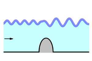
  $U$ in the opposite direction. A definition sketch of the coordinate system is shown in figure 1(a). The liquid is inviscid and incompressible, and the flow is assumed to be irrotational, thus allowing us to use a potential flow model.

Figure 1. ( $a$) Physical plane and ( $b$) parameter, or $\zeta$, plane.
The obstruction and the bottom downstream are assumed to have an arbitrary shape, which is defined by the function  $Y_b(S)$, where $S$ is the arc length coordinate, or by the slope of the bottom, $\delta _b = {\rm d}Y/{\rm d}S$,
 \begin{equation} \delta_b(X)=\arctan\frac{{\rm d} Y_b}{{\rm d} X}. \end{equation}
We introduce the complex velocity potential,  $W(Z) = \varPhi (X,Y) + {\rm i}\varPsi (X,Y)$, which consists of the velocity potential $\varPhi (X,Y)$ and the streamfunction $\varPsi (X,Y)$. Here, $Z = X + {\rm i}Y$. The boundary-value problem for the velocity potential can be written as follows:
 \begin{equation} \nabla^2 \varPhi = 0, \quad \nabla^2 \varPsi = 0, \end{equation}
in the liquid domain
 \begin{equation} \frac{\partial \varPhi}{\partial Y}=\frac{\partial \varPhi}{\partial X}\frac{{\rm d} Y_b}{{\rm d} X}, \quad \varPsi = 0, \end{equation}
on the bottom of the channel  $Y_b=Y_b(X)$
 \begin{equation} \rho\frac{V^2}{2}+\rho g Y + p_{ice}(X) + p_{ext}(X) = \rho\frac{U^2}{2}+\rho g H + p_\infty, \end{equation}
which is the dynamic boundary condition at the ice/liquid interface,  $Y=Y(X)$. Here, $V=|\boldsymbol {\nabla } \varPhi |$ is the velocity magnitude, $p_{ice} (X)$ is the hydrodynamic pressure at the ice/liquid interface and $P_\infty = P_a + \rho _i gh$ is its value at infinity; $p_a$ is the atmospheric pressure, $\rho _i$ is the density of ice, $h$ is the thickness of the ice sheet and $g$ is the gravitational acceleration, $p_{ext}(X)$ is the external pressure applied to the elastic sheet on the intervals $X_{P2}< X < X_{P1}$ and $X_{T1} < X < X_{T2}$ to provide a waveless interface far upstream and downstream; this will be discussed in the following.
The sought-for solution has the limit  $Y(X)_{X \rightarrow -\infty } = H$, where $H$ is the depth of the channel. The flow is steady; therefore, the value of the streamfunction at the interface is constant and equal to the flow rate across the channel
 \begin{equation} \varPsi=UH, \end{equation}
and the far-field condition
 \begin{equation} \boldsymbol{\nabla} \varPhi \rightarrow U, \quad X \rightarrow -\infty, \quad 0 \le Y \le H. \end{equation}
To complete the formulation of the boundary-value problem (2.2)–(2.4), an equation in the hydrodynamic pressure at the ice/liquid interface is needed. The elastic sheet is modelled using the Cosserat theory of hyperelastic shells (Plotnikov & Toland Reference Plotnikov and Toland2011)
 \begin{equation} p_{ice}=D^\prime \left(\frac{{\rm d}^2\kappa}{{\rm d}S^2}+\frac{1}{2}\kappa^3\right)+p_a , \end{equation}
where  $D^\prime ={Eh^3}/{12(1-\nu ^2)}$ is the flexural rigidity of the elastic sheet, $\kappa$ is the curvature of the interface, $E=5.0$ GPa is Young's modulus and $\nu =0.3$ is Poisson's ratio. Equation (2.7) corresponds to the assumption that the elastic sheet is inextensible and is not prestressed. It should be noted that the difference between the Cosserat theory and the Kirchhoff–Love plate model, in which the cube of the curvature term in (2.7) is omitted, is quite small due to the small curvature of the ice sheet before it starts breaking.
The interactions between the obstruction, the flow and the elastic sheet may generate waves that extend to both upstream and downstream infinity. However, the solutions with waves extending to upstream infinity are physically meaningless because they do not satisfy the radiation condition, which requires that there be no energy coming from infinity (Binder, Vanden-Broeck & Dias Reference Binder, Vanden-Broeck and Dias2009). To satisfy the radiation condition, or make the interface waveless far upstream, we apply an external pressure on the interval  $P_1 P_2$ (see figure 1a), which can be located as far as necessary to avoid its effect on the flow near the obstruction
 \begin{equation} p_{ext}= C_d V\frac{{\rm d}V}{{\rm d}X}, \end{equation}
where the coefficient  $C_d$ characterizes the wave attenuation on the interval $P_1 P_2$; it linearly increases from zero at point $P_1$ to some value $C_{up} > 0$ at point $P_2$ and then remains constant.
Now we recall that potential flows of an ideal fluid are reversible, i.e. changing the direction of the inflow velocity has no effect on the results. Alternatively, the flow region can be mirrored about the  $y$-axis without reversing the velocity direction. Therefore, to make our solution reversible, it is also necessary to provide a waveless interface far downstream. Similarly, the external pressure (2.8) is applied on the interval $T_1 T_2$ downstream. The coefficient $C_d$ changes from zero at point $T_1$ to some value $C_d=C_{dw}$ at point $T_2$ and then remains constant. The same wave attenuation technique was used by Semenov (Reference Semenov2021) for a similar problem, but with an infinite water depth.
To solve the problem, it is convenient to non-dimensionalize the variables. The velocity  $U$ and the depth of the channel $H$ are used as the reference quantities. Specifically, $x = X/H$ and $y = Y/H$, $s = S/H$, the thickness of the ice sheet $h$ is replaced with $h^* = h/H$, the bottom profile $y_b(x) = Y_b(X)/H$ and the interface profile $y(x) = Y(x)/H$. The velocity potential $\varPhi$ and the streamfunction $\varPsi$ are also normalized to the product $UH$. The normalized variables are denoted as $\phi = \varPhi /UH$ and $\psi = \varPsi /UH$. With these normalizations, the value of the streamfunction on the bottom of the channel is $\psi = 0$, and the value of the streamfunction at the interface is $\psi = 1$.
The non-dimensionalized dynamic boundary condition (2.4) takes the form
 \begin{equation} v^2=1 - \frac{2(y-1)}{F^2}- 2D\left(\frac{{\rm d}^2\kappa}{{\rm d}S^2}+\frac{1}{2}\kappa^3\right)- \frac{2C_d}{H}v\frac{{\rm d}v}{{\rm d}s}, \end{equation}
where
 \begin{equation} v=|\boldsymbol{\nabla} \phi|=V/U, \quad E_b=\frac{D^\prime}{\rho gH^4 }, \quad D=\frac{E_b}{ F^2}, \quad \kappa=\frac{{\rm d}\delta}{{\rm d}s}, \end{equation}
and
 \begin{equation} F=\frac{U}{\sqrt{gH}}, \end{equation}
is the Froude number based on the depth of the channel,  $\delta =\arcsin ({{\rm d}\kern 0.05em y}/{\rm d}s)=\beta +{\rm \pi}$ is the angle between the $X$-axis and the unit tangential vector $\boldsymbol {\tau }$ oppositely directed to the velocity direction $\beta$. Equation (2.9) contains the velocity magnitude along the interface $v$ and the wave elevation $y$ with its derivatives, which will be related in the following through the derived expression for the complex potential.
2.1. Dispersion relation
We examine a steady sine-like wavy interface of small steepness  $\delta _0$, or the slope of the interface can be represented as
 \begin{equation} \delta(s)={\rm Re}[ \delta_0\,{\rm e}^{{\rm i}kHs}], \end{equation}
where  $kH$ is the non-dimensional wavenumber. Upon differentiating equation (2.9) in the arc length coordinate $s$, we obtain
 \begin{equation} v^2\frac{{\rm d} \ln v}{{\rm d}s}={-}\left(\frac{1}{F^2} + D(kH)^4 \right)\delta. \end{equation}
For the case without an ice sheet ( $D = 0$), (2.13) becomes
 \begin{equation} v^2\frac{{\rm d} \ln v}{{\rm d}s}={-}\frac{\delta}{F^2}={-}\frac{kH}{\tanh kH}\delta, \end{equation}
where we used the relation between the Froude number and wavenumber for free-surface gravity waves in a channel of depth  $H$ (Kochin, Kibel & Roze Reference Kochin, Kibel and Roze1964). We assume that the velocity along the interface behaves in the same as for the free-surface case. From (2.13) and (2.14), we obtain the dispersion equation, which coincides, in particular, with that in the papers of Greenhill (Reference Greenhill1886) and Page & Părău (Reference Page and Părău2014)
 \begin{equation} \frac{kH}{\tanh kH} = \frac{1}{F^2} + D(kH)^4. \end{equation}
 The number of real roots of (2.15) depends on the value of the constant  $D$ and the Froude number $F$. It can have no roots, two roots or one root. These cases correspond to a subcritical flow (no roots), $F< F_{cr}$, a channel subcritical and ice supercritical flow (two roots), $F_{cr}< F<1$, and a channel supercritical flow, $F>1$.
The wavenumber vs the Froude number obtained from the solution of (2.15) is shown in figure 2 for various thicknesses of the ice sheet. It can be seen that, without an ice sheet ( $h=0$), each Froude number $F<1$ corresponds to one wavenumber. It tends to zero as the Froude number $F\rightarrow 1$. In the presence of an ice sheet, there is a minimal, or critical, Froude number $F_{cr}$, for which the solution of the dispersion equation exists. In the range $F_{cr}< F<1$, there are two wavenumbers, $k_{gr}$ and $k_{ice}$ corresponding to the gravity and elastic waves; the wavenumber $k_{ice} > k_{gr}$, or the elastic wave is shorter than the gravity wave. This range of the Froude number corresponds to the ice supercritical and channel subcritical flows. The larger the ice thickness, the smaller the wavenumber $k_{ice}$, and the critical Froude number $F_{cr} \rightarrow 1$. Thus, the interval $F_{cr} < F < 1$, in which both the gravity and the elastic waves may appear, reduces. For $F>1$, or for the channel supercritical flows, there is one root due to the elastic sheet. Since for $F>1$ the perturbations in the channel cannot extend upstream, we may expect the elastic wave to extend downstream. Usually, the dispersion equation (2.15) relates a wave frequency (or phase speed of a monochromatic wave moving in still water) to the wavenumber: $\omega ^2=k^2U^2$. In the present case, $U^2=F^2gH$; therefore, the frequency $\omega$ and the Froude number are related as $\omega ^2=k^2F^2gH$.

Figure 2. Wavenumber vs Froude number for different thicknesses of the ice sheet,  $h/H$.
2.2. Integral hodograph method
Finding the complex potential of the flow,  $w=w(z)$, directly is a complicated problem since the boundary of the flow region is unknown in advance. Instead, Joukowskii (Reference Joukowskii1890) and Michell (Reference Michell1890) proposed to introduce an auxiliary parameter plane, or $\zeta$-plane, which was typically chosen as the upper half-plane. Then, they considered two functions, which were the complex potential $w$ and the function
 \begin{equation} \omega ={-}\ln \left( \frac{1}{v_0} \frac{{\rm d}w}{{\rm d}z}\right)=\ln\frac{v}{v_0} - {\rm i}\beta, \end{equation}
both functions of the parameter variable  $\zeta$. Here, $v$ and $\beta$ are the velocity magnitude and direction, respectively; $v_0$ is the magnitude of the velocity on the free surface, which is assumed to be constant. When $w=w(\zeta )$ and $\omega (\zeta )$ are derived, the velocity and the flow region can be obtained in parametric form as follows:
 \begin{equation} \frac{{\rm d}w}{{\rm d}z}=\exp[-\omega(\zeta)], \quad z(\zeta)=z_0+\int_0^\zeta\left.\frac{{\rm d}w}{{\rm d}\zeta^\prime}\,\right/\frac{{\rm d}w}{{\rm d}z}\,{\rm d}\zeta^\prime, \end{equation}
where the function  $z(\zeta )$ is called the mapping function.
The Joukowskii–Michell method is capable of solving free-surface problems for flows over polygon-shaped bodies with a constant velocity on the free surface/interface (without gravity, surface tension, etc.). In this case the functions  $\omega (\zeta )$ and $w(\zeta )$ form polygon-shaped domains and can be found applying the Schwarz–Christoffel integral to find their conformal mapping into the upper half-plane.
An additional complexity arises when the slope of the body varies along the body contour or the velocity magnitude on the free surface/interface varies due to gravity, surface tension, etc. On these parts of the flow boundary, the boundary conditions are of different types: on the solid part of the boundary, the velocity direction is determined by the slope of the body; on the free surface/interface, the velocity magnitude can be obtained from the Bernoulli equation. This is a so-called mixed boundary-value problem for a complex function.
If the upper half-plane is chosen as the region of the parameter variable and the whole real axis corresponds to the free surface or the body surface, then Schwarz's integral formula or Cauchy's integral formula can be applied to determine the desired complex function. This approach was applied by Forbes & Schwartz (Reference Forbes and Schwartz1982) for solving free-surface flow over a semicircular obstruction. In order to use Cauchy's integral formula, they introduced an image flow symmetric about the  $x$-axis and were able to formulate a uniform boundary-value problem for the complex function ${\rm d}\zeta /{\rm d}w$. By using Cauchy's integral formula and the dynamic boundary condition, they obtained an integro-differential equation in the complex function ${\rm d}\zeta /{\rm d}w$.
In this paper, we use a different integral formula (Semenov & Iafrati Reference Semenov and Iafrati2006; Semenov & Cummings Reference Semenov and Cummings2007) that allows us to determine a complex function based on the values of its argument and magnitude given on the real and imaginary axes of the first quadrant, respectively. Therefore, we chose the first quadrant as the region of the parameter variable  $\zeta = \xi + {\rm i}\eta$ (instead of a half-plane) shown in figure 1( $b$). The parameter region corresponds to the liquid domain in the physical plane $z = x+{\rm i}y$ shown in figure 1( $a$): the real axis corresponds to the bottom of the channel, and the imaginary axis corresponds to the interface. The conformal mapping theorem allows us to arbitrarily choose the location of three points $O(O')$ ( $\zeta = 0$) $B$ (
$B$ ( $\zeta = 1$) and $D(D')$ ( $\zeta = \infty$), as shown in 1( $b$). Then, the locations of points $A$ (
$A$ ( $\zeta = a$) and $C$ (
$C$ ( $\zeta = c$) are unknown and have to be determined using additional physical considerations.
The complex velocity function on the bottom of the channel and that at the interface are unknown a priori. At this stage, we assume that these functions are known as functions of the parameter variables:  $v(\eta ) = |{\rm d}w/{\rm d}z|$ is known as a function of the coordinate $\eta$ along the imaginary axis in the $\zeta$-plane; $\chi (\xi ) = \arg ({\rm d}w/{\rm d}z)$ is a known function of the coordinate $\xi$ along the real axis of the first quadrant in the $\zeta$-plane. These functions will be determined later using the dynamic and kinematic boundary conditions at the interface and on the bottom, respectively. Using the above definitions, we can write the following boundary-value problem for the complex velocity function:
 \begin{gather} \left| \frac{{\rm d}w}{{\rm d}z} \right|_{\zeta={\rm i}\eta} =v (\eta), \quad 0\le\eta<\infty, \end{gather}
 \begin{gather}\arg \left(\left. \frac{{\rm d}w} {{\rm d}z}\right|_{\zeta=\xi} \right) = \chi(\xi), \quad 0\le\xi<\infty. \end{gather}
By using Chaplygin's singular point method (Gurevich Reference Gurevich1965, §5 Chapter 1), the following integral formula can be obtained for solving the mixed boundary-value problem (2.18) and (2.19) (Semenov & Iafrati Reference Semenov and Iafrati2006):
 \begin{align} \frac{{\rm d}w}{{\rm d}z} = v_\infty \exp \left[\frac{1}{{\rm \pi} }\int_\infty^0 \frac{{\rm d}\chi}{{\rm d}{\xi }}\ln \left( {\frac{\zeta + \xi}{\zeta - \xi}} \right){\rm d}{\xi } - \frac{{\rm i}}{{\rm \pi} }\int_0^\infty \frac{{\rm d}\ln v}{{\rm d}{\eta }}\ln \left( {\frac{\zeta - {\rm i}{\eta }}{\zeta + {\rm i}{\eta }}} \right){\rm d}{\eta } + {\rm i}\chi_\infty \right], \end{align}
where  $v_\infty =\lim _{\eta \to \infty } v(\eta )$ and $\gamma _\infty =\lim _{\xi \to \infty } \chi (\xi )$. An alternative way of derivation of the above integral formula is presented by Semenov & Cummings (Reference Semenov and Cummings2007). It can easily be verified that, for $\zeta = \xi$, the argument of the function ${\rm d}w/{\rm d}z$ is the function $\chi (\xi )$, while for $\zeta ={\rm i}\eta$ the magnitude of ${\rm d}w/{\rm d}z$ is the function $v(\eta )$, i.e. the boundary conditions (2.18) and (2.19) are satisfied.
The argument of the complex velocity is determined by the slope of the bottom,  $\delta _b$, or $\chi (\xi )=-\delta _b(\xi )$, which at points $A$ and $C$ undergoes a step change due to the corners at points $A$ and $C$, as can be seen in figure 1( $a$). We introduce a continuous function $\gamma (\xi )$ that changes from the value $\gamma (a)=0$ at point $A$, ( $\xi =a$), to the value $\gamma (c)=-{\rm \pi}$ at point $C$, ( $\xi =c$), and further may vary continuously along the bottom
 \begin{equation} \chi(\xi) = \left\{ \begin{array}{ll} 0, & 0 < \xi < a, \\ -{\rm \pi}/2 -\gamma(\xi) , & a \leq \xi \leq c, \\ -{\rm \pi} - \gamma(\xi) , & c < \xi < \infty. \end{array} \right. \end{equation}
The function  $\chi (\xi )$ has two jumps: at point $A$,
$A$,  $\varDelta _A = -{\rm \pi} /2$ and at point $C$,
$C$,  $\varDelta _C = -{\rm \pi} /2$. The function $\gamma (\xi )$ differs from the function $\delta _b(\xi )$ only by a constant; therefore, ${\rm d}\gamma /{\rm d}\xi ={\rm d}\delta _b/{\rm d}\xi$. Substituting (2.21) into (2.19), evaluating the integrals over the step changes of the function $\chi (\xi )$ and using ${\rm d}\gamma /{\rm d}\xi ={\rm d}\delta _b/{\rm d}\xi$, we obtain the expression for the complex velocity as
 \begin{align} \frac{{\rm d}w}{{\rm d}z} & = v_0\sqrt{\frac{a - \zeta}{a + \zeta}\frac{c - \zeta}{c + \zeta}}\exp \left[- \frac{1}{{\rm \pi} }\int_a^\infty \frac{{\rm d}\delta_b}{{\rm d}{\xi}}\ln \left( {\frac{{\xi } - \zeta }{{\xi} + \zeta }} \right){\rm d}{\xi } \right.\nonumber\\ &\quad - \left. \frac{{\rm i}}{{\rm \pi} }\int_0^\infty \frac{{\rm d}\ln v}{{\rm d}{\eta }}\ln \left( {\frac{{\rm i}{\eta } - \zeta }{{\rm i}{\eta } + \zeta }} \right){\rm d}{\eta } \right], \end{align}
where  $v_0=1$ is the velocity magnitude at point $O$. Here, we used $\arg (\zeta -{\rm i}\eta )=\arg ({\rm i}\eta -\zeta )-{\rm \pi}$ for the second integral.
2.3. Derivative of the mapping function,  ${\rm d}z/{\rm d}w$

On the bottom of the channel the streamfunction  $\psi \equiv 0$, and at the interface $\psi \equiv 1$ as follows from the boundary conditions (2.3) and (2.5), while the potential varies from $-\infty$ to $+\infty$. Thus, the domain of the complex potential $w = \phi +{\rm i}\psi$ is the infinite strip $-\infty < \phi <\infty$ of unit width, $0 \leq \psi \leq 1$. Due to the simplicity of the domain of $w$, we can use conformal mapping to immediately write the complex potential $w$ as a function of the parameter variable $\zeta$
 \begin{equation} w(\zeta) = \frac{2}{\rm \pi}\ln \zeta. \end{equation}
 The complex potential (2.23) is a logarithmic function of  $\zeta$, or $\zeta$ exponentially depends on the complex potential $w = \phi +{\rm i}\psi$. The arc length coordinates $s_b \sim \phi$ and $s \sim \phi$ along the bottom and the interface, respectively. This causes difficulties in computations for a length of the computational region larger than $5H$. We can resolve the logarithmic singularity if we eliminate the parameter variables $\zeta$, $\xi$ and $\eta$ from (2.22) using the expressions
 \begin{equation} \left.\begin{array}{c} \zeta=\exp({\rm \pi} w/2), \quad -\infty \leq \phi \le \infty, \quad 0\leq \psi \leq 1, \\ \eta=\exp({\rm \pi}\phi/2 ), \quad -\infty \leq \phi \le \infty, \quad \psi =1, \\ \xi=\exp({\rm \pi}\phi/2), \quad -\infty \leq \phi \le \infty, \quad \psi =0. \end{array} \right\} \end{equation}
 By substituting (2.24) into (2.22), we obtain the complex velocity as a function of the complex potential  $w$, the inverse function of which is the derivative of the mapping function, $z=z(w)$
 \begin{align} \frac{{\rm d}z}{{\rm d}w} & = \frac{1}{v_0}\sqrt{\frac{a + {\rm e}^{w^\prime}}{a - {\rm e}^{w^\prime}}\frac{c + {\rm e}^{w^\prime}}{c - {\rm e}^{w^\prime}}}\exp \left[\frac{1}{{\rm \pi} }\int_{\phi^\prime_A}^\infty \frac{{\rm d}\delta_b}{{\rm d}{\phi^\prime}} \ln \left(\frac{{\rm e}^{\phi^\prime} - {\rm e}^{w^\prime}}{{\rm e}^{\phi^\prime} + {\rm e}^{w^\prime}}\right){\rm d}{\phi^\prime} \right. \nonumber\\ &\quad +\left. \frac{{\rm i}}{{\rm \pi} }\int_{-\infty}^\infty \frac{{\rm d}\ln v}{{\rm d}{\phi^\prime }}\ln \left(\frac{{\rm i}{\rm e}^{\phi^\prime} - {\rm e}^{w^\prime}}{{\rm i}{\rm e}^{\phi^\prime} + {\rm e}^{w^\prime}}\right){\rm d}{\phi^\prime} \right], \end{align}
where  $w^\prime ={\rm \pi} w/2$ and $\phi ^\prime ={\rm \pi} \phi /2$. The integrals containing functions
 \begin{equation} \ln \left(\frac{{\rm e}^{\phi^\prime} - {\rm e}^{w^\prime}}{{\rm e}^{\phi^\prime} + {\rm e}^{w^\prime}}\right), \quad \ln \left(\frac{{\rm i}{\rm e}^{\phi^\prime} - {\rm e}^{w^\prime}}{{\rm i}{\rm e}^{\phi^\prime} + {\rm e}^{w^\prime}}\right), \end{equation}
exponentially decay as the difference  $|\phi ^\prime - w^\prime |$ increases. The integration of (2.25) along $-\infty < \phi < \infty$, $\psi = 1$, in the $w$-plane gives the interface $OD$; its integration along $-\infty < \phi < \infty$, $\psi = 0$ gives the bottom surface. The parameters $a=\exp ({\rm \pi} \phi _A/2)$ and $c=\exp ({\rm \pi} \phi _C/2)$. The potentials $\phi _A$ and $\phi _C$, and the functions $\delta _b (\phi )$ and $v(\phi )$ are unknown and have to be determined from physical considerations and the boundary conditions.
2.4. Integro-differential equations in the functions $\delta _b(\phi )$

By using the derivative of the mapping function (2.25) we can obtain the arc length coordinate  $s_b$ as a function of the potential $\phi$
 \begin{equation} s_b(\phi) =\int_0^{\phi}\frac{{\rm d}s_b}{{\rm d}\xi} \,{\rm d}\phi^{\prime}, \end{equation}
where
 \begin{align} \frac{{\rm d}s_b}{{\rm d}\phi} &= \left|\frac{{\rm d}z}{{\rm d}w}\right|_{w=\phi} = \frac{1}{v_0}\sqrt{\left|\frac{a + {\rm e}^{\phi^\prime}}{a - {\rm e}^{\phi^\prime}}\frac{c + {\rm e}^{\phi^\prime}}{c - {\rm e}^{\phi^\prime}}\right|} \exp \left\{\frac{1}{{\rm \pi} }\int_{\phi_A}^\infty \frac{{\rm d}\delta_b}{{\rm d}\phi^{\prime\prime}} \ln \left|\frac{{\rm e}^{\phi^{\prime\prime}} - {\rm e}^{\phi^\prime}}{{\rm e}^{\phi^{\prime\prime}} + {\rm e}^{\prime\prime}}\right|{\rm d}\phi^{\prime\prime} \right. \nonumber\\ &\quad +\left. \frac{1}{{\rm \pi} }\int_{-\infty}^\infty \frac{{\rm d}\ln v}{{\rm d}\phi^{\prime\prime}} [{\rm \pi}-2\tan^{{-}1} ( {\rm e}^{\phi^{\prime\prime} - \phi^\prime})]\,{\rm d}\phi^{\prime\prime} \vphantom{\left|\frac{{\rm e}^{\phi^{\prime\prime}} - {\rm e}^{\phi^\prime}}{{\rm e}^{\phi^{\prime\prime}} + {\rm e}^{\prime\prime}}\right|}\right\}, \end{align}
and  $\phi ^\prime ={\rm \pi} \phi /2$.
The bottom shape is given by the slope of the bottom,  $\delta _b=\delta _b(s_b)$. By making the change of variables $s_b=s_b(\phi )$, we obtain the following integro-differential equation in the function $\delta _b(\phi )$:
 \begin{equation} \frac{{\rm d}\delta_b}{{\rm d}\phi} = \frac{{\rm d}\delta_b}{{\rm d}s}\frac{{\rm d}s_b}{{\rm d}\phi}, \end{equation}
where  ${\rm d}s_b/{\rm d}\phi$ is determined from the above equation, which also contains the function ${\rm d}\delta _b/{\rm d}\phi$. The parameters $\phi _A$ and $\phi _C$ are determined from the given arc length of the obstruction $ABC$. In view of (2.27)
 \begin{equation} s_{AB} = s_b(\phi_A), \quad s_{BC} = s_b(\phi_C), \end{equation}
where  $s_{AB}$ and $s_{BC}$ are the arc lengths of the parts $AB$ and $BC$ of the obstruction.
2.5. Determination of the function $v(\phi )$

The velocity magnitude at the interface is determined using the dynamic boundary condition (2.9), which contains the interface shape  $y(s)$ and curvature with its higher derivatives. The ice/liquid interface is obtained by integrating the derivative of the mapping function (2.25) along the upper side of the strip in the $w$-plane, or $w=\phi +{\rm i}$, it takes the form
 \begin{equation} x(\phi) + {\rm i}y(\phi) = x_O + {\rm i}H + \int_{-\phi^\ast}^{\phi} \left(\frac{{\rm d}z}{{\rm d}w}\right)_{w=\phi+{\rm i}}\,{\rm d}\phi, \end{equation}
where the coordinate of point  $x_O$ is obtained by integrating the derivative of the mapping function (2.25) along the lower side of the strip in the $w$-plane, which corresponds to the bottom of the channel
 \begin{equation} x_O= \int_0^{-\phi^\ast}\left(\frac{{\rm d}z}{{\rm d}w}\right)_{w=\phi}\,{\rm d}\phi. \end{equation}
Here,  $-\phi ^{\ast }$ and $\phi ^{\ast }$ are the lower and the upper boundary of the computational region; the channel in the physical plane is truncated, and the flow outside the computational region, $|\phi |>\phi ^{\ast }$, is assumed to be uniform. The arc length coordinate along the interface is
 \begin{equation} s(\phi) = \int_0^{\phi} \frac{{\rm d}\phi}{v(\phi)}. \end{equation}
It would be possible to determine the slope of the interface using the derivative of the mapping function (2.25)
 \begin{equation} \delta(\phi) = {\rm Im} \left[ \ln\left( \frac{{\rm d}z}{{\rm d}w}\right)_{w=\phi+{\rm i}} \right], \end{equation}
and then evaluate the curvature of the interface and its first and second derivatives by differentiating the equation
 \begin{equation} \kappa= \frac{{\rm d}\delta}{{\rm d}s}=\frac{{\rm d}\delta}{{\rm d}\phi}\frac{{\rm d}\phi}{{\rm d}s}. \end{equation}
However, when differentiating the function  $\delta (\phi )$ with respect to $\phi$, the order of singularity in the integrand of the second integral in (2.25) increases. By substituting the $y$-coordinate of the interface and the second derivative of the curvature into the dynamic boundary condition (2.9), we obtain a very complicated hypersingular integral equation in the function $v(\phi )$, whose numerical solution requires special treatments.
Instead of solving the hypersingular integral equation, we use another numerical method based on the spline approximation of the interface to evaluate its curvature and higher derivatives. In discrete form, the solution is sought on two fixed sets of points: a set  $-\phi ^\ast < \phi _j < \phi ^\ast$, $j=1,\ldots, N$ corresponding to the bottom of the channel and a set $-\phi ^\ast < \phi _i < \phi ^\ast$, $i = 1,\ldots, M$ corresponding to the interface; both sets of points $\phi _j$ and $\phi _i$ monotonically increase.
We chose a fifth-order spline, which provides continuous derivatives along the interface up to the fourth derivative appearing in the pressure coefficient due to the ice sheet,
 \begin{align} y(s) = y_k + a_{1,k}(s - s_{k-1}) + \cdots + a_{n,k}(s - s_{k-1})^n, \quad s_{k-1} < s < s_k, \ k=1,\ldots,\bar{K}, \end{align}
where nodes  $s_k=s_{{\rm i}(k)}$ and $y_k = y_{{\rm i}(k)}$, ${\rm i}(k)=4k-3$, $k=1,\ldots,\bar {K}$, $\bar {K}=M/4$ are chosen as every fourth point on the set of the discrete points $s_i = s(\phi _i)$ and $y_i=y(\phi _i)$ determined from (2.31) and (2.33). The curvature and its derivatives are obtained by differentiating (2.34)
 \begin{equation} \delta=\arcsin y^\prime, \quad \kappa=\frac{y^{\prime\prime}}{\sqrt{1-y^{\prime 2}}}, \quad \frac{{\rm d}\kappa}{{\rm d}s}=\frac{y^\prime y^{\prime\prime 2}-y^{\prime\prime\prime}(y^{\prime 2}-1)}{(1-y^{\prime 2})^{3/2}}, \ldots. \end{equation}
By applying the dynamic boundary condition (2.9) at the points  $\phi _k$, $k=1,\ldots,\bar {K}$, we can obtain the following system of nonlinear equations:
 \begin{equation} G_k(\bar{V})=c_{pk}(\bar{V})-c_{pk}^{ice}(\bar{V})=0, \quad k=1,\ldots, \bar{K}, \end{equation}
where  $\bar {V}=(v_1,\ldots,v_{\bar {K}})^{T}$ is the vector of the unknown velocities $v_k$ at the nodes $s_k$
$s_k$
 \begin{gather} c_{pk}(\bar{V})=1-v_k^2-\frac{2[y_k(\bar{V})-1]}{F^2} - C_dv_k\left(\frac{{\rm d}v}{{\rm d}\kern 0.06em x}\right)_k, \end{gather}
 \begin{gather}c_{pk}^{ice}(\bar{V})=2D\left[ \left( \frac{{\rm d}^2\kappa}{{\rm d}s^2} \right)_k +\frac{1}{2}\kappa_k^3\right], \end{gather}
are the hydrodynamic pressure coefficient and the pressure coefficient due to the elastic sheet, respectively. The wave attenuation intervals are chosen to be  $x_{P1}-x_{P2}=2\lambda _{gr}$ and $x_{T2}-x_{T1}=3\lambda _{gr}$, where $\lambda _{gr}$ is the wavelength determined from the dispersion relation. The coefficients $C_{up}$ and $C_{dw}$ are chosen in the interval from $0.2\lambda _{gr}$ to $0.4\lambda _{gr}$ to effectively damp both the elastic and the gravity wave upstream and downstream, respectively.
The system of (2.38) is solved using Newton's method. The Jacobian of the system is evaluated numerically using the central difference with  $\Delta v_k=10^{-8}$. At each evaluation of the function $G_k(\bar {V})$, the integro-differential equation (2.29) together with (2.28) and (2.30) is solved using the method of successive approximations, which in the discrete form becomes
 \begin{equation} \frac{(\Delta \delta_b )_j^{(m+1)}}{\Delta\phi_j}=\frac{\delta_b(s_{bj}^{(m)}) - \delta_b(s_{b(j-1)}^{(m)})}{\Delta \phi_j}, \end{equation}
where the arc length along the body,  $s^{(m)}_{bj}=s_b^{(m)}(\phi _j)$ is evaluated using (2.27) with $(\Delta \delta _b )_j^{(m)}/{\Delta \xi _j}$ known at the $m$ iteration. The iteration process converges very fast. After $5$ to $10$ iterations, the error is below a prescribed tolerance of $10^{-6}$. The parameters $a$ and $c$ are obtained as
 \begin{equation} a = \exp({\rm \pi}/2\phi_A), \quad c=\exp({\rm \pi}/2\phi_C), \end{equation}
where  $\phi _A$, and $\phi _C$ are determined from (2.30). From $5$ to $20$ iterations are necessary to get a converged solution. All solutions, say $\overline {V^\ast }$, reported here satisfied the condition
 \begin{equation} \frac{1}{\bar{K}}\sum_1^{\bar{K}}|G_k(\overline{V^\ast})|<10^{{-}6}, \end{equation}
which is regarded as giving a sufficiently accurate solution of the nonlinear equations.
In the first iteration, the functions  $v(\phi )$, $s_b(\phi )$, $\delta _b(\phi )$, and the parameters $\phi _A$ and $\phi _C$ are given as follows: $v^{(1)}(\phi ) \equiv 1$, $s^{(1)}_b(\phi )=\phi$, $\phi ^{(1)}_A=s_{AB}$, $\phi ^{(1)}_C=s_{BC}$ and
 \begin{equation} \delta^{(1)}_b(\phi) = \left\{\begin{array}{ll} {\rm \pi}/2, & -\infty < \phi \leq \phi_A, \\ {\rm \pi}/2 -{\rm \pi} (\phi - \phi_A)/(\phi_C - \phi_A), & \phi_A \leq \phi \leq \phi_C, \\ -{\rm \pi}/2 , & \phi_C \leq \phi < \infty. \end{array} \right. \end{equation}
Then, the next iteration starts from solving integro-differential equation (2.29).
3. Results and discussion
3.1. Numerical approach
The number of nodes on the bottom and at the interface is chosen in the ranges  $200 < N < 400$ and $400 < M < 4000$, respectively, based on the requirement to provide at least $12$ nodes $s_k$ within the shorter wavelength and to get a reasonably accurate converged solution. The computational time varies form few minutes for $M=400$ to approximately $30$ min for $M=4000$ using a desktop Precision Tower T7920.
The integrals appearing in (2.25) are evaluated analytically using points of discretization of the real and imaginary axes of the first quadrant in the  $\zeta$-plane, $\xi _j=\exp ({\rm \pi} \phi _j/2)$ and $\eta _i=\exp ({\rm \pi} \phi _i/2)$, a linear interpolation of the functions $\delta _b(\xi )$ on the intervals $(\xi _{j-1}, \xi _j)$ and the function $\ln v(\eta )$ on the intervals $(\eta _{i-1}, \eta _i)$
 \begin{gather} \frac{1}{{\rm \pi} }\int_{\xi_{j-1}}^{\xi_j}\frac{{\rm d}\delta_b}{{\rm d}{\xi}}\ln \left( {\frac{{\xi } - \zeta}{{\xi} + \zeta}} \right){\rm d}{\xi } = \Delta\delta_{bj} a_j(\zeta), \end{gather}
 \begin{gather}\frac{1}{{\rm \pi} }\int_{-{\eta_{i-1}}}^{\eta_i} \frac{{\rm d}\ln v}{{\rm d}\eta}\ln \left(\frac{{\rm i}\eta - \zeta}{{\rm i}\eta + \zeta } \right){\rm d}{\xi } = \Delta (\ln v)_i b_i(\zeta), \end{gather}
where
 \begin{gather} \Delta\delta_{bj} = \delta_b(\xi_j) - \delta_b(\xi_{j-1}), \end{gather}
 \begin{gather}a_j(\zeta) = \frac{1}{{\rm \pi}\Delta\xi_j}\int_{\xi_{j-1}}^{\xi_{j}}\ln \left(\frac{\xi - \zeta}{\xi + \zeta } \right){\rm d}{\xi }, \end{gather}
 \begin{gather}\Delta (\ln v)_i=\ln v_i - \ln v_{i-1} =\ln \frac{v_i}{v_{i-1}}, \end{gather}
 \begin{gather}b_i(\zeta) =\frac{1}{{\rm \pi}\Delta\eta_i}\int_{\eta_{i-1}}^{\eta_{i}}\ln \left(\frac{{\rm i}\eta - \zeta}{{\rm i}\eta + \zeta } \right){\rm d}{\eta}. \end{gather}
The integral in the above equation can be easily evaluated, and the result is a non-singular expression for the functions  $a_j(\zeta )$ and $b_j(\zeta )$. By substituting (2.24) into (3.1) and (3.2) we can evaluate the integrals in (2.25).
3.2. Verification of the numerical approach
For verification purposes we compare the results predicted by the present nonlinear solution with the nonlinear theory (Page & Părău Reference Page and Părău2014) based on the boundary-integral method for the case of a hydraulic fall. Page & Părău (Reference Page and Părău2014) considered the hydraulic fall solution for which the depth of liquid upstream is greater than downstream. The flow is assumed to be uniform in the far field as  $|x| \rightarrow \infty$, with a constant depth $H$ and velocity $U$ downstream and a constant depth $H_{up} > H$ and velocity $U_{up}< U$ upstream of the obstruction on the bottom of the channel.
Applying Bernoulli's equation in the far fields  $|x|\rightarrow \pm \infty$ and using the conservation mass equation, the parameters upstream and downstream are related in non-dimensional form as follows (Dias & Vanden-Broeck Reference Dias and Vanden-Broeck2004):
 \begin{equation} \frac{1}{2} - \frac{1}{2} \gamma^{*2} + \frac{1}{F^2} - \frac{1}{F^2\gamma^{*2}} = 0, \end{equation}
where  $\gamma ^\ast =U_{up}/U$.
Page & Părău (Reference Page and Părău2014) considered a cosine-squared profile of the bottom of the channel including two obstructions as follows:
 \begin{equation} y_b(x) = \left\{\begin{array}{ll} 2A_1 \cos^2\left(\dfrac{{\rm \pi}(x+x_1)}{2L_1}\right), & -L_1< x< x+x_1< L_1, \\ 2A_2 \cos^2\left(\dfrac{{\rm \pi} x}{2L_2}\right), & -L_2< x< x< L_2, \\ 0, & \text{otherwise.} \end{array} \right. \end{equation}
The heights and half-lengths of the submerged obstructions are defined by  $2A_i$ and $L_i$ ( $i=1,2$), respectively. The separation constant $x_1$ describes the central position of the additional obstruction. In the case of just a single submerged obstruction, $A_1$ is taken to be zero.
The hydraulic fall profiles over an obstruction predicted by the present solution are compared with the results by Page & Părău (Reference Page and Părău2014) in figure 3 for two cases with Froude number  $F = 1.367$ and $F = 1.345$. It can be seen that the results predicted by the present method and those by Page & Părău (Reference Page and Părău2014) coincide.

Figure 3. Hydraulic fall profiles over a single submerged obstruction of height  $2A_2=0.1$ and length $L_2=6$; $E_b = 0.5$, $F = 1.367$, $\gamma ^\ast = 0.649$ (solid circles); $E_b = 0.1$, $F = 1.345$, $\gamma ^\ast = 0.664$ (solid squares); lines and symbols correspond to the present solution and Page & Părău (Reference Page and Părău2014), respectively.
An additional verification is performed for the case of two obstructions on the bottom. In the absence of a thin ice sheet, placing an additional obstruction downstream of the hydraulic fall in the pure gravity case can result in a train of trapped waves between the two obstructions (Dias & Vanden-Broeck Reference Dias and Vanden-Broeck2004). Page & Părău (Reference Page and Părău2014) predicted trapped waves in the presence of an ice sheet. The interface profile and the bottom shape for the case of an additional obstruction centred at  $x=20$ is shown in figure 4 for the present solution (solid line) and Page & Părău (Reference Page and Părău2014) (dashed line and solid symbols). The Froude number $F_{cr}$ is found as part of the solution using the additional condition of the absence of a wave downstream. If this condition is not applied and the Froude number $F>1$ is given, a wave downstream of the second obstruction can be observed. This will be discussed later in the following. An agreement between the present results and those by Page & Părău (Reference Page and Părău2014) verifies the calculation code.

Figure 4. Trapped wave at the ice/liquid interface (the solid line corresponds to the present calculations; the dashed line with symbols corresponds to Page & Părău (Reference Page and Părău2014)) for the bottom profile including two obstructions (blue line):  $2A_2=0.2$ and width $2L_2=6.4$ and an additional obstacle with $2A_1 =0.16$ and $2L_1=6.4$ placed at $x_1 = 20$; the Froude number $F =1.5373$ and $\gamma ^\ast = 0.545$ are found as part of the solution, and $E_b=0.5$.
3.3. Subcritical flows, $F< F_{cr}$

For Froude numbers  $F < F_{cr}$, (2.15) has only complex roots, which correspond to decaying perturbations of the interface caused by the obstruction on the bottom. In figure 5( $a$), the interface profiles for obstruction height $R/H =0.2$ and thickness of the ice elastic sheet $h/H=0.01$ are shown for different Froude numbers approaching the critical Froude $F_{cr}=0.864$. It can be seen that the interface shape is symmetric about the $y$-axis and the wave decays; the trough of the wave is located just above the obstruction, and it gets deeper as the Froude number approaches the critical value. This situation is different from that for the free-surface flows without an elastic sheet, for which the free surface is flat upstream and exhibits a wave downstream of the obstruction. Thus, for $F < F_{cr}$, the elastic sheet suppresses the waves downstream and perturbs the flow near the obstruction. It was found that for $R/H =0.2$ and Froude $0.65< F< F_{cr}$ the solution fails to converge, or $F=0.65$ is the maximal value.

Figure 5. ( $a$) The interface shape and ( $b$) the pressure coefficient along the interface for obstruction height $R/H = 0.2$, ice thickness $h/H=0.01$ and a subcritical flow: Froude number $F=0.65$ (solid line), $F=0.6$ (dashed line), $F=0.5$ (dotted line).
The interface profiles for different heights of the obstruction and the maximal value of the Froude number for each height are shown in figure 6: for height  $R/H = 0.32$, the maximal Froude number is $F=0.5$; for $R/H = 0.17$, $F=0.7$; and for $R/H = 0.06$, $F=0.83$. As the height of the obstruction further decreases, the maximum Froude number approaches the critical Froude number $F_{cr}=0.864$. It can be seen from figure 6( $a$) that the smaller the height of the obstruction, the smaller the deflection of the interface corresponding to the onset of convergence of the solution. Therefore, we can conclude that a large height of the obstruction or a large deflection of the ice/liquid interface itself does not prevent the convergence of the solution.

Figure 6. ( $a$) The interface shape and ( $b$) the pressure coefficient along the interface corresponding to the onset of convergence of the subcritical solution for ice thickness $h/H=0.01$: $F=0.5$, $R/H=0.32$ (solid line); $F=0.7$, $R/H=0.17$ (solid line); $F=0.83$, $R/H=0.06$ (solid line); the critical Froude number $F_{cr}=0.8636$.
The behaviour of the average error (2.43) and the velocity magnitude at the trough is shown in figure 7 (the left and right axes, respectively) for two slightly different heights of the obstructions. The initial velocity at the interface is set to  $v(\phi )\equiv 1$. At the beginning of the iterations, the velocity magnitude at the trough increases linearly for both cases due to the given restriction of the velocity increment. For $R/H=0.32$, the average error gradually decreases and the velocity at the trough tends to some value, while for $R/H=0.33$ both the error and velocity magnitude oscillate without any tendency to converge.

Figure 7. Convergence of the iterations for Froude number  $F=0.5$ and two heights of the obstruction, $R/H=0.32$ (red line) and $R/H=0.33$ (blue line); the left axis corresponds to the average error in the dynamic boundary condition (solid lines); the right axis corresponds to the velocity magnitude at the trough (dashed lines).
3.4. Ice supercritical – channel subcritical flows, $F_{cr}< F<1$

In this range of the Froude number, the dispersion relation (2.15) has two real roots: one root,  $k_{gw}$, is the wavenumber corresponding to the gravity wave (since its value is close to the wavenumber corresponding to the free-surface gravity waves), and the other root, $k_{ice}$, is caused by the elastic wave. Both waves may extend to infinity downstream and upstream. In order to examine how the introduced attenuation regions affect the solution, we compare in figure 8 the ice/liquid interfaces corresponding to two cases: for the first case, the computational region starts at $x_{P2}=-8\lambda _{gw}$ and ends at $x_{T2}=8\lambda _{gw}$ with attenuation zone length $L_{P1P2}=4\lambda _{gw}$ and $L_{T1T2}=3\lambda _{gw}$; for the second case, it starts at $x_{P2}=-10\lambda _{gw}$ and ends at $x_{T2}=9\lambda _{gw}$ with the same length of the attenuation zones. For both cases, the attenuation coefficients are $C_{up}=0.14\lambda _{gw}$ and $C_{dw}=0.4\lambda _{gw}$; for both cases, the Froude number $F=0.8$, $R/H=0.11$ and the ice thickness $h/H=0.005$, for which the critical Froude number $F_{cr}=0.6935$. From the dispersion relation (2.15), the wavenumbers are obtained: $k_{gw}=1.4252$ ( $\lambda _{gw}=4.409$) and $k_{ice}=4.0757$ ( $\lambda _{ice}=1.542$). The number of nodes of the spline $\bar {K}$ is chosen to provide at least 12 nodes within the shorter ice wave $\lambda _{ice}$. Then, the total number of nodes for the first case, $x_{T2} - x_{P2}=16\lambda _{gw}$, is obtained as $\bar {K}=12*16\lambda _{gw}/\lambda _{ice}\approx 550$, and the total number of discretization points at the interface is $M=4\bar {K}=2200$. For the second case, the length of the computational region $x_{T2} - x_{P2}=19\lambda _{gw}$, and $\bar {K}\approx 650$ and $M=2600$.

Figure 8. The ice/water interface for Froude number  $F=0.8$, obstruction height $R/H=0.11$ and different lengths of the computational region: $16\lambda _{gw}$ (red line); $19\lambda _{gw}$ (blue line). The dashed lines indicate the length and location of the attenuation zones.
The red and blue solid lines in figure 8 correspond to the first case and the second case, respectively. The dashed lines indicate the location and the length of the attenuation zones for each case. It can be seen that the red and blue lines coincide in the range of  $-4< x\lambda _{gw}< 5$ where the attenuation term in the dynamic boundary condition (2.9) is equal to zero ( $C_d=0$).
As the Froude number  $F\rightarrow 1$, the ratio $\lambda _{gw}/\lambda _{ice}=k_{ice}/k_{gw}\rightarrow \infty$ since the gravity wave number $k_{gw}\rightarrow 0$. In this case, the required number of discretization points also tends to infinity, thus causing computational difficulties. The computational analysis starts with $F=0.9$ and then gradually approaches the critical Froude number $F_{cr}=0.6935$; the ice thickness $h/H=0.005$. The wavelengths of the gravity and the elastic wave are $\lambda _{gw}=7.250$ and $\lambda _{ice}=1.344$, and their ratio $\lambda _{gw}/\lambda _{ice}=5.394$.
Figure 9 shows ( $a$) the interface profile, ( $b$) the bending moment and ( $c$) the pressure coefficient along the interface for two heights of the obstruction: $R/H=0.05$ (red line) and $0.07$ (blue line), Froude number $F=0.9$ or $F/F_{cr}=1.30$ and ice thickness $h/H=0.005$. This ratio is relatively large in terms of the interaction between the gravity and the elastic wave, which is quite weak. For $R/H=0.05$ the interface is almost flat upstream, or the oscillations of the elastic wave are invisible, although its contribution to the bending moment and the pressure coefficient is significant. For a larger height, $R/H=0.07$, the wave amplitude of the interface upstream becomes visible, but it is still much lower than the amplitude of the interface downstream corresponding to the gravity wave
 \begin{equation} F_{loc} = \frac{v(x)}{\sqrt{y(x)}}F. \end{equation}
The dashed lines correspond to the local Froude number (right axis). It can be seen in figure 9( $a$) that the local Froude number for $R/H=0.05$ (red dashed line) does not reach the channel critical value ( $F=1$), and the period of the wave is close to $\lambda _{gw}$ predicted by the dispersion relation. For $R/H=0.07$, the amplitude of the both the elastic and the gravity wave increases, and the local Froude number reaches the critical value at the wave trough on some short intervals. This means that the flow becomes transcritical on some shot intervals, thus affecting the wavelength, which is slightly increased. We found that the convergence of the solution for obstruction height $R/H>0.07$ is very challenging: the amplitude and period of the gravity wave further increase, which results in the lowering of the interface and a further increase in the velocity at the trough. The supercritical part of the flow becomes larger.

Figure 9. The ice/water interface ( $a$), the bending moment ( $b$) and the pressure coefficient ( $c$) along the interface for Froude number $F=0.9$, ice thickness $h/H=0.005$ and obstruction heights $R/H = 0.05$ (red line) and $0.07$ (blue line), which is the maximal height for which the steady solution is obtained; the critical Froude number $F{cr}= 0.6935$.
The bending moment along the interface is shown in figure 9( $b$). It can be seen that the amplitudes of the bending moment for the elastic wave upstream and the gravity wave downstream are approximately the same. For obstruction height $R/H=0.05$, the bending moment varies quite smoothly both upstream and downstream of the obstruction. For $R/H=0.07$, the bending moment exhibits sine-like behaviour upstream of the obstruction, but downstream we can observe a sharp trough corresponding to the crest at the interface and a flat interval of bending with a small contribution of the elastic wave, which gradually decays. A superposition of the gravity and the elastic wave is clearly seen because the wavelength ratio $\lambda _{gw}/\lambda _{ice}=5.394$ is relatively large. For a smaller ratio, the interaction of the waves will cause more complicated behaviour of the interface, the bending moment and the pressure coefficient.
The behaviour of the pressure coefficient along the interface is shown in figure 9( $c$). It can be seen that the amplitude of the oscillations upstream is much higher than those downstream. The oscillations of the pressure coefficient due to gravity downstream are so small that they are almost invisible. That is why we can observe downstream only a small contribution caused by the elastic wave, which gradually decays.
The results for Froude number  $F=0.8$, or $F/F_{cr}=1.15$, and two obstruction heights $R/H = 0.05$ and $0.11$ are shown in figure 10. The wavelengths are: $\lambda _{gw}=4.409$ and $\lambda _{ice}=1.542$; the ratio $\lambda _{gw}/\lambda _{ice}=2.86$. For height $R/H = 0.05$, the amplitude of the elastic wave upstream is quite small in comparison with the amplitude of the gravity wave downstream. Both waves exhibit sine-like behaviour. For height $R/H = 0.11$, the amplitude of the elastic wave increases, so that the local Froude number approaches the critical value $F=1$ at the troughs. This causes difficulties in the convergence of the solution for larger heights of the obstruction. The interface downstream exhibits a superposition of the gravity wave and the elastic wave, although the contribution of the latter decays. However, since the wavelengths approach each other, their interaction exhibits more complicated behaviour than that in figure 9. The bending moment and the pressure coefficient along the interface are shown in figure 10( $b$,
$b$, $c$). For the smaller height of the obstruction, the oscillations caused by the elastic sheet and gravity can be seen upstream and downstream separately. For the larger height, gravity does not affect the oscillations of the bending moment upstream, while the elastic sheet contributes to a superposition of the oscillations downstream to a larger extent, and its contribution decays downstream slower than in figure 9( $b$).
$b$).

Figure 10. The same as in figure 9 for  $F=0.8$ and $R/H = 0.05$ (red line) and $0.1$ (blue line.
The results for Froude number  $F=0.75$, or $F/F_{cr}=1.08$, and two obstruction heights $R/H = 0.05$ and $0.11$ are shown in figure 11. The wavelengths are: $\lambda _{gw}=3.537$ and $\lambda _{ice}=1.705$; the ratio $\lambda _{gw}/\lambda _{ice}=2.07$. This case is closer to the critical Froude number $F_{cr}=0.6935$, and we can observe a larger amplitude of the interface upstream (due to the elastic sheet), while the amplitude of the wave downstream (due to gravity) becomes smaller. Moreover, for $R/H = 0.11$ the amplitude of the elastic wave upstream becomes larger than the amplitude of the gravity wave far downstream, where the contribution of the elastic wave decays. The length of the computational region in figure 11 may not be large enough to see the interface without any contribution of the elastic wave. When the Froude number further approaches the critical Froude number $F_{cr}$, the interaction of the elastic wave and the gravity wave gets stronger. This results in a smaller height of the obstruction for which the solution can be obtained.

Figure 11. The same as in figure 9 for  $F=0.75$ and $R/H = 0.05$ (red line) and $0.11$ (blue line.
3.5. Channel supercritical flows, $F>1$

It is well known for free-surface channel flows (Dias & Vanden-Broeck Reference Dias and Vanden-Broeck1989) that, for the supercritical regime ( $F > 1$), there may exist two solutions, one with a smaller height of the wave crest called the ‘perturbed’ wave and the other with a higher wave crest called the soliton wave. The ‘perturbed’ wave is a solution that is a member of a family of steady solutions that bifurcate from the uniform stream as the height of the obstruction increases from zero. The ‘soliton’ wave, is a member of a family of steady solutions that bifurcate from a solitary wave as the height of the obstruction increases from zero. The families merge at a fold for some Froude number, $F_{min}$, which is the minimum Froude number. If the solitary wave does not exist, then the ‘soliton’-type solution also do not exist. There is no solution of any type in the range $1< F< F_{min}$ (Dias & Vanden-Broeck Reference Dias and Vanden-Broeck1989).
The present method allows one to compute both these cases. The perturbed wave,  $y(x)$, is computed in parametric form using (2.31) and (2.32). In order to compute the soliton wave, we rearrange the obtained free surface/interface $y(x)$ in such a way as to fit its maximum value with the given coordinate $y_ms$ of the soliton crest
 \begin{equation} \bar{y}(s) = H + C_{ms}(y(s) - H), \end{equation}
where
 \begin{equation} C_{ms}=\frac{y_{ms}-H}{y_m-H}, \quad y_m=\underset{s(-\phi^\ast) < s < s(\phi^\ast)}{\max [y(s)]}. \end{equation}
The unknown coordinate of the soliton crest,  $y_{ms}$, is obtained by solving the equation
 \begin{equation} C_{ms}(y_{ms})=1, \end{equation}
then the functions  $\bar {y}(s)$ and $y(s)$ coincide.
The perturbed (dashed line) and the soliton (solid line) wave for Froude numbers ( $a$)
$a$)  $F=1.3$ and ( $b$)
$b$)  $F=1.2$ are shown in figure 12; the height of the obstruction $R/H = 0.2$. For this height, the soliton wave was found in the range of the Froude number $1.2< F<1.4$. As the Froude number approaches the upper limit, the free surface of the soliton wave forms an angle of $120$ degrees at the wave crest (Vanden-Broeck Reference Vanden-Broeck1987).

Figure 12. The perturbed wave (dashed line) and the soliton wave (solid line) for a free-surface channel supercritical flow with Froude number ( $a$)
$a$)  $F=1.2$ and ( $b$)
$b$)  $F=1.3$; the height of the obstruction $R/H = 0.2$.
In contrast to a channel flow with a free surface or a liquid surface covered by broken ice Ni et al. (Reference Ni, Khabakhpasheva and Semenov2023), the attempts to find a soliton wave in the presence of an elastic sheet were unsuccessful. In the following, the analysis of perturbed-type supercritical flows is presented.
Figure 13 shows the interface profiles ( $a$), the bending moment ( $b$) and the pressure coefficient ( $c$) along the interface for the perturbed type of channel supercritical flow. The Froude number $F=1.2$ is the minimal value for which a converged solution is obtained for obstruction height $R/H=0.2$. For this case (red line), the interface reaches its maximum above the obstruction, and the local Froude number (red dashed line) drops below $1$, or the local flow becomes subcritical. A subcritical flow at some part of the interface may generate local waves there, which may hinder the convergence of the iterative process. In figure 13( $a$), it can be seen that there are no waves upstream (because the flow is supercritical), but there are small (almost invisible) waves downstream. These waves manifest themselves clearly in the behaviour of the bending moment and the pressure coefficient shown in figure 13( $b$,
$b$, $c$). The wave amplitudes of the interface, the bending moment and the pressure coefficient decrease as the Froude number increases.

Figure 13. Supercritical flows for Froude numbers  $F = 1.2$, $\lambda _{ice}= 1.0434$ (red), $F = 1.3$, $\lambda _{ice}= 0.981$ (blue) and $F = 1.5$, $\lambda _{ice}= 0.882$ (magenta) and $R/H = 0.2$: ( $a$) the ice/water interfaces (solid lines) and the local Froude number (dashed lines), ( $b$) bending moment and ( $c$) the pressure coefficient.
The ice/water interfaces for thickness  $h/H=0.01$ are shown in figure 14 for different Froude numbers. In comparison with the results for $h/H=0.005$ in figure 13, the oscillation of the ice/liquid interface about the perturbed free surface is clearly seen. The wave attenuation term in the dynamic boundary condition (2.9) was applied far downstream. The sign of the coefficient $C_{dw}$ was taken as negative to provide wave attenuation for the case of channel supercritical flows, $F>1$.

Figure 14. The perturbed supercritical ice/water interfaces (blue solid lines), the free surface without an ice sheet (blue dashed lines) and the scaled strain,  $e_{xx}/e_Y$ (red lines) for Froude numbers ( $a$)
$a$)  $F = 1.2$, ( $b$)
$b$)  $F=1.3$ and ( $c$)
$c$)  $F=1.5$; ice thickness $h/H=0.01$ and obstruction height $R/H = 0.2$.
The elastic wave for  $F_{cr}< F<1$ in figures 9 to 11 propagates upstream, while for $F>1$ in figures 13 and 14 it propagates downstream. The wavenumber $k_{ice}$ in both cases coincides with that predicted by the dispersion equation (2.15), and it is continuous near $F=1$ (see figure 2). Therefore, one would expect that, even at $F>1$, the elastic wave remains upstream rather than appearing downstream. Such a case is possible from a mathematical point of view if we recall that the potential flows of an ideal fluid are reversible, i.e. changing the direction of the inflow velocity has no effect on the results. Then the elastic wave will propagate upstream and the downstream flow will be waveless. This is because the flow direction does not appear in the formulation of the boundary-value problem (2.2)–(2.6). The choice of the ‘correct’ flow direction depends on how the solution corresponds to real observations. Dias & Vanden-Broeck (Reference Dias and Vanden-Broeck2002) studied a generalized hydraulic fall with a free surface. They found that the radiation condition is satisfied only for waves propagating downstream.
Finally, let us justify the results shown in figures 13 and 14, for which the velocity is directed from left to right. For  $F> 1$, a perturbation in the liquid cannot move upstream, so there is no perturbation of the ice sheet from the liquid, and consequently no wave upstream is excited.
The scaled strain,  $\varepsilon _{xx}/\varepsilon _Y$, where $\varepsilon _{xx}=-\frac {1}{2}h\kappa$ is the strain in the floating elastic plate and $\varepsilon _Y$ is the yield strain for the ice estimated as $8\times 10^{-5}$, see Brocklehurst, Korobkin & Părău (Reference Brocklehurst, Korobkin and Părău2011), is shown in figure 14 by red lines. For the obstacle with $R/H=0.2$, the scaled strain is less than one in magnitude only well above the obstacle. Formally speaking, the obtained solution predicts that the continuous ice sheet should be broken starting from $X/H=-2$. Note that yield strain $\varepsilon _Y$ is not used for calculations of the ice elevation. If the ice is less brittle, which corresponds to a $\varepsilon _Y$ greater than our estimate, then the ice could be not damaged even for the conditions of figure 14. It is understood that the strains in the ice cover are smaller for smaller obstacles. For given characteristics of the ice cover and a given speed of the current, we can find the maximal height of the obstacle before the scaled strain $\varepsilon _{xx}/\varepsilon _Y$ exceeds one. Different characteristics of the elastic plate placed on the water above an obstacle, such as those used in the laboratory experiments by Pogorelova, Zemlyak & Kozin (Reference Pogorelova, Zemlyak and Kozin2019), provide different conditions of the plate damage.
The scaled strains in figure 14 can be well approximated by sinusoidal functions downstream from the obstacle
 \begin{equation} \frac{e_{xx}}{e_Y}=A\sin\left[kH\frac x H+\delta\right]+A_0, \end{equation}
where
 \begin{equation} \left.\begin{array}{c} A = 19.2, \quad kH=2.866, \quad \delta=2.42, \quad A_0=0.30, \quad \text{for} \ F=1.2, \\ A = 16.4, \quad kH=3.087, \quad \delta=2.85, \quad A_0=0.20, \quad \text{for} \ F=1.3, \\ A = 13.8, \quad kH=3.485, \quad \delta=2.94, \quad A_0=0.15, \quad \text{for} \ F=1.5. \end{array}\right\} \end{equation}
The non-zero values  $A_0$ indicate that the waves downstream the obstacle are nonlinear. However, the dimensionless wavenumbers $kH$ obtained from the numerical solution satisfy the dispersion equation (2.15) for linear waves with a relative accuracy less than $0.4\,\%$. The relative difference was calculated as the difference between the left-hand side and right-hand side of (2.15) divided by the left-hand side and multiplied by 100 %.
The wave amplitude of the ice/liquid interface, the bending moment and the pressure coefficient vs the thickness of the ice sheet are shown in figure 15 for Froude number  $F=1.4$ and obstruction height $R/H=0.2$. In the case of the free surface ( $h=0$), waves are absent, or the amplitude is equal to zero. For the case of a very large thickness of the ice sheet, it behaves like a rigid plate; therefore, waves are absent too. Therefore, there exists a thickness of the ice sheet for which the wave amplitude reaches its maximal value. It can be seen in figure 15 that the amplitude of the interface reaches its maximal value at thickness $h/H=0.033$, while the pressure coefficient takes its maximal value at $h/H=0.18$. The bending moment gradually increases in the range $h/H< 0.1$ presented in the figure. For a larger ice thickness, computations become challenging because the waves become very long (see figure 2) and require too many discretization points, for example, for $h/H=0.1$ and $F=1.4$ $\lambda _{ice}/H = 16.2$.

Figure 15. Wave amplitudes of the interface downstream of the obstruction vs the ice sheet thickness  $h/H$: the interface (red, left axis), its bending moment (magenta, right axis) and the pressure coefficient (blue, right axis) for Froude number $F=1.4$ and obstruction height $R/H=0.2$.
Throughout the analysis of the results discussed in this section, starting with the subcritical flows and ending with the channel supercritical flows, it was shown that the obstruction height plays an important role: it determines the level of flow nonlinearity and affects the existence of the solution. It was found that, as the Froude number approaches one of the critical Froude numbers  $F_{cr}$ or $F=1$, the obstruction height corresponding to the onset of existence of the solution becomes smaller. This is shown in figure 16 in the Froude number vs obstruction height plane for two thicknesses of the ice sheet, $h/H=0.005$ and $0.010$. The reasons for the restriction of the height of the obstruction near the $F_{cr}$ and $F=1$ are different: near the critical value $F_{cr}$, but $F_{cr}< F$ the lengths of the elastic and gravity waves approach each other, and they exhibit a complicated interaction; near the channel critical Froude number, $F=1$, the flow downstream becomes transcritical, or it becomes subcritical at the wave crest, while the flow is supercritical upstream; alternatively, it becomes supercritical at the trough, while the flow is channel subcritical ( $F<1$) upstream. The larger the height of the obstruction, the more the Froude number deviates from the critical values. It can also be seen in figure 16 that the region between the two critical Froude numbers, $1-F_{cr}$, and the maximal height of the obstruction becomes smaller.

Figure 16. The onset of existence of the steady solution (exists below the line) in the Froude number vs obstruction height plane; the ice thickness  $h/H = 0.005$ (blue line) and $h/H=0.010$ (red line).
4. Conclusions
Fully nonlinear solutions of the flexural-gravity waves in a channel covered by an elastic sheet are obtained. A case study is presented for a channel of constant depth with a semi-circular obstruction on the bottom. The integral hodograph method is adopted to solve the boundary-value problem in two steps. At the first step, an expression for the complex velocity is obtained using the integral formula that solves the mixed boundary-value problem for the first quadrant, which is the chosen parameter region. At the second step, the parameter variable of the first quadrant is eliminated by using the relation between it and the complex potential  $w$. Then, the complex potential $w$ is used as the independent variable in the expression for the derivative of the mapping function, which facilitates the computations in the channel at larger distances from the obstruction in both directions. A system of integral equations in the slope of the bottom and the velocity magnitude at the interface is obtained using the kinematic and dynamic boundary conditions. In discrete form, the problem is reduced to a system of nonlinear equations in the unknown magnitude of the velocity at the interface, which is solved numerically using a collocation method. The numerical model is verified by computing hydraulic fall solutions and comparing the results with those by Page & Părău (Reference Page and Părău2014).
According to the dispersion relation, there are three intervals of the Froude number for which the interface behaves differently. The first corresponds to subcritical flows  $F< F_{cr}$, for which the disturbance of the ice/liquid interface caused by the submerged body decays both in the upstream and in the downstream direction; the second is the ice supercritical and channel subcritical interval, $F_{cr}< F<1$, which is characterized by the elastic wave extending to infinity upstream and the gravity wave extending to infinity downstream; the third interval corresponds to the channel supercritical flows, $F>1$, for which the obstruction generates a hydroelastic wave downstream oscillating about the perturbed free-surface wave. It is found that for each Froude number there exists a restriction on the obstruction height for which a converged solution can be obtained.
The most complicated behaviour of the interface was found for the second range of the Froude number where the two waves caused by the elastic sheet and gravity interact with each other. The gravity wave is observed only downstream, while the elastic wave extends to infinity upstream and some distance downstream of the obstruction. The contribution of the elastic wave to the resulting interface shape decays downstream at a rate that depends on the ratio  $\lambda _{gw}/\lambda _{ice}$, or $F/F_{cr}$. For a relatively large ratio of the wavelengths, the elastic wave decays very fast, and its contribution to the resulting interface can be observed considering only the behaviour of the bending moment and the pressure coefficient. As the ratio $\lambda _{gw}/\lambda _{ice}$ approaches one, or $F/F_{cr}\rightarrow 1$, the elastic wave weakly decays downstream. The length and amplitude of the waves are approximately the same; therefore, they exhibit a strongly nonlinear interaction. In order to obtain a converged solution, the height of the obstruction should be taken small enough.
For the channel supercritical flows,  $F>1$, we found a wave caused by the elastic sheet whose wavenumber agrees with that predicted by the dispersion relation. The wave oscillates about the perturbed free-surface solution for the case without an elastic sheet. The amplitude of the wave depends on the thickness of the elastic sheet. It is obvious that there is no wave downstream for the cases $h/H=0$ (the free surface) and $h/H\rightarrow \infty$ (the rigid plate). From the computations, we found the maximal amplitude of the hydroelastic wave downstream and the thickness of the elastic sheet, $h/H\approx 0.033$, to which it corresponds; the pressure coefficient reaches its maximal value for sheet thickness $h/H\approx 0.018$.
Forbes & Schwartz (Reference Forbes and Schwartz1982) found for free-surface flows that there is no solution for Froude number  $F=1$. The present solution confirmed this result for the cases of an elastic sheet and revealed that no solution exists for the critical Froude number $F_{cr}$.
Acknowledgements
Y.A.S. would like to thank the Isaac Newton Institute for Mathematical Sciences and the London Mathematical Society for their financial support under the Solidarity Satellite Programme during the period 01.07.2022–30.01.2023 when the work on this paper was started, and the School of Mathematical Sciences UEA for hosting.
Funding
This work is supported by the National Natural Science Foundation of China (nos. 52192693, 52192690, 52371270 and U20A20327), and the National Key Research and Development Program of China (2021YFC2803400), to which the authors are most grateful.
Declaration of interests
The authors report no conflict of interest.


