


1. Introduction
The past several decades have witnessed prominent changes in the US labor market. Wage inequality has greatly increased over this period, which resulted in numerous literature investigating what might cause an increase in wage inequality. Part of this rise in inequality can be attributed to expanding wage differentials between observable groups, such as education and experience (see e.g., Katz (Reference Katz1999)). However, measurable characteristics can not fully explain the striking surge in wage inequality. Juhn et al. (Reference Juhn, Murphy and Pierce1993) and Lemieux (Reference Lemieux2006) find that the bulk of the increase in US wage inequality is residual, that is, due to unobserved attributes of workers belonging to the same educational or demographic group.
Since Tinbergen (Reference Tinbergen1974, Reference Tinbergen1975)’s work, the paradigm has been that the increase in wage dispersion is driven by the evolution of technology. For example, Katz and Murphy (Reference Katz and Murphy1992) and Autor et al. (Reference Aghion and Kearney2008), among others, provide a successful framework in accounting for how skill-biased technical change induces higher demand for skilled labor and increases the returns to skills (as measured by skill premium). In spirit of this, Krusell et al. (Reference Krusell, Ohanian, Ríos-Rull and Violante2000) show that an increase in skill premium could be induced by skill–capital complementarity, while Acemoglu (Reference Acemoglu2002) proposes a framework where skill premium could rise as a result of an endogenous response to the increase in the supply of skilled workers. Another strand of literature (e.g., Aghion et al. (Reference Aghion and Violante2002)) utilizes Schumpeterian Growth Theory to explain within-group inequality.Footnote 1
This paper intends to fill in the gap in the literature in two directions. First, it documents some new features of wage inequality in the four decades, especially its changing trend after 2000, focusing on how it differs across occupations within the group of skilled workers (those who hold a bachelor’s degree). Second, building on the conventional view that wage inequality is affected by the change in technology, I link the changing structure of within-group wage inequality to a task reallocation model and quantitatively evaluate whether the mobility of heterogeneous workers across tasks could explain the empirical finding.
In this paper, I empirically investigate wage inequality within the group of skilled workers using a task-based framework formalized by Autor et al. (Reference Autor, Levy and Murnane2003) (ALM hereafter) and find that the trend of wage growth of the top and bottom 10th percentile of skilled workers significantly diverged after 2000. Following their procedure of classification, the occupations in CPS data based on consistent three-digit Census Occupation Code (COC) are sorted into five categories of tasks: nonroutine analytic, nonroutine interactive, routine cognitive, routine manual, and nonroutine manual. Interestingly, I find an appealing fact that the acceleration of the growth of wage differential for the whole group of skilled workers is exclusively driven by that within the nonroutine analytic task, which suggests that a model based on tasks might be successful in explaining the behavior of wage inequality.
I then link it to a task reallocation model borrowed from vom Lehn (Reference vom Lehn2020) to quantitatively evaluate how such a model would predict within-group wage inequality in the recent four decades. In his work, the author investigates how the task reallocation induced by replacement of labor in the routine task by cheaper machines shape the labor market polarization, in terms of employment share and average wage of different tasks. I follow his approach, which utilizes the basic theoretical framework brought about by ALM, but extend it by focusing on its implication on wage inequality within the nonroutine analytic task.Footnote 2 To investigate this neatly, I simplify the structure in vom Lehn (Reference vom Lehn2020) by assuming that workers are heterogeneous in one dimension, namely the labor efficiency in the abstract task, and choose to work either on the abstract or routine task based on the comparative advantage.Footnote 3
The key mechanism of this model is that workers in the routine task can be substituted by capital equipment or machines, which is subject to an ongoing investment-specific technical change featured by a decrease in the price of investment goods. As in vom Lehn (Reference vom Lehn2020), cheaper investment goods would result in a reallocation of labor in the routine task, which is replaced by capital equipment, to the abstract task. Since the marginal entrants to the abstract task have lower labor efficiency units in that task than the incumbents, wage inequality is mechanically widened due to the change of composition of workers within the abstract task. I call this mechanism the “composition effect.” The finding in Lemieux (Reference Lemieux2006), that a large fraction of the growth in residual wage inequality can be attributed to composition effects, is remarkably consistent with the prediction of the model.Footnote 4
The quantitative results suggest that the model is able to predict the empirical fact that the growth of wage inequality accelerated from 2000 onward. To be specific, a sustained investment-specific technical change could give rise to a nonlinear expansion path of wage inequality within the abstract task throughout the transition dynamics. This is because when economic agents perfectly anticipate a sustained technical change, which will make the investment goods cheaper as the process proceeds, they would postpone the investment to the future when the price is even lower. As a result, the acceleration in investment occurs after the technical change takes place for a while, and this determines that the reallocation of labor and the growth rate of wage inequality will accelerate in the middle of the technical change. I call this pattern of agents’ decision the “lagging effect.” What’s remarkable is that the quantitative results indicate that the model provides a similar timing and magnitude of the change of the trend in wage inequality despite its parsimonious setup.
There are many advantages for the task-based framework compared with a dichotomy of skilled and unskilled workers.Footnote 5 First, when focusing on the group of skilled workers and exploring the wage distribution by tasks/occupations in the data, I indeed find heterogeneous behaviors of wage inequality across tasks/occupations. This suggests that investigating the wage structure solely from the perspective of workers would omit the nuanced but important fact that workers with similar observable characteristics might perform differently when working on distinct tasks. I will explore more on this in Section 2 where I provide a comprehensive overview of wage inequality in the US labor market through the lens of tasks/occupations. Furthermore, treating the skill of workers as a direct input for production and ignoring the context of what types of tasks they work on are conceptually misleading.Footnote 6
Second, the task-based framework better matches theories because it is relatively simpler to incorporate an investment-specific technical change process, which is easier to identify empirically than the standard skill-biased technical change embodied by a relative (larbor augmenting) total factor productivity (TFP thereafter) change. Greenwood et al. (Reference Greenwood, Hercowitz and Krusell1997) find that investment-specific technical change accounts for the bulk of output growth in the second half the 20th century. Krusell et al. (Reference Krusell, Ohanian, Ríos-Rull and Violante2000) utilize the data of capital equipment prices and conclude that capital–skill complementarity could induce an increase in wage inequality favoring skilled workers when capital equipment prices drop. In contrast, the evidence on whether TFP change is skill-biased is less direct, because ultimately it is not directly identified but derived from residuals. For example, Goldin and Katz (Reference Goldin and Katz1998) and Acemoglu (Reference Acemoglu2002) argue that the evidence suggests that technical change in the 19th century often replaced rather than complemented skilled artisans and is therefore not skill-biased. So the main challenge is that there is no general consensus on how a TFP change might affect the labor market.Footnote 7
The paper is organized as follows. Section 2 presents empirical evidence on the features of within-group wage inequality in the recent four decades. In Section 3, I develop a model of task reallocation induced by an investment-specific technical change and characterize the main equilibrium conditions. Sections 4 and 5 link the model back to the data and evaluate quantitatively to what extent an investment-specific technical change can generate the patterns of wage inequality as observed. In Section 6, I briefly discuss how one can build on the parsimonious framework in this paper to better fit into the richer empirical evidence. Section 7 concludes.
2. Empirical facts
This section empirically investigates the main features of the wage structure in the US labor market and how it has changed over the recent four decades. The main finding is that the trend of the growth of wage dispersion for skilled workers significantly accelerated from 2000 onward. I then link the results to a task-based framework and find that the changing trend of wage inequality was entirely driven by one category of occupation, namely the nonroutine analytic task.
2.1. Observations
There is well-documented evidence that wage inequality both between- and within-observable groups substantially increased over the last few decades. In this section, I summarize several salient features of those two types of wage inequality observed in the recent 40 years, focusing on how they differ when workers are sorted based on their education and occupations. Whereas some were discussed extensively in previous works, one particular fact that the trend of the growth of wage inequality became significantly steeper from 2000 up until now has rarely been explored before.
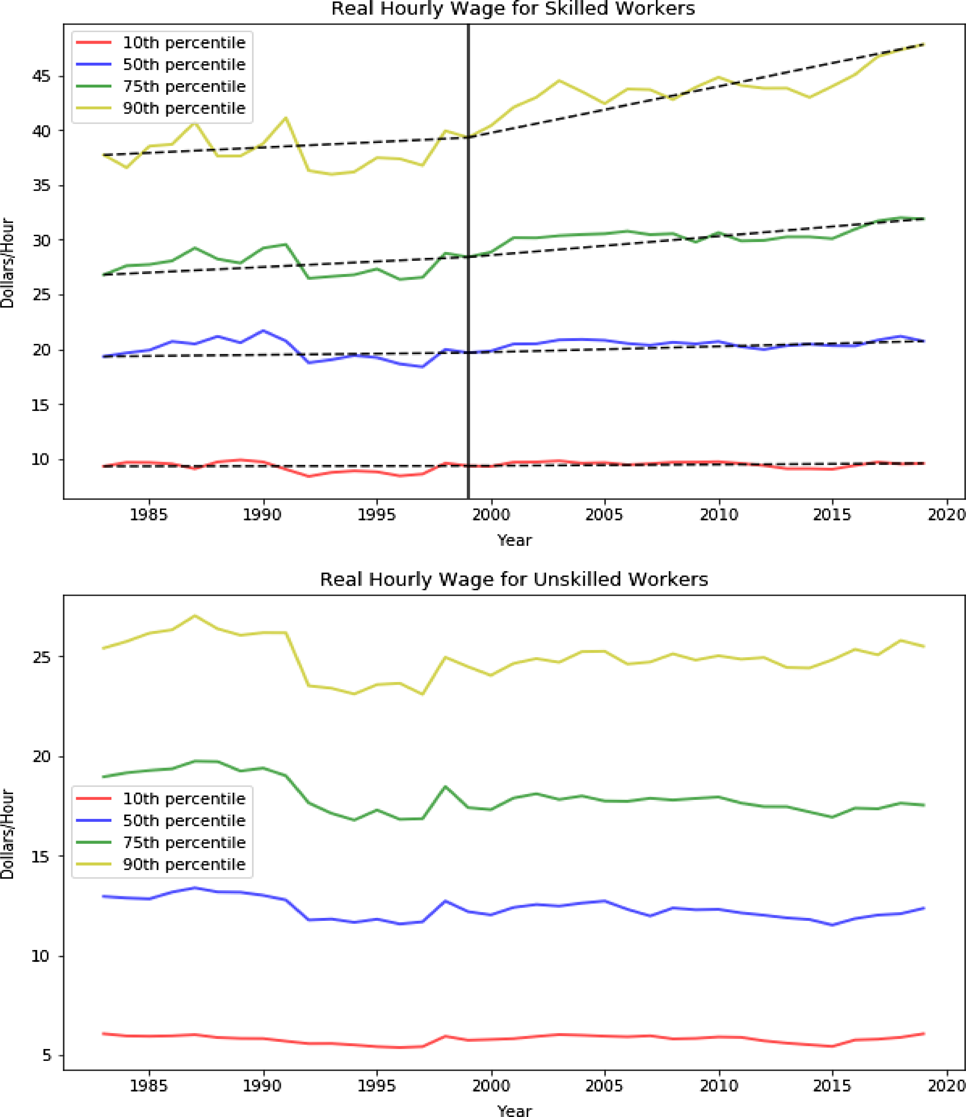
Figure 1. Real hourly wage for silled and unskilled workers.
Note: Calculation based on CPS ASEC data, 1983–2019. Both panels show various percentiles of the real hourly wage for workers with (skilled) or without (unskilled) a bachelor’s degree. Real hourly wages are calculated using annual wage and salary divided by usual hours worked per year. I adjust for inflation using Consumer Price Index adjustment factors which convert dollar amounts to constant 1999 dollars (CPI99 in IPUMS), so all values are expressed as 1999 dollars. The sample comprises nonfarm wage and salary workers who are 25–64 years old. The dotted lines in the top panel give the slope of wage growth during periods before and after 1999 (vertical line).
First and foremost, the trend of wage growth for skilled workers varies a lot across percentile groups before and after 2000. To be specific, as shown in the top panel of Fig. 1, the growth rate of real wages for above-median college degree holders significantly accelerated around 2000 relative to their lower-tail peers. Table 1 reemphasizes the point by confirming that the gaps in real wage growth between percentiles were not large during 1983–1999 but were substantially widened afterward. For example, one can find in particular that the real wage growth of the top 10th percentile of skilled workers significantly accelerated starting from 2000 compared to their peers, as reflected by the larger difference between the average annual growth before and after 2000. However, the divergence is not present for the group of unskilled workers, within which the growth rates of wages are relatively invariant across percentile groups. This observation is consistent with the finding in Autor et al. (Reference Aghion and Kearney2008) that the bulk of within-group inequality occurs above the median of the wage distribution in recent decades, given that presumably college degree holders represent the upper tail of the wage distribution. One subtle difference of my observation from what they found is essentially the notable acceleration of divergence within the educated group rather than the whole population after 2000.
Second, despite the sharp increase in the college wage premium, the bottom half of skilled workers barely benefited from it. Table 1 makes it clear that the growth of real wage for the first decile of college degree holders was almost zero in the past four decades, and it is probably surprising to note that even the median college degree holders experienced negligible real wage increase compared to their upper-tail peers. This observation, combined with the last one, suggests that in contrast to the conventional view that the increase in the college wage premium benefits most of the college degree holders, it is just the top half of them that benefits. Thus, wage dispersion has been increasingly enlarged since the beginning of the 21st century.
Table 1. Annual % change in real wage
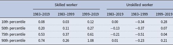
Note: Annual % change is calculated by the cumulative % change over the corresponding period divided by the number of years.
Lastly, unskilled workers saw a mild decline in real wages in the recent 40 years. Although there is a general agreement on this fact in many works based on various sources of dataset,Footnote 8 the fact is still relevant and noteworthy in the context of wage inequality because it serves as a natural contrast to the first fact related to within-group inequality. The divergence of wage growth across percentile groups that is salient for the skilled group is not present for the unskilled group at all, which indicates a tied connection between the widening of within-group wage inequality and the specific group of skilled workers.
2.2. Empirical implementation
In this section, I implement an empirical strategy to quantify the magnitude of the change in the trend of wage inequality as observed. Besides, using the task-based framework by ALM, I run the same regression for the subsamples of workers in five occupations to explore which occupations drive the changing trend. One remarkable finding is that the changing trend of wage inequality was entirely driven by one category of task, namely the nonroutine analytic task.
The occupations based on consistent three-digit COC in CPS data are classified as five categories of task groups following the criterion in ALM and David and Dorn (Reference David and Dorn2013). They are nonroutine analytic, nonroutine interactive, routine cognitive, routine manual, and nonroutine manual tasks. They are constructed using the rank of certain measures of task intensity by the Dictionary of Occupational Titles (DOT). Occupations with the highest rank among five measures of task intensity are attributed to corresponding categories.Footnote 9
I then run the following regression for skilled workers as well as the subsamples of workers in each of the five occupations defined above:
 \begin{equation} WI^{i} = \beta _{0}^{i} + \beta _{1}^{i} \, Year + \beta _{2}^{i} \, \unicode{x1D7D9} (Post2000) + \beta _{3}^{i} \, \unicode{x1D7D9} (Post2000) \times Year + \epsilon ^{i} \end{equation}
where $i$
denotes different (sub) groups of workers and
$i$
denotes different (sub) groups of workers and $WI^{i}$
is a set of measures of wage differentials for the whole group and five subgroups obtained by taking log differences between wage percentiles in each group;
$WI^{i}$
is a set of measures of wage differentials for the whole group and five subgroups obtained by taking log differences between wage percentiles in each group; $Year$
captures the time trend of wage differential; and
$Year$
captures the time trend of wage differential; and $\unicode{x1D7D9} (Post2000)$
is an indicator of whether the observation is on or after 2000 (1 if it is and 0 otherwise). Therefore, the coefficients of interest are
$\unicode{x1D7D9} (Post2000)$
is an indicator of whether the observation is on or after 2000 (1 if it is and 0 otherwise). Therefore, the coefficients of interest are $\beta _{2}^{i}$
and
$\beta _{2}^{i}$
and $\beta _{3}^{i}$
, which reflect the magnitude of the shift in wage inequality and the change of the slopes (trend) after 2000 separately.
$\beta _{3}^{i}$
, which reflect the magnitude of the shift in wage inequality and the change of the slopes (trend) after 2000 separately.
The results shown in the first column of Table 2 confirm the observation that the top 10% of skilled workers gained greatly over their peers after 2000. For example, the growth of the 90/10 percentile differential widens about 0.4% per year on average after 2000 relative to before. This is a sizable change of wage structure because on average, the differential grows about 0.2% each year ( $\beta _{1}$
), which means the magnitude of the widening amounts to two times the previous trend of the growth of wage differential. In some cases, this change of trend is augmented with a one-time upward shift after 2000. Other measures of upper-tail wage inequality also significantly increased after 2000, while measures of lower-tail wage inequality (50–10) did not.
$\beta _{1}$
), which means the magnitude of the widening amounts to two times the previous trend of the growth of wage differential. In some cases, this change of trend is augmented with a one-time upward shift after 2000. Other measures of upper-tail wage inequality also significantly increased after 2000, while measures of lower-tail wage inequality (50–10) did not.
Table 2. Changes in wage inequality after 2000
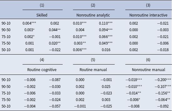
Note: This table displays the results of the regression (equation (1)) for the whole sample of skilled workers (column 1), as well as the subsamples of workers in the five occupations (columns (2)–(6)). The values on the left and right in each column are estimates of $\beta _{3}$
and
$\beta _{3}$
and $\beta _{2}$
separately. ***, **, and * indicate the estimator is significant at 1%, 5%, and 10% level.
$\beta _{2}$
separately. ***, **, and * indicate the estimator is significant at 1%, 5%, and 10% level.
I then investigate which category of occupation (task) drives the changing trend of wage inequality for the overall skilled workers by implementing the same regression for the five subgroups of workers defined above, from which we might have a sense of what kinds of skilled workers gained more after 2000 and why. Interestingly, the classification of occupation under the task-based framework shows an informative picture of differential behaviors of wage inequality across occupation categories, although the interpretation is slightly different from ALM which focuses only on the reallocation of task input demand rather than wage inequality.
The results in columns (2)–(6) demonstrate it is essentially just one occupation (task) that contributes to the increases in the growth of overall within-group inequality, namely the nonroutine analytic task. It is appealing to find that the nonroutine analytic task not only underwent a widening of upper-tail wage inequality in trend after 2000, but also the magnitude was more than twice as much compared to the whole skilled group. The change of trend (slope) was also augmented with a sizable one-time upward shift. In contrast, none of the rest of the occupations showed a significant shift in the trend of the wage structure after 2000. If any, there was a notable contraction of wage inequality for the nonroutine manual jobs. Put together, the evidence suggests that the change of the trend of upper-tail wage differential within the skilled group is exclusively driven by that within nonroutine analytic jobs, which also more than offset the opposite force brought about by the contraction of wage inequality within nonroutine manual jobs.
2.3. Educational distribution
Because my empirical analysis mainly focuses on wage inequality within skilled workers who have at least a bachelor’s degree, I am interested in to what extent does this relate to the overall inequality. It turns out the answer that greatly depends on which category of occupation we are looking at. I also investigate which occupations employ the most workers with college degrees. Understanding those helps shed a light on what might drive the changing structure of wage inequality within the skilled group.
One appealing finding is that the bulk of workers consists of skilled workers in the analytic task, which is exactly the task that underwent a changing trend of wage inequality. This suggests a close link between the skill intensity of a task and its structure of wage inequality. Fig. 2 shows a clear hierarchical pattern of the share of skilled workers for the five occupation categories. More than half of the workers doing nonroutine analytic jobs are college degree holder, and the task skill intensity is kept increasing in the recent four decades. For nonroutine interactive jobs, this number is a bit lower. For the rest of the three categories, the skill intensity is greatly lower, although routine manual jobs are well above the other two.
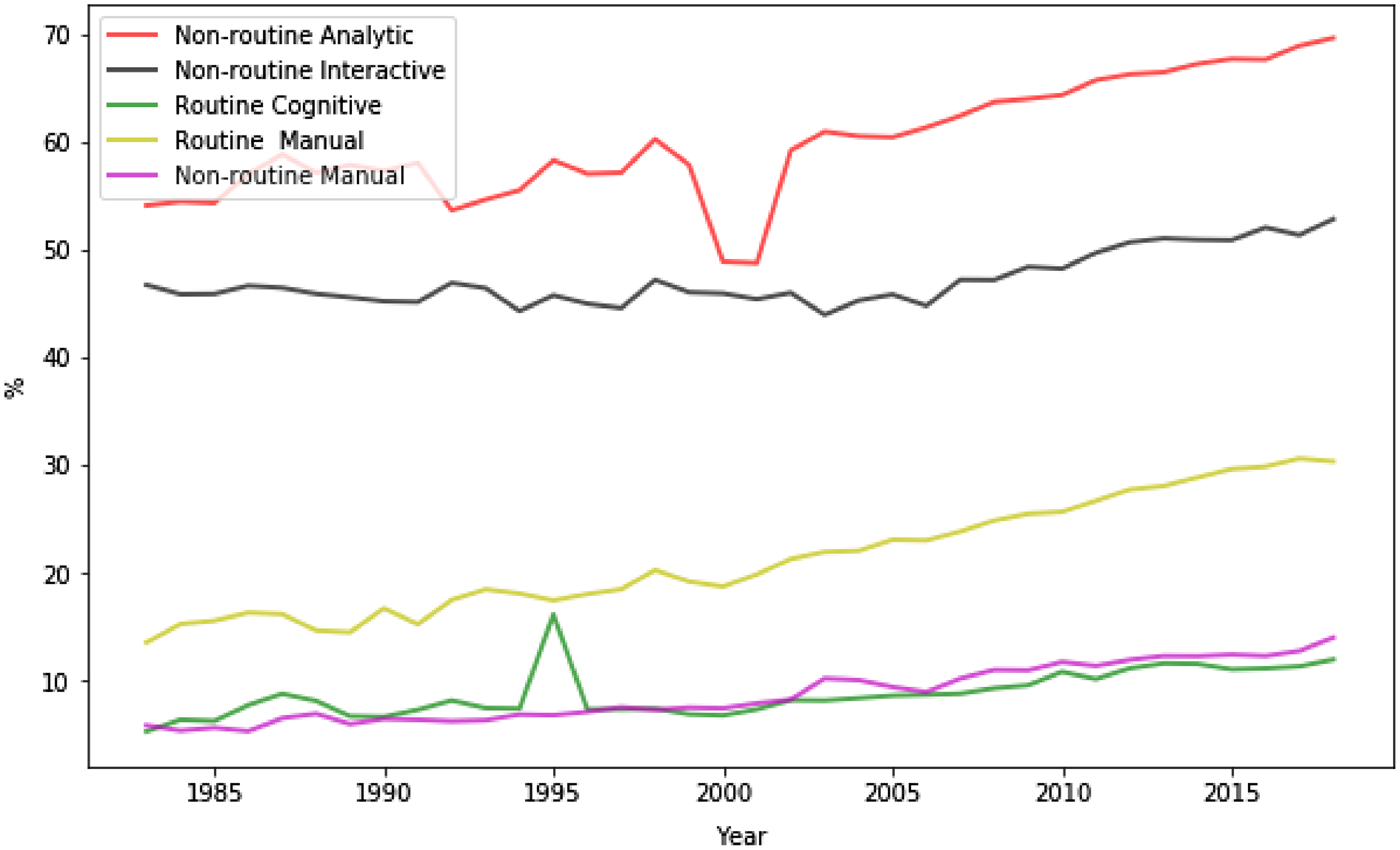
Figure 2. Percentage of college degree holder.
Note: The values are shares of workers with at least a bachelor’s degree in each category of occupation.

Figure 3. Destinations of college degree holders.
Note: The values show what percentage of skilled workers (with at least a bachelor’s degree) goes to each category of occupation, so the five numbers in each year add up to one.
The data on the destinations of skilled workers convey a similar big picture as Fig. 2 with slightly more information. Fig. 3 explores the educational distribution from the other direction, which is what percentage of skilled workers goes to the five categories of occupations separately. It shows most (more than 80%) of the college degree holders work in nonroutine cognitive occupations. It is notably interesting that the percentage of skilled workers working in nonroutine analytic jobs surpassed interactive jobs just around 2000, coinciding with the timing of the change of the wage structure within nonroutine cognitive jobs.Footnote 10
3. A model of task reallocation and wage inequality
To interpret the empirical evidence that the trend of wage dispersion became steeper and the changing trend was entirely driven by the nonroutine analytic task, one starting point is the standard implications of the task-based framework as in ALM, which suggest a composition effect as the main driving force of the change of wage structure. The idea is that machines are more likely to substitute labor in the routine task, then when the price of capital (investment) drops, labor in the routine task will be replaced by machines and crowded out to other tasks.Footnote 11 Since workers are heterogeneous in task-specific labor efficiencies, the reallocation of labor will result in a changing composition of workers and affect the demand and supply of labor within each task.
In this section, I investigate how the composition effect would affect within-group wage inequality and whether it could broadly fit into the empirical evidence by developing a discrete time general equilibrium model building on vom Lehn (Reference vom Lehn2020) that features labor reallocation across tasks. Instead of three task inputs (abstract, routine, and manual) in his work, I consider only two tasks: abstract and routine. One can understand the abstract task as a model counterpart of the nonroutine analytic task defined in Section 2 and the routine task as a composite of the rest of the tasks. In this model, workers are heterogeneous in one dimension, namely the amount of labor efficiency in the abstract task, and the task reallocation is driven by the substitution of labor in the routine task by machines embodied by capital. The capital stock accumulates because of ongoing investment-specific technical change, as emphasized in the work of Greenwood et al. (Reference Greenwood, Hercowitz and Krusell1997).Footnote 12 The goal of abstracting from more task inputs and using the simplest possible framework is to focus on the implications of wage inequality in the nonroutine analytic task when it is linked to the task reallocation model. This is the main theoretical innovation and contribution of the paper. A richer model could be developed later to better explain the empirical facts we found in the last section.
3.1. Environment: firms and production
There is a representative firm operating a production technology for the final output. The production function is a standard nested CES production function using two task inputs—abstract and routine task:
 \begin{equation} Y_{t} = [\mu _{a} N_{at}^{\frac{\gamma _{a} - 1}{\gamma _{a}}} + (1 - \mu _{a}) [(1 - \mu _{r}) K_{t}^{\frac{\gamma _{r} - 1}{\gamma _{r}}} + \mu _{r} N_{rt}^{\frac{\gamma _{r} - 1}{\gamma _{r}}}]^{\frac{\gamma _{r} (\gamma _{a} - 1)}{\gamma _{a}(\gamma _{r} - 1)}}]^{\frac{\gamma _{a}}{\gamma _{a} - 1}} \end{equation}
where the subscript $a$
(
$a$
( $r$
) refers to the abstract (routine) task,
$r$
) refers to the abstract (routine) task, $N_{at}$
(
$N_{at}$
( $N_{rt}$
) is efficiency units of labor in the abstract (routine) task, and
$N_{rt}$
) is efficiency units of labor in the abstract (routine) task, and $K_{t}$
is machines embodied by capital. The parameters include
$K_{t}$
is machines embodied by capital. The parameters include $\gamma _{a}$
(
$\gamma _{a}$
( $\gamma _{r}$
), which is the corresponding elasticity of substitution between routine and abstract tasks (routine labor and machines), and
$\gamma _{r}$
), which is the corresponding elasticity of substitution between routine and abstract tasks (routine labor and machines), and $\mu _{a}$
(
$\mu _{a}$
( $\mu _{r}$
), which is the relative weight of the abstract (routine) labor in production. The terms in the first square bracket indicate that the output of the abstract task is produced simply using the total efficiency units of labor in that task, while for the routine task, the output could be produced by either machines
$\mu _{r}$
), which is the relative weight of the abstract (routine) labor in production. The terms in the first square bracket indicate that the output of the abstract task is produced simply using the total efficiency units of labor in that task, while for the routine task, the output could be produced by either machines $K$
or labor. That investment-specific technological change can potentially substitute for routine labor and is the key mechanism of shifts in employment across tasks to capture the fundamental task replacement arguments put forth by ALM.
$K$
or labor. That investment-specific technological change can potentially substitute for routine labor and is the key mechanism of shifts in employment across tasks to capture the fundamental task replacement arguments put forth by ALM.
The problem for the firm is
 \begin{equation} \max _{K_{t},N_{rt},N_{at}} Y_{t} - r_{t} K_{t} - w_{rt} N_{rt} - w_{at} N_{at} \end{equation}
3.2. Environment: workers
To simplify the household problem, I assume a representative family setup, in which the household owns the capital and is comprised of a continuum of workers of measure one. Each worker supplies one unit of labor inelastically. For Preferences, I assume a standard logarithmic specification for households’ instantaneous utility with discount factor $\beta$
:
$\beta$
:
 \begin{equation} u(c) = \log\!(c_{t}) \end{equation}
The household accumulates capital by the following law of motion:
 \begin{equation} K_{t+1} = (1-\delta )K_{t} +q_{t}I_{t} \end{equation}
where $q_{t}$
is the relative price of consumption to investment goods and included in the equation of capital evolution following Greenwood et al. (Reference Greenwood, Hercowitz and Krusell1997).Footnote 13 An increase in
$q_{t}$
is the relative price of consumption to investment goods and included in the equation of capital evolution following Greenwood et al. (Reference Greenwood, Hercowitz and Krusell1997).Footnote 13 An increase in $q_{t}$
represents increased investment-specific technological progress and is the main driving force of the model. Its movement is assumed to be exogenously determined for now.
$q_{t}$
represents increased investment-specific technological progress and is the main driving force of the model. Its movement is assumed to be exogenously determined for now.
In addition, workers are heterogeneous in efficiency units of labor in the abstract task, which is represented by a single index $z$
. This assumption is key in generating a dispersed wage distribution in the abstract task that can be mapped back to the data and evaluated quantitatively. I assume that the distribution of
$z$
. This assumption is key in generating a dispersed wage distribution in the abstract task that can be mapped back to the data and evaluated quantitatively. I assume that the distribution of $z$
is simply standard normal. A worker with
$z$
is simply standard normal. A worker with $z$
provides
$z$
provides $\phi _{a}(z)$
efficiency units of labor in the production of abstract task, where
$\phi _{a}(z)$
efficiency units of labor in the production of abstract task, where $\phi _{a}(z) = e^{\alpha _{a}z}$
, so that the distribution of efficiency units is log-normal. Therefore, wages for a worker with skill level
$\phi _{a}(z) = e^{\alpha _{a}z}$
, so that the distribution of efficiency units is log-normal. Therefore, wages for a worker with skill level $z$
in the abstract occupation are given by the product of the common skill price,
$z$
in the abstract occupation are given by the product of the common skill price, $w_{at}$
, and the heterogeneous efficiency units in the abstract occupation,
$w_{at}$
, and the heterogeneous efficiency units in the abstract occupation, $\phi _{a}(z)$
. For simplicity, I assume that the abstract skill level does not affect workers’ productivity in the routine task (
$\phi _{a}(z)$
. For simplicity, I assume that the abstract skill level does not affect workers’ productivity in the routine task ( $\phi _{r}(z) = 1$
), so wages in that task are homogeneous. Abstracting from the heterogeneity of workers in the routine task simplifies the structure but will not affect the main focus of the model .
$\phi _{r}(z) = 1$
), so wages in that task are homogeneous. Abstracting from the heterogeneity of workers in the routine task simplifies the structure but will not affect the main focus of the model .
Thus, the representative household problem is given by:
 \begin{equation} \max _{C_{t}(z),O_{t}(z),K_{t+1}} \sum _{t=0}^{\infty } \beta ^{t}\int _{z} \log\!(C_{t}(z)) d\Phi (z) \end{equation}
 \begin{equation*} s.t. \quad C_{t} + I_{t} = r_{t} K_{t} + \int _{z} W_{t}(z) d\Phi (z) \quad {\rm and} \quad K_{t+1} = (1-\delta )K_{t} +q_{t}I_{t} \end{equation*}
where $K_{t}$
is the household’s total capital holdings,
$K_{t}$
is the household’s total capital holdings, $O_{t}(z)$
is the occupational choice (abstract or routine task) for each individual, and
$O_{t}(z)$
is the occupational choice (abstract or routine task) for each individual, and $W_{t}(z)$
, the wage for an individual with
$W_{t}(z)$
, the wage for an individual with $z$
, is obtained by
$z$
, is obtained by $\sum _{j} \unicode{x1D7D9}(O_{t}(z)=j) w_{jt}\phi _{j}(z)$
.
$\sum _{j} \unicode{x1D7D9}(O_{t}(z)=j) w_{jt}\phi _{j}(z)$
.
The representative family setup implies that consumption will be equalized across all workers, which greatly simplifies the model. Since consumption inequality and its labor market implications are not the main focus here, this parsimonious framework would not affect the central point of interest, which is wage inequality.
3.3. Definition of equilibrium
The competitive equilibrium for the economy consists of a set of prices ( $r_{t}, w_{at}, w_{mt}$
) and allocations (
$r_{t}, w_{at}, w_{mt}$
) and allocations ( $C_{t}(z),O_{t}(z)$
,
$C_{t}(z),O_{t}(z)$
, $K_{t},N_{rt},N_{at}$
), such that:
$K_{t},N_{rt},N_{at}$
), such that:
-
(1) Taking prices ( $r_{t}, w_{at}, w_{mt}$
) as given, workers choose (
$C_{t}(z),O_{t}(z),K_{t+1}$
) to solve (6) starting from any initial conditions
$K_{0}$
for all
$t \geq 1$
$r_{t}, w_{at}, w_{mt}$
) as given, workers choose (
$C_{t}(z),O_{t}(z),K_{t+1}$
) to solve (6) starting from any initial conditions
$K_{0}$
for all
$t \geq 1$
-
(2) Taking (
$r_{t}, w_{at}, w_{mt}$
) as given, the firm chooses (
$K_{t},N_{rt},N_{at}$
) to solve (2); -
(3) Labor and output markets clear:
(7)and resource constraint:
\begin{equation} N_{jt} = \int _{z} \unicode{x1D7D9}(O_{t}(z)=j) \phi _{j}(z) d\Phi (z) \qquad j = a,r \end{equation}
(8)
\begin{equation} Y_{t} = C_{t} + I_{t} = C_{t} + \frac{1}{q_{t}}(K_{t+1} - (1-\delta )K_{t}) \end{equation}


3.4. Characterization of equilibrium
Since the full path of $q_{t}$
is deterministic and its movement is the primary driving force for the incentives of investment, it is useful to relate the rental rate of capital
$q_{t}$
is deterministic and its movement is the primary driving force for the incentives of investment, it is useful to relate the rental rate of capital $r_{t}$
to
$r_{t}$
to $q_{t}$
. Therefore, it is convenient to rewrite the Euler equation for the model in the following way:
$q_{t}$
. Therefore, it is convenient to rewrite the Euler equation for the model in the following way:
 \begin{equation} r_{t+1} = \frac{1}{q_{t}}\!\left(\frac{C_{t+1}}{\beta C_{t}} - \frac{1-\delta }{\frac{q_{t+1}}{q_{t}}}\right) \end{equation}
A worker’s problem can then be characterized by the Euler equation (9). Note that the rental rate of capital next period $r_{t+1}$
is not only a decreasing function of
$r_{t+1}$
is not only a decreasing function of $q_{t}$
but also an increasing function of the growth rate of
$q_{t}$
but also an increasing function of the growth rate of $q$
. The first result holds simply because an increase in
$q$
. The first result holds simply because an increase in $q_{t}$
leads to higher investment and thus induces a higher supply of capital in this period, which has a downward pressure on the rental rate next period. The growth rate of
$q_{t}$
leads to higher investment and thus induces a higher supply of capital in this period, which has a downward pressure on the rental rate next period. The growth rate of $q_{t}$
also affects the rental rate as a high growth rate will lower the relative capital gains on undepreciated capital and thus offsets declines in the rental rate.
$q_{t}$
also affects the rental rate as a high growth rate will lower the relative capital gains on undepreciated capital and thus offsets declines in the rental rate.
Then, I characterize the assignment of workers into tasks based on a comparative advantage structure. The main feature of the equilibrium is that the assignment of labor takes a form of the threshold value. Formally, there exists a unique $z^{*}$
such that workers with
$z^{*}$
such that workers with $z \gt z^{*}$
choose to work in the abstract task, while workers with
$z \gt z^{*}$
choose to work in the abstract task, while workers with $z \lt z^{*}$
choose to work in the routine task.Footnote 14
$z \lt z^{*}$
choose to work in the routine task.Footnote 14
The key driving force of the model is that as a technical change takes place, the prices for investment goods drop ( $q$
increases). Cheaper investment goods induce the firm to replace the labor in the routine task by machines. Workers who become obsolete in the routine task have to relocate to the abstract task. From the threshold argument above, we know that the marginal entrants to the abstract task are lower types of
$q$
increases). Cheaper investment goods induce the firm to replace the labor in the routine task by machines. Workers who become obsolete in the routine task have to relocate to the abstract task. From the threshold argument above, we know that the marginal entrants to the abstract task are lower types of $z$
compared to the incumbents. This drives the threshold value
$z$
compared to the incumbents. This drives the threshold value $z^{*}$
down and changes the composition of the workers in terms of
$z^{*}$
down and changes the composition of the workers in terms of $z$
in the abstract task. This mechanism of labor assignment and mobility based on comparative advantage is closely related to the classic work by Roy (Reference Roy1951) and many modern treatments of the Roy model.Footnote
15
$z$
in the abstract task. This mechanism of labor assignment and mobility based on comparative advantage is closely related to the classic work by Roy (Reference Roy1951) and many modern treatments of the Roy model.Footnote
15
Finally, the prices ( $r_{t}$
,
$r_{t}$
, $w_{at}$
,
$w_{at}$
, $w_{mt}$
) can be obtained in terms of aggregate variables using the first-order conditions by the firm’s profit maximization problem (3):
$w_{mt}$
) can be obtained in terms of aggregate variables using the first-order conditions by the firm’s profit maximization problem (3):
 \begin{equation} w_{at} = \mu _{a}\!\left(\frac{Y_{t}}{N_{at}}\right)^{\frac{1}{\gamma _{a}}} \end{equation}
 \begin{equation} w_{rt}= (1-\mu _{a})\mu _{r}Y_{t}^{\frac{1}{\gamma _{a}}}R_{t}^{\frac{\gamma _{a}-\gamma _{r}}{\gamma _{a}(\gamma _{r}-1)}}\!\left(\frac{1}{N_{rt}}\right)^{\frac{1}{\gamma _{r}}} \end{equation}
 \begin{equation} r_{t}= (1-\mu _{a})(1-\mu _{r})Y_{t}^{\frac{1}{\gamma _{a}}}R_{t}^{\frac{\gamma _{a}-\gamma _{r}}{\gamma _{a}(\gamma _{r}-1)}}\!\left(\frac{1}{K_{t}}\right)^{\frac{1}{\gamma _{r}}} \end{equation}
4. Model solution and calibration
This section links the model to the data by constructing the path of the sole exogenous driving force of the model, $q_{t}$
. In this section, I describe the measurement of
$q_{t}$
. In this section, I describe the measurement of $q_{t}$
, the calibration of all model parameters, with which I briefly discuss how the model can be solved.
$q_{t}$
, the calibration of all model parameters, with which I briefly discuss how the model can be solved.
4.1. Exogenous forcing process and model solution
To solve and evaluate the model quantitatively, I construct the entire path of $q_{t}$
following vom Lehn (Reference vom Lehn2020), which used the deflator for investment goods as constructed following Gordon (Reference Gordon1990). As in Greenwood et al. (Reference Greenwood, Hercowitz and Krusell1997),
$q_{t}$
following vom Lehn (Reference vom Lehn2020), which used the deflator for investment goods as constructed following Gordon (Reference Gordon1990). As in Greenwood et al. (Reference Greenwood, Hercowitz and Krusell1997), $q_{t}$
is measured as the price of consumption divided by the price of equipment and software investment. I assume that the time series starts in a steady state with
$q_{t}$
is measured as the price of consumption divided by the price of equipment and software investment. I assume that the time series starts in a steady state with $q_{1}$
normalized to 1 in the year 1983. The data are available until 2015, after which I assume the growth rate of
$q_{1}$
normalized to 1 in the year 1983. The data are available until 2015, after which I assume the growth rate of $q_{t}$
linearly decays to zero in a few years.Footnote 16 The entire path of
$q_{t}$
linearly decays to zero in a few years.Footnote 16 The entire path of $q_{t}$
and its growth is plotted in Fig. 4.
$q_{t}$
and its growth is plotted in Fig. 4.
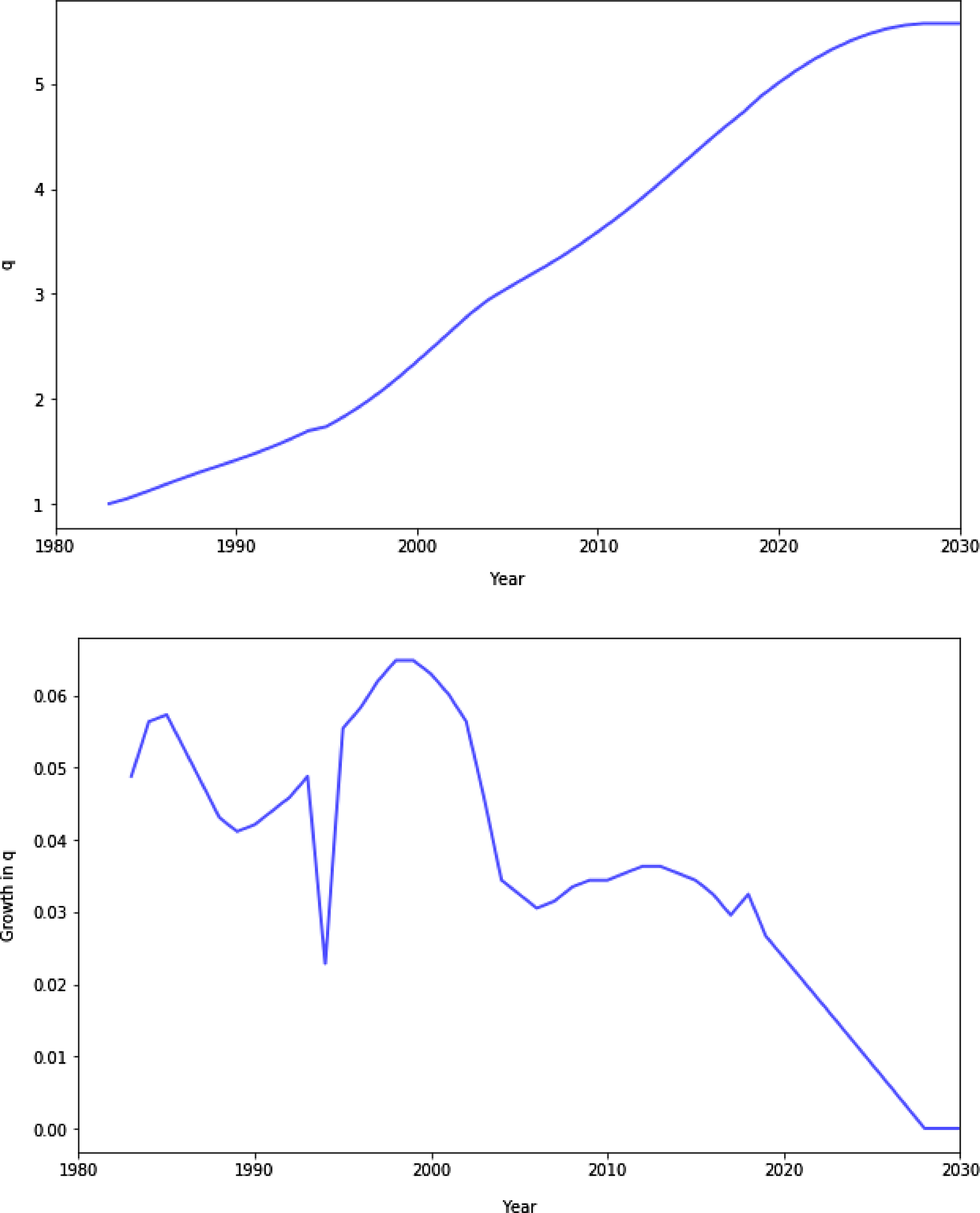
Figure 4. Time path and growth rate of $q_{t}$
.
$q_{t}$
.
Note: The time series starts in a steady state with $q_{1}$
normalized to 1. The data of
$q_{1}$
normalized to 1. The data of $q_{t}$
calculated based on the price index of investment goods constructed in Gordon (Reference Gordon1990) is available until 2015, after which it is assumed that the growth rate of
$q_{t}$
calculated based on the price index of investment goods constructed in Gordon (Reference Gordon1990) is available until 2015, after which it is assumed that the growth rate of $q_{t}$
linearly decays to zero in 12 years. The growth of
$q_{t}$
linearly decays to zero in 12 years. The growth of $q$
in period
$q$
in period $t$
is given by
$t$
is given by $\log\!(q_{t+1}) - \log\!(q_{t})$
.
$\log\!(q_{t+1}) - \log\!(q_{t})$
.
With the values of $q_{t}$
, I can first obtain any steady state variables using the Euler equation (9). I then calibrate the parameters of the model so that the model solution matches certain empirical counterparts. Lastly, the transition path is solved using a standard shooting algorithm given that we know the initial and terminal steady states. The details of solving the model are in Section 5 and Appendix A.
$q_{t}$
, I can first obtain any steady state variables using the Euler equation (9). I then calibrate the parameters of the model so that the model solution matches certain empirical counterparts. Lastly, the transition path is solved using a standard shooting algorithm given that we know the initial and terminal steady states. The details of solving the model are in Section 5 and Appendix A.
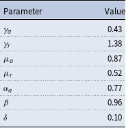
4.2. Calibration
The parameters to calibrate are the elasticities of substitution ( $\gamma _{a}$
,
$\gamma _{a}$
, $\gamma _{r}$
), share parameters in the production function (
$\gamma _{r}$
), share parameters in the production function ( $\mu _{a}$
,
$\mu _{a}$
, $\mu _{r}$
), the scaling parameter of productivity function in the abstract task (
$\mu _{r}$
), the scaling parameter of productivity function in the abstract task ( $\alpha _{a}$
), capital depreciation rate (
$\alpha _{a}$
), capital depreciation rate ( $\delta$
), and discount factor (
$\delta$
), and discount factor ( $\beta$
). Among those parameters, the discount factor and depreciation rates can be set externally following a standard value as estimated in Cummins and Violante (Reference Cummins and Violante2002). This gives
$\beta$
). Among those parameters, the discount factor and depreciation rates can be set externally following a standard value as estimated in Cummins and Violante (Reference Cummins and Violante2002). This gives $\beta = 0.96$
and
$\beta = 0.96$
and $\delta = 0.1$
. Besides, since the structure of production is almost identical to the one in vom Lehn (Reference vom Lehn2020), except that manual jobs are aggregated in the routine task, I use his calibration results for the elasticities of substitution. So we have
$\delta = 0.1$
. Besides, since the structure of production is almost identical to the one in vom Lehn (Reference vom Lehn2020), except that manual jobs are aggregated in the routine task, I use his calibration results for the elasticities of substitution. So we have $\gamma _{a} = 0.43$
and
$\gamma _{a} = 0.43$
and $\gamma _{r} = 1.38$
.
$\gamma _{r} = 1.38$
. $\gamma _{r} \gt 1 \gt \gamma _{a}$
implies that capital is a substitute for the labor input in the routine task, while the routine task and abstract task are a gross complement. The values of elasticities capture the key qualitative attributes of tasks that are necessary for the desired task reallocation and are therefore reasonable results for calibration.
$\gamma _{r} \gt 1 \gt \gamma _{a}$
implies that capital is a substitute for the labor input in the routine task, while the routine task and abstract task are a gross complement. The values of elasticities capture the key qualitative attributes of tasks that are necessary for the desired task reallocation and are therefore reasonable results for calibration.
I calibrate the share parameters in the production function ( $\mu _{a}$
,
$\mu _{a}$
, $\mu _{r}$
) in the way that the labor share of output and the fraction of labor income in routine and abstract jobs in the initial steady state match their empirical counterparts in 1983.
$\mu _{r}$
) in the way that the labor share of output and the fraction of labor income in routine and abstract jobs in the initial steady state match their empirical counterparts in 1983. $\alpha _{a}$
is calibrated such that the log difference between the 90th percentile and 10th percentile of the wage is matched to the data in 1983. Table 3 summarizes parameter values for the calibration.
$\alpha _{a}$
is calibrated such that the log difference between the 90th percentile and 10th percentile of the wage is matched to the data in 1983. Table 3 summarizes parameter values for the calibration.
Table 3. Calibrated values for model parameters
Note: This table reports the values for calibrated model parameters. They are elasticities of substitution ( $\gamma _{a}$
,
$\gamma _{a}$
, $\gamma _{r}$
), share parameters in the production function (
$\gamma _{r}$
), share parameters in the production function ( $\mu _{a}$
,
$\mu _{a}$
, $\mu _{r}$
), the scaling parameter of productivity function in the abstract task (
$\mu _{r}$
), the scaling parameter of productivity function in the abstract task ( $\alpha _{a}$
), capital depreciation rate (
$\alpha _{a}$
), capital depreciation rate ( $\delta$
), and discount factor (
$\delta$
), and discount factor ( $\beta$
).
$\beta$
).
5. Results
In this section, I present results to the model solution by showing how the steady states and transition dynamics would evolve when $q$
changes exogenously. The results not only establish the intuition that labor in the routine task will relocate to the abstract task when an ongoing investment-specific technical change takes place, and wage inequality in the abstract task widens as a result of the composition effect, but also remarkably predict a nonlinear expansion path of wage dispersion in the abstract task which is comparable to the empirical evidence. The last subsection discusses why such a parsimonious framework could generate the desired transition path.
$q$
changes exogenously. The results not only establish the intuition that labor in the routine task will relocate to the abstract task when an ongoing investment-specific technical change takes place, and wage inequality in the abstract task widens as a result of the composition effect, but also remarkably predict a nonlinear expansion path of wage dispersion in the abstract task which is comparable to the empirical evidence. The last subsection discusses why such a parsimonious framework could generate the desired transition path.
5.1. Steady states
Before showing the full solution to the model, I provide a rough idea of how the movement of $q_{t}$
could shape wage inequality by presenting the solution of the model for two steady states and characterize the implications for wage inequality. The two steady states are initial steady state, in which
$q_{t}$
could shape wage inequality by presenting the solution of the model for two steady states and characterize the implications for wage inequality. The two steady states are initial steady state, in which $q$
is normalized to 1 and is already in a steady state, and terminal steady state, in which
$q$
is normalized to 1 and is already in a steady state, and terminal steady state, in which $q$
is equal to its terminal value
$q$
is equal to its terminal value $q_T$
and stays there afterward.
$q_T$
and stays there afterward.
All steady state variables can be easily obtained by utilizing properties of truncated log-normal distribution and solving equations (9)–(12) in closed form.Footnote
17
The results of two steady states with $q_{1} = 1$
and
$q_{1} = 1$
and $q_{T} = 5.6$
are displayed in Table 4.
$q_{T} = 5.6$
are displayed in Table 4.
Table 4. Comparison of steady state variables
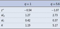
Note: Values are for initial and terminal steady states separately. $z^{*}$
,
$z^{*}$
, $\bar{w_{a}}$
,
$\bar{w_{a}}$
, $\bar{w_{r}}$
, and
$\bar{w_{r}}$
, and $K$
represent the threshold value of
$K$
represent the threshold value of $z$
, average wages for abstract and routine tasks, and capital stock, respectively.
$z$
, average wages for abstract and routine tasks, and capital stock, respectively.
Before looking directly at the implications of investment-specific technical change and task reallocation for wage inequality, we can see that the results suggest one obvious mechanism that would affect wage inequality within the abstract task, namely the composition effect, which results from the reallocation of labor with low $z$
from the routine task to the abstract task. This could be made clear by the different threshold values of
$z$
from the routine task to the abstract task. This could be made clear by the different threshold values of $z^{*}$
in two steady states as shown in the first row of Table 4. The transition of the economy induced by increased investment-specific technical change features departing from a high level of
$z^{*}$
in two steady states as shown in the first row of Table 4. The transition of the economy induced by increased investment-specific technical change features departing from a high level of $z^{*}$
to a low level, which implies more workers in the abstract task and fewer workers in the routine task. This is because increases in
$z^{*}$
to a low level, which implies more workers in the abstract task and fewer workers in the routine task. This is because increases in $q$
stimulate a higher investment level and capital stock, which replaces the labor in the routine task. As a result, an increasing amount of labor in the routine task relocates to the abstract task, and since the marginal entrants are lower types of
$q$
stimulate a higher investment level and capital stock, which replaces the labor in the routine task. As a result, an increasing amount of labor in the routine task relocates to the abstract task, and since the marginal entrants are lower types of $z$
compared to the incumbents, the range of
$z$
compared to the incumbents, the range of $z$
in the abstract task is expanded and the wage inequality could be mechanically widened due to the composition effect.
$z$
in the abstract task is expanded and the wage inequality could be mechanically widened due to the composition effect.
As shown in the second row of the table, there should be a price effect because the transition of the economy is also accompanied by an increase in the wage rate in the abstract task.Footnote
18
Since the total wage of a worker is the product of wage rate and efficiency units, the increase of wage rate amplifies the variance of total wage within the abstract task holding the distribution of $z$
fixed. However, since we focus on the relative change of wage inequality within the abstract task throughout the transition path, this price effect would drop out and not affect the measure of (relative) wage inequality.
$z$
fixed. However, since we focus on the relative change of wage inequality within the abstract task throughout the transition path, this price effect would drop out and not affect the measure of (relative) wage inequality.
Table 5 confirms the intuition above by showing that all measures of wage inequality increase when the economy transits. The first row displays the change of variance in log wages, while the rest display the log differences between different percentiles of the wage distribution. Note again that all measures of wage inequality are only affected by the composition effect because the price effect drops out when relative measures are used.
Table 5. Comparison of wage inequalities
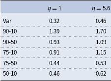
Note: Variances are calculated using log wages within the abstract task. The rest are log differences between corresponding percentiles of wage. So for example 1.39 means that the ratio of 90th percentile to 10th percentile of wages is $e^{1.39}$
. The percentage change of the ratio is approximately the difference of two steady states.
$e^{1.39}$
. The percentage change of the ratio is approximately the difference of two steady states.
5.2. Transition dynamics
This section discusses the entire path of the solution of the model and investigates whether the model could generate an acceleration of the growth of wage dispersion within the abstract task throughout the transition path. We know from the steady state analysis above that an investment-specific technical change embodied by an increase in $q$
could drive a higher level of investment and capital stock, which replace the input of labor in the routine task. So lower types of workers who are replaced by machines then have to work on the abstract task, which mechanically widens wage inequality within the abstract task due to the composition effect. However, the facts in Section 2 demonstrate that wage inequality was not increasing linearly in the past four decades but featured an acceleration in its growth starting from 2000. To understand this using our task-based framework requires a complete characterization of the behavior of the model when it transits from one steady state to another.
$q$
could drive a higher level of investment and capital stock, which replace the input of labor in the routine task. So lower types of workers who are replaced by machines then have to work on the abstract task, which mechanically widens wage inequality within the abstract task due to the composition effect. However, the facts in Section 2 demonstrate that wage inequality was not increasing linearly in the past four decades but featured an acceleration in its growth starting from 2000. To understand this using our task-based framework requires a complete characterization of the behavior of the model when it transits from one steady state to another.
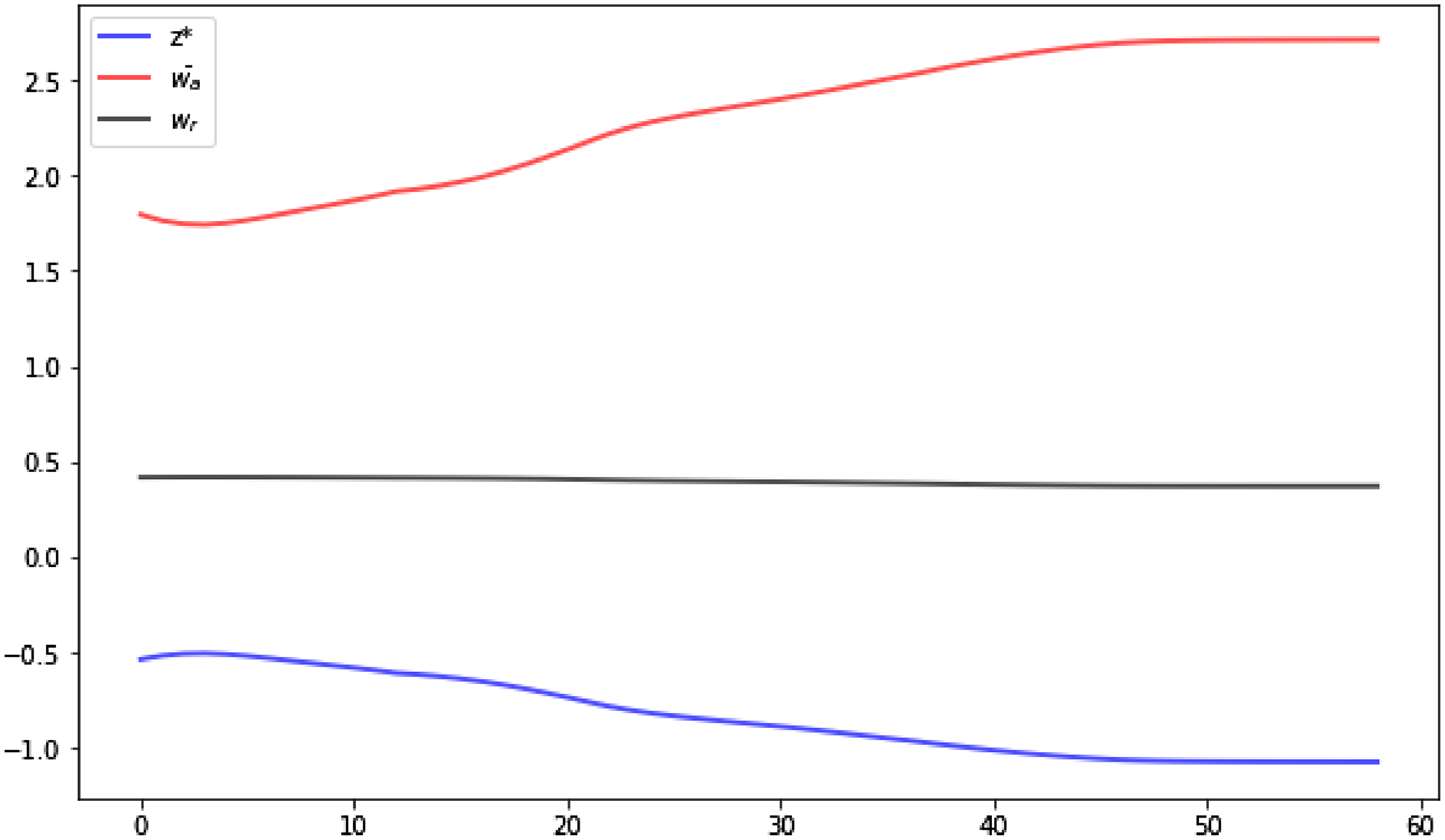
Figure 5. Transition dynamics of model solution.
Note: $z^{*}$
(blue line) is the threshold value of
$z^{*}$
(blue line) is the threshold value of $z$
that determines the assignment of workers;
$z$
that determines the assignment of workers; $wa$
(red line) and
$wa$
(red line) and $wr$
black line) denote the mean wage rate of labor for abstract and routine tasks.
$wr$
black line) denote the mean wage rate of labor for abstract and routine tasks.
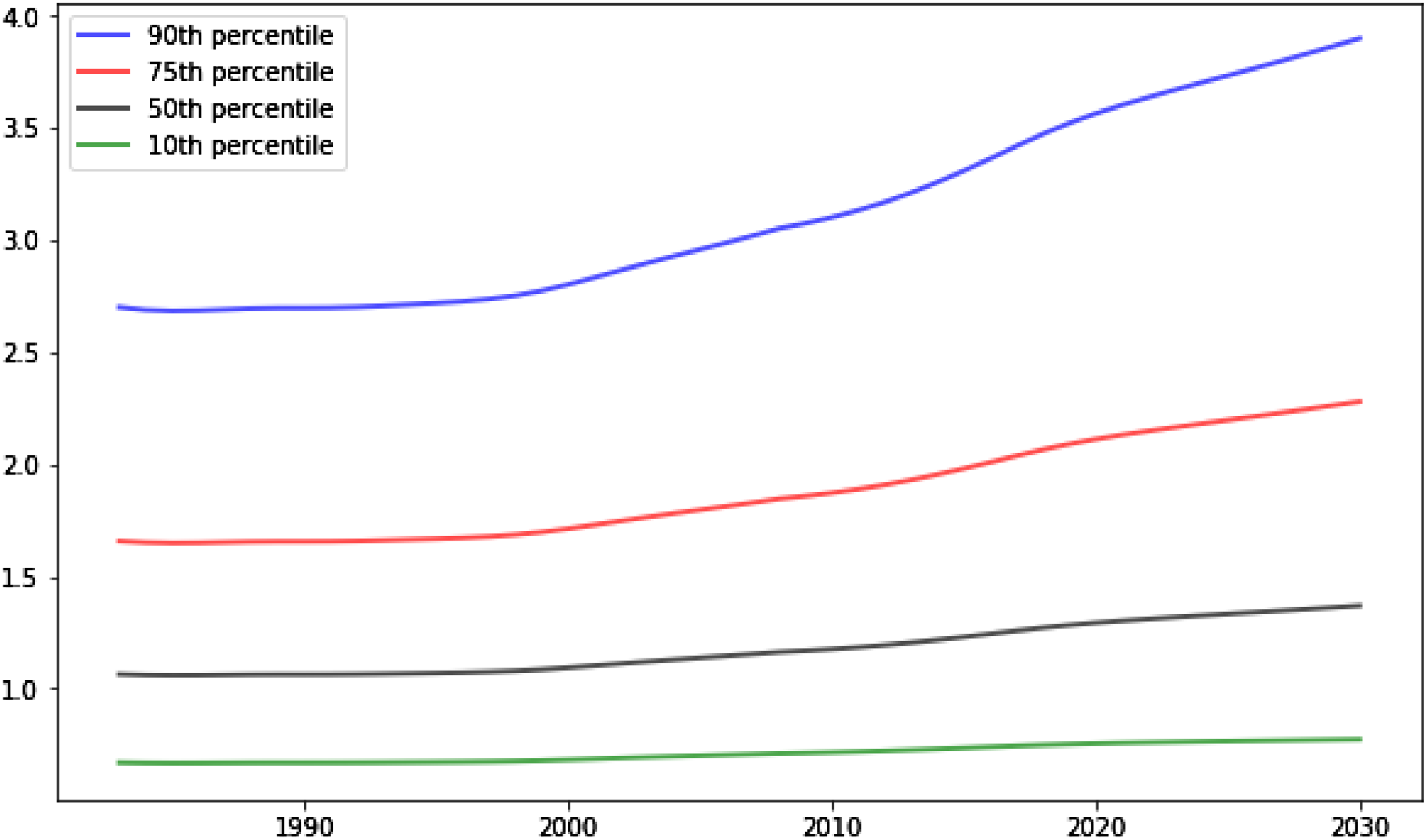
Figure 6. Wage distribution in the abstract task.
Note: The figure displays the transition of the 90/75/50/10th percentile of wage in the abstract task solved from the model.
Fig. 5 displays the transition dynamics of the model solution. The main object of interest is the threshold values of worker type $z^{*}$
, which determine the allocation of workers in the two tasks. Not surprisingly,
$z^{*}$
, which determine the allocation of workers in the two tasks. Not surprisingly, $z^{*}$
transits from a high to a low level almost monotonically. But one appealing finding is that the trajectory of
$z^{*}$
transits from a high to a low level almost monotonically. But one appealing finding is that the trajectory of $z^{*}$
is significantly convex, with largely a flat level in the first 15 periods and an accelerated declining rate after that. The kink arises in the second half of the 1990s, coinciding with the timing of the acceleration of wage inequality. Since in this model wage inequality within the abstract task is entirely driven by the composition effect induced by reallocation of labor from the routine to the abstract task, this result suggests that the model might be able to generate a nonlinear trend of wage inequality during the transition.
$z^{*}$
is significantly convex, with largely a flat level in the first 15 periods and an accelerated declining rate after that. The kink arises in the second half of the 1990s, coinciding with the timing of the acceleration of wage inequality. Since in this model wage inequality within the abstract task is entirely driven by the composition effect induced by reallocation of labor from the routine to the abstract task, this result suggests that the model might be able to generate a nonlinear trend of wage inequality during the transition.
Consistent with the conjecture above, I find that the wage distribution in the abstract task shifts up at an accelerated rate, and this acceleration is more salient for the higher percentiles of wage. Fig. 6 shows the distribution of wages measured by varying percentiles throughout the transition path. The 90th percentile of wage exhibits a remarkable kink at the end of the 1990s, while the 10th percentile of wage is relatively flat. This suggests that wage inequality within the abstract task should rise at an increasing rate. Indeed, various measures of inequality as shown in Fig. 7 reveal that all percentiles of wage in the abstract task shift up relative to the lower percentiles, and the trend of the growth is not linear throughout the transition path but features an acceleration occurring around 2000, which is in line with the empirical facts we find in Section 2.
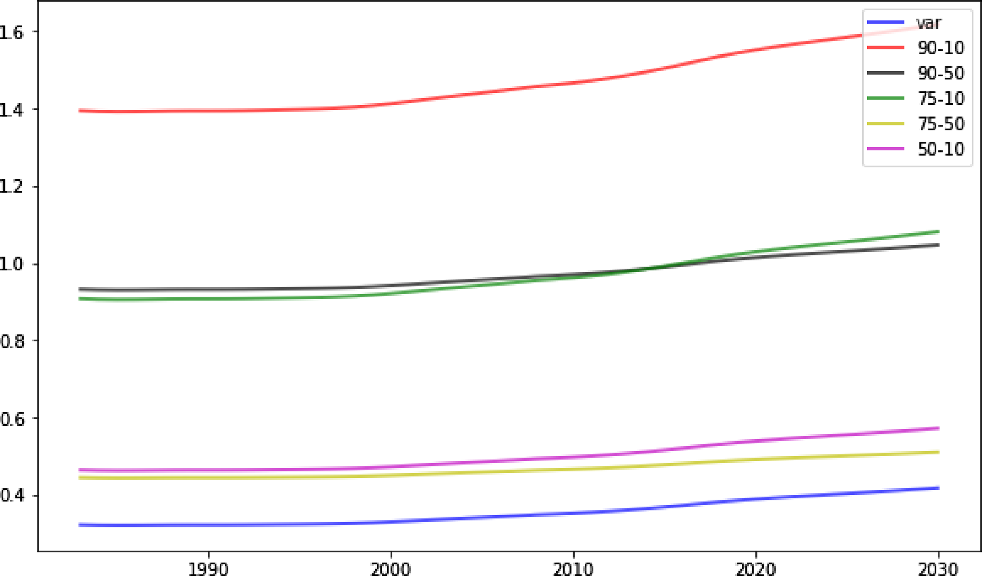
Figure 7. Wage inequality in the abstract task.
Note: The figure displays the transition of different measures of wage inequality in the abstract task. See the note in Table 5 for interpretation of the measures.
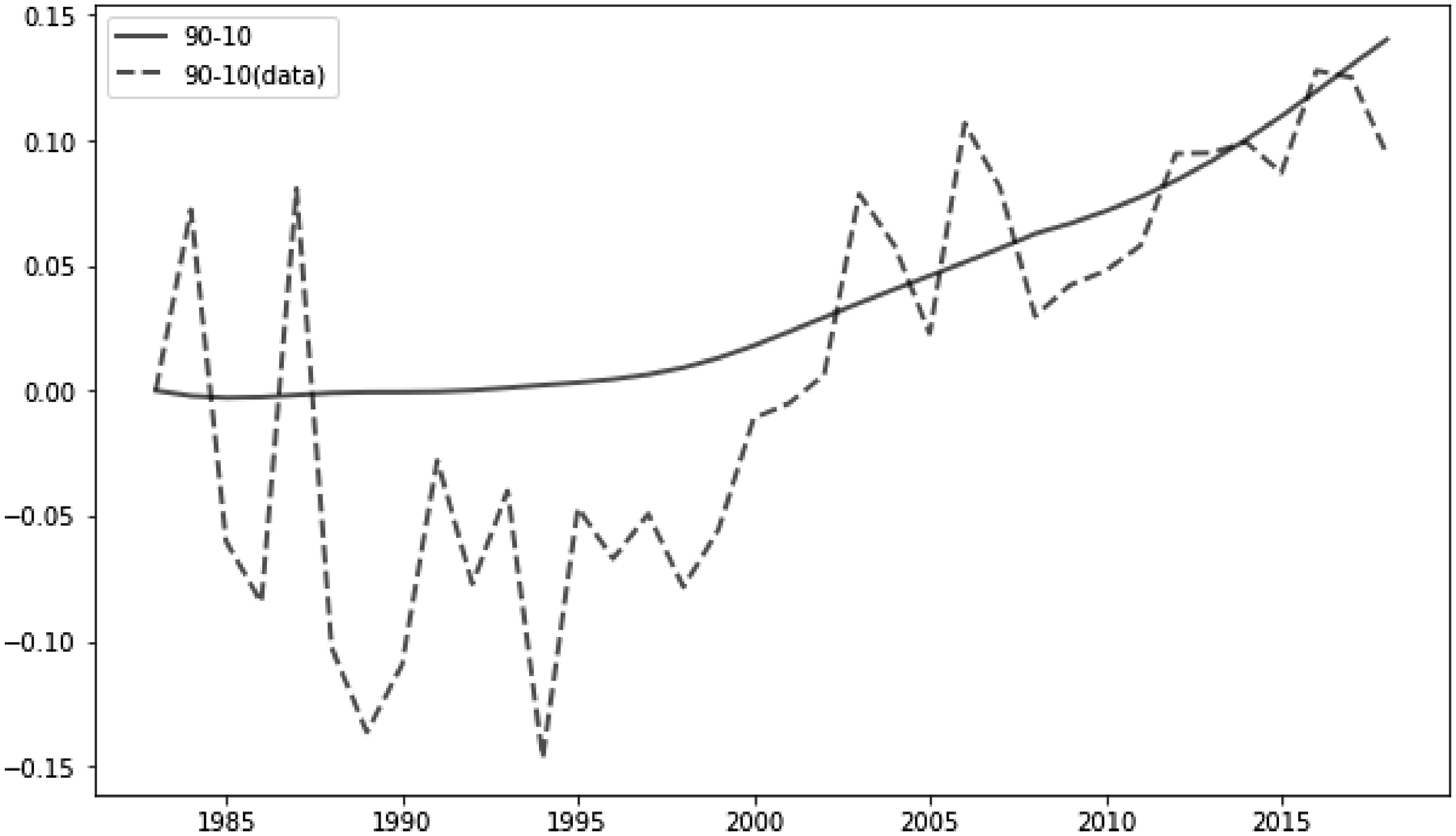
Figure 8. 90-10 wage inequality in the abstract task (model and data).
Note: The solid (dashed) line denotes the log difference between the 90th and 10th percentile of wage in the abstract task throughout the transition path obtained from the model (data). Both measures are normalized to zero in the initial period.
To gain a more straightforward view of how the model maps to the data, Fig. 8 brings the model back to the data and the result suggests the model could match the trend of wage inequality in the abstract task as measured by the log difference between 90th and 10th percentile of wage qualitatively well.Footnote 19 Although the model struggles to capture the bouncing and downward-trending behavior of the data before 2000 but predicts a flat level, it matches well the timing and magnitude of the widening of wage inequality up until now. Given that the wage data in the abstract task is a small sample and the whole sample of skilled workers seems to support a stable and flat trend of wage inequality before 2000, I take the result as a successful test for the model. In the next section, I briefly discuss why this model could work in explaining the nonlinear expansion of wage inequality.
5.3. Discussion
The results of the model imply that a sustained investment-specific technical change could induce a nonlinear expansion path of inequality throughout the transition dynamics. Interestingly, when revisiting the path of $q$
, which is the sole exogenous driving force of the model, we can find that the growth rate of
$q$
, which is the sole exogenous driving force of the model, we can find that the growth rate of $q$
is at a peak around 2000. Thus, the widening of wage inequality actually occurs when the increase in
$q$
is at a peak around 2000. Thus, the widening of wage inequality actually occurs when the increase in $q$
slows down.
$q$
slows down.
This seems counterintuitive because we know that it is the crowding-out effect induced by investment-specific technical change that drives the change of composition of workers, which mechanically enlarges the spread of wage distribution. If this is the case, one might expect the trajectory of wage inequality should largely follow the path of $q$
. In fact, Aghion (Reference Aghion2002) demonstrates that there is essentially a one-to-one mapping between the level of wage inequality and the growth rate of a neutral technical change embodied by an increase in TFP. To understand this, it is useful to examine how the capital stock evolves, because ultimately the higher the capital stock, the more workers with low
$q$
. In fact, Aghion (Reference Aghion2002) demonstrates that there is essentially a one-to-one mapping between the level of wage inequality and the growth rate of a neutral technical change embodied by an increase in TFP. To understand this, it is useful to examine how the capital stock evolves, because ultimately the higher the capital stock, the more workers with low $z$
will be crowded out from the routine task.
$z$
will be crowded out from the routine task.
Fig. 9 shows that the capital stock does not change much before 2000 and rapidly accelerates thereafter. This pattern largely shapes the behavior of other variables, especially the threshold values of $z^{*}$
. Unlike TFP change as in Aghion (Reference Aghion2002), investment-specific technical change features a “lagging” response of investment because when agents perfectly anticipate a sustained growth in
$z^{*}$
. Unlike TFP change as in Aghion (Reference Aghion2002), investment-specific technical change features a “lagging” response of investment because when agents perfectly anticipate a sustained growth in $q$
, which will make the investment cheaper as the process proceeds, they would not immediately invest to redeem the good news, but choose to postpone the investment to the future when the prices are even lower than when the technical change initiates. Consequently, the acceleration in investment occurs after the technical change progresses.
$q$
, which will make the investment cheaper as the process proceeds, they would not immediately invest to redeem the good news, but choose to postpone the investment to the future when the prices are even lower than when the technical change initiates. Consequently, the acceleration in investment occurs after the technical change progresses.
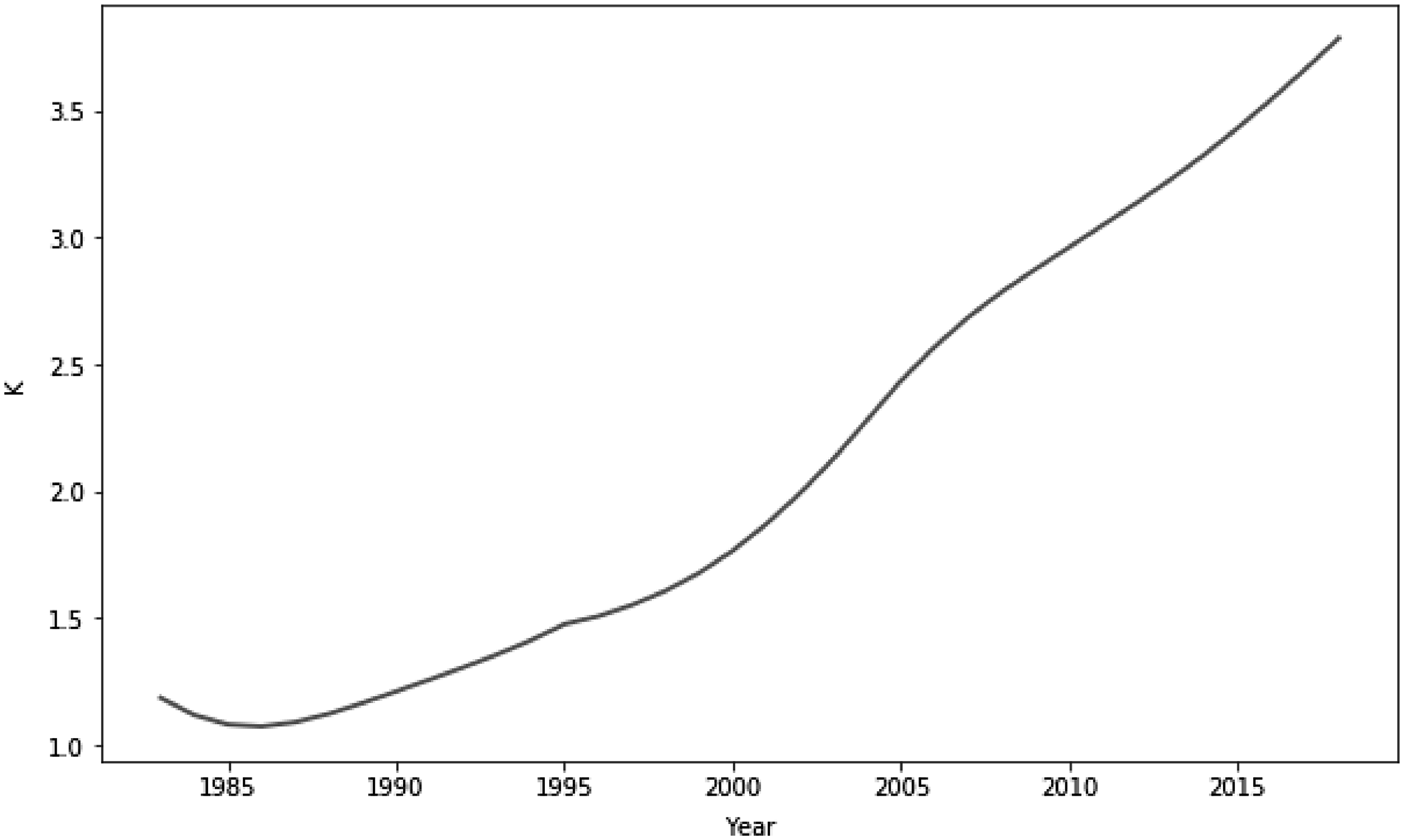
Figure 9. Transition of capital stock.
We know wage inequality in the abstract task is exclusively driven by the composition effect caused by the change of the threshold values of $z^{*}$
.Footnote 20 Then, since the latter is due to the reallocation of labor in the routine task, which is replaced by machines (capital stock), to the abstract task, the fanning-out transition path of capital stock determines that wage inequality in the abstract task also features a nonlinear expansion path throughout the transition.
$z^{*}$
.Footnote 20 Then, since the latter is due to the reallocation of labor in the routine task, which is replaced by machines (capital stock), to the abstract task, the fanning-out transition path of capital stock determines that wage inequality in the abstract task also features a nonlinear expansion path throughout the transition.
In addition, the log-normal distribution of labor efficiencies preserves the convex expansion path of threshold value $z^{*}$
so that the path of wage inequality mimics that of
$z^{*}$
so that the path of wage inequality mimics that of $z^{*}$
. How the results would change when other right-tailed wage distributions and model parameters are used is left to future work, but the quantitative results suggest that the model is able to provide a well-matched timing and magnitude of the change of the trend in wage inequality.
$z^{*}$
. How the results would change when other right-tailed wage distributions and model parameters are used is left to future work, but the quantitative results suggest that the model is able to provide a well-matched timing and magnitude of the change of the trend in wage inequality.
5.4. Broader implications
While I mainly focus on wage inequality (within the abstract task) in this paper, the model is also able to draw implications that are of broader interest in macroeconomic literature and results qualitatively consistent with the data. I discuss in this section the labor share, investment share, and overall inequality and compare them with the data.
Of all the series, labor share is of particular interest because its recent decline triggered numerous works investigating the magnitude and determinants (see e.g., Elsby et al. (Reference Elsby, Hobijn and Şahin2013), Karabarbounis and Neiman (Reference Karabarbounis and Neiman2014)). Since the key mechanism of the model is the replacement of labor by machine, one should expect the model to generate a declining trend of labor share, which is consistent with the observation from data. Indeed, Fig. 10 confirms the good fit by comparing two commonly used series of labor share in the data with the series generated by the baseline model (black dotted line).Footnote 21 Despite the jump of the labor share around 2000 which was probably caused by cyclical factors like IT bubbles, the model successfully captures the declining trend of labor share in the past four decades with quantitatively comparable magnitude relative to the data.
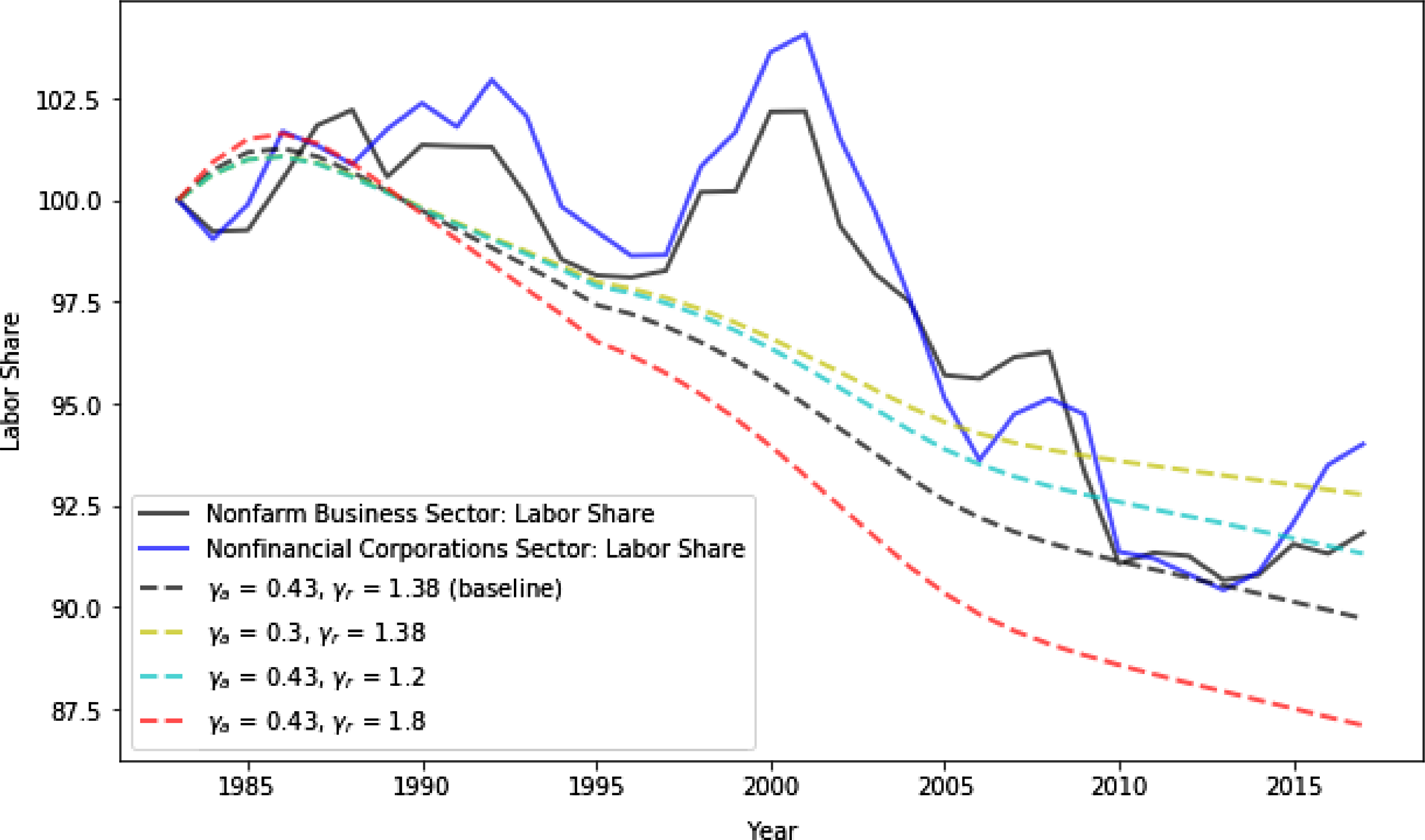
Figure 10. Labor share (1983–2018).
Note: The solid lines denote the labor share of nonfarm business sector and nonfinancial corporation sector reported by BLS. The dotted lines denote the labor share obtained by solving the model under different scenario of elasticities of substitution. All series are normalized to 100 in the initial year (1983).

Figure 11. Investment (equipment) share (1985–2018).
Note: The solid line denotes the investment share of nonresidential equipment reported by BEA. The dotted lines denote the investment share obtained by solving the model under different scenario of elasticities of substitution. All series are normalized to 100 in the initial year (1985).
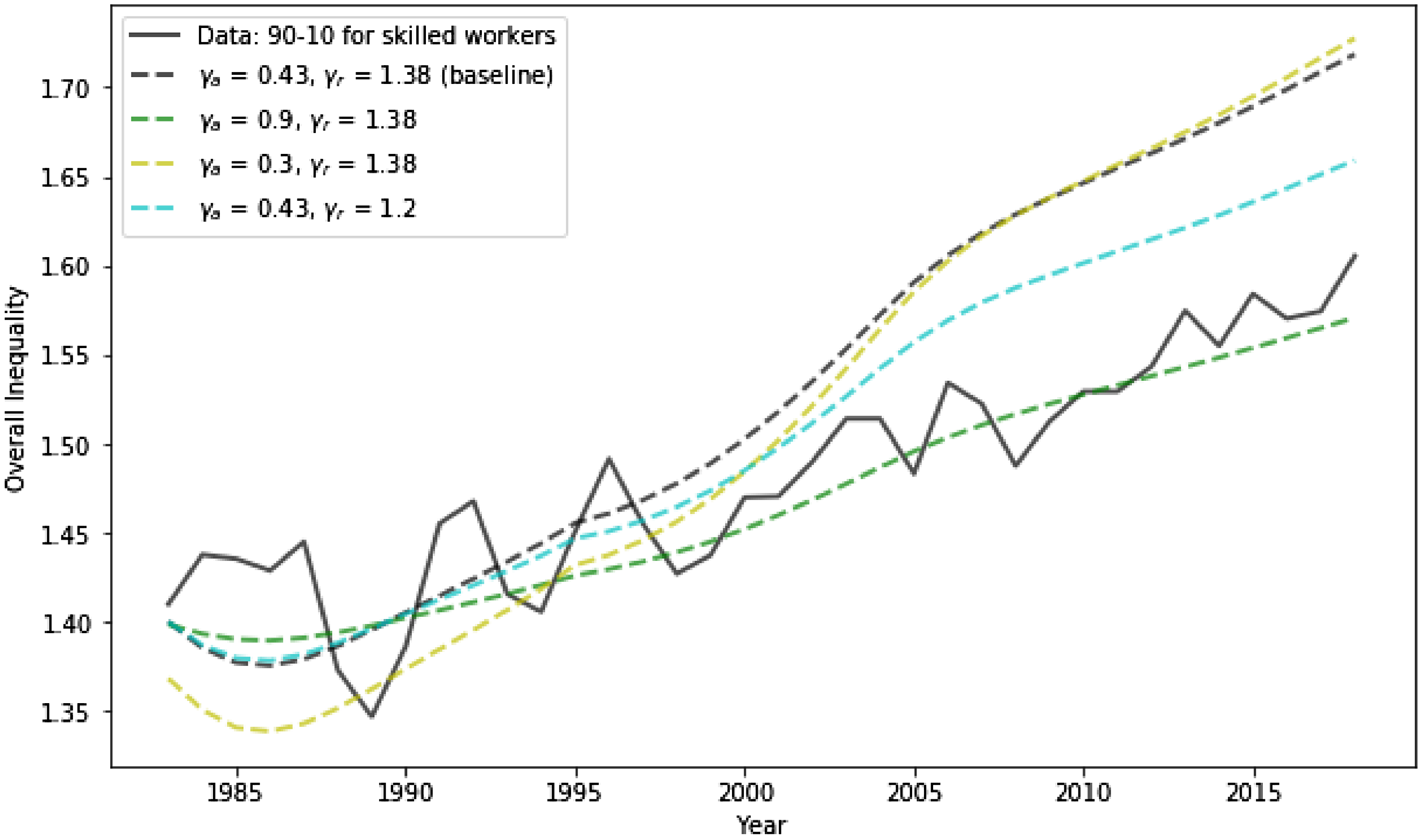
Figure 12. Overall inequality.
Note: The solid line denotes the overall inequality measured by the log difference between 90th percentile and 10th percentile of real wage for skilled workers from CPS ASEC data. The dotted lines denote the the log difference between 90th percentile and 10th percentile of real wage for all workers in the model economy.
In addition, by decreasing or increasing the elasticities of substitution ( $\gamma _{a}$
,
$\gamma _{a}$
, $\gamma _{r}$
), the model is able to give rise to various magnitudes of the decline of labor share, which reflects the flexibility of the theoretical framework to accommodate different measures of labor share in the data. Therefore, the results suggest a successful and straightforward mechanism both qualitatively and quantitatively in explaining the declining trend of labor share in the last four decades, which is the replacement of labor by machines induced by investment-specific technological change. This paper is not the first one to propose this mechanism; rather, it was extensively examined in the literature, and there is a considerable consensus that the acceleration of investment-specific technological change contributes to the recent decline of labor share.Footnote
22
The implication of the model in this paper, nevertheless, serves as a fairly rigorously conducted robustness check of the theory.
$\gamma _{r}$
), the model is able to give rise to various magnitudes of the decline of labor share, which reflects the flexibility of the theoretical framework to accommodate different measures of labor share in the data. Therefore, the results suggest a successful and straightforward mechanism both qualitatively and quantitatively in explaining the declining trend of labor share in the last four decades, which is the replacement of labor by machines induced by investment-specific technological change. This paper is not the first one to propose this mechanism; rather, it was extensively examined in the literature, and there is a considerable consensus that the acceleration of investment-specific technological change contributes to the recent decline of labor share.Footnote
22
The implication of the model in this paper, nevertheless, serves as a fairly rigorously conducted robustness check of the theory.
The other relevant series is the investment share, which reflects the flow of marginal increment of capital accumulation rather than the stock. This series is of interest because the investment (in equipment) is directly related to the price of equipment production and stimulated by its decline. Given that we have the full path of relative price of investment goods ( $q_{t}$
), we should expect to replicate fairly well the relative movement of the investment share if the long-run behavior of investment (in equipment) is mostly dependent on its rental rate
$q_{t}$
), we should expect to replicate fairly well the relative movement of the investment share if the long-run behavior of investment (in equipment) is mostly dependent on its rental rate $r$
. Fig. 11 establishes this conjecture by showing the series of investment derived by the model co-move with the empirical counterpart except for a lag. This error is most likely to come from the series of
$r$
. Fig. 11 establishes this conjecture by showing the series of investment derived by the model co-move with the empirical counterpart except for a lag. This error is most likely to come from the series of $q_{t}$
, which might be measure with lag, but the successful replication of the peak and trough of the investment share demonstrates the strong dependence of the investment behavior on the relative price (efficiency), which is consistent with the mainstream in the literature of (investment-specific) technological change.
$q_{t}$
, which might be measure with lag, but the successful replication of the peak and trough of the investment share demonstrates the strong dependence of the investment behavior on the relative price (efficiency), which is consistent with the mainstream in the literature of (investment-specific) technological change.
Fig. 12 displays the last series derived from the model, which is the level of overall inequality measured by the log difference between 90th percentile and 10th percentile of real wage for all workers in the model economy. I compare that with its empirical counterpart for skilled workers because it is the relevant group for the analysis of wage inequality. It should be noted that the overall inequality increases for completely distinct reason from within-group inequality. The latter is driven by composition effect, while the former is all price effect because the rank of individual total wage is unchanged by any reallocation in this economy. The result should therefore be viewed as a complementary qualitative implication of the model which demonstrates how the other effect should play a role in determining the entirety of wage inequality, but the quantitative significance should not be taken very seriously.
6. Conclusions
The analysis in this paper was motivated by empirical evidence that the growth rate of wage inequality has significantly accelerated since 2000. The main contribution of the paper is to link the task-based framework to wage inequality, which was not fully explored in previous literature. Using a task-based framework as in ALM, I find the change in the trend of wage differential for the whole group of skilled workers was exclusively driven by that within the nonroutine analytic task.
A parsimonious theoretic framework of labor reallocation across tasks based on vom Lehn (Reference vom Lehn2020) was then developed. In this model, the labor reallocation is induced by an ongoing investment-specific technical change which features a drop in the prices of investment goods. Workers in the routine task are replaced by cheaper machines and then have to relocate to the abstract task. Since workers are heterogeneous in the endowment of efficiency units of labor in the abstract task and the assignment of workers to tasks is based on the comparative advantage, the marginal entrants to the abstract task are lower types of $z$
compared to the incumbents. Wage inequality in the abstract task is then widened due to the composition effect. In addition, since economic agents tend to postpone the investment in machines after the ongoing investment-specific technical change takes place for a while, the expansion path of wage inequality is not linear but features an acceleration of wage dispersion in the middle of the technical change. Despite its simple setup, the quantitative results suggest that the model is able to provide a well-matched timing and magnitude of the change in the trend of wage inequality that is observed in the data.
$z$
compared to the incumbents. Wage inequality in the abstract task is then widened due to the composition effect. In addition, since economic agents tend to postpone the investment in machines after the ongoing investment-specific technical change takes place for a while, the expansion path of wage inequality is not linear but features an acceleration of wage dispersion in the middle of the technical change. Despite its simple setup, the quantitative results suggest that the model is able to provide a well-matched timing and magnitude of the change in the trend of wage inequality that is observed in the data.
Acknowledgements
I thank Bart Hobijn for his invaluable motivation and advices on this project. I also thank useful commentsfrom the editor, Gustavo Ventura, Natalia Kovrijnykh, and Siyu Shi. All errors are on my own.
Competing interests
The author is employed at School of Economics, University of Edinburgh.
APPENDIX A. SOLUTION METHOD
A.1. Solving the steady states
Suppose the threshold value of $z$
is
$z$
is $z^{*}$
in the steady state, it must satisfy the following indifference condition:
$z^{*}$
in the steady state, it must satisfy the following indifference condition:
 \begin{equation} w_{a} e^{\alpha _{a}z^{*}}= w_{r} \end{equation}
This reduces to
 \begin{equation} z^{*} = \frac{lnw_{r} - lnw_{a}}{\alpha _{a}} \end{equation}
Then, solving the Euler equation (9) evaluated at steady state gives rise to steady state value of $r$
. Since
$r$
. Since $N_{a}$
and
$N_{a}$
and $N_{r}$
can be expressed as a function of
$N_{r}$
can be expressed as a function of $z$
by utilizing expectation of truncated log-normal distribution and CDF of standard normal distribution, equation (A2), combined with equations (10)–(12), consists of a system of four equations and four unknowns, namely
$z$
by utilizing expectation of truncated log-normal distribution and CDF of standard normal distribution, equation (A2), combined with equations (10)–(12), consists of a system of four equations and four unknowns, namely $z^{*}$
,
$z^{*}$
, $w_{a}$
,
$w_{a}$
, $w_{r}$
,
$w_{r}$
, $K$
.
$K$
.
A.2. Solving the transition
The solution to the full model can be found using the standard shooting algorithm. To be specific, I proceed by the following steps:
-
1. Let the first period be in the initial steady state, so we know all the variables in the first period. Then consider the Euler equation (9) and substitute
$C$
by
$K$
and
$Y$
using the resource constraint (8). -
2. Guess a
$K_{2}$
and solve the system of equations (10)–(12) for period 2, so we know
$r_{2}$
. Then (9) gives
$K_{3}$
and following the same procedure I obtain the entire path of the model solution up to any period given the guess of
$K_{2}$
. -
3. Allow roughly two decades of burn-in time. I adjust
$K_{2}$
such that the model hits the terminal steady state at period 67. If the model does not converge up to an infinitesimal tolerance value, adjust the burn-in time by 1 period.


APPENDIX B. DEFINITION OF DOT TASKS AND CLASSIFICATION OF COC OCCUPATIONS
In this appendix, I describe how the classification of tasks is constructed and mapped to occupations using the consistent three-digit COC in CPS data. The following table displays the definitions of the five categories of tasks and variables used to measure the intensity of tasks put forth in Section 2. Using the values of measures of task intensity by the 1977 DOT, I rank the occupations based on consistent three-digit COC in CPS data extracted from IPUMS for each category of task. For example, the economist might rank the first in the nonroutine analytic task because it has the highest score on MATH but rank the last in the routine manual task because it has the lowest score on FINGDEX. I then categorize each occupation to the task that ranks the highest for this occupation. Economist, for example, is attributed to the nonroutine analytic task, since its MATH score ranks higher than any of the other scores. Examples of occupations/tasks from CPS data (consistent three-digit COC on the 1990 basis (occ1990)) are presented in the last column of the table.
Table B.1. Definitions and examples of tasks from ALM (2003)
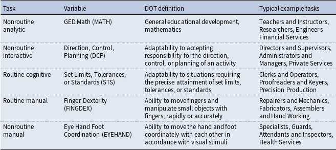
Source: ALM (2003) and IPUMS.
Note: The variables used to measure the intensity of tasks follow ALM (2003) based on definition of tasks from 1977 Dictionary of Occupational Titles. The examples of occupations/tasks are from IPUMS consistent three-digit Census Occupation Code (COC) on the 1990 basis (occ1990).
APPENDIX C. TECHNICAL DETAILS
In this appendix, I provide a rigorous analytic derivation of why measures of wage inequality in the abstract task depend on $z^{*}$
but not wage rates. I use
$z^{*}$
but not wage rates. I use $90 - 10$
wage differential defined in Table 5 as an example, but the derivation follows for all measures of wage differential between percentiles.
$90 - 10$
wage differential defined in Table 5 as an example, but the derivation follows for all measures of wage differential between percentiles.
The logarithm of ratio of the wage for the 90th percentile and 10th percentile of worker in the abstract task the following:
 \begin{equation} log \left(\frac{w_{at} e^{\alpha _{a} z^{90}_{t}}}{{w_{at} e^{\alpha _{a} z^{10}_{t}}}}\right) = \alpha _{a} \!\left(z^{90}_{t}-z^{10}_{t}\right) \end{equation}
where $z^{90}_{t}$
(
$z^{90}_{t}$
( $z^{10}_{t}$
) is the 90th (10th) percentile of
$z^{10}_{t}$
) is the 90th (10th) percentile of $z$
in the abstract task, which satisfy
$z$
in the abstract task, which satisfy
 \begin{equation} \frac{1}{1-\Phi (z^{*}_{t})} \int _{z^{*}_{t}}^{z^{90}_{t}} d \Phi (z) = 90 \end{equation}
 \begin{equation} \frac{1}{1-\Phi (z^{*}_{t})} \int _{z^{*}_{t}}^{z^{10}_{t}} d \Phi (z) = 10 \end{equation}
where $z^{*}_{t}$
is the threshold value at time
$z^{*}_{t}$
is the threshold value at time $t$
. Totally differentiating equation (C2) with respect to
$t$
. Totally differentiating equation (C2) with respect to $t$
gives
$t$
gives
 \begin{equation} \frac{\Phi (z^{*}_{t})}{(1-\Phi (z^{*}_{t}))^{2}} \frac{d z^{*}_{t}}{dt} \int _{z^{*}_{t}}^{z^{90}_{t}} d \Phi (z) + \frac{1}{1-\Phi (z^{*}_{t})} \left[\phi (z^{90}_{t})\frac{d z^{90}_{t}}{dt} - \phi (z^{*}_{t})\frac{d z^{*}_{t}}{dt}\right] = 0 \end{equation}
Rearrange and we get
 \begin{equation} \frac{d z^{90}_{t}}{dt} = -89 \frac{\phi (z^{*}_{t})}{\phi (z^{90}_{t})} \frac{d z^{*}_{t}}{dt} \end{equation}
Similar procedure for the 10th percentile gives
 \begin{equation} \frac{d z^{10}_{t}}{dt} = -9 \frac{\phi (z^{*}_{t})}{\phi (z^{10}_{t})} \frac{d z^{*}_{t}}{dt} \end{equation}
Therefore, using equation (C1) and applying (C4) and (C5), the time derivative of the logarithm of ratio is
 \begin{equation} \frac{d}{dt}\!\left(\alpha _{a} \left(z^{90}_{t}-z^{10}_{t}\right)\right) = \alpha _{a} \frac{d z^{*}_{t}}{dt} \phi (z^{*}_{t}) \left(\frac{9}{\phi (z^{10}_{t})} - \frac{89}{\phi (z^{90}_{t})}\right) \end{equation}


