


1. Introduction
Helical vortices occur in devices containing rotating wings, which include wind turbines, helicopters, ship propellers and other important engineering applications. In a large-scale wind farm, the wake flow of a wind turbine affects the incoming flow of the wind turbines behind it. As a result, the performance of a wind turbine in the wake of other wind turbines is often much smaller than that of a frontal wind turbine (Lee & Fields Reference Lee and Fields2021).
The wake flow of a wind turbine is dominated by the helical vortices generated from the tip of the rotor blades. The helical vortices are subject to several instabilities, which can be classified into two types depending on the wavelength of the disturbance: (i) the long-wave instability, in which the wavelength of the disturbance is much larger than the vortex-core size; and (ii) the short-wave instability, in which the wavelength of the disturbance is comparable to the vortex-core size. The long-wave instability includes the pairing instability (Quaranta, Bolnot & Leweke Reference Quaranta, Bolnot and Leweke2015; Quaranta et al. Reference Quaranta, Brynjell-Rahkola, Leweke and Henningson2019), the Crow instability (Crow Reference Crow1970) and the mutual inductance mode (Widnall Reference Widnall1972). Their mechanisms can be understood in the framework of the vortex-filament approximation (Crow Reference Crow1970; Widnall Reference Widnall1972; Gupta & Loewy Reference Gupta and Loewy1974); the vorticity distribution in the vortex core does not affect the stability properties essentially, although the effective size of the vortex core affects slightly the growth rate through a cutoff in the Biot–Savart integral. In contrast, the properties of the short-wave instability, which includes the elliptic instability (Kerswell Reference Kerswell2002; Blanco-Rodríguez & Le Dizès Reference Blanco-Rodríguez and Le Dizès2016) and the curvature instability (Hattori & Fukumoto Reference Hattori and Fukumoto2003; Fukumoto & Hattori Reference Fukumoto and Hattori2005; Hattori & Fukumoto Reference Hattori and Fukumoto2009, Reference Hattori and Fukumoto2010, Reference Hattori and Fukumoto2011, Reference Hattori and Fukumoto2012, Reference Hattori and Fukumoto2014; Blanco-Rodríguez & Le Dizès Reference Blanco-Rodríguez and Le Dizès2017; Hattori, Blanco-Rodríguez & Le Dizès Reference Hattori, Blanco-Rodríguez and Le Dizès2019), are dictated by the vorticity distribution inside the vortex core. Recent works tried to promote breakdown and turbulent transition for wake recovery by exciting long-wave instability of helical vortices (Abraham, Castillo-Castellanos & Leweke Reference Abraham, Castillo-Castellanos and Leweke2023; Ramos-García et al. Reference Ramos-García, Abraham, Leweke and Sørensen2023). In this regard, understanding the nonlinear dynamics of helical vortices after the linear regime of the long-wave instability is important not only in prediction of wake recovery but also in optimizing the method of exciting the instability to maximize the effects.
There have been many works on the dynamics of helical vortices. The long-wave instability of a single helical vortex has been captured experimentally by Quaranta et al. (Reference Quaranta, Bolnot and Leweke2015); they also showed that the unstable modes are explained by the pairing instability. Alekseenko et al. (Reference Alekseenko, Kuibin, Shtork, Skripkin and Tsoy2016) studied the motion of a helical vortex created in a swirling flow; they showed that vortex reconnection results in either an isolated vortex ring or a vortex ring linked with the main helical vortex. However, the detailed process after the reconnection, which can lead to turbulent transition, remains unexplored. Direct numerical simulation is an ideal method to explore this process because it has several advantages over experiments; the parameters and the velocity distribution specifying the base flow and the disturbances can be prescribed at our will, while precise data of flow fields are available.
In this paper, we study the nonlinear evolution of a single helical vortex disturbed by a long-wave-instability mode by direct numerical simulation. Our objectives are to clarify the detailed processes of vortex reconnection observed by Alekseenko et al. (Reference Alekseenko, Kuibin, Shtork, Skripkin and Tsoy2016) and to explore the dynamics after them leading to possible turbulent transition and breakdown of the helical vortex, which are often difficult to analyse in the experiments. We will show that the evolution after the reconnection depends crucially on the pitch of the helical vortex.
2. Numerical procedure
2.1. Statement of the problem
We consider the time evolution of a helical vortex disturbed by a long-wave-instability mode in an incompressible viscous fluid. The base flow is a helical vortex with constant pitch in a cylindrical coordinate system  $(r, \theta, z)$ (figure 1). The helical vortex extends infinitely in both the positive and negative $z$ directions. The radius of the cylinder of which surface includes the centreline helix is $R$, while the spatial period in the $z$ direction is $2{\rm \pi} L$; we call $L/R$ the reduced pitch as in Delbende, Rossi & Daube (Reference Delbende, Rossi and Daube2012). The vorticity is concentrated in the vicinity of the centreline helix.
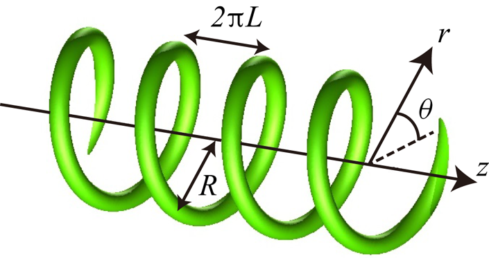
Figure 1. Schematic diagram of helical vortex in the cylindrical coordinate system. The helical vortex extends infinitely in the  $+z$ and $-z$ directions with constant reduced pitch $L/R$.
2.2. Numerical methods
The numerical procedure consists of three steps: (i) a base flow is obtained as a quasisteady state by solving the Navier–Stokes equations; (ii) a long-wave-instability mode is obtained by integrating the linearized Navier–Stokes equations for a sufficiently long time; and (iii) the time evolution of a helical vortex disturbed by the long-wave-instability mode is obtained by solving the Navier–Stokes equations. The numerical method for solving the Navier–Stokes equations is similar to that used in Hattori et al. (Reference Hattori, Blanco-Rodríguez and Le Dizès2019). Namely, for the spatial discretization, the sixth-order accurate compact scheme (Lele Reference Lele1992) was used in the  $r$ direction, while the Fourier spectral method was used in the $\theta$ and $z$ directions. The Poisson equation was decomposed into a set of ordinary differential equations for a single Fourier mode, which were also solved by the sixth-order accurate compact scheme. For the temporal discretization, the Crank–Nicolson scheme was used for the viscous terms, while the second-order Adams–Bashforth method was used for the other terms.
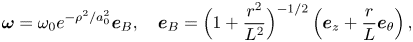
In the first step, the initial vorticity field is given by a Gaussian distribution:
 \begin{equation} \boldsymbol{\omega} =
\omega_0 e^{-\rho^2/a_0^2} \boldsymbol{e}_B, \quad
\boldsymbol{e}_B =
\Big(1+\frac{r^2}{L^2}\Big)^{{-}1/2}\left(\boldsymbol{e}_z+\frac{r}{L}\boldsymbol{e}_\theta\right),
\end{equation}
\begin{equation} \boldsymbol{\omega} =
\omega_0 e^{-\rho^2/a_0^2} \boldsymbol{e}_B, \quad
\boldsymbol{e}_B =
\Big(1+\frac{r^2}{L^2}\Big)^{{-}1/2}\left(\boldsymbol{e}_z+\frac{r}{L}\boldsymbol{e}_\theta\right),
\end{equation}
where  $\rho$ is the distance from the centreline helix, $\omega_0$ is the maximum vorticity, $a_0$ is the core radius, and $\boldsymbol{e}_z$ and $\boldsymbol{e}_\theta$ are the unit vectors in the $z$ and $\theta$ directions, respectively. It is pointed out that $\boldsymbol {e}_B$ is tangential to the centreline helix when $r=R$. The above initial condition is not a steady solution even in a suitable rotating and/or translating frame taking account of the motion of the helical vortex due to the self-induced velocity. However, it reaches a quasisteady state after a certain long time through a relaxation process due to viscous diffusion (Selçuk, Delbende & Rossi Reference Selçuk, Delbende and Rossi2017). The initial radius of the vortex core grows with time approximately as $a^2 = a_0^2 + 4\nu t$, where $\nu$ is the kinematic viscosity and t is the time; thus, $a_0$ was chosen so that the value of $a$ after relaxation becomes a prescribed value.
In the second step, we move to an inertial frame translating with the helical vortex in which it is quasisteady. The so-called ‘frozen-in’ assumption is employed: the time evolution of the base flow obtained in the first step is neglected because its time scale is much larger than the instability. Thanks to the helical symmetry of the base flow, the linear disturbances can be decomposed into modes of the following form which evolve independently:
 \begin{equation} \boldsymbol{u}'(r, \theta, z, t) = \hat{\boldsymbol{u}}(r, \varphi, t) {\rm e}^{{\rm i} k_z z} + \mbox{c.c.}, \end{equation}
where  $\varphi =\theta -(z/L)$ and $k_z$ is the wavenumber in the $z$ direction. For the initial disturbances, we chose a single mode with a velocity distribution $\hat {\boldsymbol {u}}$ randomized and concentrated near the vortex core. Then, by integrating the Navier–Stokes equations linearized about the frozen-in base flow for a sufficiently long time, the most unstable eigenmode is obtained as it becomes much larger than the other modes.
In the third step, the initial condition was obtained by adding the unstable mode obtained in the second step with a small amplitude to the base flow. It is pointed out that in the first and third steps the equations are solved in the static frame of reference in which the flow is at rest at infinity, while the equations in the moving frame as explained above are solved in the second step.
The simulation parameters were chosen as follows. The Reynolds number based on the circulation  $\varGamma$ of the helical vortex was $Re_\varGamma =\varGamma /\nu =15\,700$ in the first and second steps; it is reduced to $Re_\varGamma =3925$ in the third step because small-scale structures which emerge after turbulent transition could not be resolved sufficiently at $Re_\varGamma =15\,700$. The core size of the helical vortex normalized by the curvature radius $(R^2+L^2)/R$ was set to $aR/(R^2+L^2)=0.1$. Two values of the reduced pitch were considered: $L/R=0.2$ and $0.3$. The wavenumber of the disturbance is set to $k_zL=1/2$, at which the growth rate of the long-wave instability is maximum (Widnall Reference Widnall1972; Quaranta et al. Reference Quaranta, Bolnot and Leweke2015). For the domain of calculation, the outer boundary was placed far away from the helical vortex at $r=100R$ to minimize the effect of the slip boundary conditions using stretching grids in the $r$ direction; the axial size of the domain was $4{\rm \pi} L$ to accommodate the wavenumber $k_zL=1/2$. The minimum grid size in $r$ was $\Delta r_{{min}}=4.75 \times 10^{-3}R$, while the grid size in $z$ was $4.91 \times 10^{-3}R$. The number of grid points was $N_r \times N_\theta \times N_z= 695 \times 960 \times 256$ for $L/R=0.2$, while $N_z$ was replaced with $384$ for $L/R=0.3$. The values in the rest of the paper are scaled by the circulation $\varGamma$ and the radius of the cylinder $R$ unless stated explicitly. Throughout the simulation the impulse, which is an invariant in viscous flows, was conserved within $6.4\times 10^{-5}\,\%$ and $2.3 \times 10^{-2}\,\%$ errors for $L/R=0.2$ and $0.3$, respectively, confirming the sufficient accuracy of the numerical simulation.
2.3. Linear instability
Here we briefly summarize the results on the long-wave instability. The growth rates turned out to be  $\sigma =0.236$ and $0.504$ for $L/R=0.3$ and $0.2$, respectively. When normalized by $h=2{\rm \pi} L$ instead of $R$ as the length scale as in Quaranta et al. (Reference Quaranta, Bolnot and Leweke2015), they are $2h^2 \sigma /\varGamma = 1.68$ and $1.59$ for $L/R=0.3$ and $0.2$, respectively; they are close to the theoretical value ${\rm \pi} /2$ and the improved theoretical values given by (2.13) of Quaranta et al. (Reference Quaranta, Bolnot and Leweke2015):
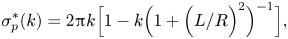 \begin{equation} \sigma_p^\ast(k)=2{\rm \pi}
k \Big[1-k\Big(1+\Big(L/R\Big)^2\Big)^{{-}1}\Big],
\end{equation}
\begin{equation} \sigma_p^\ast(k)=2{\rm \pi}
k \Big[1-k\Big(1+\Big(L/R\Big)^2\Big)^{{-}1}\Big],
\end{equation}
which gives  $1.70$ and $1.63$, respectively, at $k=1/2$. In figure 2, the mode structures for $L/R=0.3$ and $0.2$ are shown by contours of $\boldsymbol {\omega }'\boldsymbol {\cdot } \boldsymbol {e}_B$, where ${\boldsymbol{\omega}}'$ is the vorticity of the disturbance, on a plane perpendicular to $\boldsymbol {e}_B$ at $r=R$, while the origin coincides with the centreline helix. In this figure, the unit vectors are chosen as $\boldsymbol {e}_x = \boldsymbol {e}_r$ and $\boldsymbol {e}_y=\boldsymbol {e}_B\times \boldsymbol {e}_r$. The modes are displacement modes which deform the helix in the direction of the line $y=x$ (Quaranta et al. Reference Quaranta, Bolnot and Leweke2015; Selçuk, Delbende & Rossi Reference Selçuk, Delbende and Rossi2018).
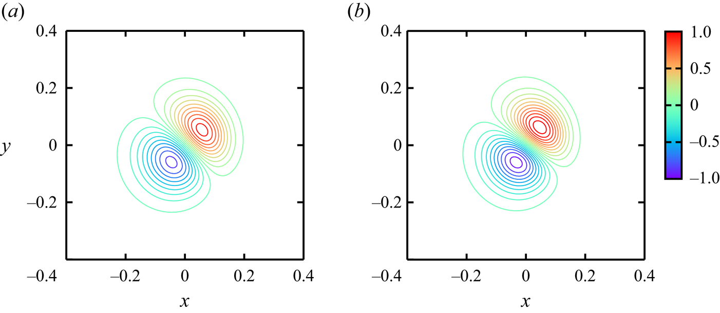
Figure 2. Structure of long-wave-instability mode shown by contours of  $\boldsymbol {\omega }'\boldsymbol {\cdot } \boldsymbol {e}_B$. $k_zL=1/2$. Here (a) $L/R=0.3$, (b) $L/R=0.2$.
3. Results
3.1.  $\textit{Results for }L/R=0.3$

First, we show the results for the larger reduced pitch  $L/R=0.3$. Figure 3 shows the time evolution of the helical vortex visualized by the isosurface of the magnitude of vorticity; it is coloured by the axial component of vorticity $\omega _z$ with red and blue corresponding to positive and negative values, respectively. The value for the isosurface is $|\boldsymbol {\omega }|=0.3\sqrt {\varOmega /R^3}$, where $\varOmega =\int |\boldsymbol {\omega }|^2 \,{\rm d}V$ is the enstrophy and ${\rm d}V=r\,{\rm d}r\,{\rm d}\theta\, {\rm d}z$. In this figure, we set the axial size of the domain for visualization to $8{\rm \pi} L$ to include two adjacent numerical domains; this is to show clearly the structures near the periodic boundaries $z=0$ or $4{\rm \pi} L$. Thus, four pitches of the helical vortex exist initially in the domain for visualization since the periodic unit of the numerical domain involves two pitches.
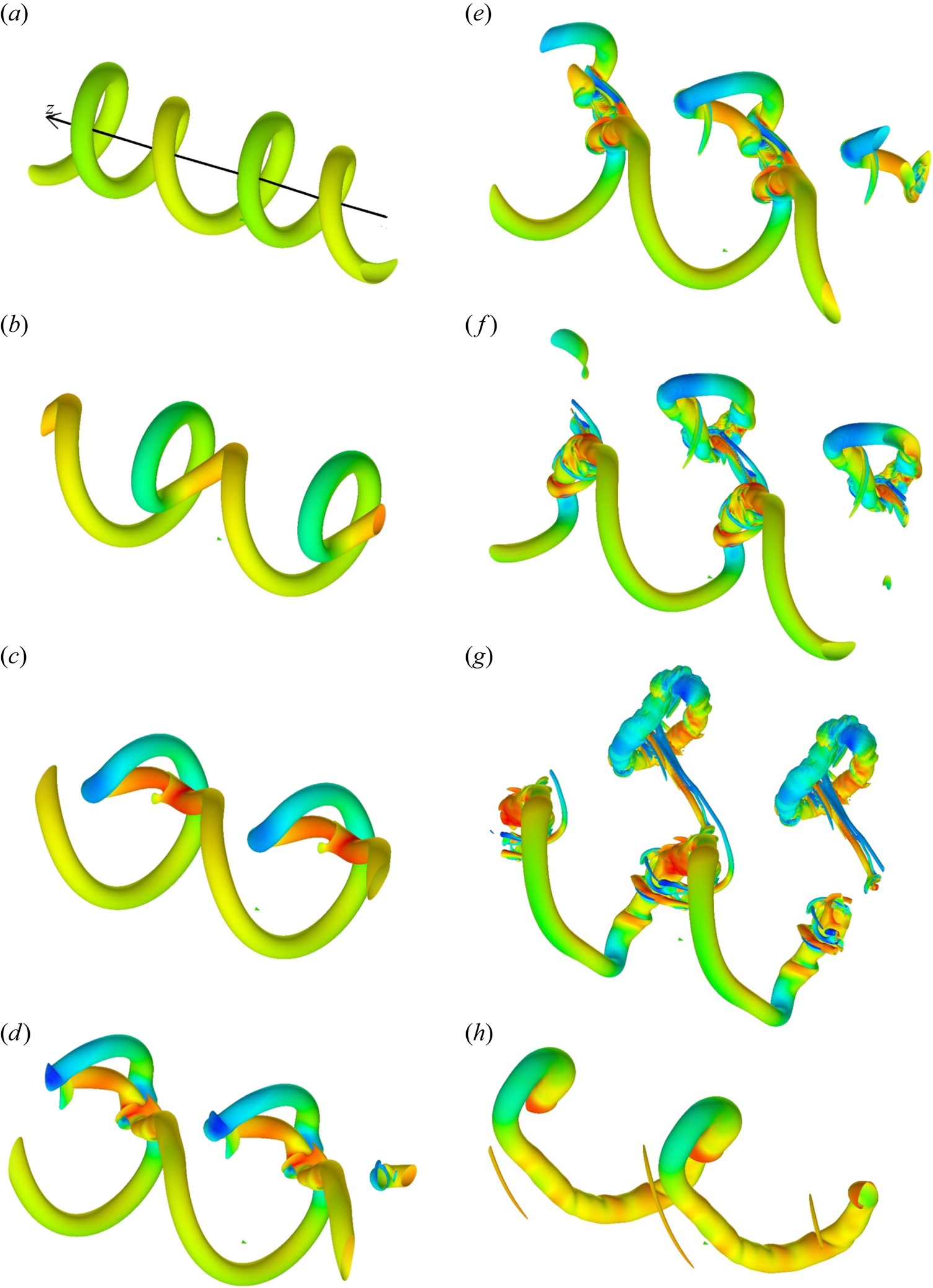
Figure 3. Time evolution of helical vortex with  $L/R=0.3$. The isosurface of the magnitude of vorticity coloured by the axial component of vorticity $\omega _z$. Here $t=$ (a) $17.5$, (b) $23$, (c) $28$, (d) $31$, (e) $33$, (f) $35$, (g) $40$, (h) $65$.
$65$.
At  $t=17.5$ (figure 3a), the instability is still in a linear regime as the distance between the adjacent spirals as well as the distance from the $z$ axis become non-uniform as in Quaranta et al. (Reference Quaranta, Bolnot and Leweke2015). Nonlinear deformation is observed at $t=23$ (figure 3b) as the spirals of smaller radius get close to those of larger radius from inside of the helical vortex, forming vortex-ring-like structures. They move outward owing to the self-induced velocity (figure 3c). Vortex reconnection is in progress from $t \approx 30$ to $t \approx 35$, the so-called ‘bridges’ being observed at $t=31$, $33$ and $35$ (figure 3d–f). Vortex rings detach from the helical vortex and propagate away from it (figure 3g). The pitch of the remaining helical vortex is doubled as the number of spirals is reduced from four at $t=17.5$ (figure 3a) to two at $t=65$ (figure 3h). The time evolution is also shown by the supplementary movie available at https://doi.org/10.1017/jfm.2024.529.
Figures 4(a) and 4(c) show the time evolution of the energy  $E= \int |\boldsymbol {u}|^2 \,{\rm d}V$, the enstrophy $\varOmega$ and the helicity $H=\int \boldsymbol {u}\boldsymbol {\cdot }\boldsymbol {\omega } \,{\rm d}V$. It is pointed out that the non-zero value of the initial helicity is due to the self-induced velocity of the helical vortex, which has an $\boldsymbol {e}_B$ component. The three quantities decrease initially due to viscous diffusion. At $t\approx 22$, however, the enstrophy turns from decreasing to increasing as the adjacent spirals get close and are stretched. The increase accelerates during the vortex reconnection in which thin vortex tubes are generated. The helicity also increases as a result of vortex reconnection. The rate of decay of the energy, which is proportional to the enstrophy as ${\rm d}E/{\rm d}t = -2\nu \varOmega$, increases only slightly during the vortex reconnection as the local maximum of the enstrophy at $t\approx 35$ is smaller than the initial value; transition to turbulence does not occur.
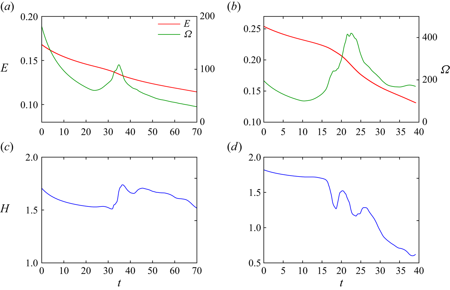
Figure 4. Time evolution of (a,b) energy, enstrophy and (c,d) helicity. Here (a,c)  $L/R=0.3$, (b,d) $L/R=0.2$.
3.2. $\textit{Results for }L/R=0.2$

Next, we show the results for the smaller reduced pitch  $L/R=0.2$. Figure 5 shows the time evolution of the helical vortex visualized in the same way as for $L/R=0.3$, while the direction of the helical vortex is chosen to show the whole process clearly. The linear deformation at $t=8$ (figure 5a) is similar to the case $L/R=0.3$ at $t=17.5$ (figure 3a). At $t=12.5$ (figure 5b), the smaller spirals go through the larger spirals, which resembles the leap-frogging of coaxial vortex rings (Oshima Reference Oshima1978). At $t=14.75$ (figure 5c), there arise two possibilities of vortex reconnection marked by the circles. It turns out that the first reconnection occurs in the upper-left region shown by the red circle as bridges form at
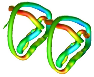
  $t=15.5$ (figure 5d). Vortex rings appear as a result of reconnection; they wrap around the deformed remaining vortex, forming a linked system of vortices (figure 5e), which will be shown in detail later in figure 7. This linkage imposes a topological constraint on the vortex motion forcing strong interaction between vortex tubes. As a result, many thin vortex tubes emerge around the vortex rings and the deformed vortex (figure 5f); finally the flow becomes turbulent as it is dominated by small-scale structures (figure 5g,h). The time evolution is also shown by the supplementary movie.
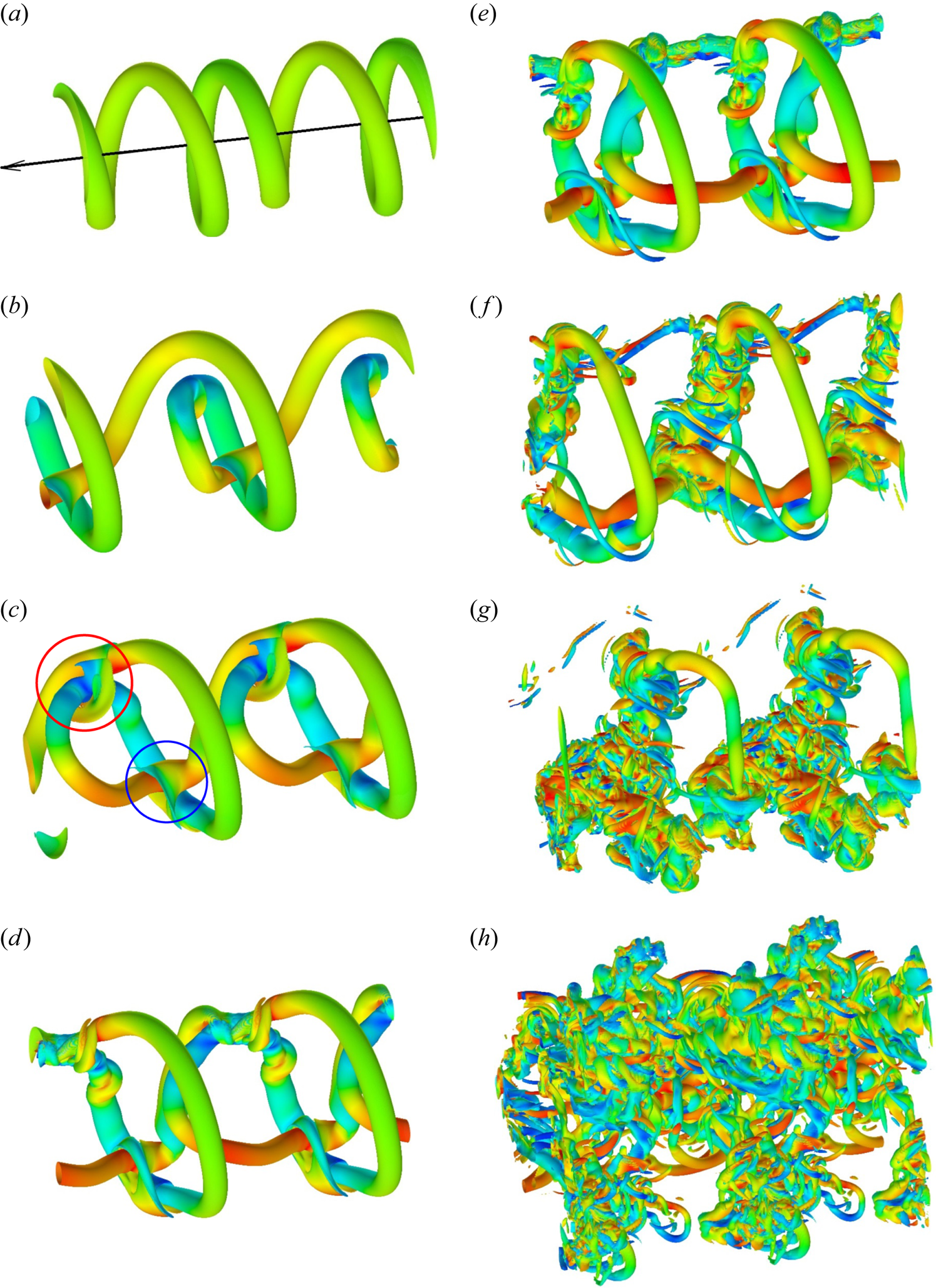
Figure 5. Time evolution of helical vortex with  $L/R=0.2$. The isosurface of the magnitude of vorticity coloured by the axial component of vorticity $\omega _z$. Here $t=$ (a) $8$, (b) $12.5$, (c) $14.75$, (d) $15.5$, (e) $16.13$, (f) $17.38$, (g) $19.25$, (h) $23.38$.
The time evolution of the energy, the enstrophy and the helicity is shown in figure 4. The enstrophy reaches  $\varOmega \approx 420$, which is twice as large as the initial value, at $t=18.5$ when small-scale structures develop. Rapid changes of helicity are observed in figure 4(d). The first change in $16 \lesssim t \lesssim 18$ corresponds to the first reconnection. The second change in $18.8 \lesssim t \lesssim 19.5$ and the third change in $21 \lesssim t \lesssim 22.8$ are also signs of reconnection; in fact, successive reconnections occur, although they become less clear as the flow becomes turbulent.
Figure 6 shows the compensated one-dimensional energy spectrum at two instants after the first reconnection. The velocity field is Fourier transformed in the  $z$ direction and the resulting spectrum is summed up at the regions on the $(r, \theta )$ plane where the rate of dissipation averaged in $z$ is larger than $30\,\%$ of its maximum. It is pointed out that the wavenumber is normalized by the Kolmogorov length $\eta$, while the rate of energy dissipation $\varepsilon$ is used to normalize the compensated energy spectrum. The spectrum shows the Kolmogorov scaling, although the range is narrow at $t=18.25$; it confirms that the flow becomes turbulent after strong interaction of vortices.
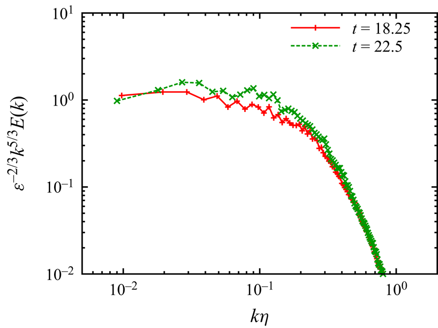
Figure 6. Compensated one-dimensional energy spectrum. Here  $L/R=0.2, t=18.25, 22.5$.
The structure of the vortices are elucidated in figure 7. Here we apply a Gaussian filter to the vorticity as
 \begin{equation} \overline{\omega_i}\left(\boldsymbol{x}\right) = \int G\left(\boldsymbol{x}-\boldsymbol{x'}\right) \omega_i\left(\boldsymbol{x'}\right) {\rm d}\kern 0.06em\boldsymbol{x'}, \quad G\left(\boldsymbol{x}\right) = \left(\frac{6}{{\rm \pi}{\bar{\varDelta}}^2}\right)^{1/2} \exp({-6|\boldsymbol{x}|^2/{\bar{\varDelta}}^2}), \end{equation}
with filter size  ${\bar {\varDelta }}=64\varDelta r_{{min}}$ to remove small-scale structures. The isosurface of the magnitude of the filtered vorticity is shown in figure 7 for $|\boldsymbol {\bar {\omega }}|=0.3\sqrt {\varOmega /R^3}$. It is pointed out that the point and line of sight are different from those in figure 5; they are chosen to clarify the topological change of the vortices. Figure 7 confirms the following: before the first reconnection the helical vortex is deformed but is still connected (figure 7a); the bridges are observed during the reconnection (figure 7b); and vortex rings wrap around the deformed vortex after the reconnection (figure 7c).
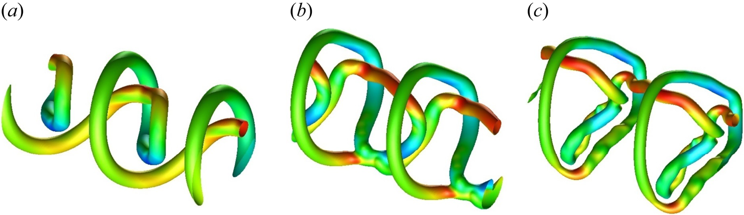
Figure 7. Reconnection process shown by isosurface of magnitude of filtered vorticity. The isosurface is coloured by the axial component of filtered vorticity  $\overline {\omega _z}$. Here $L/R=0.2$, $t=$ (a) $13$, (b) $15.38$, (c) $16.63$.
4. Concluding remarks
The time evolution of the helical vortex disturbed by a long-wave-instability mode has been studied by direct numerical simulation for the two values of the reduced pitch  $L/R=0.2$ and $0.3$. Self-reconnection of the helical vortex plays an important role in both cases. For $L/R=0.3$, a vortex ring detaches from the helical vortex after the reconnection; the pitch of the helical vortex is doubled. For $L/R=0.2$, on the other hand, the vortex ring created after the first reconnection and the remaining helical vortex form a linked system of vortices. The process of reconnection is similar to that observed in Alekseenko et al. (Reference Alekseenko, Kuibin, Shtork, Skripkin and Tsoy2016). However, the present numerical results have clarified the detailed process under perfectly prescribed conditions. More importantly, the long-time evolution after the reconnection has revealed the difference between the two cases: for $L/R=0.2$, the turbulent transition occurs as a consequence of topological constraint, while it does not occur for $L/R=0.3$.
Implication to practical applications is discussed below. In the present work, the Reynolds number is much smaller than that of the helical vortices which occur in wind turbines, while the core size and the pitch are larger. There will be some differences in the process between the two cases. The essential dynamics at least up to the linear regime would be similar because the properties of the long-wave instability do not depend very much on the core size and the Reynolds number; in fact, the process resembling leap-frogging has been observed not only in the present work but also in the experiments (Quaranta et al. Reference Quaranta, Bolnot and Leweke2015). However, the fully nonlinear evolution after the leap-frogging can be different. Vortex tubes should get close within the order of the core size to reconnect. When the core size is small, the vortex tubes will interact and deform in more complex ways than the present results, which may lead to different topology of vortices. Although the topological constraint due to linkage of the vortex tubes is expected to be important also in the helical vortices in wind turbines, the detailed process should be investigated; this is one of the future works, which also include the role of short-wave instabilities (Hattori & Fukumoto Reference Hattori and Fukumoto2009, Reference Hattori and Fukumoto2010, Reference Hattori and Fukumoto2011, Reference Hattori and Fukumoto2012, Reference Hattori and Fukumoto2014; Blanco-Rodríguez & Le Dizès Reference Blanco-Rodríguez and Le Dizès2016, Reference Blanco-Rodríguez and Le Dizès2017; Hattori et al. Reference Hattori, Blanco-Rodríguez and Le Dizès2019) and the effects of torsion (Ricca Reference Ricca1994).
Supplementary movies
Supplementary movies are available at https://doi.org/10.1017/jfm.2024.529.
Funding
This work was supported by JSPS KAKENHI 21H01242. Numerical calculations were performed on AFI-NITY at the Institute of Fluid Science, Tohoku University.
Declaration of interests
The authors report no conflict of interest.


