


Introduction
Salt rejection during sea-ice formation may increase the upper ocean density sufficiently to cause convection, allowing the heat from the waters below to ventilate to the atmosphere. Conversely, a fresh-water flux (e.g. precipitation or ice melt) acts to stabilize the upper ocean. Switching from a thermal mode, where the mixed layer is near the density of the underlying warmer and more saline waters, to a stable, density-stratified mode where little heat is released is largely determined by the regional net fresh-water flux (Reference Martinson, Killworth and GordonMartinson and others, 1981; Reference Martinson, Iannuzzi and JeffriesMartinson and Iannuzzi, 1998). These studies have estimated that, in winter, an ice cover of 30 cm or less can reject enough salt to destabilize the winter water column in part of the central Weddell Sea, Antarctica. This causes deep convection which then releases enough heat from below the ocean mixed layer to completely melt the ice cover. Yet, despite ice growth of this thickness or greater, and continued ice formation in newly formed open-water areas (caused by ice divergence), it is unclear why a large polynya has not been observed since the mid-1970s. Here we present an observed mechanism where snow accumulation on the ice surface and subsequent snow-ice formation provides a fresh-water flux to the ocean in winter, contributing to the stability. This is in contrast to most model formulations (e.g. Reference Martinson, Iannuzzi and JeffriesMartinson and Iannuzzi, 1998) which assume that the flux of snow through ice openings (leads) in winter is negligible.
Slush forms at the upper surface of sea ice when the snow is flooded with brine or sea water. Under cold atmospheric conditions, this slush may then freeze to form snow ice. This flooding depends on the isostatic balance between the weight of the snow and the buoyancy of the underlying ice (Reference Eicken, Lange, Hubberten and WadhamsEicken and others, 1994). Flooding is spatially and temporally variable; ice deformation and snowdrifting result in local variations in isostasy (Reference Wadhams, Lange and AckleyWadhams and others, 1987; Reference Andreas and ClaffeyAndreas and Claffey 1995; Reference Massom, Drinkwater and HaasMassom and others, 1997) as snowdrifts accumulate near ridges or abrupt changes in surface elevation (eg. on thin new ice next to a thicker floe), resulting in ice surfaces both above and below sea level over horizontal distances of a few metres (e.g. Reference Wadhams, Lange and AckleyWadhams and others, 1987; Reference Lytle and AckleyLytle and Ackley, 1996). Estimates of ice surfaces below sea level in the Weddell Sea range from 8% to 40% of the area (Reference Wadhams, Lange and AckleyWadhams and others, 1987; Reference Eicken, Lange, Hubberten and WadhamsEicken and others, 1994). Much of the remaining ice is only slightly (1−2 cm) above sea level (eg. Reference Lange, Schlosser, Ackley, Wadhams and DieckmannLange and others, 1990; Reference Andreas, Lange, Ackley and WadhamsAndreas and others, 1993), so a small addition of snow will cause flooding over a larger area. Despite this ubiquitous negative freeboard, estimates of the contribution of precipitation to the ice mass are relatively low, ranging from 3% to 5% (Reference Lange, Schlosser, Ackley, Wadhams and DieckmannLange and others, 1990; Reference Eicken, Lange, Hubberten and WadhamsEicken and others, 1994). Although these surveys are important for estimating the extent of flooding and snow ice, there are relatively few data (e.g. Reference Lytle and AckleyLytle and Ackley, 1996) available which provide a time series to describe the process of snow-ice formation in the Antarctic sea-ice zone.
This conversion of snow to snow ice makes it difficult to use measurements of snow accumulation to estimate snowfall. Snowfall estimates have been made only by extrapolating measurements from coastal stations (Reference Eicken, Fischer and LemkeEicken and others, 1995), or by calculations of atmospheric moisture transport by data assimilation in global atmospheric models (Reference Budd, Reid and MintyBudd and others, 1995). Early studies (Reference Lange, Schlosser, Ackley, Wadhams and DieckmannLange and others, 1990) had assumed that as the slush freezes, the ice acts as a barrier to brine rejection. More recent studies (e.g. Reference Eicken, Fischer and LemkeEicken and others, 1995; Reference Lytle and AckleyLytle and Ackley, 1996) have, however, indicated that salt rejection to the ocean occurs through the permeable ice during freezing.
Field Data
Salt fluxes to the ocean from a study of snow-ice formation in a newly formed lead are presented here. The data were collected while a vessel (R.V. nathaniel b. palmer) was moored to a drifting pack-ice floe, from 22 to 28 July 1994 at about 67° S, 5° W (Reference McPheeMcPhee and others, 1996). The regional ice concentration was >90%, and a small lead (−10 m by 100 m) appeared on 22 July next to the main ice floe. This open water rapidly froze, and was progressively covered with falling and drifting snow. Ice cores were collected from the frozen lead on 23, 25 and 27 July. The crystal structure was determined by viewing vertical sections between crossed polarizers. The bulk salinity (Si) and oxygen isotope ratio (δi; on cores from 23 and 27 July only) were measured from horizontal sections 1−5 cm thick. Snow pits were examined for vertical profiles of snow density (ps), and snow salinity (ss), and samples were collected for oxygen isotope ratio (δs) measurements. Wind speed and air temperatures were measured either at the lead location or within 200 m (Fig. 1a and b). A vertical rod of thermistors installed in the open water of the lead measured water temperatures every 15 min during the study (Fig. 1c). A stake was frozen in near the thermistor to measure snow accumulation.

Fig. 1. Measured (a) air temperature, (b) wind speed and ( c) ocean temperature (directly beneath the sea ice).
On 24, 25 and 27 July, we measured the snow thickness (hs), ice thickness (h) and the ice draft (bottom of the ice relative to sea level, hd; Table 1) of the lead at 17−24 locations. On 25 July the slush had started to freeze, and the slush thickness (hslush) was also measured. This layer thickness was measured from the top of the newly freezing slush to the top of the solid ice below. Slush was also observed in snow pits on 24 July, but had not formed a coherent, frozen surface, and is included in hs. Gauges (Reference McPhee and UntersteinerMcPhee and Untersteiner, 1982) measured ice melt or growth beneath the thicker ice around the lead. Before and after this experiment, we collected similar data on the regional ice properties.
Table 1. Average ice, snow and slush thickness (in cm) measured over the lead

Model
We calculate the salt transport from measurements of the thickness and bulk properties of the ice and snow. The model is based on simple mass-balance equations and assumes conservation of salt. First, we calculate the fraction of snow (fs) and frozen sea water (fsw) in each of the ice, slush and saline snow layers. Then, using fs, and salinity and thickness data, we calculate the total salt input to the ocean which has occurred since initial ice formation. To calculate fs we assume that it is a linear combination of the isotope value of atmospheric snow (δs) and ice formed from sea water only (δfsw; Reference Jeffries, Shaw, Morris, Veazey and KrouseJeffries and others, 1994):
where the subscript × can be either s or i depending on whether it is a snow-pit or slush sample (both δs) or ice-core (so sample, and
The value of δfsw will depend on the isotopic value of the sea water and the freezing rate of the sea ice. Reference Schlosser, Bayer, Foldvik, Gammelsrod, Rohardt and MunnichSchlosser and others (1989) reported a mean measured isotope value for Weddell Sea winter water of 0.35‰. Reference Lange, Schlosser, Ackley, Wadhams and DieckmannLange and others (1990) use a δfsw of 2‰, while Reference Eicken, Lange, Hubberten and WadhamsEicken and others (1994) use 0.35‰ to calculate a minimum snow content. The average value found for the congelation ice core collected from the lead on 24 July was 1%, and we use this as a representative value. We also calculate the percentage of snow for δfsw = 0‰, to determine the sensitivity of the results to this choice.
The total amount of salt which has been rejected (kg m−2) (to either the ocean or the ice surface, Fice) from sea ice of thickness dhi is :
where sw is the ocean water salinity, pi and ρw are the density of the ice and sea water, respectively, and c is the salt (kg m−3) required to increase the sea-water salinity by l‰. Fice may be negative if highly saline snow freezes to form snow ice. The melting of sea ice can be expressed as a net negative salt (fresh-water) input:
where now dhi is negative. Equations (2a) and (2b) are symmetric only when there is no snow-ice formation (/fsw = 1). In Equation (2a), the salt rejected by ice growth depends on both si and fsw; however, the fresh-water input to the ocean during melting (Equation (2b)) depends only on si The difference in salt input to the ocean between the formation and melt of snow ice is simply the fresh-water input due to the snow.
Upward brine expulsion and frost flowers are common in thin ice types (e.g. Reference Perovich and Richter-MengePerovich and Richter-Menge, 1994; Reference Massom, Drinkwater and HaasMassom and others, 1997). These high-salinity features are later incorporated into the snow cover, with average snow salinities of 8.5‰ and basal snow salinities reaching values up to 54‰. This high-salinity snow is effectively a negative salt flux to the ocean. Flooding of the snow with sea water will also increase the snow salinity, but flooding alone will result in no salt rejection (Fsnow = 0). The equivalent net salt rejection from saline snow, frost flowers or a slush layer is:
where dhs is the thickness of the snow layer. The net ocean salt input since ice formation (Ftotal) is the sum of fice and fsnow.
Assuming a constant flux between sampling times, the average salt flux ![]() can be calculated as the difference in net salt input from one sample to the next (ΔFtotal), divided by the time between samples (Δt):
can be calculated as the difference in net salt input from one sample to the next (ΔFtotal), divided by the time between samples (Δt):
To calculate Fice and Fsnow we first normalize the core and snow-pit data so that they are the same length as the average measured thickness (Table 1). Because of the variation in snow and ice thickness in the lead we believe this is more representative of the average lead than the length of an individual core or depth of an individual snow pit. We then calculate Fice for each core section of length d hi (1−5 cm thick) using the measured si and si values. We assume A = 910 MgnT3. Similarly we calculate Fsnow for each layer of the snow pit using the measured ss, ρs and δs values. The total Fice and Fsnow is simply the sum of all the layers.
We calculate Fice, Fsnow and Ftotal at the four times (23, 24, 25 and 27 July) when thickness data were collected (Table 1). On 23 and 27 July we use the measured ice-core and snow-pit data. For 24 July, we do not have ice-core data (5; and si). To calculate Fice, we assume that the ice is all formed from sea water (/fsw = 1) and has the same average salinity as the columnar ice from the core collected the following day. On 25 July, we do not have isotope values for the ice (si) or slush layers (sb). To calculate Fice we assume that the columnar ice (found beneath the slush layer) is formed only from sea water (/fsw = 1) and has the same average salinity as the columnar ice from the core from 23 July and that the granular ice (found above the slush layer) has about half as much snow content as the ice core collected on 27 July. We use the same ffsw to calculate the contribution of the slush layer to Fsnow. These are conservative estimates of fs, resulting in high estimates of Ftotal for these two days. Although there is a lack of complete data for these two days, and these calculations will have increased uncertainty, it allows us to look at the evolution of Ftotal during the experiment.
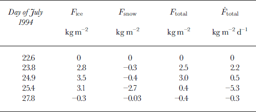
The calculated Fice, Fsnow and Ftotal depend only on the measured bulk properties (s and δ) and on the thickness measurements (Table 1); they do not depend on prior estimates of these properties. Consequently Fice, Fsnow and Ftotal for 23 and 27 July are not affected by these assumptions. We calculate ![]() (Equation (4)) for each of the four time periods during the experiment (Table 2).
(Equation (4)) for each of the four time periods during the experiment (Table 2).
Table 2. Calculated salt input to the ocean from sea-ice formation (fice) wicking into the snow and slush (fsnow) and total salt input ( ftotal) to the ocean since initial ice formation. *** is calculated assuming a constant salt flux from the previous measurement
Results
Ice thickness
Initially, (22 July) cold air temperatures (−24°C) and wind speeds of ∼10 m s− (Fig. 1) caused rapid formation of congelation ice in the lead. The next day, 15 cm of ice was covered by a 4 cm blanket of frost flowers with a salinity of 45‰. By midday on 24 July, air temperatures had warmed ( ∼ −12°C), and increased wind speed (∼20 m s−1; Fig. 1b) caused snowdrifts to form on the thin ice. Flooding was observed from the ship as the snow on the lead darkened from 1630 to 1930 h on 24 July, accompanied by an abrupt increase in all ice temperatures at the thermistor string. In the subsequent cold air temperatures (−10° to −19°C) this flooded snow (slush) froze during the next 2 days (25−27 July). On 27 July, the average thickness of this refreezing slush was 16 cm, slightly more than the more consolidated ice beneath it (Table 1). By late on 24 July basal ice melt was recorded at other locations with thicker (30−40 cm) ice. Although this is not apparent in our crude water-temperature data, increased ocean heat flux is reported during this time by Reference McPheeMcPhee and others (1996). Consequently the ice had probably already started to melt when the thickness measurements were collected on 24 July. The water temperature (Fig. 1c) rapidly increased on 25 July, from −1.8°C to −1.2°C, and remained warmer than −L5°C until 27 July. During these warmer temperatures, ocean heat fluxes as high as 100 W m–2 caused rapid basal ice melt (1.5 cm d−1) (Reference Ackley, Lytle, Kuehn, Golden and DarlingAckley and others, 1995; Reference McPheeMcPhee and others, 1996). Total snow accumulation measured at the stake near the thermistor on 27 July was 25 cm. However, because of the conversion of snow to slush to snow ice in the lead area, the average hs measured there was reduced to 9.7 cm (24 July) and further to an average hs of 4.9 cm (27 July), as reported in Table 1. These average thickness values are plotted in Figure 2 relative to sea level. We have drawn lines between measurement times to provide an indication of the change in location of the interfaces between the snow, ice, slush and snow ice.

Fig. 2. (a) Schematic of transformation from open water to congelation ice to snow ice. the solid arrows and lines are the high-salinity brine rejection, the open arrows are low-salinity melt, and the dotted lines on the arrows are sea-water flooding. although sea-water infiltration is depicted as a vertical process, there was probably also flooding from the side. the marks at the top of the chart indicate times when thickness data were collected. slush thickness on 24 july is estimated from snow-pit data; the remaining thicknesses are from thickness measurements (table 1), (b) cumulative net salt imput to the ocean since the initial ice formation, Ftotal (solid line); salt rejected from ice freezing or melting, fice (dashed line); salt incorporation into the snow cover and slush layer, fsnow (dotted line). positive values are salt input to the ocean; negative values are fresh-water input.
Salinity, oxygen-isotope and ice-textural data
Core salinity on 23 July averaged 11.6 psu (practical salinity units), and in the top 1 cm was 19.5 psu. The crystal structure (Fig. 3) of the ice on 23 July and the high 8, values (0.6−1.5‰) indicated primarily thermodynamic growth (including one rafting event) with little or no snow incorporated. Two cores collected on 27 July were all granular ice, and the 8, values (measured on one core only) were all negative, for a total of fs = 0.74 snow for the entire core (Equation (1)). For δfsw = 0‰, this reduces to fs = 0.71. The core collected on 25 July demonstrated the transition between these two ice types (Fig. 3). It was retrieved in two sections, each 12 cm long with 18 cm of slush between them. The top section was all granular ice, while the bottom section was all columnar ice. The rafting seen in the core from 23 July is not present. Although basal melting may already have started, this is probably indicative of the variation in textural structure across the lead. The average ice salinity decreased only slightly from 11.6 psu on 23 July to 10.6 psu on 27 July.

Fig. 3. Crystal structure and measured 6, of ice cores; depths are relative to the ice surface. δi <1‰ indicates snow ice.
The snow over the new lead ice had an average ss of 18.5 psu or higher. The frost flowers early on and later the brine wicking from the slush further increased the basal snow salinity, with values of 19.5−45 psu. No snow samples, even the thicker snow over the main camp floe, had salinities <0.8psu, indicating that flooding and wicking were also widespread over the thicker ice.
Estimates of salt input to the ocean
On 23 July, after 1.2 days of ice formation, Ftotal was 2.5 kg m−2 (Fig. 3b) with *** = 2 kg m−2 d−1. The small negative Fsnow (−0.3 kg m–2) due to frost-flower formation was about 10% of Ftotal. As the snow accumulation increased the thermal insulation, the ice growth rate slowed and Ftotal increased only slightly over the next 1.1 days to 3.0 kg m–2 on 24 July when Fsnow (−0.4 kg m–2) was about 13% of Ftotal . The flooding of the snow cover and refreezing of this slush resulted in high-salinity brine wicking up into the snow cover. With slush salinities averaging 20‰ and snow salinities averaging 45‰, Fsnow increased to −2.7 kg m–2, almost as much salt (90%) as was rejected in the initial ice growth. With these data, we cannot determine the relative amounts of flooding which occurred vertically through the ice cover and horizontally from the side. However, the high slush and snow salinities relative to fs indicate that some of the flooding must have been high-salinity brine which originated from brine channels or brine pockets within the ice cover. Rapid basal melting caused by high ocean heat fluxes resulted in an increased fresh-water input starting early on 25 July for Ftotal = 0.4 kg m–2 on 25 July. As the basal melt continued, the fresh-water flux eventually negated the previous salt input for a small Ftotal of −0.3 kg m−2 by 27 July. Note that we have assumed no snow has reached the upper ocean to contribute to this fresh-water input. The magnitude of Ftotal on 27 July might be underestimated if, in addition to the original ice cover, some of the snow ice had also melted at the bottom.
Discussions and Conclusions
We calculate a small net fresh-water input to the ocean from the formation of a 26 cm thick ice cover, despite the assumption that no snow or precipitation has reached the upper ocean. This fresh-water input results from high-salinity brine which was incorporated into the snow cover as the ice (or slush) froze. This high-salinity brine rejection occurred during initial ice formation (where about 10% of the total salt was rejected upwards to form frost flowers) and continued as the snow ice formed. Then, as the congelation ice melted, some of this salt remained in the slush and/or snow ice.
Previous formulations suggested that after the initial formation of the relatively thin ice cover, the ocean and atmosphere heat fluxes are such that there is little additional basal sea-ice growth under ice ∼40 cm thick (Reference McPheeMcPhee and others, 1996). This is similar to other studies (e.g. Reference Lange, Schlosser, Ackley, Wadhams and DieckmannLange and others, 1990) where, in equilibrium, the ocean heat flux, the heat flux at the ice or snow surface and the conductive heat flux through the ice determine the ice and snow thickness. In this study, although the total ice thickness remained relatively constant, the ice itself was very dynamic. The high ocean heat fluxes resulted in rapid basal ice melt, reducing the ice thickness; at the same time this basal melt caused surface flooding and snow-ice formation which increased the ice thickness. This process transports the snow (which had originally accumulated on the surface) vertically downward through the ice cover, resulting in an ice cover composed entirely of snow ice after 5 days. Continuing basal melt would have the effect of transporting snow from where it had originally fallen on the ice surface, to the upper ocean, further reducing Ftotal. Model assumptions that precipitation only reaches the upper ocean through open-water regions during winter may not be valid in these circumstances.
This process was not limited to the lead; by 25 July, the thicker sea ice (30−50 cm) nearby had widespread surface flooding. Of 23 cores (total length 11.1m) collected in the region, 30% of the ice volume contained some snow (δi<1‰). For δi <0‰, 22% of the ice volume contained snow. Either of these is a higher percentage on average than reported by other studies (e.g. Reference Lange, Schlosser, Ackley, Wadhams and DieckmannLange and others, 1990; Reference Eicken, Lange, Hubberten and WadhamsEicken and others, 1994). These other studies covered a much larger region of the Weddell Sea, where this high ocean heat flux is not present and similar high rates of basal melt and snow-ice formation are therefore less likely.
The final core (27 July) had measured δi, values which ranged from −25‰ to −9‰ (Fig. 3). It is unusual to find snow ice at the base of an ice core, especially to find δi, as low as 9‰. This basal value is lower than in other cores we collected in the region, and lower than typical values reported by other studies (e.g. Reference Lange, Schlosser, Ackley, Wadhams and DieckmannLange and other, 1990; Reference Eicken, Lange, Hubberten and WadhamsEicken and others, 1994). These low values of δi may have resulted from the rapid snow-ice formation rate and sample collection soon after snow-ice formation. In contrast, it is probable that other cores are typically collected some time after the snow ice has formed. The brine convection which occurs in newly forming sea ice (Reference Eide and MartinEide and Martin, 1975; Reference Niedrauer and MartinNiedrauer and Martin, 1979) may, over time, reduce the evidence of the snow ice, as brine with relatively low δi, values is replaced with brine with higher sea-water isotope values. A reduction in δi values over time might also explain the discrepancy between studies which show a large percentage of flooded snow on the ice surface, yet a relatively small percentage of snow ice in core samples. Future work on the evolution of snow-ice formation is needed to determine if this is typical of newly forming sea ice.
Although the final results from 27 July are largely based on data from two core samples and a few dozen thickness measurements, we do not think it was a unique situation during this time. There is no reason to expect that this lead was any different than others which had formed in the region. During this time period, we observed several instances where snow-covered ice on which we could previously walk turned to slush and we would step through the ice cover. In contrast, several regions which were previously slushy froze solid. It is uncertain, however, how often this type of event occurs.
Salt fluxes ![]() from the new ice varied widely (2 to −5.5 kg m−2 d−1), with positive salt fluxes occurring only during the first 2 days. During the same time, the basal growth and melt rate from the thicker ice (which covered about 90% of the area) varied widely. On average, from 22 to 23 July the thicker ice had a basal melt rate of about 0.5 cm d–1. From 23 to 27 July, basal melt on the thicker floes increased, averaging 1.5 cm d−1. It is difficult to estimate the impact of other processes which were occurring, such as brine drainage, snow-ice formation on the thicker ice, and snow blowing into leads. However, this basal melt on the thicker ice, combined with the fresh-water input from the lead ice, probably resulted in net regional fresh-water flux.
from the new ice varied widely (2 to −5.5 kg m−2 d−1), with positive salt fluxes occurring only during the first 2 days. During the same time, the basal growth and melt rate from the thicker ice (which covered about 90% of the area) varied widely. On average, from 22 to 23 July the thicker ice had a basal melt rate of about 0.5 cm d–1. From 23 to 27 July, basal melt on the thicker floes increased, averaging 1.5 cm d−1. It is difficult to estimate the impact of other processes which were occurring, such as brine drainage, snow-ice formation on the thicker ice, and snow blowing into leads. However, this basal melt on the thicker ice, combined with the fresh-water input from the lead ice, probably resulted in net regional fresh-water flux.
This process of snow-ice formation may provide a stabilizing influence on the ocean by forming an insulating ice cover during periods of ice divergence, without a net ocean salt flux. This process can be sustained only by persistent snowfall which provides the "sponge" for high-salinity brine expulsion and subsequent wicking. As this highly saline snow is flooded and frozen to form snow ice, more snow is required to continue the process. Consequently, deep convection events here could be triggered by atmospheric circulation anomalies, where persistent cold and dry conditions result in sea-ice formation with little snow ice, increasing the total ocean salt flux.
Acknowledgements
We thank the numerous people who helped collect the data including K. Golden, N. Darling, G. Kuehn, J. Evans and the rest of the Antarctic Support Associates crew. J. Ardai and the captain and crew of the nathaniel b. palmer provided excellent logistics support. Thanks also to J.-L. Tison for helpful suggestions. Supported in part by U.S. National Science Foundation grant OPP 93−15934.


