


1 Introduction
A fundamental result in the theory of linear recurrences due to Pólya [Reference PólyaPó21] asserts that if $\{f(n)\}$
is a sequence satisfying a linear recurrence and taking all of its values in the set
$\{f(n)\}$
is a sequence satisfying a linear recurrence and taking all of its values in the set $G\cup \{0\}$
for some finitely generated multiplicative subgroup G of
$G\cup \{0\}$
for some finitely generated multiplicative subgroup G of $\mathbb {Q}^*$
, then the generating series of
$\mathbb {Q}^*$
, then the generating series of $f(n)$
is a finite sum of series of the form
$f(n)$
is a finite sum of series of the form $gx^i/(1-g'x^n)$
with
$gx^i/(1-g'x^n)$
with $g,g'\in G$
and
$g,g'\in G$
and $i,n$
natural numbers along with a finite set of monomials with coefficients in G; moreover, these series can be chosen to have disjoint supports. In particular, Pólya’s theorem gives a complete characterization of sequences
$i,n$
natural numbers along with a finite set of monomials with coefficients in G; moreover, these series can be chosen to have disjoint supports. In particular, Pólya’s theorem gives a complete characterization of sequences $\{f(n)\}\subseteq \mathbb {Q}^*$
that have the property that both
$\{f(n)\}\subseteq \mathbb {Q}^*$
that have the property that both $\{f(n)\}$
and
$\{f(n)\}$
and $\{1/f(n)\}$
satisfy a nontrivial linear recurrence.
$\{1/f(n)\}$
satisfy a nontrivial linear recurrence.
Pólya’s result was later extended to number fields by Benzaghou [Reference BenzaghouBen70] and then by Bézivin [Reference BézivinBé87] to all fields (even those of positive characteristic). A noncommutative multivariate version was recently proved by the authors [Reference Bell and SmertnigBS21]; the noncommutative variant can be interpreted as structural description of unambiguous weighted finite automata over a field.
The generating function of a sequence satisfying a linear recurrence is the power series in some variable x of a rational function about $x=0$
. When one adopts this point of view, it is natural to ask whether such results can be extended to D-finite (or differentiably finite) power series. We recall that if K is a field of characteristic zero, then a univariate power series
$x=0$
. When one adopts this point of view, it is natural to ask whether such results can be extended to D-finite (or differentiably finite) power series. We recall that if K is a field of characteristic zero, then a univariate power series $F(x) =\sum f(n)x^n\in K[[x]]$
is D
-finite if
$F(x) =\sum f(n)x^n\in K[[x]]$
is D
-finite if $F(x)$
satisfies a nontrivial homogeneous linear differential equation with polynomial coefficients:
$F(x)$
satisfies a nontrivial homogeneous linear differential equation with polynomial coefficients:
 $$ \begin{align*}\sum_{i=0}^n p_i(x) F^{(i)}(x)=0,\end{align*} $$
with $p_0(x),\ldots ,p_n(x)\in K[x]$
.
$p_0(x),\ldots ,p_n(x)\in K[x]$
.
Univariate D-finite series were introduced by Stanley [Reference StanleySta80], and the class of D-finite power series is closed under many operations, such as taking K-linear combinations, products, sections, diagonals, Hadamard products, and derivatives, and it contains a multitude of classical generating functions arising from enumerative combinatorics [Reference StanleySta99, Chapter 6]. In particular, algebraic series and their diagonals are D-finite, and a power series F is D-finite if and only if its sequence of coefficients satisfies certain recursions with polynomial coefficients [Reference LipshitzLip89, Theorem 3.7].
Bézivin gave a sweeping extension of Pólya’s result, showing that a univariate D-finite Bézivin series over a field K of characteristic $0$
with the property that there is a fixed
$0$
with the property that there is a fixed $r\ge 1$
and a fixed finitely generated subgroup G of
$r\ge 1$
and a fixed finitely generated subgroup G of $K^*$
such that every coefficient of
$K^*$
such that every coefficient of $F(x)$
can be written as a sum of at most r elements of G is in fact a rational power series and has only simple poles [Reference BézivinBé86].
$F(x)$
can be written as a sum of at most r elements of G is in fact a rational power series and has only simple poles [Reference BézivinBé86].
A natural, and thus far unexplored, direction in which to extend the results of Pólya and Bézivin is to consider multivariate analogues. A multivariate variant of D-finite series was given by Lipshitz [Reference LipshitzLip89]. Here, one has a field K of characteristic zero and declares that a formal multivariate series
is D
-finite if all the partial derivatives $(\partial /\partial x_1)^{e_1} \cdots (\partial /\partial x_d)^{e_d}F$
for
$(\partial /\partial x_1)^{e_1} \cdots (\partial /\partial x_d)^{e_d}F$
for $e_1$
,
$e_1$
, $\ldots \,$
,
$\ldots \,$
, $e_d \ge 0$
are contained in a finite-dimensional vector space over the rational function field
$e_d \ge 0$
are contained in a finite-dimensional vector space over the rational function field $K({\boldsymbol x})$
. Equivalently, for each
$K({\boldsymbol x})$
. Equivalently, for each $i \in [1,d]$
, the series F satisfies a linear partial differential equation of the form
$i \in [1,d]$
, the series F satisfies a linear partial differential equation of the form
 $$\begin{align*}P_{i,n} \cdot (\partial/\partial x_i)^n F + P_{i,n-1} \cdot (\partial/\partial x_i)^{n-1} F + \cdots + P_{i,1} \cdot (\partial/\partial x_i) F + P_{i,0}\cdot F = 0, \end{align*}$$
with polynomials $P_{i,0}$
,
$P_{i,0}$
, $P_{i,1}$
,
$P_{i,1}$
, $\ldots \,$
,
$\ldots \,$
, $P_{i,n} \in K[{\boldsymbol x}]$
, at least one of which is nonzero.
$P_{i,n} \in K[{\boldsymbol x}]$
, at least one of which is nonzero.
In fact, many interesting classical Diophantine questions can be expressed in terms of questions about coefficients of multivariate rational power series and multivariate D-finite series. To give one example, Catalan’s conjecture (now a theorem due to Mihăilescu [Reference MihăilescuMih04]) states that the only solutions to the equation $3^n=2^m+1$
are given by
$3^n=2^m+1$
are given by $(n,m)=(1,1)$
and
$(n,m)=(1,1)$
and $(2,3)$
. This is equivalent to the statement that the bivariate rational power series
$(2,3)$
. This is equivalent to the statement that the bivariate rational power series
 $$ \begin{align*}1/((1-3x_1)(1-x_2))-1/((1-x_1)(1-2x_2)) - 1/((1-x_1)(1-x_2))\end{align*} $$
has nonzero coefficients except for the coefficients of $x_1^2x_2^3$
and
$x_1^2x_2^3$
and $x_1x_2$
. On the other hand, it is typically much more difficult to obtain results about multivariate rational functions and multivariate D-finite series for several reasons. In the case of univariate rational series, the coefficients have a nice closed form and there is a strong structural description of the set of zero coefficients due to Skolem, Mahler, and Lech (see [Reference Everest, van der Poorten, Shparlinski and WardEvdPSW03, Chapter 2.1]). Similarly, for D-finite series, there are many strong results concerning the asymptotics of their coefficients (see [Reference Flajolet and SedgewickFS09], in particular Chapters VII.9 and VIII.7) and one can often make use of these results when considering problems in the univariate case. Straightforward attempts at extending these approaches to higher dimensions typically fail or become too unwieldy. For this reason, new ideas are often important in obtaining multivariate extensions.
$x_1x_2$
. On the other hand, it is typically much more difficult to obtain results about multivariate rational functions and multivariate D-finite series for several reasons. In the case of univariate rational series, the coefficients have a nice closed form and there is a strong structural description of the set of zero coefficients due to Skolem, Mahler, and Lech (see [Reference Everest, van der Poorten, Shparlinski and WardEvdPSW03, Chapter 2.1]). Similarly, for D-finite series, there are many strong results concerning the asymptotics of their coefficients (see [Reference Flajolet and SedgewickFS09], in particular Chapters VII.9 and VIII.7) and one can often make use of these results when considering problems in the univariate case. Straightforward attempts at extending these approaches to higher dimensions typically fail or become too unwieldy. For this reason, new ideas are often important in obtaining multivariate extensions.
It is therefore of considerable interest to understand multivariate D-finite series, although doing so often presents additional technical difficulties. In this paper, we consider structural results for multivariate series that are implied by the additional restrictions on the coefficients of a D-finite series that were imposed by Bézivin and Pólya in the univariate case. For a field K of characteristic zero and a multiplicative subgroup $G \le K^*$
, we set
$G \le K^*$
, we set
and write
for the r-fold sumset of $G_0$
.
$G_0$
.
In view of Bézivin’s and Pólya’s results, we give the following definitions.
Definition 1.1 A power series
![]() is:
is:
-
• a Bézivin series if there exists a finitely generated subgroup $G \le K^*$
and
$r \in \mathbb {N}$
such that
$f(\boldsymbol n) \in rG_0$
for all
$\boldsymbol n \in \mathbb {N}^d$
;
$G \le K^*$
and
$r \in \mathbb {N}$
such that
$f(\boldsymbol n) \in rG_0$
for all
$\boldsymbol n \in \mathbb {N}^d$
; -
• a Pólya series if there exists a finitely generated subgroup
$G \le K^*$
such that
$f(\boldsymbol n) \in G_0$
for all
$\boldsymbol n \in \mathbb {N}^d$
.


The terminology of Pólya series is standard; we have chosen to name Bézivin series based on Bézivin’s results characterizing this type of series in the univariate case [Reference BézivinBé86, Reference BézivinBé87].
In this paper, we completely characterize multivariate D-finite Bézivin and Pólya series. As an immediate consequence, we obtain a characterization of D-finite series whose Hadamard (sub)inverse is also D-finite. The proofs make repeated use of unit equations and results from the theory of semilinear sets.
To state our main result, we recall the notion of semilinear subsets of $\mathbb {N}^d$
. A subset
$\mathbb {N}^d$
. A subset $\mathcal {S} \subseteq \mathbb {N}^d$
is simple linear if it is of the form
$\mathcal {S} \subseteq \mathbb {N}^d$
is simple linear if it is of the form $\mathcal {S} = \boldsymbol a_0 + \boldsymbol a_1\mathbb {N} + \cdots + \boldsymbol a_s \mathbb {N}$
with (
$\mathcal {S} = \boldsymbol a_0 + \boldsymbol a_1\mathbb {N} + \cdots + \boldsymbol a_s \mathbb {N}$
with ( $\mathbb {Z}$
-)linearly independent
$\mathbb {Z}$
-)linearly independent $\boldsymbol a_1$
,
$\boldsymbol a_1$
, $\ldots \,$
,
$\ldots \,$
, $\boldsymbol a_s \in \mathbb {N}^d$
. The terminology comes from the theory of semilinear sets (see Section 2.1). The following is our main result.
$\boldsymbol a_s \in \mathbb {N}^d$
. The terminology comes from the theory of semilinear sets (see Section 2.1). The following is our main result.
Theorem 1.2 Let K be a field of characteristic zero, let $d \ge 0$
, and let
$d \ge 0$
, and let
be a Bézivin series, with all coefficients of F contained in $rG_0$
for some finitely generated subgroup
$rG_0$
for some finitely generated subgroup $G \le K^*$
and
$G \le K^*$
and $r \in \mathbb {N}$
. Then the following statements are equivalent.
$r \in \mathbb {N}$
. Then the following statements are equivalent.
-
(a) F is D-finite.
-
(b) F is rational.
-
(c) F is a (finite) sum of skew-geometric series with coefficients in G, that is, rational functions of the form
where
$$\begin{align*}\frac{g_0u_0}{(1-g_1 u_1)\cdots (1-g_l u_l)}, \end{align*}$$
$u_0$
,
$u_1$
,
$\ldots \,$
,
$u_l$
are monomials in
$x_1$
,
$\ldots \,$
,
$x_d$
such that
$u_1$
,
$\ldots \,$
,
$u_l$
are algebraically independent, and
$g_0$
,
$g_1$
,
$\ldots \,$
,
$g_l \in G$
.
-
(d) As in (c), but in addition, the sum may be taken in such a way that for any two summands, the support is either identical or disjoint. Moreover, every
$\boldsymbol n \in \mathbb {N}^d$
is contained in the support of at most r summands. -
(e) There exists a partition of
$\mathbb {N}^d$
into finitely many simple linear sets so that on each such set
$\mathcal {S}=\boldsymbol a_0 + \boldsymbol a_1 \mathbb {N} + \cdots + \boldsymbol a_s \mathbb {N}$
with
$\boldsymbol a_1$
,
$\ldots \,$
,
$\boldsymbol a_s$
linearly independent, where
$$\begin{align*}f(\boldsymbol a_0 + m_1 \boldsymbol a_1 + \cdots + m_s \boldsymbol a_s) = \sum_{i=1}^l g_{i,0} g_{i,1}^{m_1} \cdots g_{i,s}^{m_s} \qquad\text{for}\ (m_1,\ldots,m_s) \in \mathbb{N}^s, \end{align*}$$
$0 \le l \le r$
and
$g_{i,j} \in G$
for
$i \in [1,l]$
and
$j \in [0,s]$
.


The description of D-finite Pólya series, that is, the case $r=1$
of the previous theorem, deserves separate mention, although it follows readily from the more general result on Bézivin series. Following terminology from formal language theory, a sum of power series
$r=1$
of the previous theorem, deserves separate mention, although it follows readily from the more general result on Bézivin series. Following terminology from formal language theory, a sum of power series $F_1$
,
$F_1$
, $\ldots \,$
,
$\ldots \,$
, $F_n$
is unambiguous if the support of
$F_n$
is unambiguous if the support of $F_i$
is disjoint from the support of
$F_i$
is disjoint from the support of $F_j$
for
$F_j$
for $i \ne j$
(see Definition 3.16).
$i \ne j$
(see Definition 3.16).
Theorem 1.3 Let K be a field of characteristic zero, let $d \ge 0$
, and let
$d \ge 0$
, and let
be a Pólya series with coefficients contained in $G_0$
for some finitely generated subgroup
$G_0$
for some finitely generated subgroup $G \le K^*$
. Then the following statements are equivalent.
$G \le K^*$
. Then the following statements are equivalent.
-
(a) F is D-finite.
-
(b) F is rational.
-
(c) F is a (finite) unambiguous sum of skew-geometric series with coefficients in G.
-
(d) The support of F can be partitioned into finitely many simple linear sets so that on each such set
$\mathcal {S}=\boldsymbol a_0 + \boldsymbol a_1 \mathbb {N} + \cdots + \boldsymbol a_s \mathbb {N}$
with
$\boldsymbol a_1$
,
$\ldots \,$
,
$\boldsymbol a_s$
linearly independent, with
$$\begin{align*}f(\boldsymbol a_0 + m_1 \boldsymbol a_1 + \cdots + m_s \boldsymbol a_s) = g_{0} g_{1}^{m_1} \cdots g_{s}^{m_s} \qquad\text{for}\ (m_1,\ldots,m_s) \in \mathbb{N}^s, \end{align*}$$
$g_{j} \in G$
for
$j \in [0,s]$
.


For a power series
![]() , let
, let
 $$\begin{align*}F^{\dagger} = \sum_{\boldsymbol n \in \mathbb{N}^d} f(\boldsymbol n)^{\dagger} {\boldsymbol x}^{\boldsymbol n}, \end{align*}$$
where $f(\boldsymbol n)^{\dagger } = f(\boldsymbol n)^{-1}$
if
$f(\boldsymbol n)^{\dagger } = f(\boldsymbol n)^{-1}$
if $f(\boldsymbol n)$
is nonzero and
$f(\boldsymbol n)$
is nonzero and $f(\boldsymbol n)^\dagger $
is zero otherwise. The series
$f(\boldsymbol n)^\dagger $
is zero otherwise. The series $F^\dagger $
is the Hadamard subinverse of F.
$F^\dagger $
is the Hadamard subinverse of F.
We call a power series finitary if its coefficients are contained in a finitely generated $\mathbb {Z}$
-subalgebra of K. The set of finitary power series is trivially closed under K-linear combinations, products, sections, diagonals, Hadamard products, and derivatives. Therefore, the set of finitary D-finite series is closed under the same operations. Algebraic series as well as their diagonals and sections are finitary D-finite (see Lemma 7.1).
$\mathbb {Z}$
-subalgebra of K. The set of finitary power series is trivially closed under K-linear combinations, products, sections, diagonals, Hadamard products, and derivatives. Therefore, the set of finitary D-finite series is closed under the same operations. Algebraic series as well as their diagonals and sections are finitary D-finite (see Lemma 7.1).
Corollary 1.4 Let
![]() be finitary D-finite. Then
be finitary D-finite. Then $F^\dagger $
is finitary if and only if F satisfies the equivalent conditions of Theorem 1.3 for some finitely generated subgroup
$F^\dagger $
is finitary if and only if F satisfies the equivalent conditions of Theorem 1.3 for some finitely generated subgroup $G \le K^*$
. In particular, if F and
$G \le K^*$
. In particular, if F and $F^\dagger $
are both finitary D-finite, then they are in fact unambiguous sums of skew-geometric series.
$F^\dagger $
are both finitary D-finite, then they are in fact unambiguous sums of skew-geometric series.
1.1 Notation
Throughout the paper, we fix a field K of characteristic $0$
. When considering a Bézivin series
$0$
. When considering a Bézivin series
![]() , we will always tacitly assume that
, we will always tacitly assume that $G \le K^*$
denotes a finitely generated subgroup, and
$G \le K^*$
denotes a finitely generated subgroup, and $r \ge 1$
denotes a positive integer, such that every coefficient of F is contained in
$r \ge 1$
denotes a positive integer, such that every coefficient of F is contained in $rG_0$
.
$rG_0$
.
2 Preliminaries
For a, $b \in \mathbb {Z}$
, let
$b \in \mathbb {Z}$
, let
![]() . Let
. Let $\mathbb {N} = \{0,1,2,\ldots \}$
and
$\mathbb {N} = \{0,1,2,\ldots \}$
and $\mathbb {N}_{\ge k} = \{\, x \in \mathbb {N} : x \ge k \,\}$
for
$\mathbb {N}_{\ge k} = \{\, x \in \mathbb {N} : x \ge k \,\}$
for $k \in \mathbb {N}$
.
$k \in \mathbb {N}$
.
2.1 Semilinear sets
We summarize a few results from the theory of semilinear sets, and refer to [Reference SakarovitchSak09, Chapter II.7.3] and [Reference D’Alessandro, Intrigila and VarricchioDIV12] for more details.
Definition 2.1 Let $d \ge 1$
. A subset
$d \ge 1$
. A subset $\mathcal {A} \subseteq \mathbb {N}^d$
is:
$\mathcal {A} \subseteq \mathbb {N}^d$
is:
-
• linear if there exist
$\boldsymbol a$
,
$\boldsymbol b_1$
,
$\ldots \,$
,
$\boldsymbol b_l \in \mathbb {N}^d$
such that
$\mathcal {A} = \boldsymbol a + \boldsymbol b_1 \mathbb {N} + \cdots + \boldsymbol b_l \mathbb {N}$
; -
• semilinear if
$\mathcal {A}$
is a finite union of linear sets; -
• simple linear if there exist
$\boldsymbol a$
,
$\boldsymbol b_1$
,
$\ldots \,$
,
$\boldsymbol b_l \in \mathbb {N}^d$
such that
$\mathcal {A} = \boldsymbol a + \boldsymbol b_1 \mathbb {N} + \cdots + \boldsymbol b_l \mathbb {N}$
and
$\boldsymbol b_1$
,
$\ldots \,$
,
$\boldsymbol b_l$
are linearly independent over
$\mathbb {Z}$
.


Whenever we consider a representation of a simple linear set of the form $\boldsymbol a + \boldsymbol b_1 \mathbb {N} + \cdots + \boldsymbol b_l \mathbb {N}$
, we shall tacitly assume that the vectors
$\boldsymbol a + \boldsymbol b_1 \mathbb {N} + \cdots + \boldsymbol b_l \mathbb {N}$
, we shall tacitly assume that the vectors $\boldsymbol b_1$
,
$\boldsymbol b_1$
, $\ldots \,$
,
$\ldots \,$
, $\boldsymbol b_l$
are taken to be linearly independent.
$\boldsymbol b_l$
are taken to be linearly independent.
We make some observations on the uniqueness of the presentation of a linear set $\mathcal {A}$
. Suppose
$\mathcal {A}$
. Suppose $\mathcal {A} = \boldsymbol a + \boldsymbol b_1 \mathbb {N} + \cdots + \boldsymbol b_l \mathbb {N}$
with
$\mathcal {A} = \boldsymbol a + \boldsymbol b_1 \mathbb {N} + \cdots + \boldsymbol b_l \mathbb {N}$
with $\boldsymbol a$
,
$\boldsymbol a$
, $\boldsymbol b_1$
,
$\boldsymbol b_1$
, $\ldots \,$
,
$\ldots \,$
, $\boldsymbol b_l$
as above. The element
$\boldsymbol b_l$
as above. The element $\boldsymbol a$
is uniquely determined by
$\boldsymbol a$
is uniquely determined by $\mathcal {A}$
, as it is the minimum of
$\mathcal {A}$
, as it is the minimum of $\mathcal {A}$
in the coordinatewise partial order on
$\mathcal {A}$
in the coordinatewise partial order on $\mathbb {N}^d$
. Therefore, also the associated monoid
$\mathbb {N}^d$
. Therefore, also the associated monoid $\mathcal {A} - \boldsymbol a \subseteq \mathbb {N}^d$
is uniquely determined by
$\mathcal {A} - \boldsymbol a \subseteq \mathbb {N}^d$
is uniquely determined by $\mathcal {A}$
. The set
$\mathcal {A}$
. The set $\{\boldsymbol b_1,\ldots , \boldsymbol b_l\}$
must contain every atom of
$\{\boldsymbol b_1,\ldots , \boldsymbol b_l\}$
must contain every atom of $\mathcal {A} - \boldsymbol a$
, that is, every element that cannot be written as a sum of two nonzero elements of
$\mathcal {A} - \boldsymbol a$
, that is, every element that cannot be written as a sum of two nonzero elements of $\mathcal {A} - \boldsymbol a$
. If l is taken minimal, then
$\mathcal {A} - \boldsymbol a$
. If l is taken minimal, then $\{\boldsymbol b_1,\ldots ,\boldsymbol b_l\}$
is equal to the set of atoms of
$\{\boldsymbol b_1,\ldots ,\boldsymbol b_l\}$
is equal to the set of atoms of $\mathcal {A} - \boldsymbol a$
, and is therefore unique. In particular, if
$\mathcal {A} - \boldsymbol a$
, and is therefore unique. In particular, if $\mathcal {A}$
is simple linear and
$\mathcal {A}$
is simple linear and $\boldsymbol b_1$
,
$\boldsymbol b_1$
, $\ldots \,$
,
$\ldots \,$
, $\boldsymbol b_l$
are linearly independent, then the representation is unique (up to order of
$\boldsymbol b_l$
are linearly independent, then the representation is unique (up to order of $\boldsymbol b_1$
,
$\boldsymbol b_1$
, $\ldots \,$
,
$\ldots \,$
, $\boldsymbol b_l$
).
$\boldsymbol b_l$
).
If $\mathcal {A}$
and
$\mathcal {A}$
and $\mathcal {A}'$
are two linear sets with the same associated monoid, then there exist
$\mathcal {A}'$
are two linear sets with the same associated monoid, then there exist $\boldsymbol a$
,
$\boldsymbol a$
, $\boldsymbol a'$
,
$\boldsymbol a'$
, $\boldsymbol b_1$
,
$\boldsymbol b_1$
, $\ldots \,$
,
$\ldots \,$
, $\boldsymbol b_l \in \mathbb {N}^d$
with
$\boldsymbol b_l \in \mathbb {N}^d$
with $\mathcal {A} = \boldsymbol a + \boldsymbol b_1 \mathbb {N} + \cdots + \boldsymbol b_l \mathbb {N}$
and
$\mathcal {A} = \boldsymbol a + \boldsymbol b_1 \mathbb {N} + \cdots + \boldsymbol b_l \mathbb {N}$
and $\mathcal {A}'= \boldsymbol a' + \boldsymbol b_1 \mathbb {N} + \cdots + \boldsymbol b_l \mathbb {N}$
. By choosing l minimal, the choice of
$\mathcal {A}'= \boldsymbol a' + \boldsymbol b_1 \mathbb {N} + \cdots + \boldsymbol b_l \mathbb {N}$
. By choosing l minimal, the choice of $\boldsymbol b_1$
,
$\boldsymbol b_1$
, $\ldots \,$
,
$\ldots \,$
, $\boldsymbol b_l$
is again unique (up to order).
$\boldsymbol b_l$
is again unique (up to order).
The semilinear subsets of $\mathbb {N}^d$
are precisely the sets definable in the Presburger arithmetic of
$\mathbb {N}^d$
are precisely the sets definable in the Presburger arithmetic of $\mathbb {N}$
, by a theorem of Ginsburg and Spanier [Reference Ginsburg and SpanierGS66]. We shall make use of the following fundamental (but nontrivial) facts.
$\mathbb {N}$
, by a theorem of Ginsburg and Spanier [Reference Ginsburg and SpanierGS66]. We shall make use of the following fundamental (but nontrivial) facts.
Proposition 2.2 The semilinear subsets of $\mathbb {N}^d$
form a Boolean algebra under set-theoretic intersection and union. In particular, finite unions and finite intersections of semilinear sets, as well as complements of semilinear sets, are again semilinear.
$\mathbb {N}^d$
form a Boolean algebra under set-theoretic intersection and union. In particular, finite unions and finite intersections of semilinear sets, as well as complements of semilinear sets, are again semilinear.
Proof By [Reference SakarovitchSak09, Proposition II.7.15], a subset of $\mathbb {N}^d$
is semilinear if and only if it is rational. By [Reference SakarovitchSak09, Theorem II.7.3], the rational subsets of
$\mathbb {N}^d$
is semilinear if and only if it is rational. By [Reference SakarovitchSak09, Theorem II.7.3], the rational subsets of $\mathbb {N}^d$
form a Boolean algebra.
$\mathbb {N}^d$
form a Boolean algebra.
One can show that every semilinear set is a finite union of simple linear sets. A stronger and much deeper result, which has been shown by Eilenberg and Schützenberger [Reference Eilenberg and SchützenbergerES69] and independently by Ito [Reference ItoIto69], is the following.
Proposition 2.3 Every semilinear set is a finite disjoint union of simple linear sets.
Proof For the proof of Ito, see [Reference ItoIto69, Theorem 2]. Alternatively, one may apply the more general [Reference Eilenberg and SchützenbergerES69, Unambiguity Theorem] of Eilenberg and Schützenberger to the monoid $\mathbb {N}^d$
. This second proof is also contained in the book of Sakarovitch, and one obtains the claim as follows: let
$\mathbb {N}^d$
. This second proof is also contained in the book of Sakarovitch, and one obtains the claim as follows: let $S \subseteq \mathbb {N}^d$
be semilinear. Then S is a rational subset of
$S \subseteq \mathbb {N}^d$
be semilinear. Then S is a rational subset of $\mathbb {N}^d$
(see [Reference SakarovitchSak09, Proposition II.7.5] and the discussion preceding it). By [Reference SakarovitchSak09, Theorem II.7.4] or [Reference Eilenberg and SchützenbergerES69, Unambiguity Theorem], every rational subset of
$\mathbb {N}^d$
(see [Reference SakarovitchSak09, Proposition II.7.5] and the discussion preceding it). By [Reference SakarovitchSak09, Theorem II.7.4] or [Reference Eilenberg and SchützenbergerES69, Unambiguity Theorem], every rational subset of $\mathbb {N}^d$
is unambiguous. Again by [Reference SakarovitchSak09, Proposition II.7.15], every unambiguous rational subset of
$\mathbb {N}^d$
is unambiguous. Again by [Reference SakarovitchSak09, Proposition II.7.15], every unambiguous rational subset of $\mathbb {N}^d$
is a finite disjoint union of simple linear sets.
$\mathbb {N}^d$
is a finite disjoint union of simple linear sets.
2.2 Unit equations
Unit equations play a central role in our proofs. We recall the fundamental finiteness result. For number fields, it was proved independently by Evertse [Reference EvertseEve84] and van der Poorten and Schlickewei [Reference van der Poorten and SchlickeweivdPS82]; the extension to arbitrary fields appears in [Reference van der Poorten and SchlickeweivdPS91]. We refer to [Reference Evertse and GyőryEG15, Chapter 6] or [Reference Bombieri and GublerBG06, Theorem 7.4.1] for more details.
Let G be a finitely generated subgroup of the multiplicative subgroup $K^*$
of the field K. It is important here that
$K^*$
of the field K. It is important here that $\operatorname {\mathrm {char}} K=0$
. Let
$\operatorname {\mathrm {char}} K=0$
. Let $m \ge 1$
. A solution
$m \ge 1$
. A solution $(x_1,\ldots ,x_m) \in K^{m}$
to an equation of the form
$(x_1,\ldots ,x_m) \in K^{m}$
to an equation of the form
 $$ \begin{align} X_1 + \cdots + X_m = 0 \end{align} $$
is nondegenerate if $\sum _{i \in I} x_i \ne 0$
for every
$\sum _{i \in I} x_i \ne 0$
for every $\emptyset \subsetneq I \subsetneq [1,m]$
. In particular, if
$\emptyset \subsetneq I \subsetneq [1,m]$
. In particular, if $m \ge 2$
, then all
$m \ge 2$
, then all $x_i$
of a nondegenerate solution are nonzero.
$x_i$
of a nondegenerate solution are nonzero.
Proposition 2.4 (Evertse; van der Poorten and Schlickewei)
There exist only finitely many projective points $(x_1: \cdots : x_m)$
with coordinates
$(x_1: \cdots : x_m)$
with coordinates $x_1$
,
$x_1$
, $\ldots \,$
,
$\ldots \,$
, $x_m \in G$
such that
$x_m \in G$
such that $(x_1,\ldots ,x_m)$
is a nondegenerate solution to the unit equation (2.1).
$(x_1,\ldots ,x_m)$
is a nondegenerate solution to the unit equation (2.1).
It is easily seen that there can be infinitely many degenerate solutions (even when considered as projective points), but one can recursively apply the theorem to subequations. In particular, we will commonly use an argument of the following type.
Let $\Omega $
be some index set, and let
$\Omega $
be some index set, and let $g_1$
,
$g_1$
, $\ldots \,$
,
$\ldots \,$
, $g_m \colon \Omega \to G_0$
be maps such that
$g_m \colon \Omega \to G_0$
be maps such that
 $$\begin{align*}g_1(\omega) + \cdots + g_m(\omega) = 0 \qquad\text{for}\ \omega \in \Omega. \end{align*}$$
For every partition $\mathcal {P} = \{I_1,\ldots ,I_t\}$
of the set
$\mathcal {P} = \{I_1,\ldots ,I_t\}$
of the set $[1,m]$
, let
$[1,m]$
, let $\Omega _{\mathcal {P}} \subseteq \Omega $
consist of all
$\Omega _{\mathcal {P}} \subseteq \Omega $
consist of all $\omega $
such that for all
$\omega $
such that for all $j \in [1,t]$
, the tuple
$j \in [1,t]$
, the tuple $(g_i(\omega ))_{i \in I_j}$
is a nondegenerate solution of the unit equation
$(g_i(\omega ))_{i \in I_j}$
is a nondegenerate solution of the unit equation $\sum _{i \in I_j} X_i = 0$
. Since every solution of a unit equation can be partitioned into nondegenerate solutions in at least one way, we obtain
$\sum _{i \in I_j} X_i = 0$
. Since every solution of a unit equation can be partitioned into nondegenerate solutions in at least one way, we obtain $\Omega = \bigcup _{\mathcal {P}} \Omega _{\mathcal {P}}$
, where the union runs over all partitions of
$\Omega = \bigcup _{\mathcal {P}} \Omega _{\mathcal {P}}$
, where the union runs over all partitions of $[1,m]$
.
$[1,m]$
.
Since there are only finitely many partitions of $[1,m]$
, one can often deal with each
$[1,m]$
, one can often deal with each $\Omega _{\mathcal {P}}$
separately, or reduce to one
$\Omega _{\mathcal {P}}$
separately, or reduce to one $\Omega _{\mathcal {P}}$
having some desirable property by an application of the pigeonhole principle. For example, if
$\Omega _{\mathcal {P}}$
having some desirable property by an application of the pigeonhole principle. For example, if $\Omega $
is infinite, then at least one
$\Omega $
is infinite, then at least one $\Omega _{\mathcal {P}}$
is infinite. Similarly, if
$\Omega _{\mathcal {P}}$
is infinite. Similarly, if $\Omega = \mathbb {N}^d$
, then not all
$\Omega = \mathbb {N}^d$
, then not all $\Omega _{\mathcal {P}}$
can be contained in semilinear sets of rank at most
$\Omega _{\mathcal {P}}$
can be contained in semilinear sets of rank at most $d-1$
, because
$d-1$
, because $\mathbb {N}^d$
cannot be covered by finitely many semilinear sets of rank
$\mathbb {N}^d$
cannot be covered by finitely many semilinear sets of rank $\le d-1$
.
$\le d-1$
.
2.3 Hahn series
We recall that an abelian group G is totally ordered as a group if G is equipped with a total order $\le $
with the property that
$\le $
with the property that $a+c\le b+c$
whenever
$a+c\le b+c$
whenever $a,b, c\in G$
are such that
$a,b, c\in G$
are such that $a\le b$
. For the group
$a\le b$
. For the group $H=\mathbb {Q}^d$
, we will give H a total ordering that is compatible with the group structure by first picking positive linearly independent real numbers
$H=\mathbb {Q}^d$
, we will give H a total ordering that is compatible with the group structure by first picking positive linearly independent real numbers $\epsilon _1$
,
$\epsilon _1$
, $\ldots \,$
,
$\ldots \,$
, $\epsilon _d$
and then declaring that
$\epsilon _d$
and then declaring that $(a_1,\ldots , a_d)\le (b_1,\ldots ,b_d)$
if and only if
$(a_1,\ldots , a_d)\le (b_1,\ldots ,b_d)$
if and only if
 $$\begin{align*}\sum_{i=1}^d a_i \epsilon_i \le \sum_{i=1}^d b_i \epsilon_i. \end{align*}$$
Lemma 2.5 The following hold for the above order:
-
•
$\mathbb {N}^d$
is a well-ordered subset of
$\mathbb {Q}^d$
. -
• If
$(a_1,\ldots , a_d)< (b_1,\ldots ,b_d)$
and if
$(c_1,\ldots ,c_d)\in \mathbb {Q}^d$
, then there is some
$N>0$
such that
$n(b_1,\ldots ,b_d)> n(a_1,\ldots ,a_d)+(c_1,\ldots ,c_d)$
whenever
$n\ge N$
.


Proof Let S be a nonempty subset of $\mathbb {N}^d$
. Pick
$\mathbb {N}^d$
. Pick $(a_1,\ldots ,a_d)\in S$
, and let
$(a_1,\ldots ,a_d)\in S$
, and let
![]() . Then, if
. Then, if $(b_1,\ldots , b_d)\in S$
is less than
$(b_1,\ldots , b_d)\in S$
is less than $(a_1,\ldots ,a_d)$
, we must have
$(a_1,\ldots ,a_d)$
, we must have $b_i \le u/\epsilon _i$
for
$b_i \le u/\epsilon _i$
for $i \in [1,d]$
. Thus, there are only finitely many elements in S that are less than u and so S has a smallest element. Next, if
$i \in [1,d]$
. Thus, there are only finitely many elements in S that are less than u and so S has a smallest element. Next, if $(a_1,\ldots , a_d)< (b_1,\ldots ,b_d)$
, then
$(a_1,\ldots , a_d)< (b_1,\ldots ,b_d)$
, then
![]() . Then
. Then $n\theta> \sum _{i=1}^d c_i \epsilon _i$
for all n sufficiently large.
$n\theta> \sum _{i=1}^d c_i \epsilon _i$
for all n sufficiently large.
The second property is equivalent to $\mathbb {Q}^d$
with the given order being archimedean.
$\mathbb {Q}^d$
with the given order being archimedean.
If G is a totally ordered abelian group, we can define the ring of Hahn power series

Then $K(\mkern -3mu( {\boldsymbol x}^G)\mkern -3mu)$
, together with the obvious operations, is a ring. For
$K(\mkern -3mu( {\boldsymbol x}^G)\mkern -3mu)$
, together with the obvious operations, is a ring. For
 $$\begin{align*}F = \sum_{g\in G} a_g {\boldsymbol x}^g \in K(\mkern-3mu( {\boldsymbol x}^G )\mkern-3mu), \end{align*}$$
one defines
to be the support of F. We define
. Then there is a valuation $\mathsf v \colon K(\mkern -3mu( x^G )\mkern -3mu) \to G \cup \{\infty \}$
, defined as follows: one sets
$\mathsf v \colon K(\mkern -3mu( x^G )\mkern -3mu) \to G \cup \{\infty \}$
, defined as follows: one sets $\mathsf v(F)=g$
where
$\mathsf v(F)=g$
where ${\boldsymbol x}^g$
is the minimal monomial in the support of F if
${\boldsymbol x}^g$
is the minimal monomial in the support of F if $F \ne 0$
, and
$F \ne 0$
, and $\mathsf v(0)=\infty $
.
$\mathsf v(0)=\infty $
.
For $F_1 = \sum _{g\in G} a_g {\boldsymbol x}^g$
and
$F_1 = \sum _{g\in G} a_g {\boldsymbol x}^g$
and $F_2 = \sum _{g \in G} b_g {\boldsymbol x}^g \in K(\mkern -3mu( {\boldsymbol x}^G )\mkern -3mu)$
, the Hadamard product is defined as
$F_2 = \sum _{g \in G} b_g {\boldsymbol x}^g \in K(\mkern -3mu( {\boldsymbol x}^G )\mkern -3mu)$
, the Hadamard product is defined as
 $$\begin{align*}F_1 \odot F_2 = \sum_{g \in G} a_g b_g {\boldsymbol x}^g. \end{align*}$$
If K is algebraically closed and G is divisible, then $K(\mkern -3mu( {\boldsymbol x}^G)\mkern -3mu)$
is an algebraically closed field. In particular, if we use the order given above for
$K(\mkern -3mu( {\boldsymbol x}^G)\mkern -3mu)$
is an algebraically closed field. In particular, if we use the order given above for $H=\mathbb {Q}^d$
, we see that if K is algebraically closed, then
$H=\mathbb {Q}^d$
, we see that if K is algebraically closed, then $K(\mkern -3mu( {\boldsymbol x}^H)\mkern -3mu)$
is algebraically closed. After making the identification
$K(\mkern -3mu( {\boldsymbol x}^H)\mkern -3mu)$
is algebraically closed. After making the identification
![]() , where
, where $\boldsymbol e_i=(0,\ldots ,1,\ldots ,0)$
and where there is a
$\boldsymbol e_i=(0,\ldots ,1,\ldots ,0)$
and where there is a $1$
in the ith coordinate and zeros in all other coordinates, we have that the formal power series ring
$1$
in the ith coordinate and zeros in all other coordinates, we have that the formal power series ring
![]() is a subalgebra of
is a subalgebra of $K(\mkern -3mu( x^H)\mkern -3mu)$
.
$K(\mkern -3mu( x^H)\mkern -3mu)$
.
We will find it convenient to write ${\boldsymbol x}^{(a_1,\ldots ,a_d)} =x_1^{a_1}\cdots x_d^{a_d}$
and write
${\boldsymbol x}^{(a_1,\ldots ,a_d)} =x_1^{a_1}\cdots x_d^{a_d}$
and write $K(\mkern -3mu( x_1^{\mathbb {Q}},\ldots ,x_{d}^{\mathbb {Q}} )\mkern -3mu)$
for
$K(\mkern -3mu( x_1^{\mathbb {Q}},\ldots ,x_{d}^{\mathbb {Q}} )\mkern -3mu)$
for $K(\mkern -3mu( {\boldsymbol x}^H)\mkern -3mu)$
. In the other direction, we will find it convenient to abbreviate the power series ring as
$K(\mkern -3mu( {\boldsymbol x}^H)\mkern -3mu)$
. In the other direction, we will find it convenient to abbreviate the power series ring as
![]() . These conventions are consistent with usual multi-index notation, and so for
. These conventions are consistent with usual multi-index notation, and so for $\boldsymbol a= (a_1,\ldots ,a_d)$
and
$\boldsymbol a= (a_1,\ldots ,a_d)$
and $\boldsymbol b = (b_1,\ldots ,b_d) \in \mathbb {Q}^d$
, we write
$\boldsymbol b = (b_1,\ldots ,b_d) \in \mathbb {Q}^d$
, we write $\boldsymbol a + \boldsymbol b = (a_1+b_1, \ldots , a_d + b_d)$
and
$\boldsymbol a + \boldsymbol b = (a_1+b_1, \ldots , a_d + b_d)$
and $\boldsymbol a \boldsymbol b = (a_1b_1, \ldots , a_d b_d)$
. If
$\boldsymbol a \boldsymbol b = (a_1b_1, \ldots , a_d b_d)$
. If $\boldsymbol a \in \mathbb {Z}^d$
and
$\boldsymbol a \in \mathbb {Z}^d$
and ${\boldsymbol \lambda }=(\lambda _1,\ldots ,\lambda _d)$
with
${\boldsymbol \lambda }=(\lambda _1,\ldots ,\lambda _d)$
with $\lambda _i \in K(\mkern -3mu( \boldsymbol x^{H} )\mkern -3mu)$
, we also write
$\lambda _i \in K(\mkern -3mu( \boldsymbol x^{H} )\mkern -3mu)$
, we also write ${\boldsymbol \lambda }^{\boldsymbol a}= \prod _{i=1}^d \lambda _i^{a_i}$
, although we will usually only use this for
${\boldsymbol \lambda }^{\boldsymbol a}= \prod _{i=1}^d \lambda _i^{a_i}$
, although we will usually only use this for $\lambda _i \in K^*$
or
$\lambda _i \in K^*$
or $\lambda _i$
a monomial.
$\lambda _i$
a monomial.
The set of [rational] Bézivin series is not closed under products or differentiation. However, it is closed under Hadamard products and it forms a $K[{\boldsymbol x}]$
-submodule of
$K[{\boldsymbol x}]$
-submodule of
![]() , as the following easy lemma shows.
, as the following easy lemma shows.
Lemma 2.6 Let
![]() be a Bézivin series with coefficients in
be a Bézivin series with coefficients in $rG_0$
. If
$rG_0$
. If $P \in K[\boldsymbol x]$
is a polynomial with s terms in its support, then there exists a set
$P \in K[\boldsymbol x]$
is a polynomial with s terms in its support, then there exists a set $B \subseteq K$
of cardinality
$B \subseteq K$
of cardinality $rs$
such that
$rs$
such that
 $$\begin{align*}[{\boldsymbol x}^{\boldsymbol n}] FP \in BG_0 = \sum_{b \in B} bG_0\qquad\text{for}\ \boldsymbol n \in \mathbb{N}^d. \end{align*}$$
In particular, the series $PF$
is a Bézivin series with coefficients in
$PF$
is a Bézivin series with coefficients in $rsG_0'$
for a suitable finitely generated subgroup
$rsG_0'$
for a suitable finitely generated subgroup $G' \le K^*$
.
$G' \le K^*$
.
We will need to understand the factorization of polynomials of the form $1-c{\boldsymbol x}^{\boldsymbol e}$
with
$1-c{\boldsymbol x}^{\boldsymbol e}$
with $\boldsymbol e \in \mathbb {N}^d$
.
$\boldsymbol e \in \mathbb {N}^d$
.
Lemma 2.7 Let K be algebraically closed, and let $\boldsymbol e = (e_1,\ldots ,e_d) \in \mathbb {Z}^d \setminus \{\boldsymbol 0\}$
. In the factorial domain
$\boldsymbol e = (e_1,\ldots ,e_d) \in \mathbb {Z}^d \setminus \{\boldsymbol 0\}$
. In the factorial domain $K[{\boldsymbol x}^{\pm 1}]=K[x_1^{\pm 1},\ldots ,x_d^{\pm 1}]$
, the Laurent polynomial
$K[{\boldsymbol x}^{\pm 1}]=K[x_1^{\pm 1},\ldots ,x_d^{\pm 1}]$
, the Laurent polynomial
 $$\begin{align*}Q = 1 - c {\boldsymbol x}^{\boldsymbol e} \qquad\text{with}\ c \in K^* \end{align*}$$
factors into irreducibles as
 $$\begin{align*}Q = \prod_{j=1}^t (1 - \zeta^j b {\boldsymbol x}^{\boldsymbol e/t}), \end{align*}$$
where $t=\gcd (e_1,\ldots ,e_d)$
,
$t=\gcd (e_1,\ldots ,e_d)$
, $\zeta \in K^*$
is a primitive t-th root of unity, and
$\zeta \in K^*$
is a primitive t-th root of unity, and $b^t=c$
. In particular, the Laurent polynomial Q is irreducible if and only if
$b^t=c$
. In particular, the Laurent polynomial Q is irreducible if and only if $\gcd (e_1,\ldots ,e_d) = 1$
.
$\gcd (e_1,\ldots ,e_d) = 1$
.
Proof The proof follows an argument of Ostrowski [Reference OstrowskiOst76, Theorem IX]. Since $(e_1/t, \ldots , e_d/t)$
is a unimodular row, there exists a matrix
$(e_1/t, \ldots , e_d/t)$
is a unimodular row, there exists a matrix $A=(a_{i,j})_{i,j \in [1,d]} \in \operatorname {\mathrm {GL}}_d(\mathbb {Z})$
whose first row is
$A=(a_{i,j})_{i,j \in [1,d]} \in \operatorname {\mathrm {GL}}_d(\mathbb {Z})$
whose first row is $(e_1/t, \ldots , e_d/t)$
. This matrix A induces a ring automorphism
$(e_1/t, \ldots , e_d/t)$
. This matrix A induces a ring automorphism $\varphi $
of the Laurent polynomial ring
$\varphi $
of the Laurent polynomial ring $K[{\boldsymbol x}^{\pm 1}]$
with
$K[{\boldsymbol x}^{\pm 1}]$
with $\varphi (x_i)=\prod _{j=1}^d x_j^{a_{i,j}}$
. Then
$\varphi (x_i)=\prod _{j=1}^d x_j^{a_{i,j}}$
. Then $\varphi ^{-1}(Q) = 1-cx_1^{t}$
. Since
$\varphi ^{-1}(Q) = 1-cx_1^{t}$
. Since $K[x_1^{\pm 1}]$
is divisor-closed in
$K[x_1^{\pm 1}]$
is divisor-closed in $K[{\boldsymbol x}^{\pm 1}]$
, the problem reduces to that of factoring the univariate Laurent polynomial
$K[{\boldsymbol x}^{\pm 1}]$
, the problem reduces to that of factoring the univariate Laurent polynomial $1-cx_1^{t}$
in
$1-cx_1^{t}$
in $K[x_1^{\pm 1}]$
. Since
$K[x_1^{\pm 1}]$
. Since $K[x_1^{\pm 1}]$
is obtained from the factorial domain
$K[x_1^{\pm 1}]$
is obtained from the factorial domain $K[x_1]$
by inverting the prime element
$K[x_1]$
by inverting the prime element $x_1$
, and clearly
$x_1$
, and clearly $x_1$
is not a factor of
$x_1$
is not a factor of $1-cx_1^t$
in
$1-cx_1^t$
in $K[x_1]$
, it suffices to consider the factorization of
$K[x_1]$
, it suffices to consider the factorization of $1-cx_1^t$
in
$1-cx_1^t$
in $K[x_1]$
. However, here the result is clear.
$K[x_1]$
. However, here the result is clear.
3 Rational series with polynomial–exponential coefficients
In this section, we consider rational series whose denominator is a product of elements of the form $1-cu$
with
$1-cu$
with $c \in K^*$
and
$c \in K^*$
and $u \in K[{\boldsymbol x}]$
a nonconstant monomial. This will come in handy in the later sections, as it will turn out that rational Bézivin series are always of such a form. For the class of rational series under investigation here, it is possible to give a fairly explicit structural description of their coefficient sequences, namely they are piecewise polynomial–exponential on simple linear subsets of
$u \in K[{\boldsymbol x}]$
a nonconstant monomial. This will come in handy in the later sections, as it will turn out that rational Bézivin series are always of such a form. For the class of rational series under investigation here, it is possible to give a fairly explicit structural description of their coefficient sequences, namely they are piecewise polynomial–exponential on simple linear subsets of $\mathbb {N}^d$
.
$\mathbb {N}^d$
.
Definition 3.1 Let $f \colon \mathbb {N}^d \to K$
be a sequence.
$f \colon \mathbb {N}^d \to K$
be a sequence.
-
• The sequence f is piecewise polynomial–exponential on simple linear subsets of
$\mathbb {N}^d$
if there exists a partition of
$\mathbb {N}^d$
into simple linear sets
$\mathcal {S}_1$
,
$\ldots \,$
,
$\mathcal {S}_m$
so that for each
$i \in [1,m]$
, there exist
$k_i \in \mathbb {N}$
, polynomials
$A_{i,1}$
,
$\ldots \,$
,
$A_{i,k_i} \in K[{\boldsymbol x}]$
, and
${\boldsymbol \alpha }_{i,1}$
,
$\ldots \,$
,
${\boldsymbol \alpha }_{i,k_i} \in (K^*)^d$
such that
$$\begin{align*}f({\boldsymbol n}) = \sum_{j = 1}^{k_i} A_{i,j}(\boldsymbol n) {\boldsymbol\alpha}_{i,j}^{\boldsymbol n} \qquad\text{for}\ {\boldsymbol n} \in \mathcal{S}_i. \end{align*}$$
-
• The sequence f is piecewise polynomial on simple linear subsets of
$\mathbb {N}^d$
if one can moreover take
${\boldsymbol \alpha }_{i,j}=(1,\ldots ,1)$
for all
$i \in [1,m]$
and
$j \in [1,k_i]$
. -
• The sequence f is piecewise exponential on simple linear subsets of
$\mathbb {N}^d$
if one can take the polynomials
$A_{i,j}$
to be constant for all
$i \in [1,m]$
and
$j \in [1,k_i]$
.


Note that in the piecewise exponential case, sums of exponentials ( $k_i> 1$
) are allowed. There is no restriction on the ranks of the simple linear sets; the rank of
$k_i> 1$
) are allowed. There is no restriction on the ranks of the simple linear sets; the rank of $\mathcal {S}_i$
may be smaller than d, and also need not be the same for
$\mathcal {S}_i$
may be smaller than d, and also need not be the same for $\mathcal {S}_1$
,
$\mathcal {S}_1$
, $\ldots \,$
,
$\ldots \,$
, $\mathcal {S}_m$
. Each of these three types of representation is trivially preserved under refinements of the partition. In particular, representations of the above types are not unique. It is not hard to see that every series
$\mathcal {S}_m$
. Each of these three types of representation is trivially preserved under refinements of the partition. In particular, representations of the above types are not unique. It is not hard to see that every series
![]() , whose coefficient sequence is polynomial–exponential on simple subsets of
, whose coefficient sequence is polynomial–exponential on simple subsets of $\mathbb {N}^d$
, is rational (see Corollary 3.12). We give an easy example to illustrate the definition.
$\mathbb {N}^d$
, is rational (see Corollary 3.12). We give an easy example to illustrate the definition.
Example 3.2 Consider the sequence $f \colon \mathbb {N}^2 \to \mathbb {Q}$
defined by
$f \colon \mathbb {N}^2 \to \mathbb {Q}$
defined by
 $$\begin{align*}\begin{aligned} \sum_{m,n =0}^\infty f(m,n)x^my^n &= \frac{1}{1-2xy} + \frac{1}{1-3xy} + \frac{y}{(1-3xy)^2(1-5y)} + \frac{x}{(1-xy)(1-x)} \\ &= \sum_{k=0}^\infty (2^k+3^k)x^ky^k + \sum_{k,l=0}^\infty (k+1)3^k5^lx^ky^{k+l+1} + \sum_{k,l=0}^\infty x^{k+l+1}y^{l}. \end{aligned} \end{align*}$$
Then
 $$\begin{align*}f(m,n) = \begin{cases} 2^m + 3^m, & \text{if}\ m=n, \\ \frac{1}{5} (m+1)(\frac{3}{5})^m 5^n, & \text{if}\ m < n, \\ 1, & \text{if}\ m>n. \end{cases} \end{align*}$$
Since
 $$\begin{align*}\begin{aligned} \{\, (n,n) \in \mathbb{N}^2 : n \in \mathbb{N} \,\} &= (1,1)\mathbb{N},\\ \{\, (m,n) \in \mathbb{N}^2 : m < n \,\} &= (0,1) + (1,1)\mathbb{N} + (0,1)\mathbb{N}, \text{ and }\\ \{\, (m,n) \in \mathbb{N}^2 : m> n \,\} &= (1,0) + (1,1)\mathbb{N} + (1,0)\mathbb{N} \end{aligned} \end{align*}$$
are simple linear sets, the sequence f is piecewise polynomial–exponential on simple linear subsets of $\mathbb {N}^2$
. However, f is neither piecewise polynomial nor piecewise exponential on simple linear subsets of
$\mathbb {N}^2$
. However, f is neither piecewise polynomial nor piecewise exponential on simple linear subsets of $\mathbb {N}^2$
. The coefficient sequence of
$\mathbb {N}^2$
. The coefficient sequence of $\frac {1}{1-2xy} + \frac {1}{1-3xy}$
is piecewise exponential on simple linear subsets of
$\frac {1}{1-2xy} + \frac {1}{1-3xy}$
is piecewise exponential on simple linear subsets of $\mathbb {N}^2$
, and the coefficient sequence of
$\mathbb {N}^2$
, and the coefficient sequence of $\frac {x}{(1-xy)(1-x)}$
is piecewise polynomial on simple linear subsets of
$\frac {x}{(1-xy)(1-x)}$
is piecewise polynomial on simple linear subsets of $\mathbb {N}^2$
.
$\mathbb {N}^2$
.
The following basic properties hold.
Lemma 3.3 Let $\mathcal {PE}$
,
$\mathcal {PE}$
, $\mathcal {P}$
,
$\mathcal {P}$
,
![]() denote, respectively, the power series whose coefficient sequences are piecewise polynomial–exponential [polynomial, exponential] on simple linear subsets of
denote, respectively, the power series whose coefficient sequences are piecewise polynomial–exponential [polynomial, exponential] on simple linear subsets of $\mathbb {N}^d$
.
$\mathbb {N}^d$
.
-
(1) Each of
$\mathcal {PE}$
,
$\mathcal {P}$
, and
$\mathcal E$
is a
$K[\boldsymbol x]$
-submodule of
and is closed under Hadamard products. -
(2) The sets
$\mathcal {PE}$
and
$\mathcal {P}$
are also closed under products and partial derivatives. In particular,
$\mathcal {PE}$
and
$\mathcal {P}$
form subalgebras of
.


Proof
(1) Let F and G be series that are [polynomial–exponential, polynomial, exponential] on simple linear subsets. It is clear that for every monomial u and every scalar $\lambda \in K$
, also
$\lambda \in K$
, also $\lambda uF$
is of the same form. Thus, it suffices to show that the same is true for
$\lambda uF$
is of the same form. Thus, it suffices to show that the same is true for $F+G$
. If
$F+G$
. If $\mathcal {S}$
and
$\mathcal {S}$
and $\mathcal {T} \subseteq \mathbb {N}^d$
are simple linear subsets, then the intersection
$\mathcal {T} \subseteq \mathbb {N}^d$
are simple linear subsets, then the intersection $\mathcal {S} \cap \mathcal {T}$
is semilinear. By Proposition 2.3, the intersection
$\mathcal {S} \cap \mathcal {T}$
is semilinear. By Proposition 2.3, the intersection $\mathcal {S} \cap \mathcal {T}$
can be represented as a finite disjoint union of simple linear sets. Thus, in representations of the coefficient sequences of F and G as in Definition 3.1, we may assume that the simple linear sets coincide for the two series, by passing to a common refinement. Then the claim about
$\mathcal {S} \cap \mathcal {T}$
can be represented as a finite disjoint union of simple linear sets. Thus, in representations of the coefficient sequences of F and G as in Definition 3.1, we may assume that the simple linear sets coincide for the two series, by passing to a common refinement. Then the claim about $F+G$
is immediate.
$F+G$
is immediate.
(2) This can again be computed on each simple linear set. Alternatively, it will follow from Theorem 3.10 and Corollary 3.13.
The set $\mathcal E$
is not closed under products or derivatives, since
$\mathcal E$
is not closed under products or derivatives, since $(1-x)^{-1} \in \mathcal E$
, but
$(1-x)^{-1} \in \mathcal E$
, but
![]() for
for $e \ge 2$
is polynomial–exponential but not exponential on simple linear subsets of
$e \ge 2$
is polynomial–exponential but not exponential on simple linear subsets of $\mathbb {N}$
. We recall some easy facts about the algebraic independence of monomials.
$\mathbb {N}$
. We recall some easy facts about the algebraic independence of monomials.
Lemma 3.4 Let $\boldsymbol e_1$
,
$\boldsymbol e_1$
, $\ldots \,$
,
$\ldots \,$
, $\boldsymbol e_n \in \mathbb {N}^d$
, let
$\boldsymbol e_n \in \mathbb {N}^d$
, let $c_1$
,
$c_1$
, $\ldots \,$
,
$\ldots \,$
, $c_n \in K^*$
, and let
$c_n \in K^*$
, and let $m_1$
,
$m_1$
, $\ldots \,$
,
$\ldots \,$
, $m_n \in \mathbb {N}_{\ge 1}$
. The following statements are equivalent.
$m_n \in \mathbb {N}_{\ge 1}$
. The following statements are equivalent.
-
(a) The vectors
$\boldsymbol e_1$
,
$\ldots \,$
,
$\boldsymbol e_n$
are linearly independent over
$\mathbb {Z}$
. -
(b) The monomials
${\boldsymbol x}^{\boldsymbol e_1}$
,
$\ldots \,$
,
${\boldsymbol x}^{\boldsymbol e_n}$
generate a free abelian subgroup of the unit group of
$K[{\boldsymbol x}^{\pm 1}]$
. -
(c) The monomials
${\boldsymbol x}^{\boldsymbol e_1}$
,
$\ldots \,$
,
${\boldsymbol x}^{\boldsymbol e_n}$
are algebraically independent over K. -
(d) The polynomials
are algebraically independent over K.
$$\begin{align*}(1 - c_1 {\boldsymbol x}^{\boldsymbol e_1})^{m_1}, \ldots, (1 - c_n {\boldsymbol x}^{\boldsymbol e_n})^{m_n} \end{align*}$$


Proof
(a) $\,\Leftrightarrow \,$
(b) Clear.
$\,\Leftrightarrow \,$
(b) Clear.
(a) $\,\Leftrightarrow \,$
(c) Consider the family
$\,\Leftrightarrow \,$
(c) Consider the family $({{\boldsymbol x}}^{\boldsymbol e_1 c_1 + \cdots + \boldsymbol e_n c_n})_{c_1,\ldots ,c_n \in \mathbb {N}}$
of monomials. The monomials in this family are pairwise distinct, and hence linearly independent over K, if and only if
$({{\boldsymbol x}}^{\boldsymbol e_1 c_1 + \cdots + \boldsymbol e_n c_n})_{c_1,\ldots ,c_n \in \mathbb {N}}$
of monomials. The monomials in this family are pairwise distinct, and hence linearly independent over K, if and only if $\boldsymbol e_1$
,
$\boldsymbol e_1$
, $\ldots \,$
,
$\ldots \,$
, $\boldsymbol e_n$
are linearly independent. However, the linear independence of
$\boldsymbol e_n$
are linearly independent. However, the linear independence of $({{\boldsymbol x}}^{\boldsymbol e_1 c_1 + \cdots + \boldsymbol e_n c_n})_{c_1,\ldots ,c_n \in \mathbb {N}}$
is equivalent to the algebraic independence of
$({{\boldsymbol x}}^{\boldsymbol e_1 c_1 + \cdots + \boldsymbol e_n c_n})_{c_1,\ldots ,c_n \in \mathbb {N}}$
is equivalent to the algebraic independence of ${\boldsymbol x}^{\boldsymbol e_1}, \ldots , {\boldsymbol x}^{\boldsymbol e_n}$
.
${\boldsymbol x}^{\boldsymbol e_1}, \ldots , {\boldsymbol x}^{\boldsymbol e_n}$
.
(c) $\,\Leftrightarrow \,$
(d) If
$\,\Leftrightarrow \,$
(d) If $0 \ne P \in K[y_1,\ldots ,y_n]$
, then P vanishes on
$0 \ne P \in K[y_1,\ldots ,y_n]$
, then P vanishes on $(1 - c_1{\boldsymbol x}^{\boldsymbol e_1}, \ldots , 1-c_n{\boldsymbol x}^{\boldsymbol e_n})$
if and only if
$(1 - c_1{\boldsymbol x}^{\boldsymbol e_1}, \ldots , 1-c_n{\boldsymbol x}^{\boldsymbol e_n})$
if and only if $P(1 - c_1 y_1, \ldots , 1 - c_n y_n)$
vanishes on
$P(1 - c_1 y_1, \ldots , 1 - c_n y_n)$
vanishes on $({\boldsymbol x}^{\boldsymbol e_1}, \ldots , {\boldsymbol x}^{\boldsymbol e_n})$
. Hence,
$({\boldsymbol x}^{\boldsymbol e_1}, \ldots , {\boldsymbol x}^{\boldsymbol e_n})$
. Hence, ${\boldsymbol x}^{\boldsymbol e_1}$
,
${\boldsymbol x}^{\boldsymbol e_1}$
, $\ldots \,$
,
$\ldots \,$
, ${\boldsymbol x}^{\boldsymbol e_n}$
are algebraically independent if and only if the polynomials
${\boldsymbol x}^{\boldsymbol e_n}$
are algebraically independent if and only if the polynomials $1 - c_1 {\boldsymbol x}^{\boldsymbol e_1}$
,
$1 - c_1 {\boldsymbol x}^{\boldsymbol e_1}$
, $\ldots \,$
,
$\ldots \,$
, $1 - c_n {\boldsymbol x}^{\boldsymbol e_n}$
are algebraically independent.
$1 - c_n {\boldsymbol x}^{\boldsymbol e_n}$
are algebraically independent.
Now, for any choice of polynomials $f_1$
,
$f_1$
, $\ldots \,$
,
$\ldots \,$
, $f_n$
, the field
$f_n$
, the field $K(f_1,\ldots ,f_n)$
is an algebraic extension of
$K(f_1,\ldots ,f_n)$
is an algebraic extension of $K(f_1^{m_1},\ldots ,f_n^{m_n})$
, and therefore the two fields have the same transcendence degree over K. Thus,
$K(f_1^{m_1},\ldots ,f_n^{m_n})$
, and therefore the two fields have the same transcendence degree over K. Thus, $1 - c_1 {\boldsymbol x}^{\boldsymbol e_1}$
,
$1 - c_1 {\boldsymbol x}^{\boldsymbol e_1}$
, $\ldots \,$
,
$\ldots \,$
, $1 - c_n {\boldsymbol x}^{\boldsymbol e_n}$
is algebraically independent if and only if
$1 - c_n {\boldsymbol x}^{\boldsymbol e_n}$
is algebraically independent if and only if $(1 - c_1 {\boldsymbol x}^{\boldsymbol e_1})^{m_1}$
,
$(1 - c_1 {\boldsymbol x}^{\boldsymbol e_1})^{m_1}$
, $\ldots \,$
,
$\ldots \,$
, $(1 - c_n {\boldsymbol x}^{\boldsymbol e_n})^{m_n}$
is algebraically independent.
$(1 - c_n {\boldsymbol x}^{\boldsymbol e_n})^{m_n}$
is algebraically independent.
Looking once more at Definition 3.1, in a sequence with piecewise polynomial-exponential coefficients on simple linear sets, for each simple linear set $\mathcal {S}_i$
, we have
$\mathcal {S}_i$
, we have $f(\boldsymbol n) = \sum _{j = 1}^{k_i} A_{i,j}(\boldsymbol n) {\boldsymbol \alpha }_{i,j}^{\boldsymbol n}$
for
$f(\boldsymbol n) = \sum _{j = 1}^{k_i} A_{i,j}(\boldsymbol n) {\boldsymbol \alpha }_{i,j}^{\boldsymbol n}$
for $\boldsymbol n \in \mathcal {S}_i$
. We can represent
$\boldsymbol n \in \mathcal {S}_i$
. We can represent $\mathcal {S}_i$
as
$\mathcal {S}_i$
as $\mathcal {S}_i = \boldsymbol a + \boldsymbol b_1 \mathbb {N} + \cdots + \boldsymbol b_s \mathbb {N}$
with suitable
$\mathcal {S}_i = \boldsymbol a + \boldsymbol b_1 \mathbb {N} + \cdots + \boldsymbol b_s \mathbb {N}$
with suitable $\boldsymbol a$
,
$\boldsymbol a$
, $\boldsymbol b_1$
,
$\boldsymbol b_1$
, $\ldots \,$
,
$\ldots \,$
, $\boldsymbol b_s \in \mathbb {N}^d$
, where
$\boldsymbol b_s \in \mathbb {N}^d$
, where $\boldsymbol b_1$
,
$\boldsymbol b_1$
, $\ldots \,$
,
$\ldots \,$
, $\boldsymbol b_s$
are linearly independent. On
$\boldsymbol b_s$
are linearly independent. On $\mathcal {S}_i$
, we can therefore also consider representations of the form
$\mathcal {S}_i$
, we can therefore also consider representations of the form $f(\boldsymbol n) = \sum _{j=1}^l B_{i,j}(\boldsymbol m) \boldsymbol \beta _{i,j}^{\boldsymbol m}$
where
$f(\boldsymbol n) = \sum _{j=1}^l B_{i,j}(\boldsymbol m) \boldsymbol \beta _{i,j}^{\boldsymbol m}$
where $\boldsymbol m=(m_1,\ldots ,m_s)$
with
$\boldsymbol m=(m_1,\ldots ,m_s)$
with $\boldsymbol n = \boldsymbol a + m_1 \boldsymbol b_1 + \cdots + m_s \boldsymbol b_s$
, and
$\boldsymbol n = \boldsymbol a + m_1 \boldsymbol b_1 + \cdots + m_s \boldsymbol b_s$
, and $B_{i,1}$
,
$B_{i,1}$
, $\ldots \,$
,
$\ldots \,$
, $B_{i,l} \in K[y_1,\ldots ,y_s]$
,
$B_{i,l} \in K[y_1,\ldots ,y_s]$
, $\boldsymbol \beta _{i,1}$
,
$\boldsymbol \beta _{i,1}$
, $\ldots \,$
,
$\ldots \,$
, $\boldsymbol \beta _{i,l} \in (K^*)^s$
. One easily sees how the two notions relate.
$\boldsymbol \beta _{i,l} \in (K^*)^s$
. One easily sees how the two notions relate.
Lemma 3.5 Let
![]() , and let
, and let $\mathcal {S} = \boldsymbol a + \boldsymbol b_1 \mathbb {N} + \cdots + \boldsymbol b_s \mathbb {N}$
be simple linear. Consider the following statements.
$\mathcal {S} = \boldsymbol a + \boldsymbol b_1 \mathbb {N} + \cdots + \boldsymbol b_s \mathbb {N}$
be simple linear. Consider the following statements.
-
(a) There exist polynomials
$A_1$
,
$\ldots \,$
,
$A_l \in K[\boldsymbol x]$
and
${\boldsymbol \alpha }_1$
,
$\ldots \,$
,
${\boldsymbol \alpha }_l \in (K^*)^d$
such that
$$\begin{align*}f(\boldsymbol n) = \sum_{j=1}^l A_j(\boldsymbol n) {\boldsymbol\alpha}_j^{\boldsymbol n} \qquad\text{for}\ {\boldsymbol n} \in \mathcal{S}. \end{align*}$$
-
(b) There exist polynomials
$B_1$
,
$\ldots \,$
,
$B_l \in K[y_1,\ldots ,y_s]$
and
${\boldsymbol \beta }_1$
,
$\ldots \,$
,
${\boldsymbol \beta }_l \in (K^*)^s$
such that
$$\begin{align*}f(\boldsymbol a + \boldsymbol b_1 m_1 + \cdots + \boldsymbol b_s m_s) = \sum_{j=1}^l B_j(\boldsymbol m) {\boldsymbol\beta}_j^{\boldsymbol m} \qquad\text{for}\ \boldsymbol m=(m_1,\ldots,m_s) \in \mathbb{N}^s. \end{align*}$$


Then (a) $\,\Rightarrow \,$
(b). If K is algebraically closed, then also (b)
$\,\Rightarrow \,$
(b). If K is algebraically closed, then also (b) $\,\Rightarrow \,$
(a).
$\,\Rightarrow \,$
(a).
Proof
(a) $\,\Rightarrow \,$
(b). By straightforward substitution.
$\,\Rightarrow \,$
(b). By straightforward substitution.
(b) $\,\Rightarrow \,$
(a). Let
$\,\Rightarrow \,$
(a). Let $\boldsymbol n=(n_1,\ldots ,n_d) \in \mathcal {S}$
. Since
$\boldsymbol n=(n_1,\ldots ,n_d) \in \mathcal {S}$
. Since $\boldsymbol b_1$
,
$\boldsymbol b_1$
, $\ldots \,$
,
$\ldots \,$
, $\boldsymbol b_s$
are linearly independent, there exist unique
$\boldsymbol b_s$
are linearly independent, there exist unique $m_1$
,
$m_1$
, $\ldots \,$
,
$\ldots \,$
, $m_s \in \mathbb {N}^d$
with
$m_s \in \mathbb {N}^d$
with $\boldsymbol n = \boldsymbol a + \boldsymbol b_1 m_1 + \cdots + \boldsymbol b_s m_s$
. Solving this linear system over
$\boldsymbol n = \boldsymbol a + \boldsymbol b_1 m_1 + \cdots + \boldsymbol b_s m_s$
. Solving this linear system over $\mathbb {Q}$
, there exists
$\mathbb {Q}$
, there exists $N \in \mathbb {N}_{\ge 1}$
and, for every
$N \in \mathbb {N}_{\ge 1}$
and, for every $i \in [1,s]$
and
$i \in [1,s]$
and $j \in [1,d]$
integers
$j \in [1,d]$
integers $p_i$
,
$p_i$
, $q_{i,j}$
such that
$q_{i,j}$
such that
 $$\begin{align*}m_i = p_i/N + \sum_{j=1}^d n_j q_{i,j}/N \end{align*}$$
for all $\boldsymbol n=(n_1,\ldots ,n_d) \in \mathcal {S}$
and
$\boldsymbol n=(n_1,\ldots ,n_d) \in \mathcal {S}$
and $\boldsymbol m=(m_1,\ldots ,m_s) \in \mathbb {N}^s$
with
$\boldsymbol m=(m_1,\ldots ,m_s) \in \mathbb {N}^s$
with $\boldsymbol n = \boldsymbol a + \boldsymbol b_1 m_1 + \cdots + \boldsymbol b_s m_s$
.
$\boldsymbol n = \boldsymbol a + \boldsymbol b_1 m_1 + \cdots + \boldsymbol b_s m_s$
.
Let $\nu \in [1,l]$
. Suppose
$\nu \in [1,l]$
. Suppose ${\boldsymbol \beta }_\nu =(\beta _{\nu ,1},\ldots ,\beta _{\nu ,s})$
and pick
${\boldsymbol \beta }_\nu =(\beta _{\nu ,1},\ldots ,\beta _{\nu ,s})$
and pick $\gamma _{\nu ,i} \in K^*$
with
$\gamma _{\nu ,i} \in K^*$
with $\gamma _{\nu ,i}^N = \beta _{\nu ,i}$
for
$\gamma _{\nu ,i}^N = \beta _{\nu ,i}$
for $i \in [1,s]$
. Set
$i \in [1,s]$
. Set ${\boldsymbol \alpha }_\nu =(\alpha _{\nu ,1}, \ldots \, \alpha _{\nu ,d})$
with
${\boldsymbol \alpha }_\nu =(\alpha _{\nu ,1}, \ldots \, \alpha _{\nu ,d})$
with

and

If $\boldsymbol n = \boldsymbol a + \boldsymbol b_1 m_1 + \cdots + \boldsymbol b_s m_s$
, then
$\boldsymbol n = \boldsymbol a + \boldsymbol b_1 m_1 + \cdots + \boldsymbol b_s m_s$
, then
 $$\begin{align*}\begin{aligned} A_\nu(\boldsymbol n) {\boldsymbol\alpha}_\nu^{\boldsymbol n} &= B_\nu(\boldsymbol m) \prod_{i=1}^s \gamma_{\nu,i}^{ p_i} \prod_{j=1}^d \alpha_{\nu,j}^{n_j} = B_\nu(\boldsymbol m) \prod_{i=1}^s \gamma_{\nu,i}^{p_i} \cdot \prod_{j=1}^d \prod_{i=1}^s \gamma_{\nu,i}^{q_{i,j}n_j} \\ & = B_\nu(\boldsymbol m) \prod_{i=1}^s \Big( \gamma_{\nu,i}^{ p_i} \prod_{j=1}^d \gamma_{\nu,i}^{q_{i,j}n_j} \Big) = B_\nu(\boldsymbol m) \prod_{i=1}^s \gamma_{\nu,i}^{m_i N} \\ & = B_\nu(\boldsymbol m) \prod_{i=1}^s \beta_{\nu,i}^{m_i} = B_\nu(\boldsymbol m) \boldsymbol\beta_\nu^{\boldsymbol m}. \end{aligned}\\[-36pt] \end{align*}$$
The algebraic closure of K was only used to guarantee the existence of Nth roots of the $\beta _{\nu ,i}$
in the proof of (b)
$\beta _{\nu ,i}$
in the proof of (b) $\,\Rightarrow \,$
(a). Hence, the condition can clearly be weakened to the existence of suitable roots. For instance, if
$\,\Rightarrow \,$
(a). Hence, the condition can clearly be weakened to the existence of suitable roots. For instance, if $K=\mathbb R$
and all
$K=\mathbb R$
and all $\beta _{\nu ,j}$
are positive, the implication (b)
$\beta _{\nu ,j}$
are positive, the implication (b) $\,\Rightarrow \,$
(a) holds. However, the condition cannot be entirely removed, as the following example shows.
$\,\Rightarrow \,$
(a) holds. However, the condition cannot be entirely removed, as the following example shows.
Example 3.6 Let
Then $f(1+2m) = 0$
and
$f(1+2m) = 0$
and $f(2m)=2^m$
for all
$f(2m)=2^m$
for all $m \in \mathbb {N}$
. On
$m \in \mathbb {N}$
. On $2\mathbb {N}$
, we thus have a representation of the form (b).
$2\mathbb {N}$
, we thus have a representation of the form (b).
However, suppose that for all $n \in 2\mathbb {N}$
, there is a representation
$n \in 2\mathbb {N}$
, there is a representation $\sqrt {2}^n = \sum _{i=1}^l A_i(n) \alpha _i^n$
with polynomials
$\sqrt {2}^n = \sum _{i=1}^l A_i(n) \alpha _i^n$
with polynomials $A_1$
,
$A_1$
, $\ldots \,$
,
$\ldots \,$
, $A_l \in \overline {\mathbb {Q}}[x]$
and pairwise distinct
$A_l \in \overline {\mathbb {Q}}[x]$
and pairwise distinct $\alpha _1$
,
$\alpha _1$
, $\ldots \,$
,
$\ldots \,$
, $\alpha _l \in \overline {\mathbb {Q}}$
. Then
$\alpha _l \in \overline {\mathbb {Q}}$
. Then $2^m = \sum _{i=1}^l A_i(2m) \alpha _i^{2m}$
for all
$2^m = \sum _{i=1}^l A_i(2m) \alpha _i^{2m}$
for all $m \in \mathbb {N}$
. Since such a representation by an exponential polynomial is unique (see, e.g., [Reference Berstel and ReutenauerBR11, Corollary 6.2.2]), we must have
$m \in \mathbb {N}$
. Since such a representation by an exponential polynomial is unique (see, e.g., [Reference Berstel and ReutenauerBR11, Corollary 6.2.2]), we must have $\alpha _i^2=2$
, and hence without restriction
$\alpha _i^2=2$
, and hence without restriction $l=2$
and
$l=2$
and $\alpha _1=\sqrt {2}$
,
$\alpha _1=\sqrt {2}$
, $\alpha _2=-\sqrt {2}$
. Therefore,
$\alpha _2=-\sqrt {2}$
. Therefore, $\alpha _i \not \in \mathbb {Q}$
. Of course, over
$\alpha _i \not \in \mathbb {Q}$
. Of course, over $\mathbb {Q}(\sqrt {2})$
, one has
$\mathbb {Q}(\sqrt {2})$
, one has $f(n) = \tfrac {1}{2} \sqrt {2}^n + \tfrac {1}{2} (-\sqrt {2})^n$
for all
$f(n) = \tfrac {1}{2} \sqrt {2}^n + \tfrac {1}{2} (-\sqrt {2})^n$
for all $n \in \mathbb {N}$
.
$n \in \mathbb {N}$
.
In a representation as in (a) of Lemma 3.5, it is easily seen that the polynomials are not uniquely determined: for instance, to represent the coefficient sequence f of $\frac {1}{1-xy}$
on
$\frac {1}{1-xy}$
on $\mathcal {S}=(1,1)\mathbb {N}$
as
$\mathcal {S}=(1,1)\mathbb {N}$
as $f(n,n)=A(n,n)$
, we can take any polynomial
$f(n,n)=A(n,n)$
, we can take any polynomial $A \in 1 + (x-y)K[x,y]$
. However, we now show that the situation is better in a representation as in (b). The proof is essentially the same as the standard one in the univariate case (see, e.g., [Reference Berstel and ReutenauerBR11, Chapter 6.2]).
$A \in 1 + (x-y)K[x,y]$
. However, we now show that the situation is better in a representation as in (b). The proof is essentially the same as the standard one in the univariate case (see, e.g., [Reference Berstel and ReutenauerBR11, Chapter 6.2]).
Proposition 3.7 Let
![]() , and let
, and let $\mathcal {S} = \boldsymbol a + \boldsymbol b_1 \mathbb {N} + \cdots + \boldsymbol b_s \mathbb {N}$
be a simple linear set. Let
$\mathcal {S} = \boldsymbol a + \boldsymbol b_1 \mathbb {N} + \cdots + \boldsymbol b_s \mathbb {N}$
be a simple linear set. Let $B_1$
,
$B_1$
, $\ldots \,$
,
$\ldots \,$
, $B_l \in K[y_1,\ldots ,y_s]\setminus \{0\}$
and
$B_l \in K[y_1,\ldots ,y_s]\setminus \{0\}$
and ${\boldsymbol \beta }_1$
,
${\boldsymbol \beta }_1$
, $\ldots \,$
,
$\ldots \,$
, ${\boldsymbol \beta }_l \in (K^*)^s$
where the vectors
${\boldsymbol \beta }_l \in (K^*)^s$
where the vectors ${\boldsymbol \beta }_j$
are pairwise distinct such that
${\boldsymbol \beta }_j$
are pairwise distinct such that
 $$\begin{align*}f(\boldsymbol a + \boldsymbol b_1 m_1 + \cdots + \boldsymbol b_s m_s) = \sum_{j=1}^l B_j(\boldsymbol m) {\boldsymbol\beta}_j^{\boldsymbol m} \qquad\text{for}\ \boldsymbol m=(m_1,\ldots,m_s) \in \mathbb{N}^s. \end{align*}$$
Then the polynomials $B_j$
and the coefficient vectors
$B_j$
and the coefficient vectors ${\boldsymbol \beta }_j$
are uniquely determined (up to order).
${\boldsymbol \beta }_j$
are uniquely determined (up to order).
Proof It suffices to consider $\mathcal {S}=\mathbb {N}^d$
. Let
$\mathcal {S}=\mathbb {N}^d$
. Let $\Lambda \subseteq K^*$
be a finite set and
$\Lambda \subseteq K^*$
be a finite set and $e \in \mathbb {N}$
. Let
$e \in \mathbb {N}$
. Let
![]() be the K-vector space of rational series spanned by rational functions of the form
be the K-vector space of rational series spanned by rational functions of the form
 $$\begin{align*}\frac{1}{(1-\lambda_1x_1)^{k_1}\cdots (1-\lambda_dx_d)^{k_d}} \end{align*}$$
with $\lambda _1$
,
$\lambda _1$
, $\ldots \,$
,
$\ldots \,$
, $\lambda _d \in \Lambda $
and
$\lambda _d \in \Lambda $
and $k_1$
,
$k_1$
, $\ldots \,$
,
$\ldots \,$
, $k_d \in [1,e]$
. Then
$k_d \in [1,e]$
. Then $\dim A_e = \left \lvert {\Lambda } \right \rvert ^d e^d$
.
$\dim A_e = \left \lvert {\Lambda } \right \rvert ^d e^d$
.
Now, in the group algebra $K[\boldsymbol x][ \langle \Lambda \rangle ^d]$
, let
$K[\boldsymbol x][ \langle \Lambda \rangle ^d]$
, let $V_e$
be the K-vector space consisting of elements of the form
$V_e$
be the K-vector space consisting of elements of the form
 $$\begin{align*}\sum_{j=1}^l C_j(\boldsymbol x)\boldsymbol\gamma_j, \end{align*}$$
with $\boldsymbol \gamma _j \in \Lambda ^d$
and polynomials
$\boldsymbol \gamma _j \in \Lambda ^d$
and polynomials $C_j \in K[\boldsymbol x]$
with
$C_j \in K[\boldsymbol x]$
with $\deg _{x_i}(C_j) \le e-1$
for all
$\deg _{x_i}(C_j) \le e-1$
for all $i \in [1,d]$
and
$i \in [1,d]$
and $j \in [1,l]$
. Then
$j \in [1,l]$
. Then $\dim V_{\boldsymbol e} \le \left \lvert {\Lambda ^d} \right \rvert e^d$
.
$\dim V_{\boldsymbol e} \le \left \lvert {\Lambda ^d} \right \rvert e^d$
.
For $i \in [1,d]$
let
$i \in [1,d]$
let $\lambda _i \in \Lambda $
and
$\lambda _i \in \Lambda $
and $k_i \in [1,e]$
. Since
$k_i \in [1,e]$
. Since
 $$\begin{align*}\prod_{i=1}^d (1 - \lambda_i x_i)^{-k_i} = \sum_{n_1,\ldots,n_d=0}^\infty {{k_1+n_1-1}\choose{n_1} } \cdots {{k_d+n_d-1}\choose{n_d} }\lambda_1^{n_1} \cdots \lambda_d^{n_d} x_1^{n_1}\cdots x_d^{n_d}, \end{align*}$$
the vector space $V_e$
maps surjectively onto
$V_e$
maps surjectively onto $A_e$
. Since
$A_e$
. Since $\dim V_e \le \dim A_e$
, this is a bijection. This implies the claim.
$\dim V_e \le \dim A_e$
, this is a bijection. This implies the claim.
We also record the following consequence.
Corollary 3.8 Let $u_0$
,
$u_0$
, $u_1$
,
$u_1$
, $\ldots \,$
,
$\ldots \,$
, $u_s \in K[\boldsymbol x]$
be monomials with
$u_s \in K[\boldsymbol x]$
be monomials with
algebraically independent, and let $C \subseteq K^*$
be a finite set. For
$C \subseteq K^*$
be a finite set. For $\boldsymbol \alpha =(\alpha _1,\ldots ,\alpha _s) \in C^s$
and
$\boldsymbol \alpha =(\alpha _1,\ldots ,\alpha _s) \in C^s$
and $\boldsymbol e = (e_1,\ldots ,e_s) \in \mathbb {N}_{\ge 1}$
, let
$\boldsymbol e = (e_1,\ldots ,e_s) \in \mathbb {N}_{\ge 1}$
, let
Then, for
, the following statements are equivalent.
-
(1) For each
$\boldsymbol \alpha \in C^s$
and
$\boldsymbol e=(e_1,\ldots ,e_s) \in \mathbb {N}_{\ge 1}^s$
, there exist
$\lambda _{\boldsymbol \alpha ,\boldsymbol e} \in K$
, all but finitely many of which are zero, such that
$$\begin{align*}F = u_0 \sum_{\boldsymbol\alpha \in C^s} \sum_{\boldsymbol e \in \mathbb{N}_{\ge 1}^s} \frac{\lambda_{\boldsymbol\alpha,\boldsymbol e}}{Q_{\boldsymbol\alpha,\boldsymbol e}}. \end{align*}$$
-
(2) For each
${\boldsymbol \alpha } \in C^s$
, there exists a polynomial
$A_{{\boldsymbol \alpha }} \in K[\boldsymbol u]$
such that
$$\begin{align*}F = u_0\sum_{\boldsymbol n \in \mathbb{N}^s} \sum_{\boldsymbol \alpha \in C^s} A_{\boldsymbol \alpha}(\boldsymbol n) {\boldsymbol\alpha}^{\boldsymbol n} {\boldsymbol u}^{{\boldsymbol n}}. \end{align*}$$


Moreover, the polynomials $A_{\boldsymbol \alpha }$
are uniquely determined by F. If
$A_{\boldsymbol \alpha }$
are uniquely determined by F. If ${\boldsymbol \alpha } \in C^s$
and
${\boldsymbol \alpha } \in C^s$
and
 $$\begin{align*}m_i = \max\{\, e_i : \boldsymbol e = (e_1,\ldots,e_i, \ldots, e_s) \in \mathbb{N}^s \text{ with } \lambda_{\boldsymbol \alpha,\boldsymbol e} \ne 0 \,\} \end{align*}$$
(taking $m_i=-\infty $
if the set is empty), then
$m_i=-\infty $
if the set is empty), then $\deg _{u_i}(A_{{\boldsymbol \alpha }}) = m_i - 1$
. In particular,
$\deg _{u_i}(A_{{\boldsymbol \alpha }}) = m_i - 1$
. In particular, $A_{\boldsymbol \alpha }$
is constant if and only if
$A_{\boldsymbol \alpha }$
is constant if and only if $\lambda _{\boldsymbol \alpha ,\boldsymbol e}=0$
whenever
$\lambda _{\boldsymbol \alpha ,\boldsymbol e}=0$
whenever $e_i>1$
for some
$e_i>1$
for some $i \in [1,s]$
.
$i \in [1,s]$
.
For the next step, we use a multivariate partial fraction decomposition. The result is due to Leĭnartas [Reference LeĭnartasLeĭ78], an easy to read exposition of the (short) proof in English is given by Raichev in [Reference RaichevRai12].
Proposition 3.9 (Leĭnartas’s decomposition)
Let $F=P/Q \in K({\boldsymbol x})$
with P,
$F=P/Q \in K({\boldsymbol x})$
with P, $Q \in K[\boldsymbol x]$
and
$Q \in K[\boldsymbol x]$
and $Q \ne 0$
, and let
$Q \ne 0$
, and let $Q=Q_1^{e_1} \cdots Q_t^{e_t}$
with
$Q=Q_1^{e_1} \cdots Q_t^{e_t}$
with $Q_1$
,
$Q_1$
, $\ldots \,$
,
$\ldots \,$
, $Q_t \in K[\boldsymbol x]$
irreducible and pairwise nonassociated and
$Q_t \in K[\boldsymbol x]$
irreducible and pairwise nonassociated and $e_1$
,
$e_1$
, $\ldots \,$
,
$\ldots \,$
, $e_t \ge 1$
. Then
$e_t \ge 1$
. Then
 $$\begin{align*}F = \sum_{\boldsymbol b=(b_1,\ldots,b_t) \in S} \frac{P_{\boldsymbol b}}{Q_1^{b_1}\cdots Q_t^{b_t}}, \end{align*}$$
for a finite set $S \subseteq \mathbb {N}^d$
and polynomials
$S \subseteq \mathbb {N}^d$
and polynomials $P_{\boldsymbol b} \in K[{\boldsymbol x}]$
, and for every
$P_{\boldsymbol b} \in K[{\boldsymbol x}]$
, and for every $\boldsymbol b =(b_1, \ldots , b_t) \in S$
, the polynomials
$\boldsymbol b =(b_1, \ldots , b_t) \in S$
, the polynomials $\{\, Q_i : b_i> 0 \,\}$
appearing in the denominator are algebraically independent and have a common root in
$\{\, Q_i : b_i> 0 \,\}$
appearing in the denominator are algebraically independent and have a common root in $\overline {K}$
.
$\overline {K}$
.
Unlike the univariate case, in this representation, unfortunately the exponents $b_i$
can exceed
$b_i$
can exceed $e_i$
(see Example 3.11).
$e_i$
(see Example 3.11).
We can now characterize power series whose coefficient sequences are polynomial-exponential on simple linear subsets of $\mathbb {N}^d$
.
$\mathbb {N}^d$
.
Theorem 3.10 Let K be algebraically closed. The following statements are equivalent for a power series
![]() .
.
-
(a) One has
with
$$\begin{align*}F = \frac{P}{(1-c_1u_1)\cdots (1-c_lu_l)} \end{align*}$$
$c_1$
,
$\ldots \,$
,
$c_l \in K^*$
, with nonconstant monomials
$u_1$
,
$\ldots \,$
,
$u_l \in K[{\boldsymbol x}]$
, and
$P \in K[{\boldsymbol x}]$
.
-
(b) The sequence f is piecewise polynomial–exponential on simple linear subsets of
$\mathbb {N}^d$
.


Proof
(a) $\Rightarrow $
(b) Lemma 2.7 allows us to assume that the polynomials
$\Rightarrow $
(b) Lemma 2.7 allows us to assume that the polynomials $1-c_{i}u_{i}$
for
$1-c_{i}u_{i}$
for $i \in [1,l]$
are all irreducible. Gathering associated polynomials, and resetting the notation, we may write
$i \in [1,l]$
are all irreducible. Gathering associated polynomials, and resetting the notation, we may write
 $$\begin{align*}F = \frac{P}{(1-c_1u_1)^{e_1} \cdots (1-c_lu_l)^{e_l}}, \end{align*}$$
with irreducible polynomials $1 - c_{i} u_{i}$
that are pairwise coprime and
$1 - c_{i} u_{i}$
that are pairwise coprime and $e_1$
,
$e_1$
, $\ldots \,$
,
$\ldots \,$
, $e_l \ge 1$
.
$e_l \ge 1$
.
By Proposition 3.9, we may now express
 $$\begin{align*}F = \sum_{I \subseteq [1,l]} \frac{P_I}{Q_I}, \end{align*}$$
with $P_I \in K[{\boldsymbol x}]$
and
$P_I \in K[{\boldsymbol x}]$
and $Q_I = \prod _{i \in I} (1-c_iu_i)^{b_{I,i}}$
where
$Q_I = \prod _{i \in I} (1-c_iu_i)^{b_{I,i}}$
where $b_{I,i} \ge 1$
for all
$b_{I,i} \ge 1$
for all $I \subseteq [1,l]$
and
$I \subseteq [1,l]$
and $i \in I$
, and the different irreducible factors of
$i \in I$
, and the different irreducible factors of $Q_I$
are algebraically independent. By Lemma 3.4, the monomials
$Q_I$
are algebraically independent. By Lemma 3.4, the monomials $\{\, u_i : i \in I \,\}$
are algebraically independent for
$\{\, u_i : i \in I \,\}$
are algebraically independent for $I \subseteq [1,l]$
. We can therefore apply Corollary 3.8 followed by (b)
$I \subseteq [1,l]$
. We can therefore apply Corollary 3.8 followed by (b) $\,\Rightarrow \,$
(a) of Lemma 3.5, to deduce that every
$\,\Rightarrow \,$
(a) of Lemma 3.5, to deduce that every $1/Q_I$
is piecewise polynomial–exponential on simple linear subsets of
$1/Q_I$
is piecewise polynomial–exponential on simple linear subsets of $\mathbb {N}^d$
. By (1) of Lemma 3.3, the same is true for F.
$\mathbb {N}^d$
. By (1) of Lemma 3.3, the same is true for F.
(b) $\Rightarrow $
(a) By assumption, there exists a partition of
$\Rightarrow $
(a) By assumption, there exists a partition of $\mathbb {N}^d$
into simple linear sets such that on each simple linear set
$\mathbb {N}^d$
into simple linear sets such that on each simple linear set $\mathcal {S}$
, the coefficients of F can be represented as in (a) of Lemma 3.5. Applying (a)
$\mathcal {S}$
, the coefficients of F can be represented as in (a) of Lemma 3.5. Applying (a) $\,\Rightarrow \,$
(b) of Lemma 3.5, followed by Corollary 3.8, we see that F is a K-linear combination of rational functions of the form
$\,\Rightarrow \,$
(b) of Lemma 3.5, followed by Corollary 3.8, we see that F is a K-linear combination of rational functions of the form
 $$\begin{align*}\frac{u_0}{(1-c_1u_1)\cdots (1-c_su_s)} \end{align*}$$
with $c_1$
,
$c_1$
, $\ldots \,$
,
$\ldots \,$
, $c_s \in K^*$
and monomials
$c_s \in K^*$
and monomials $u_0$
,
$u_0$
, $u_1$
,
$u_1$
, $\ldots \,$
,
$\ldots \,$
, $u_s \in K[{\boldsymbol x}]$
.
$u_s \in K[{\boldsymbol x}]$
.
Example 3.11 The exponents in the multivariate partial fraction decomposition can increase. For instance,
 $$\begin{align*}F = \frac{1}{(1-x)(1-y)(1-xy)} = \frac{x}{(1-x)(1-xy)^2} + \frac{1}{(1-y)(1-xy)^2}. \end{align*}$$
So, despite the fact that the denominator of F has no repeated factors, the coefficient polynomials in a polynomial–exponential decomposition may be nonconstant. In the example, we get $[x^ny^n]F = (n+1)$
for
$[x^ny^n]F = (n+1)$
for $n \in \mathbb {N}$
.
$n \in \mathbb {N}$
.
The following is a corollary of the trivial direction of Theorem 3.10 (and hence could have been observed before).
Corollary 3.12 If the coefficient sequence of
![]() is piecewise polynomial-exponential on simple linear subsets of
is piecewise polynomial-exponential on simple linear subsets of $\mathbb {N}^d$
, then F is rational.
$\mathbb {N}^d$
, then F is rational.
Looking at the proof of Theorem 3.10 again, we see that the special case in which every constant in the denominator is a root of unity corresponds to the coefficient sequence being piecewise polynomial on simple linear subsets of $\mathbb {N}^d$
. Hence, we recover the following (well-known) result.
$\mathbb {N}^d$
. Hence, we recover the following (well-known) result.
Corollary 3.13 Let K be algebraically closed. The following statements are equivalent for a power series
![]() .
.
-
(a) One has
with
$$\begin{align*}F = \frac{P}{(1-\omega_1u_1)\cdots (1-\omega_lu_l)} \end{align*}$$
$\omega _1$
,
$\ldots \,$
,
$\omega _l \in K^*$
roots of unity and with nonconstant monomials
$u_1$
,
$\ldots \,$
,
$u_l \in K[{\boldsymbol x}]$
, and
$P \in K[{\boldsymbol x}]$
.
-
(b) The sequence f is piecewise polynomial on simple linear subsets of
$\mathbb {N}^d$
.


Remark 3.14 Generating series of the form
 $$\begin{align*}\frac{1}{(1-u_1)\cdots(1-u_l)} \end{align*}$$
with monomials $u_1$
,
$u_1$
, $\ldots \,$
,
$\ldots \,$
, $u_l$
play a role in several areas of mathematics. They count the number of solutions to a Diophantine linear system over the natural numbers [Reference Dahmen and MicchelliDM88], and appear in combinatorics [Reference StanleySta12, Chapter 4.6], representation theory [Reference HeckmanHec82], and commutative algebra (as Hilbert series) [Reference Miller and SturmfelsMS05, Reference StanleySta96].
$u_l$
play a role in several areas of mathematics. They count the number of solutions to a Diophantine linear system over the natural numbers [Reference Dahmen and MicchelliDM88], and appear in combinatorics [Reference StanleySta12, Chapter 4.6], representation theory [Reference HeckmanHec82], and commutative algebra (as Hilbert series) [Reference Miller and SturmfelsMS05, Reference StanleySta96].
The coefficient sequences of such series are called vector partition functions. After some earlier work by Blakley [Reference BlakleyBla64] and Dahmen and Micchelli [Reference Dahmen and MicchelliDM88], Sturmfels [Reference SturmfelsStu95] gave a description of their structure in terms of the chamber complex of the matrix whose columns are the exponents of the monomials $u_1$
,
$u_1$
, $\ldots \,$
,
$\ldots \,$
, $u_l$
.
$u_l$
.
From a structural point of view, the set $\mathbb {N}^d$
is partitioned into finitely many polyhedral cones with apex at the origin, and on each such cone the vector partition function f is given by a multivariate quasi-polynomial (however, the results in [Reference SturmfelsStu95] are much more specific than this description). This type of decomposition is equivalent to f being polynomial on simple linear subsets of
$\mathbb {N}^d$
is partitioned into finitely many polyhedral cones with apex at the origin, and on each such cone the vector partition function f is given by a multivariate quasi-polynomial (however, the results in [Reference SturmfelsStu95] are much more specific than this description). This type of decomposition is equivalent to f being polynomial on simple linear subsets of $\mathbb {N}^d$
—a good overview of the connection with the theory of semilinear sets is given by D’Alessandro, Intrigila, and Varricchio [Reference D’Alessandro, Intrigila and VarricchioDIV12],Footnote
1
and the specific result can be found in [Reference D’Alessandro, Intrigila and VarricchioDIV12, Proposition 2 and Corollary 1].
$\mathbb {N}^d$
—a good overview of the connection with the theory of semilinear sets is given by D’Alessandro, Intrigila, and Varricchio [Reference D’Alessandro, Intrigila and VarricchioDIV12],Footnote
1
and the specific result can be found in [Reference D’Alessandro, Intrigila and VarricchioDIV12, Proposition 2 and Corollary 1].
Proofs of this decomposition (e.g., in [Reference SturmfelsStu95]) typically involve results on counting lattice points in polytopes. While we only derived the structural form of the decomposition here, we only needed purely algebraic methods. Neither the generalization to the polynomial-exponential case nor the use of purely algebraic methods appears to be entirely new: positive real coefficients where also permitted, for instance, by Brion and Vergne [Reference Brion and VergneBV97]. A purely algebraic derivation of the polynomial case is given by Fields in [Reference FieldsFie00, Reference FieldsFie02], which we have discovered through O’Neill [Reference O’NeillO’N17, Theorem 2.10]. The result on the partial fraction decomposition is not used by Fields, but similar reductions are used for the denominators. The partial fraction decomposition in connection with multivariate rational generating series is used by Mishna in [Reference MishnaMis20, Chapter 92]. However, no structural decomposition result is derived there.
Since we could not locate a reference that derives the structural result for the polynomial–exponential case over an arbitrary field, we have chosen to include a proof, although we assume that this is at least “essentially known.”
3.1 The exponential case
We now look at the other extremal case, where the coefficients are piecewise exponential on simple linear subsets of $\mathbb {N}^d$
.
$\mathbb {N}^d$
.
Definition 3.15 Let
![]() .
.
-
(1) The series F is skew-geometric if there exist
$c_0 \in K$
,
$c_1$
,
$\ldots \,$
,
$c_l \in K^*$
and monomials
$u_0$
,
$u_1$
,
$\ldots \,$
,
$u_l$
such that
$u_1$
,
$\ldots \,$
,
$u_l$
are algebraically independent and
$$\begin{align*}F = \frac{c_0 u_0}{(1-c_1u_1)\cdots (1-c_l u_l)}. \end{align*}$$
-
(2) The series F is geometric if moreover
$\{u_1,\ldots ,u_l\} \subseteq \{x_1,\ldots ,x_d\}$
.


For a skew-geometric series F as above, the exponents of the monomials in the support of F form a simple linear set. The coefficient of $u_0 u_1^{e_1} \cdots u_l^{e_l}$
in F is
$u_0 u_1^{e_1} \cdots u_l^{e_l}$
in F is $c_0 c_1^{e_1}\cdots c_l^{e_l}$
. Every skew-geometric series is rational by definition. Moreover, its coefficient series is exponential on simple linear subsets of
$c_0 c_1^{e_1}\cdots c_l^{e_l}$
. Every skew-geometric series is rational by definition. Moreover, its coefficient series is exponential on simple linear subsets of $\mathbb {N}^d$
.
$\mathbb {N}^d$
.
Definition 3.16 Let $F_1$
,
$F_1$
,
![]() .
.
-
(1) The sum
$F_1 + \cdots + F_n$
is unambiguous if the sets
$\operatorname {\mathrm {supp}}(F_1)$
,
$\ldots \,$
,
$\operatorname {\mathrm {supp}}(F_n)$
are pairwise disjoint. -
(2) The sum
$F_1 + \cdots + F_n$
is trivially ambiguous if for all i,
$j \in [1,n]$
,
$$\begin{align*}\operatorname{\mathrm{supp}}(F_i) \cap \operatorname{\mathrm{supp}}(F_j) = \emptyset \qquad\text{or}\qquad \operatorname{\mathrm{supp}}(F_i)=\operatorname{\mathrm{supp}}(F_j). \end{align*}$$


Example 3.17 For a set $\mathcal {S} \subseteq \mathbb {N}^d$
, let
$\mathcal {S} \subseteq \mathbb {N}^d$
, let
If $\mathcal {S} = \boldsymbol a + \boldsymbol b_1 \mathbb {N} + \cdots \boldsymbol b_l \mathbb {N}$
is a simple linear set, then
$\mathcal {S} = \boldsymbol a + \boldsymbol b_1 \mathbb {N} + \cdots \boldsymbol b_l \mathbb {N}$
is a simple linear set, then
 $$\begin{align*}\mathbf 1_{\mathcal{S}} = \frac{{\boldsymbol x}^{\boldsymbol a}}{(1-{\boldsymbol x}^{\boldsymbol b_1}) \cdots (1 - {\boldsymbol x}^{\boldsymbol b_l})} \end{align*}$$
is skew-geometric. If $\mathcal {S}$
is semilinear, then it is a finite disjoint union of simple linear sets, and therefore
$\mathcal {S}$
is semilinear, then it is a finite disjoint union of simple linear sets, and therefore $\mathbf 1_{\mathcal {S}}$
is an unambiguous sum of skew-geometric series.
$\mathbf 1_{\mathcal {S}}$
is an unambiguous sum of skew-geometric series.
Lemma 3.18
-
(1) If
is skew-geometric, and
$\mathcal {S} \subseteq \mathbb {N}^d$
is a simple linear set with
$\{\, {\boldsymbol x}^{\boldsymbol n} : {\boldsymbol n} \in \mathcal {S} \,\} \subseteq \operatorname {\mathrm {supp}}(F)$
, then
$F \odot \mathbf 1_{\mathcal {S}}$
is skew-geometric. -
(2) If a series
has a coefficient sequence that is piecewise exponential on simple linear subsets of
$\mathbb {N}^d$
, then F is a sum of skew-geometric series. If K is algebraically closed, the converse holds. -
(3) Every sum of skew-geometric series can be expressed as a trivially ambiguous sum of skew-geometric series.


Proof (1) Suppose
 $$\begin{align*}F = \frac{c_0 {\boldsymbol x}^{\boldsymbol a}}{(1-c_1 {\boldsymbol x}^{\boldsymbol b_1}) \cdots ( 1 - c_l {\boldsymbol x}^{\boldsymbol b_l})}, \end{align*}$$
with $(\boldsymbol b_1,\ldots , \boldsymbol b_l) \in \mathbb {N}^d$
linearly independent,
$(\boldsymbol b_1,\ldots , \boldsymbol b_l) \in \mathbb {N}^d$
linearly independent, $\boldsymbol a \in \mathbb {N}^d$
, and
$\boldsymbol a \in \mathbb {N}^d$
, and $c_0$
,
$c_0$
, $c_1$
,
$c_1$
, $\ldots \,$
,
$\ldots \,$
, $c_l \in K^*$
(if
$c_l \in K^*$
(if $c_0=0$
there is nothing to show). Let
$c_0=0$
there is nothing to show). Let $\mathcal {S}_0 = \boldsymbol a + \boldsymbol b_1 \mathbb {N} + \cdots + \boldsymbol b_l \mathbb {N}$
and suppose
$\mathcal {S}_0 = \boldsymbol a + \boldsymbol b_1 \mathbb {N} + \cdots + \boldsymbol b_l \mathbb {N}$
and suppose $\mathcal {S} = \boldsymbol p + \boldsymbol q_1 \mathbb {N} + \cdots + \boldsymbol q_s \mathbb {N}$
with
$\mathcal {S} = \boldsymbol p + \boldsymbol q_1 \mathbb {N} + \cdots + \boldsymbol q_s \mathbb {N}$
with $\mathcal {S} \subseteq \mathcal {S}_0$
.
$\mathcal {S} \subseteq \mathcal {S}_0$
.
Let $\boldsymbol p = \boldsymbol a + \mu _1 \boldsymbol b_1 + \cdots + \mu _l \boldsymbol b_l$
with
$\boldsymbol p = \boldsymbol a + \mu _1 \boldsymbol b_1 + \cdots + \mu _l \boldsymbol b_l$
with $\mu _1$
,
$\mu _1$
, $\ldots \,$
,
$\ldots \,$
, $\mu _l \in \mathbb {N}$
. Since
$\mu _l \in \mathbb {N}$
. Since $\boldsymbol p + \boldsymbol q_i \in \mathcal {S}_0$
for all
$\boldsymbol p + \boldsymbol q_i \in \mathcal {S}_0$
for all $i \in [1,s]$
, we have
$i \in [1,s]$
, we have $\boldsymbol q_i = t_{i,1} \boldsymbol b_1 + \cdots + t_{i,l} \boldsymbol b_l$
with
$\boldsymbol q_i = t_{i,1} \boldsymbol b_1 + \cdots + t_{i,l} \boldsymbol b_l$
with $t_{i,j} \in \mathbb {Z}$
. Since also
$t_{i,j} \in \mathbb {Z}$
. Since also $\boldsymbol p + n \boldsymbol q_i \in \mathcal {S}_0$
for all
$\boldsymbol p + n \boldsymbol q_i \in \mathcal {S}_0$
for all $n \in \mathbb {N}$
, we must have
$n \in \mathbb {N}$
, we must have $t_{i,j} \ge 0$
for all
$t_{i,j} \ge 0$
for all $i \in [1,s]$
and
$i \in [1,s]$
and $j \in [1,l]$
. Now, if
$j \in [1,l]$
. Now, if $\boldsymbol n= \boldsymbol p + m_1 \boldsymbol q_1 + \cdots + m_s \boldsymbol q_s \in \mathcal {S}$
, then
$\boldsymbol n= \boldsymbol p + m_1 \boldsymbol q_1 + \cdots + m_s \boldsymbol q_s \in \mathcal {S}$
, then
 $$\begin{align*}[{\boldsymbol x}^{\boldsymbol n}]F = c_0 \prod_{j=1}^l c_j^{\mu_j + \sum_{i=1}^s m_i t_{i,j}} = c_0 \prod_{j=1}^l c_j^{\mu_j} \cdot \prod_{i=1}^s \left( \prod_{j=1}^l c_j^{t_{i,j}} \right)^{m_i}, \end{align*}$$
and so
 $$\begin{align*}F \odot 1_{\mathcal{S}} = \frac{d_0 {\boldsymbol x}^{\boldsymbol p}}{(1 - d_1 {\boldsymbol x}^{\boldsymbol q_1})\cdots (1- d_s {\boldsymbol x}^{\boldsymbol q_s})}, \end{align*}$$
for suitable $d_0$
,
$d_0$
, $d_1$
,
$d_1$
, $\ldots \,$
,
$\ldots \,$
, $d_s \in K^*$
. (The crucial observation in this straightforward proof was
$d_s \in K^*$
. (The crucial observation in this straightforward proof was $\boldsymbol q_i \in \boldsymbol b_1 \mathbb {N} + \cdots + \boldsymbol b_l \mathbb {N}$
.)
$\boldsymbol q_i \in \boldsymbol b_1 \mathbb {N} + \cdots + \boldsymbol b_l \mathbb {N}$
.)
(2) Suppose F has a coefficient sequence that is piecewise exponential on simple linear subsets. We apply the direction (a) $\,\Rightarrow \,$
(b) of Lemma 3.5, and observe that since the polynomials
$\,\Rightarrow \,$
(b) of Lemma 3.5, and observe that since the polynomials $A_j$
are constant, so are the
$A_j$
are constant, so are the $B_j$
. Then it is immediate that F is a sum of skew-geometric series. For the converse direction, we analogously use (b)
$B_j$
. Then it is immediate that F is a sum of skew-geometric series. For the converse direction, we analogously use (b) $\,\Rightarrow \,$
(a) of Lemma 3.5.
$\,\Rightarrow \,$
(a) of Lemma 3.5.
(3) The semilinear sets form a Boolean algebra, and every semilinear set is a finite disjoint union of simple linear sets. Given any sum of skew-geometric series, we can use (1) to refine their support in such a way that the sum can be represented as a trivially ambiguous one.
4 Rationality of D-finite Bézivin series
In this section, we prove the following theorem.
Theorem 4.1 If
![]() is D-finite and Bézivin, then F is rational.
is D-finite and Bézivin, then F is rational.
To do so, we first recall the notion of a P-recursive sequence, introduced by Lipshitz [Reference LipshitzLip89], and prove a lemma that encapsulates, and extends to a multivariate setting, the crucial part of Bézivin’s argument. This lemma and its consequences will prove useful on several occasions.
Let $f \colon \mathbb {N}^d \to K$
be a d-dimensional sequence. A k
-section of f is a sequence (of dimension
$f \colon \mathbb {N}^d \to K$
be a d-dimensional sequence. A k
-section of f is a sequence (of dimension $< d$
) obtained by fixing some of the coordinates of f at values
$< d$
) obtained by fixing some of the coordinates of f at values $\le k$
, where
$\le k$
, where $k \in \mathbb {N}$
. Formally, a k-section is a sequence
$k \in \mathbb {N}$
. Formally, a k-section is a sequence $g \colon \mathbb {N}^{J} \to K$
with
$g \colon \mathbb {N}^{J} \to K$
with $J \subsetneq [1,d]$
and
$J \subsetneq [1,d]$
and $c_i \in [0,k-1]$
for every
$c_i \in [0,k-1]$
for every $i \in [1,d]\setminus J$
such that
$i \in [1,d]\setminus J$
such that
 $$\begin{align*}g( (n_j)_{j\in J} ) = f(n_1,\ldots,n_d) \quad\text{with}\quad n_i=c_i \quad\text{for}\quad i \in [1,d]\setminus J. \end{align*}$$
Definition 4.2 A sequence $f\colon \mathbb {N}^d \to K$
is P
-recursive of size
$f\colon \mathbb {N}^d \to K$
is P
-recursive of size $k \ge 0$
if the following two conditions are satisfied.
$k \ge 0$
if the following two conditions are satisfied.
-
(i) For every
$j\in [1,d]$
and every
$\boldsymbol a \in [0,k]^d$
, there exist polynomials
$Q_{j,\boldsymbol a} \in K[y]$
such that (4.1)and for every
$$ \begin{align} \quad\ \sum_{\boldsymbol a \in [0,k]^d} Q_{j,\boldsymbol a}(n_j) f(\boldsymbol n - \boldsymbol a) = 0 \qquad\text{for all}\qquad \boldsymbol n=(n_1,\ldots,n_d) \in \mathbb{N}_{\ge k}^d, \end{align} $$
$j \in [1,d]$
, there exists at least one
$\boldsymbol a \in [0,k]^d$
with
$Q_{j,\boldsymbol a} \ne 0$
.
-
(ii) If
$d> 1$
, then all k-sections of
$f(\boldsymbol n)$
are P-recursive.


The sequence f is P
-recursive if it is P-recursive of size k for some $k \ge 0$
.
$k \ge 0$
.
We remark that the sum in the recursion runs over a d-dimensional hypercube, but the coefficient polynomials are univariate.
By a theorem of Lipshitz, a power series is D-finite if and only if its sequence of coefficients is P-recursive [Reference LipshitzLip89, Theorem 3.7]. While this is not completely obvious, it is possible to use these recursions and finitely many initial values to compute arbitrary values of f [Reference LipshitzLip89, Section 3.10]. In particular, if f is P-recursive, then there exists a finitely generated subfield $K_0 \subseteq K$
such that
$K_0 \subseteq K$
such that $f(\boldsymbol n) \in K_0$
for all
$f(\boldsymbol n) \in K_0$
for all $\boldsymbol n \in \mathbb {N}^d$
.
$\boldsymbol n \in \mathbb {N}^d$
.
Every section of a P-recursive sequence, that is, a subsequence obtained by fixing some of the arguments, is again P-recursive [Reference LipshitzLip89, Theorem 3.8(iv)].
We need the following easy observation.
Lemma 4.3 Let $f\colon \mathbb {N}^d \to K$
be P-recursive of size k, let
$f\colon \mathbb {N}^d \to K$
be P-recursive of size k, let $j \in [1,d]$
, and let
$j \in [1,d]$
, and let $Q_{j,\boldsymbol a} \in K[y]$
be polynomials, not all zero, such that
$Q_{j,\boldsymbol a} \in K[y]$
be polynomials, not all zero, such that
 $$\begin{align*}\sum_{\boldsymbol a \in [0,k]^d} Q_{j,\boldsymbol a}(n_j) f(\boldsymbol n - \boldsymbol a) = 0 \qquad\text{for all}\qquad \boldsymbol n=(n_1,\ldots,n_d) \in \mathbb{N}_{\ge k}^d. \end{align*}$$
Furthermore, let $c \in \mathbb {N}$
be sufficiently large so that
$c \in \mathbb {N}$
be sufficiently large so that $Q_{j,\boldsymbol a}(c') \ne 0$
whenever
$Q_{j,\boldsymbol a}(c') \ne 0$
whenever $c' \ge c$
and
$c' \ge c$
and $Q_{j,\boldsymbol a} \ne 0$
. If there exist
$Q_{j,\boldsymbol a} \ne 0$
. If there exist $l_1$
,
$l_1$
, $\ldots \,$
,
$\ldots \,$
, $l_d \ge c$
such that
$l_d \ge c$
such that $f(\boldsymbol n)$
vanishes on
$f(\boldsymbol n)$
vanishes on
 $$\begin{align*}\bigcup_{i=1}^d \mathbb{N}_{\ge c}^{i-1} \times [l_i,l_i+k-1] \times \mathbb{N}_{\ge c}^{d-i}, \end{align*}$$
then $f(\boldsymbol n)$
vanishes on
$f(\boldsymbol n)$
vanishes on $\mathbb {N}_{\ge l_1} \times \cdots \times \mathbb {N}_{\ge l_d}$
.
$\mathbb {N}_{\ge l_1} \times \cdots \times \mathbb {N}_{\ge l_d}$
.
Proof Fix a well-order on $\mathbb {N}^d$
for which
$\mathbb {N}^d$
for which $(\mathbb {N}^d,+)$
is an ordered semigroup (for instance, a lexicographical order). We proceed by contradiction and assume that
$(\mathbb {N}^d,+)$
is an ordered semigroup (for instance, a lexicographical order). We proceed by contradiction and assume that $\boldsymbol m =(m_1,\ldots ,m_d) \in \mathbb {N}_{\ge l_1} \times \cdots \times \mathbb {N}_{\ge l_d}$
is minimal with
$\boldsymbol m =(m_1,\ldots ,m_d) \in \mathbb {N}_{\ge l_1} \times \cdots \times \mathbb {N}_{\ge l_d}$
is minimal with $f(\boldsymbol m)\ne 0$
. Then
$f(\boldsymbol m)\ne 0$
. Then $m_i \ge l_i+k$
for all
$m_i \ge l_i+k$
for all $i \in [1,d]$
. Let
$i \in [1,d]$
. Let $\boldsymbol b \in [0,k]^d$
be the minimum, with respect to the well-order, with
$\boldsymbol b \in [0,k]^d$
be the minimum, with respect to the well-order, with $Q_{j,\boldsymbol b} \ne 0$
. Taking
$Q_{j,\boldsymbol b} \ne 0$
. Taking $\boldsymbol n = \boldsymbol m + \boldsymbol b$
, we see that equation (4.1) allows us to express
$\boldsymbol n = \boldsymbol m + \boldsymbol b$
, we see that equation (4.1) allows us to express $f(\boldsymbol m)$
as a linear combination of certain
$f(\boldsymbol m)$
as a linear combination of certain $f(\boldsymbol m')$
with
$f(\boldsymbol m')$
with $\boldsymbol m' < \boldsymbol m$
and
$\boldsymbol m' < \boldsymbol m$
and $\boldsymbol m' \in \mathbb {N}_{\ge l_1} \times \cdots \times \mathbb {N}_{\ge l_d}$
, showing
$\boldsymbol m' \in \mathbb {N}_{\ge l_1} \times \cdots \times \mathbb {N}_{\ge l_d}$
, showing $f(\boldsymbol m)=0$
, a contradiction.
$f(\boldsymbol m)=0$
, a contradiction.
The following proof is a straightforward, if somewhat technical, adaption of Bézivin’s argument [Reference BézivinBé86] to cover multidimensional sequences. The restriction to a finitely generated field ensures the applicability of the following lemma.
Lemma 4.4 If K is a finitely generated as a field, then
is a finitely generated group.
Proof By assumption, G is a finitely generated group. Therefore, there exists a finitely generated $\mathbb {Z}$
-subalgebra
$\mathbb {Z}$
-subalgebra $A \subseteq K$
containing G. By a theorem of Nagata, the integral closure
$A \subseteq K$
containing G. By a theorem of Nagata, the integral closure $\overline {A}$
of A is a finitely generated A-module (see [Reference MatsumuraMat80, Theorem 31.H in Chapter 12]). Therefore,
$\overline {A}$
of A is a finitely generated A-module (see [Reference MatsumuraMat80, Theorem 31.H in Chapter 12]). Therefore, $\overline {A}$
is a finitely generated
$\overline {A}$
is a finitely generated $\mathbb {Z}$
-algebra as well. A theorem of Roquette (see [Reference LangLan83, Corollary 7.5 of Chapter 2]) implies that the group of units
$\mathbb {Z}$
-algebra as well. A theorem of Roquette (see [Reference LangLan83, Corollary 7.5 of Chapter 2]) implies that the group of units $(\overline A)^\times $
is finitely generated. Since
$(\overline A)^\times $
is finitely generated. Since $\sqrt {G} \subseteq (\overline A)^{\times }$
, the claim follows.
$\sqrt {G} \subseteq (\overline A)^{\times }$
, the claim follows.
A subgroup $G \le K^*$
is root-closed (in
$G \le K^*$
is root-closed (in $K^*$
) if
$K^*$
) if $\sqrt {G}=G$
. Note that always
$\sqrt {G}=G$
. Note that always $\sqrt {G} \subsetneq K^*$
. We can even find
$\sqrt {G} \subsetneq K^*$
. We can even find $l \in (\mathbb {N}_{\ge 1} \setminus \sqrt {G}) \subseteq K^*$
, say, by choosing for l a suitable prime number.
$l \in (\mathbb {N}_{\ge 1} \setminus \sqrt {G}) \subseteq K^*$
, say, by choosing for l a suitable prime number.
Lemma 4.5 Suppose that the field K is finitely generated. Let $G \le K^*$
be a finitely generated subgroup and
$G \le K^*$
be a finitely generated subgroup and
![]() .
.
Let $\Omega $
be a set, let
$\Omega $
be a set, let $n \ge 0$
, and let
$n \ge 0$
, and let $f_1$
,
$f_1$
, $\ldots \,$
,
$\ldots \,$
, $f_n \colon \Omega \to G_0$
and
$f_n \colon \Omega \to G_0$
and $\pi \colon \Omega \to K$
be maps such that there exist polynomials
$\pi \colon \Omega \to K$
be maps such that there exist polynomials $Q_1$
,
$Q_1$
, $\ldots \,$
,
$\ldots \,$
, $Q_n \in K[y]$
with
$Q_n \in K[y]$
with
 $$\begin{align*}\sum_{j = 1}^n Q_j(\pi(\omega)) f_j(\omega) = 0 \qquad \text{for all}\ \omega \in \Omega. \end{align*}$$
Then, for all finite subsets $B \subseteq K$
, there exists a finitely generated root-closed group
$B \subseteq K$
, there exists a finitely generated root-closed group $G' \supseteq G$
, such that the following holds: for all
$G' \supseteq G$
, such that the following holds: for all $l \in K^* \setminus G'$
, there exists
$l \in K^* \setminus G'$
, there exists $e_0 \in \mathbb {N}$
such that
$e_0 \in \mathbb {N}$
such that
 $$ \begin{align} \sum_{j = 1}^n Q_j(0) f_j(\omega) = 0 \end{align} $$
for all $\omega \in \Omega $
with
$\omega \in \Omega $
with $\pi (\omega ) \in C$
, where
$\pi (\omega ) \in C$
, where
 $$\begin{align*}C = \big\{\, l^{e} + b : e \in \mathbb{N}_{\ge e_0} \text{ and } b \in B \,\big\} \subseteq K. \end{align*}$$
Proof Let $G'$
be a finitely generated group containing G and all coefficients of the polynomials
$G'$
be a finitely generated group containing G and all coefficients of the polynomials $Q_j(y+b)$
where
$Q_j(y+b)$
where $b \in B$
. We may moreover assume
$b \in B$
. We may moreover assume $\sqrt {G'}=G'$
. Enlarging G if necessary, we even assume
$\sqrt {G'}=G'$
. Enlarging G if necessary, we even assume $G'=G=\sqrt {G}$
for notational simplicity.
$G'=G=\sqrt {G}$
for notational simplicity.
If $l \in K^*\setminus G$
, then in particular l is not a root of unity, and thus for every
$l \in K^*\setminus G$
, then in particular l is not a root of unity, and thus for every $b \in K$
, the set
$b \in K$
, the set $\{\, l^e + b : e \in \mathbb {N} \,\}$
is infinite. Moreover, if l and b are fixed, then the exponent e is uniquely determined by
$\{\, l^e + b : e \in \mathbb {N} \,\}$
is infinite. Moreover, if l and b are fixed, then the exponent e is uniquely determined by $l^e +b$
.
$l^e +b$
.
We proceed by induction on $ \left \lvert {B} \right \rvert $
. For
$ \left \lvert {B} \right \rvert $
. For $B = \emptyset $
, there is nothing to show because then
$B = \emptyset $
, there is nothing to show because then $C=\emptyset $
. So fix
$C=\emptyset $
. So fix $b \in B$
such that
$b \in B$
such that $B=B' \uplus \{b\}$
with
$B=B' \uplus \{b\}$
with $ \left \lvert {B'} \right \rvert < \left \lvert {B} \right \rvert $
. Applying the induction hypothesis, there exists
$ \left \lvert {B'} \right \rvert < \left \lvert {B} \right \rvert $
. Applying the induction hypothesis, there exists $e_0'\in \mathbb {N}$
such that (4.2) holds for all
$e_0'\in \mathbb {N}$
such that (4.2) holds for all $\omega \in \Omega $
with
$\omega \in \Omega $
with $\pi (\omega ) \in C'$
, where
$\pi (\omega ) \in C'$
, where
Let
For $\omega \in \Omega _{b}$
with
$\omega \in \Omega _{b}$
with $\pi (\omega ) = l^{e} + b$
, define
$\pi (\omega ) = l^{e} + b$
, define
. For $j \in [1,n]$
, let
$j \in [1,n]$
, let
 $$\begin{align*}Q_j(y+b) = \sum_{s=0}^m q_{j,s} y^s \qquad\text{with}\qquad q_{j,s} \in K.\\[-15pt] \end{align*}$$
Then
 $$\begin{align*}0 = \sum_{j=1}^n Q_j(\pi(\omega)) f_j(\omega) = \sum_{j=1}^n \sum_{s=0}^m q_{j,s} l^{\varepsilon(\omega)s} f_j(\omega)\\[-15pt] \end{align*}$$
may be considered as a solution to the unit equation $X_1 + \cdots + X_{n(m+1)}=0$
over the group
$X_1 + \cdots + X_{n(m+1)}=0$
over the group $\langle G,l\rangle $
. Let
$\langle G,l\rangle $
. Let $I = [1,n] \times [0,m]$
. For every partition
$I = [1,n] \times [0,m]$
. For every partition $\mathcal {P}=\{I_1,\ldots , I_p\}$
of I, let
$\mathcal {P}=\{I_1,\ldots , I_p\}$
of I, let $\Omega _{\mathcal {P}} \subseteq \Omega _{b}$
be the set satisfying: for all
$\Omega _{\mathcal {P}} \subseteq \Omega _{b}$
be the set satisfying: for all $\nu \in [1,p]$
,
$\nu \in [1,p]$
,
-
•
$\sum _{(j,s) \in I_{\nu }} q_{j,s} l^{\varepsilon (\omega ) s} f_j(\omega ) = 0$
, and -
•
$\sum _{(j,s) \in I} q_{j,s} l^{\varepsilon (\omega ) s} f_j(\omega ) \ne 0$
for all
$\emptyset \ne I \subsetneq I_\nu $
.


Since the sets $\Omega _{\mathcal {P}}$
, with
$\Omega _{\mathcal {P}}$
, with $\mathcal {P}$
ranging over all partitions, cover
$\mathcal {P}$
ranging over all partitions, cover $\Omega _{b}$
, it is sufficient to establish the claim of the lemma for each
$\Omega _{b}$
, it is sufficient to establish the claim of the lemma for each $\Omega _{\mathcal {P}}$
separately. So fix
$\Omega _{\mathcal {P}}$
separately. So fix $\mathcal {P}$
. If
$\mathcal {P}$
. If $\varepsilon (\Omega _{\mathcal {P}})$
is finite, the claim is trivially true by choosing
$\varepsilon (\Omega _{\mathcal {P}})$
is finite, the claim is trivially true by choosing $e_0 \ge e_0'$
sufficiently large. We may therefore assume that
$e_0 \ge e_0'$
sufficiently large. We may therefore assume that $\varepsilon (\Omega _{\mathcal {P}})$
is infinite.
$\varepsilon (\Omega _{\mathcal {P}})$
is infinite.
The crucial step lies in showing that in the subsum indexed by $I_\nu $
, all the monomials that occur must be equal. Thus, explicitly, we show: if
$I_\nu $
, all the monomials that occur must be equal. Thus, explicitly, we show: if $(j_1,s_1)$
,
$(j_1,s_1)$
, $(j_2,s_2) \in I_\nu $
for some
$(j_2,s_2) \in I_\nu $
for some $\nu \in [1,p]$
, then
$\nu \in [1,p]$
, then $s_{1}=s_{2}$
. Clearly, we only have to consider the case where
$s_{1}=s_{2}$
. Clearly, we only have to consider the case where $ \left \lvert {I_\nu } \right \rvert \ge 2$
. Then
$ \left \lvert {I_\nu } \right \rvert \ge 2$
. Then $q_{j_1,s_1} l^{\varepsilon (\omega )s_1} f_{j_1}(\omega ) \ne 0$
and
$q_{j_1,s_1} l^{\varepsilon (\omega )s_1} f_{j_1}(\omega ) \ne 0$
and $q_{j_2,s_2} l^{\varepsilon (\omega ) s_2} f_{j_2}(\omega ) \ne 0$
for all
$q_{j_2,s_2} l^{\varepsilon (\omega ) s_2} f_{j_2}(\omega ) \ne 0$
for all $\omega \in \Omega _{\mathcal {P}}$
. By construction,
$\omega \in \Omega _{\mathcal {P}}$
. By construction,
 $$\begin{align*}\sum_{(j,s) \in I_{\nu}} q_{j,s} l^{\varepsilon(\omega) s} f_j(\omega) = 0\\[-15pt] \end{align*}$$
is a nondegenerate solution to the unit equation $X_1 + \cdots + X_{ \left \lvert {I_\nu } \right \rvert } = 0$
over
$X_1 + \cdots + X_{ \left \lvert {I_\nu } \right \rvert } = 0$
over $\langle G,l \rangle $
. Thus, there is a finite set Y with
$\langle G,l \rangle $
. Thus, there is a finite set Y with
 $$\begin{align*}l^{\varepsilon(\omega) (s_1 - s_2)} \underbrace{q_{j_1,s_1} q_{j_2,s_2}^{-1} f_{j_1}(\omega) f_{j_2}(\omega)^{-1}}_{\in G} \in Y.\\[-15pt] \end{align*}$$
for all $\omega \in \Omega _{\mathcal {P}}$
. Then
$\omega \in \Omega _{\mathcal {P}}$
. Then $l^{\varepsilon (\omega ) (s_1 - s_2)} \in \bigcup _{y \in Y} yG$
for all
$l^{\varepsilon (\omega ) (s_1 - s_2)} \in \bigcup _{y \in Y} yG$
for all $\omega \in \Omega _{\mathcal {P}}$
.
$\omega \in \Omega _{\mathcal {P}}$
.
Since $\varepsilon (\omega )$
takes infinitely many values, there exist
$\varepsilon (\omega )$
takes infinitely many values, there exist $y \in Y$
and
$y \in Y$
and $\omega $
,
$\omega $
, $\omega ' \in \Omega _{\mathcal {P}}$
with
$\omega ' \in \Omega _{\mathcal {P}}$
with $\varepsilon (\omega ) \ne \varepsilon (\omega ')$
, and
$\varepsilon (\omega ) \ne \varepsilon (\omega ')$
, and
 $$\begin{align*}l^{\varepsilon(\omega)(s_1 - s_2)},\ l^{\varepsilon(\omega')(s_1 - s_2)} \in yG.\\[-15pt] \end{align*}$$
But then, $l^{(\varepsilon (\omega ) - \varepsilon (\omega '))(s_1 - s_2)} \in G$
. By choice of l, this implies
$l^{(\varepsilon (\omega ) - \varepsilon (\omega '))(s_1 - s_2)} \in G$
. By choice of l, this implies $s_{1}=s_{2}$
.
$s_{1}=s_{2}$
.
Taking the union over all $I_\nu $
containing a fixed
$I_\nu $
containing a fixed $s \in [0,m]$
in the second coordinate, we conclude
$s \in [0,m]$
in the second coordinate, we conclude
 $$\begin{align*}l^{\varepsilon(\omega) s} \sum_{j=1}^n q_{j,s} f_j(\omega) = 0,\\[-15pt] \end{align*}$$
and therefore $\sum _{j=1}^n q_{j,s} f_j(\omega )=0$
for all
$\sum _{j=1}^n q_{j,s} f_j(\omega )=0$
for all $s \in [0,m]$
. But then,
$s \in [0,m]$
. But then,
 $$\begin{align*}0 = \sum_{j=1}^n \sum_{s=0}^m q_{j,s} {y}^{s} f_j(\omega) = \sum_{j=1}^n Q_j(y+b) f_j(\omega)\\[-15pt] \end{align*}$$
for all $\omega \in \Omega _{\mathcal {P}}$
. Substituting
$\omega \in \Omega _{\mathcal {P}}$
. Substituting $y=-b$
into this polynomial, we obtain
$y=-b$
into this polynomial, we obtain
 $$\begin{align*}\sum_{j=1}^n Q_j(0) f_j(\omega) = 0 \qquad\text{for all}\qquad{\omega \in \Omega_{\mathcal{P}}}.\\[-40pt] \end{align*}$$
Remark 4.6 Since K has characteristic $0$
, the group
$0$
, the group $K^*$
is never finitely generated. In particular, one can always find l as required in the previous theorem.
$K^*$
is never finitely generated. In particular, one can always find l as required in the previous theorem.
As a first easy consequence, we obtain the following.
Lemma 4.7 Let $P \in K[y]$
be a polynomial, and suppose there exists
$P \in K[y]$
be a polynomial, and suppose there exists $r \in \mathbb {N}$
such that
$r \in \mathbb {N}$
such that $P(n) \in rG_0$
for all sufficiently large
$P(n) \in rG_0$
for all sufficiently large $n \in \mathbb {N}$
. Then P is constant.
$n \in \mathbb {N}$
. Then P is constant.
Proof Working in a subfield, we may assume that K is a finitely generated field. Let $P = \sum _{i=0}^t c_i y^i$
with
$P = \sum _{i=0}^t c_i y^i$
with $t \in \mathbb {N}$
and
$t \in \mathbb {N}$
and $c_0$
,
$c_0$
, $\ldots \,$
,
$\ldots \,$
, $c_t \in K$
. Fix
$c_t \in K$
. Fix $n_0 \in \mathbb {N}$
such that
$n_0 \in \mathbb {N}$
such that $P(n) \in rG_0$
for
$P(n) \in rG_0$
for $n \ge n_0$
, and let
$n \ge n_0$
, and let $g_1$
,
$g_1$
, $\ldots \,$
,
$\ldots \,$
, $g_r \colon \mathbb {N} \to G_0$
be such that
$g_r \colon \mathbb {N} \to G_0$
be such that
 $$\begin{align*}P(n) - g_1(n) - \cdots - g_r(n) = 0 \qquad\text{for}\ n \ge n_0.\\[-15pt] \end{align*}$$
We will apply a simple special case of Lemma 4.5 to this equation. To do so, we choose $\Omega =\mathbb {N}$
with
$\Omega =\mathbb {N}$
with $\pi \colon \mathbb {N} \to K$
given by
$\pi \colon \mathbb {N} \to K$
given by $\pi (n)=n$
,
$\pi (n)=n$
, $Q_1=P$
,
$Q_1=P$
, $f_1=1$
, and
$f_1=1$
, and $f_j=g_{j-1}$
,
$f_j=g_{j-1}$
, $Q_j=-1$
for
$Q_j=-1$
for $j \in [2,r+1]$
. For the set B, we choose
$j \in [2,r+1]$
. For the set B, we choose $B=\{0\}$
. By Lemma 4.5, there exists
$B=\{0\}$
. By Lemma 4.5, there exists $l \in \mathbb {N}_{\ge 1} \setminus \sqrt {G}$
and
$l \in \mathbb {N}_{\ge 1} \setminus \sqrt {G}$
and $e_0 \in \mathbb {N}$
such that, for all
$e_0 \in \mathbb {N}$
such that, for all $e\ge e_0$
,
$e\ge e_0$
,
 $$\begin{align*}P(0) = g_1(l^e) + \cdots + g_r(l^e).\\[-15pt] \end{align*}$$
This implies $P(0)=P(l^e)$
for
$P(0)=P(l^e)$
for $e \ge e_0$
. Since a nonconstant polynomial can take a fixed value at most
$e \ge e_0$
. Since a nonconstant polynomial can take a fixed value at most $\deg (P)-1$
times, it follows that P is constant.
$\deg (P)-1$
times, it follows that P is constant.
This immediately applies to series with polynomial–exponential coefficients as follows.
Lemma 4.8 Let $Q_1$
,
$Q_1$
, $\ldots \, Q_l \in K[{\boldsymbol x}]$
, let
$\ldots \, Q_l \in K[{\boldsymbol x}]$
, let ${\boldsymbol \lambda }_1$
,
${\boldsymbol \lambda }_1$
, $\ldots \,$
,
$\ldots \,$
, ${\boldsymbol \lambda }_l \in (K^*)^d$
be pairwise distinct, and let
${\boldsymbol \lambda }_l \in (K^*)^d$
be pairwise distinct, and let
 $$\begin{align*}F = \sum_{\boldsymbol n \in \mathbb{N}^d}\bigg( \sum_{j=1}^l Q_j({\boldsymbol n}) \boldsymbol\lambda_j^{{\boldsymbol n}} \bigg) {\boldsymbol x}^{{\boldsymbol n}}. \end{align*}$$
If F is a Bézivin series, then $Q_1$
,
$Q_1$
, $\ldots \,$
,
$\ldots \,$
, $Q_l$
are constant.
$Q_l$
are constant.
Proof By Corollary 3.8, we have $F=P/Q$
with
$F=P/Q$
with $Q=(1-\alpha _1 y_1) \cdots (1- \alpha _s y_s)$
where
$Q=(1-\alpha _1 y_1) \cdots (1- \alpha _s y_s)$
where $\alpha _1$
,
$\alpha _1$
, $\ldots \,$
,
$\ldots \,$
, $\alpha _d \in K^*$
and
$\alpha _d \in K^*$
and $y_1$
,
$y_1$
, $\ldots \,$
,
$\ldots \,$
, $y_s \in \{x_1,\ldots ,x_d\}$
(repetition is allowed). We proceed by contradiction. Suppose that one of the polynomials
$y_s \in \{x_1,\ldots ,x_d\}$
(repetition is allowed). We proceed by contradiction. Suppose that one of the polynomials $Q_j$
is not constant. Then a factor in Q occurs with multiplicity
$Q_j$
is not constant. Then a factor in Q occurs with multiplicity $e \ge 2$
, again by Corollary 3.8. Multiplying F by some polynomial, the Bézivin property is preserved, and hence we may assume
$e \ge 2$
, again by Corollary 3.8. Multiplying F by some polynomial, the Bézivin property is preserved, and hence we may assume $F=P/(1-\alpha x_1)^2$
where P is not divisible by
$F=P/(1-\alpha x_1)^2$
where P is not divisible by $1-\alpha x_1$
(reindexing the variables if necessary).
$1-\alpha x_1$
(reindexing the variables if necessary).
Through successive polynomial division, write $P = B_2(1-\alpha x_1)^2 + B_1(1-\alpha x_1) + B_0$
with
$P = B_2(1-\alpha x_1)^2 + B_1(1-\alpha x_1) + B_0$
with $B_2 \in K[{\boldsymbol x}]$
and
$B_2 \in K[{\boldsymbol x}]$
and $B_1$
,
$B_1$
, $B_0 \in K[x_2,\ldots ,x_d]$
. Since
$B_0 \in K[x_2,\ldots ,x_d]$
. Since $(1-\alpha x_1)$
does not divide P, we have
$(1-\alpha x_1)$
does not divide P, we have $B_0 \ne 0$
. Then
$B_0 \ne 0$
. Then
 $$\begin{align*}\frac{P}{Q} = B_2 + \frac{B_1}{(1-\alpha x_1)} + \frac{B_0}{(1-\alpha x_1)^2} = B_2 + \sum_{n=0}^\infty B_1 \alpha^n x_1^n + (n+1)B_0 \alpha^n x_1^n. \end{align*}$$
Let $\boldsymbol u \in K[x_2,\ldots ,x_d]$
be a monomial in the support of
$\boldsymbol u \in K[x_2,\ldots ,x_d]$
be a monomial in the support of $B_0$
. For all sufficiently large n,
$B_0$
. For all sufficiently large n,
 $$\begin{align*}\alpha^{-n} [x_1^{n}\boldsymbol u]P = (n+1)[\boldsymbol u]B_0 + [\boldsymbol u]B_1. \end{align*}$$
Let
![]() . By choice of
. By choice of $\boldsymbol u$
, the polynomial A has degree
$\boldsymbol u$
, the polynomial A has degree $1$
. However, enlarging G to ensure
$1$
. However, enlarging G to ensure $\alpha \in G$
, there exists
$\alpha \in G$
, there exists $r \ge 0$
such that
$r \ge 0$
such that $A(n) \in rG_0$
for all sufficiently large n. This contradicts Lemma 4.7.
$A(n) \in rG_0$
for all sufficiently large n. This contradicts Lemma 4.7.
We are now ready to prove the main theorem of this section.
Proof of Theorem 4.1
We may assume that K is finitely generated. Let $F=\sum _{\boldsymbol n \in \mathbb {N}^d} f(\boldsymbol n) {\boldsymbol x}^{\boldsymbol n}$
be a D-finite power series all of whose coefficients are in
$F=\sum _{\boldsymbol n \in \mathbb {N}^d} f(\boldsymbol n) {\boldsymbol x}^{\boldsymbol n}$
be a D-finite power series all of whose coefficients are in $rG_0$
for some
$rG_0$
for some $r \ge 0$
and a finitely generated subgroup
$r \ge 0$
and a finitely generated subgroup $G \le K^*$
. Since the sequence
$G \le K^*$
. Since the sequence $f\colon \mathbb {N}^d \to K$
is P-recursive, there exist
$f\colon \mathbb {N}^d \to K$
is P-recursive, there exist $Q_{j,\boldsymbol a}$
as in equation (4.1). For every
$Q_{j,\boldsymbol a}$
as in equation (4.1). For every $j \in [1,d]$
, there exists
$j \in [1,d]$
, there exists $\boldsymbol a \in [0,k]^d$
with
$\boldsymbol a \in [0,k]^d$
with $Q_{j,\boldsymbol a}(0) \ne 0$
. Let
$Q_{j,\boldsymbol a}(0) \ne 0$
. Let
Then $H=PF$
with a nonzero polynomial P, and it suffices to show that H is rational. Since H is D-finite as well, the sequence of coefficients of H, denoted by h, is P-recursive of some size
$H=PF$
with a nonzero polynomial P, and it suffices to show that H is rational. Since H is D-finite as well, the sequence of coefficients of H, denoted by h, is P-recursive of some size $k'$
; without restriction,
$k'$
; without restriction, $k' \ge k$
.
$k' \ge k$
.
For each $j \in [1,d]$
, we will now apply Lemma 4.5 in the following way. We choose
$j \in [1,d]$
, we will now apply Lemma 4.5 in the following way. We choose $\Omega = \mathbb {N}^d$
and
$\Omega = \mathbb {N}^d$
and $\pi \colon \mathbb {N}^d \to \mathbb {N} \subseteq K$
to be the projection on the jth coordinate. We set
$\pi \colon \mathbb {N}^d \to \mathbb {N} \subseteq K$
to be the projection on the jth coordinate. We set $B = [0,k'd]$
and consider the equation
$B = [0,k'd]$
and consider the equation
 $$\begin{align*}0 = \sum_{\boldsymbol a \in [0,k]^d} Q_{j,\boldsymbol a}(n_j) f(\boldsymbol n - \boldsymbol a) = \sum_{\boldsymbol a \in [0,k]^d} Q_{j,\boldsymbol a}(\pi(\boldsymbol n)) f_{\boldsymbol a}(\boldsymbol n), \end{align*}$$
where $f_{\boldsymbol a}\colon \mathbb {N}^d \to rG_0$
is defined by
$f_{\boldsymbol a}\colon \mathbb {N}^d \to rG_0$
is defined by $f_{\boldsymbol a}(\boldsymbol n) = f(\boldsymbol n - \boldsymbol a)$
. By assumption on f, this equation holds for
$f_{\boldsymbol a}(\boldsymbol n) = f(\boldsymbol n - \boldsymbol a)$
. By assumption on f, this equation holds for $\boldsymbol n \in \mathbb {N}_{\ge k'}^d$
. Enlarging
$\boldsymbol n \in \mathbb {N}_{\ge k'}^d$
. Enlarging $G=G'$
if necessary, Lemma 4.5 (after expanding
$G=G'$
if necessary, Lemma 4.5 (after expanding $f_{\boldsymbol{a}}(\vec n)=g_{\boldsymbol{a},1}(\vec n)+\cdots +g_{\boldsymbol{a},r}(\vec n)$
, analogously to the proof of Lemma 4.7) implies that, for any choice of
$f_{\boldsymbol{a}}(\vec n)=g_{\boldsymbol{a},1}(\vec n)+\cdots +g_{\boldsymbol{a},r}(\vec n)$
, analogously to the proof of Lemma 4.7) implies that, for any choice of $l \in \mathbb {N}_{\ge 1} \setminus G$
, there exists
$l \in \mathbb {N}_{\ge 1} \setminus G$
, there exists $e_0 \in \mathbb {N}$
such that
$e_0 \in \mathbb {N}$
such that
 $$\begin{align*}\sum_{\boldsymbol a \in [0,k]^d} Q_{j,\boldsymbol a}(0) f(\boldsymbol n - \boldsymbol a) &= \sum_{\boldsymbol a \in [0,k]^d} Q_{j,\boldsymbol a}(0) f_{\boldsymbol a}(\boldsymbol n) = 0 \quad\text{for}\quad\\&\quad \boldsymbol n \in \mathbb{N}_{\ge k'}^{j-1} \times (l^{e_0+\mathbb{N}}+B) \times \mathbb{N}_{\ge k'}^{d-j}. \end{align*}$$
Further enlarging $G=G'$
if necessary, we may assume that the same finitely generated group G works for all
$G=G'$
if necessary, we may assume that the same finitely generated group G works for all $j \in [1,d]$
. Then we can also take the same
$j \in [1,d]$
. Then we can also take the same $l \in \mathbb {N}_{\ge 1} \setminus G$
for all
$l \in \mathbb {N}_{\ge 1} \setminus G$
for all $j \in [1,d]$
, and finally, taking
$j \in [1,d]$
, and finally, taking $e_0$
large enough, we can also assume the same
$e_0$
large enough, we can also assume the same $e_0$
works for all
$e_0$
works for all $j \in [1,d]$
. As a further convenience, we may enlarge
$j \in [1,d]$
. As a further convenience, we may enlarge $e_0$
to ensure
$e_0$
to ensure $l^{e_0} \ge k'd$
.
$l^{e_0} \ge k'd$
.
For $j \in [1,d]$
, define
$j \in [1,d]$
, define
. Then, for all $j \in [1,d]$
and
$j \in [1,d]$
and $\boldsymbol n \in \mathbb {N}_{\ge k'd}^{j-1} \times C_j \times \mathbb {N}_{\ge k'd}^{d-j}$
,
$\boldsymbol n \in \mathbb {N}_{\ge k'd}^{j-1} \times C_j \times \mathbb {N}_{\ge k'd}^{d-j}$
,

Because h is P-recursive of size $k'$
, Lemma 4.3 implies that h vanishes on
$k'$
, Lemma 4.3 implies that h vanishes on $\mathbb {N}_{\ge m}^d$
with
$\mathbb {N}_{\ge m}^d$
with $m = l^{e_0} + k'(d-1)$
.
$m = l^{e_0} + k'(d-1)$
.
For a subset $\emptyset \ne I \subseteq [1,d]$
and a tuple
$\emptyset \ne I \subseteq [1,d]$
and a tuple $(j_i)_{i\in I} \in [0,m]^{I}$
, let
$(j_i)_{i\in I} \in [0,m]^{I}$
, let
We may write
 $$\begin{align*}H = \sum_{\emptyset \ne I \subseteq [1,d]} \sum_{\substack{(j_i)_{i \in I}\\ j_i \in [0,m]}} u_{I,(j_i)_{i \in I}} H_{I,(j_i)_{i \in I}} \big( (x_\mu)_{\mu \in [1,d]\setminus I}\big), \end{align*}$$
with suitable power series $H_{I,(j_i)_{i \in I}}$
in
$H_{I,(j_i)_{i \in I}}$
in $d- \left \lvert {I} \right \rvert $
variables. Note that in each summand of the form
$d- \left \lvert {I} \right \rvert $
variables. Note that in each summand of the form
 $$\begin{align*}u_{I,(j_i)_{i \in I}} H_{I,(j_i)_{i\in I}} \big((x_\mu)_{\mu \in [1,d]\setminus I}\big), \end{align*}$$
the exponents of $x_i$
, for
$x_i$
, for $i \in I$
, are fixed at some
$i \in I$
, are fixed at some $j_i \in [0,m]$
, whereas the exponents of
$j_i \in [0,m]$
, whereas the exponents of $x_{i}$
are greater than m for
$x_{i}$
are greater than m for $i \in [1,d]\setminus I$
. It follows that these summands have pairwise disjoint support, and hence the
$i \in [1,d]\setminus I$
. It follows that these summands have pairwise disjoint support, and hence the $H_{I,(j_i)_{i \in I}}$
have their coefficients in
$H_{I,(j_i)_{i \in I}}$
have their coefficients in $rG_0$
. These coefficient sequences being shifted sections of h, moreover the
$rG_0$
. These coefficient sequences being shifted sections of h, moreover the $H_{I,(j_i)_{i \in I}}$
, are D-finite. Because
$H_{I,(j_i)_{i \in I}}$
, are D-finite. Because $I \ne \emptyset $
, and by induction on d, we may assume that the
$I \ne \emptyset $
, and by induction on d, we may assume that the $H_{I,(j_i)_{i \in I}}$
are rational, and therefore so is H.
$H_{I,(j_i)_{i \in I}}$
are rational, and therefore so is H.
5 The denominator of rational Bézivin series
Having shown that D-finite Bézivin series are rational, we now show that the denominator takes a particularly simple form. In this section, we work with the Hahn series ring $K(\mkern -3mu( x^H )\mkern -3mu)$
and its additive valuation
$K(\mkern -3mu( x^H )\mkern -3mu)$
and its additive valuation $\mathsf v \colon K(\mkern -3mu( x^H )\mkern -3mu) \to H \cup \{\infty \}$
(see Section 2.3). At first, the group H will be an arbitrary totally ordered abelian group, but we restrict to
$\mathsf v \colon K(\mkern -3mu( x^H )\mkern -3mu) \to H \cup \{\infty \}$
(see Section 2.3). At first, the group H will be an arbitrary totally ordered abelian group, but we restrict to $H=\mathbb {Q}^d$
after Proposition 5.2.
$H=\mathbb {Q}^d$
after Proposition 5.2.
We make use of the following easy fact.
Lemma 5.1 The polynomials
 $$\begin{align*}\bigg\{\, { x \choose l } = \frac{x (x-1) \cdots (x-l+1)}{l!} \,:\, l \ge 0 \,\bigg\} \end{align*}$$
form a basis of the polynomial ring $K[x]$
.
$K[x]$
.
The following is a crucial reduction step, used later in describing the denominators of rational Bézivin series.
Proposition 5.2 Let H be a totally ordered abelian group, and let $L=K (\mkern -3mu( x^H )\mkern -3mu)$
be its Hahn power series ring. Let
$L=K (\mkern -3mu( x^H )\mkern -3mu)$
be its Hahn power series ring. Let $s \ge 1$
, and, for
$s \ge 1$
, and, for $i \in [1,s]$
, let
$i \in [1,s]$
, let $\alpha _i$
,
$\alpha _i$
, $\beta _i \in L^*$
with the
$\beta _i \in L^*$
with the $\alpha _i$
pairwise distinct. For
$\alpha _i$
pairwise distinct. For $n \ge 0$
, let
$n \ge 0$
, let
 $$\begin{align*}F_n = \sum_{i=1}^s \beta_i \alpha_i^n \in L. \end{align*}$$
If there exist a finitely generated subgroup $G \le K^*$
and
$G \le K^*$
and $r \ge 0$
such that for all
$r \ge 0$
such that for all $n \ge 0$
every coefficient of
$n \ge 0$
every coefficient of $F_n$
is an element of
$F_n$
is an element of $rG_0$
, then there exists an
$rG_0$
, then there exists an $i \in [1,s]$
such that the support of
$i \in [1,s]$
such that the support of $\alpha _i$
is a monomial, that is,
$\alpha _i$
is a monomial, that is,
 $$\begin{align*}\alpha_i = c_i x^{h_i} \qquad\text{with}\qquad c_i \in K^*\text{ and } h_i \in H. \end{align*}$$
Proof Let $m = \min \{ \mathsf v(\alpha _1), \ldots , \mathsf v(\alpha _s) \}$
and
$m = \min \{ \mathsf v(\alpha _1), \ldots , \mathsf v(\alpha _s) \}$
and $m'= \min \{\mathsf v(\beta _1),\ldots ,\mathsf v(\beta _s)\}$
. We may without restriction replace
$m'= \min \{\mathsf v(\beta _1),\ldots ,\mathsf v(\beta _s)\}$
. We may without restriction replace $F_n$
by
$F_n$
by $x^{-m'-nm} F_n$
, and may thus assume
$x^{-m'-nm} F_n$
, and may thus assume $m=m'=0$
. After reindexing,
$m=m'=0$
. After reindexing,
 $$\begin{align*}0 = \mathsf v(\alpha_1)=\cdots =\mathsf v(\alpha_k) < \mathsf v(\alpha_{k+1}) \le \cdots \le \mathsf v(\alpha_s) \qquad\text{for some}\ k \in [1,s]. \end{align*}$$
For $i \in [1,k]$
, we have
$i \in [1,k]$
, we have $\alpha _i = c_i + \theta _i$
with
$\alpha _i = c_i + \theta _i$
with $c_i \in K^*$
and
$c_i \in K^*$
and $\theta _i \in L$
where
$\theta _i \in L$
where $\mathsf v(\theta _i)> 0$
. We proceed with a proof by contradiction, and may therefore assume
$\mathsf v(\theta _i)> 0$
. We proceed with a proof by contradiction, and may therefore assume $\theta _i \ne 0$
for all
$\theta _i \ne 0$
for all $i \in [1,k]$
.
$i \in [1,k]$
.
Reindexing the $\alpha _1$
,
$\alpha _1$
, $\ldots \,$
,
$\ldots \,$
, $\alpha _k$
again if necessary, we may partition
$\alpha _k$
again if necessary, we may partition
 $$\begin{align*}[1,k]= [k_1,k_2-1] \uplus [k_2,k_3-1] \uplus \cdots \uplus [k_{p},k_{p+1}-1], \end{align*}$$
with $1=k_1 < k_2 < \cdots < k_{p} < k_{p+1}=k+1$
, such that
$1=k_1 < k_2 < \cdots < k_{p} < k_{p+1}=k+1$
, such that $c_i=c_j$
if and only if i,
$c_i=c_j$
if and only if i, $j \in [k_{\nu },k_{\nu +1}-1]$
for some
$j \in [k_{\nu },k_{\nu +1}-1]$
for some $\nu $
.
$\nu $
.
Let

Then $\mathsf v(T_n)> 0$
for all n, because the constant terms cancel.
$\mathsf v(T_n)> 0$
for all n, because the constant terms cancel.
Step 1. There exists $m \in H$
with
$m \in H$
with $m> 0$
such that
$m> 0$
such that $\mathsf v(T_n) \le m$
for infinitely many
$\mathsf v(T_n) \le m$
for infinitely many $n \ge 0$
.
$n \ge 0$
.
Let
 $$\begin{align*}A_n = \begin{pmatrix} \alpha_1^n & \cdots & \alpha_k^n & c_{k_{1}}^n & \cdots & c_{k_p}^{n} \\ \vdots & \ddots & \vdots & \vdots & \ddots & \vdots \\ \alpha_1^{n+k-1+p} & \cdots & \alpha_k^{n+k-1+p} & c_{k_{1}}^{n+k-1+p} & \cdots & c_{k_p}^{n+k-1+p} \\ \end{pmatrix}. \end{align*}$$
Extracting scalars, these are Vandermonde matrices with
 $$\begin{align*}\det(A_n) = \alpha_1^n \cdots \alpha_k^n c_{k_{1}}^n \cdots c_{k_p}^n \prod_{1 \le i < j \le k} (\alpha_j - \alpha_i) \prod_{1 \le i <j \le p} (c_{k_j} - c_{k_i}) \prod_{\substack{1 \le i \le k \\ 1 \le j \le p}} (c_{k_j} - \alpha_i). \end{align*}$$
By construction, $\det (A_n) \ne 0$
. Since
$\det (A_n) \ne 0$
. Since $\mathsf v(\alpha _i)=0$
for
$\mathsf v(\alpha _i)=0$
for $i \in [1,k]$
, moreover
$i \in [1,k]$
, moreover $\mathsf v(\det (A_n))$
is in fact independent of n. Let
$\mathsf v(\det (A_n))$
is in fact independent of n. Let
![]() and
and $\boldsymbol w = (w_1,\,\ldots ,w_{k+p})^T$
with
$\boldsymbol w = (w_1,\,\ldots ,w_{k+p})^T$
with
 $$\begin{align*}w_i = \begin{cases} \beta_i, & \text{if}\ 1 \le i \le k, \\ -\sum_{j=k_\nu}^{k_{\nu+1}-1} \beta_j, & \text{if}\ i=k+\nu\ \text{with}~ 1 \le \nu \le p. \end{cases} \end{align*}$$
Since $\beta _1 \ne 0$
, we have
$\beta _1 \ne 0$
, we have $w_1 \ne 0$
. Let
$w_1 \ne 0$
. Let
![]() . The ith entry of
. The ith entry of $A_n\boldsymbol w$
is
$A_n\boldsymbol w$
is $T_{n+i-1}$
. Hence, using the subscript
$T_{n+i-1}$
. Hence, using the subscript $1$
to denote the first coordinate of a vector,
$1$
to denote the first coordinate of a vector,
 $$\begin{align*}\det(A_n)w_{1} = \big( \operatorname{adj}(A_n)A_n \boldsymbol w )_{1} = \big(\operatorname{adj}(A_n) (T_n, \ldots, T_{n+k+p-1})^T \big)_{1} = \sum_{j=0}^{k+p-1} \gamma_j T_{n+j} \end{align*}$$
for some $\gamma _j$
with
$\gamma _j$
with $\mathsf v(\gamma _j) \ge 0$
. Since
$\mathsf v(\gamma _j) \ge 0$
. Since $\mathsf v(\det (A_n)w_{1}) = m_1 + m_2$
, we must have
$\mathsf v(\det (A_n)w_{1}) = m_1 + m_2$
, we must have $\mathsf v(T_{n+\delta (n)}) \le m_1 + m_2$
for some
$\mathsf v(T_{n+\delta (n)}) \le m_1 + m_2$
for some $\delta (n) \in [0,k+p-1]$
.
$\delta (n) \in [0,k+p-1]$
.
Step 2. There exist $N_0 \ge 0$
such that for all
$N_0 \ge 0$
such that for all $n \ge N_0$
,
$n \ge N_0$
,
 $$\begin{align*}\mathsf v\bigg( T_n - \sum_{i=1}^k \sum_{l=1}^{N_0} {n \choose l} \beta_i c_i^{n-l} \theta_i^l \bigg)> m. \end{align*}$$
Substituting $\alpha _i=c_i + \theta _i$
into the definition of
$\alpha _i=c_i + \theta _i$
into the definition of $T_n$
and expanding, for
$T_n$
and expanding, for $0 \le N_0 \le n$
,
$0 \le N_0 \le n$
,
 $$\begin{align*}T_n = \sum_{i=1}^k \sum_{l=1}^{N_0} {n \choose l} \beta_i c_i^{n-l} \theta_i^l + \sum_{i=1}^k \sum_{l=N_0+1}^n {n \choose l} \beta_i c_i^{n-l} \theta_i^l. \end{align*}$$
There exists $N_0$
such that
$N_0$
such that $\mathsf v(\beta _i\theta _i^l) =l\mathsf v(\theta _i)+\mathsf v(\beta _i)> m$
for all
$\mathsf v(\beta _i\theta _i^l) =l\mathsf v(\theta _i)+\mathsf v(\beta _i)> m$
for all $l \ge N_0$
, and choosing such
$l \ge N_0$
, and choosing such $N_0$
establishes the claim of Step 2.
$N_0$
establishes the claim of Step 2.
Enlarging $N_0$
if necessary, we may also assume
$N_0$
if necessary, we may also assume $\mathsf v(\alpha _i^{N_0})> m$
for
$\mathsf v(\alpha _i^{N_0})> m$
for $i \in [k+1,s]$
by Lemma 2.5. Let
$i \in [k+1,s]$
by Lemma 2.5. Let

Fix $h \in H$
with
$h \in H$
with $0 < h \le m$
such that
$0 < h \le m$
such that $[x^h]P_n \ne 0$
for some
$[x^h]P_n \ne 0$
for some $n \ge N_0$
. The—crucial—existence of such an h is guaranteed by Steps 1 and 2. Substituting Hahn series expressions for
$n \ge N_0$
. The—crucial—existence of such an h is guaranteed by Steps 1 and 2. Substituting Hahn series expressions for $\beta _i$
and
$\beta _i$
and $\theta _i$
, we can express
$\theta _i$
, we can express $[x^h]P_n$
as
$[x^h]P_n$
as
 $$\begin{align*}[x^h]P_n = \sum_{i \in I} p_{h,i}(n) c_i^n, \end{align*}$$
where $I \subseteq [1,k]$
is such that the
$I \subseteq [1,k]$
is such that the $c_i$
are pairwise distinct, and
$c_i$
are pairwise distinct, and $p_{h,i} \in K[x]$
are polynomials. Since l is always at least
$p_{h,i} \in K[x]$
are polynomials. Since l is always at least $1$
in the expression for
$1$
in the expression for $P_n$
, the polynomials
$P_n$
, the polynomials $p_{h,i}$
are either zero or nonconstant as a consequence of Lemma 5.1. By choice of h, there must be at least one i with
$p_{h,i}$
are either zero or nonconstant as a consequence of Lemma 5.1. By choice of h, there must be at least one i with $p_{h,i} \ne 0$
.
$p_{h,i} \ne 0$
.
For $n \ge N_0$
,
$n \ge N_0$
,
 $$\begin{align*}[x^h]P_n = [x^h]T_n = [x^h]F_n - \sum_{i=1}^k [x^h]\beta_i c_i^n - \underbrace{[x^h] \sum_{i=k+1}^s \beta_i \alpha_i^n}_{=0}. \end{align*}$$
Enlarging G, we may assume $c_i$
,
$c_i$
, $-[x^h]\beta _i \in G$
, and hence
$-[x^h]\beta _i \in G$
, and hence $[x^h]P_n \in (r+k)G_0$
. Now, the univariate case of Lemma 4.8 implies that the
$[x^h]P_n \in (r+k)G_0$
. Now, the univariate case of Lemma 4.8 implies that the $p_{h,i}$
are constant, and by our construction therefore
$p_{h,i}$
are constant, and by our construction therefore $p_{h,i}=0$
for all
$p_{h,i}=0$
for all $i \in I$
. This is a contradiction to
$i \in I$
. This is a contradiction to $[x^h]P_n \ne 0$
for some
$[x^h]P_n \ne 0$
for some $n \ge N_0$
.
$n \ge N_0$
.
Lemma 5.3 Let K be algebraically closed, and let
 $$\begin{align*}P = (1-c_1{\boldsymbol x}^{\boldsymbol a_1}) \cdots (1-c_s {\boldsymbol x}^{\boldsymbol a_s}) \in K (\mkern-3mu( x_1^{\mathbb{Q}}, \ldots, x_d^{\mathbb{Q}} )\mkern-3mu), \end{align*}$$
with $c_i \in K^*$
and
$c_i \in K^*$
and $\boldsymbol a_1$
,
$\boldsymbol a_1$
, $\ldots \,$
,
$\ldots \,$
, $\boldsymbol a_s \in \mathbb {Q}^d\setminus \{\boldsymbol 0\}$
.
$\boldsymbol a_s \in \mathbb {Q}^d\setminus \{\boldsymbol 0\}$
.
-
• If
$P \in K[{\boldsymbol x}^{\pm 1}]$
, then there exist
$\boldsymbol b_1$
,
$\ldots \,$
,
$\boldsymbol b_t \in \mathbb {Z}^d \setminus \{\boldsymbol 0\}$
and
$c_1'$
,
$\ldots \,$
,
$c_t' \in K^*$
such that
$$\begin{align*}P = (1-c_1'{\boldsymbol x}^{\boldsymbol b_1})\cdots (1-c_t'{\boldsymbol x}^{\boldsymbol b_t}). \end{align*}$$
-
• If
$P \in K[{\boldsymbol x}]$
with
$P(\boldsymbol 0)=1$
, one can even take
$\boldsymbol b_1$
,
$\ldots \,$
,
$\boldsymbol b_t \in \mathbb {N}^d \setminus \{\boldsymbol 0\}$
.


Proof Let $\boldsymbol a_i = (a_{i,1},\ldots ,a_{i,d})$
for
$\boldsymbol a_i = (a_{i,1},\ldots ,a_{i,d})$
for $i \in [1,s]$
. Let
$i \in [1,s]$
. Let $N \in \mathbb {N}$
be such that
$N \in \mathbb {N}$
be such that $N a_{i,j} \in \mathbb {Z}$
for all
$N a_{i,j} \in \mathbb {Z}$
for all $i \in [1,s]$
and
$i \in [1,s]$
and $j \in [1,d]$
. Since
$j \in [1,d]$
. Since
 $$\begin{align*}1 - c_i^N{\boldsymbol x}^{N\boldsymbol a_i} = (1-c_i {\boldsymbol x}^{\boldsymbol a_i}) \sum_{j=0}^{N-1} c_i^j {\boldsymbol x}^{j\boldsymbol a_i}, \end{align*}$$
there exists $F \in K (\mkern -3mu( x_1^{\mathbb {Q}},\ldots ,x_d^{\mathbb {Q}} )\mkern -3mu)$
, having finite support, such that
$F \in K (\mkern -3mu( x_1^{\mathbb {Q}},\ldots ,x_d^{\mathbb {Q}} )\mkern -3mu)$
, having finite support, such that $PF=Q$
with
$PF=Q$
with $Q=(1- c_1^N {\boldsymbol x}^{N\boldsymbol a_1}) \cdots (1- c_s^{N} {\boldsymbol x}^{N \boldsymbol a_s})$
. Since P and Q are Laurent polynomials, the quotient
$Q=(1- c_1^N {\boldsymbol x}^{N\boldsymbol a_1}) \cdots (1- c_s^{N} {\boldsymbol x}^{N \boldsymbol a_s})$
. Since P and Q are Laurent polynomials, the quotient $F=Q/P$
is a rational function in
$F=Q/P$
is a rational function in ${\boldsymbol x}$
. Therefore,
${\boldsymbol x}$
. Therefore, $Q/P$
has a Laurent series expansion at the origin, which coincides with the Hahn series F. Thus, F is in fact a Laurent series in
$Q/P$
has a Laurent series expansion at the origin, which coincides with the Hahn series F. Thus, F is in fact a Laurent series in ${\boldsymbol x}$
. Since F has finite support, it is even a Laurent polynomial. We conclude that P divides Q in the Laurent polynomial ring
${\boldsymbol x}$
. Since F has finite support, it is even a Laurent polynomial. We conclude that P divides Q in the Laurent polynomial ring $K[{\boldsymbol x}^{\pm 1}]$
.
$K[{\boldsymbol x}^{\pm 1}]$
.
The Laurent polynomial ring is a factorial domain, arising from $K[{\boldsymbol x}]$
by inverting the prime elements
$K[{\boldsymbol x}]$
by inverting the prime elements $x_1$
,
$x_1$
, $\ldots \,$
,
$\ldots \,$
, $x_d$
. By Lemma 2.7, we know that all factors of Q in
$x_d$
. By Lemma 2.7, we know that all factors of Q in $K[{\boldsymbol x}^{\pm 1}]$
are—up to units of
$K[{\boldsymbol x}^{\pm 1}]$
are—up to units of $K[{\boldsymbol x}^{\pm 1}]$
—of the form
$K[{\boldsymbol x}^{\pm 1}]$
—of the form $1-c'{\boldsymbol x}^{\boldsymbol b}$
with
$1-c'{\boldsymbol x}^{\boldsymbol b}$
with $c' \in K^*$
and
$c' \in K^*$
and $\boldsymbol b \in \mathbb {Z}^d \setminus \{\boldsymbol 0\}$
. Therefore,
$\boldsymbol b \in \mathbb {Z}^d \setminus \{\boldsymbol 0\}$
. Therefore,
 $$\begin{align*}P = (1-c_1'{\boldsymbol x}^{\boldsymbol b_1})\cdots (1-c_t'{\boldsymbol x}^{\boldsymbol b_t}) \end{align*}$$
with $\boldsymbol b_1$
,
$\boldsymbol b_1$
, $\ldots \,$
,
$\ldots \,$
, $\boldsymbol b_t \in \mathbb {Z}^d \setminus \{\boldsymbol 0\}$
, and this factorization is unique up to order and associativity in
$\boldsymbol b_t \in \mathbb {Z}^d \setminus \{\boldsymbol 0\}$
, and this factorization is unique up to order and associativity in $K[{\boldsymbol x}^{\pm 1}]$
.
$K[{\boldsymbol x}^{\pm 1}]$
.
Suppose now that P is a polynomial and $P(\boldsymbol 0)=1$
. Then
$P(\boldsymbol 0)=1$
. Then $P=Q_1\cdots Q_r$
with irreducible polynomials
$P=Q_1\cdots Q_r$
with irreducible polynomials $Q_i \in K[{\boldsymbol x}]$
. Since
$Q_i \in K[{\boldsymbol x}]$
. Since $P(\boldsymbol 0)=1$
, we have
$P(\boldsymbol 0)=1$
, we have $Q_1(\boldsymbol 0)\cdots Q_r(\boldsymbol 0)=1$
. Replacing each
$Q_1(\boldsymbol 0)\cdots Q_r(\boldsymbol 0)=1$
. Replacing each $Q_i$
by
$Q_i$
by $Q_i/Q_i(\boldsymbol 0)$
, we can therefore assume
$Q_i/Q_i(\boldsymbol 0)$
, we can therefore assume $Q_i(\boldsymbol 0)=1$
for each
$Q_i(\boldsymbol 0)=1$
for each $i \in [1,r]$
. In particular, no
$i \in [1,r]$
. In particular, no $Q_i$
is a monomial. Therefore,
$Q_i$
is a monomial. Therefore, $Q_1$
,
$Q_1$
, $\ldots \,$
,
$\ldots \,$
, $Q_r$
remain prime elements in the localization
$Q_r$
remain prime elements in the localization $K[{\boldsymbol x}^{\pm 1}]$
. Since
$K[{\boldsymbol x}^{\pm 1}]$
. Since $K[{\boldsymbol x}^{\pm 1}]$
is factorial, this implies
$K[{\boldsymbol x}^{\pm 1}]$
is factorial, this implies $r=t$
and that, after reindexing the polynomials
$r=t$
and that, after reindexing the polynomials $Q_i$
if necessary, we may assume that
$Q_i$
if necessary, we may assume that $Q_i$
is associated with
$Q_i$
is associated with $1- c_i'{\boldsymbol x}^{\boldsymbol b_i}$
for each
$1- c_i'{\boldsymbol x}^{\boldsymbol b_i}$
for each $i \in [1,r]$
. Explicitly, this means
$i \in [1,r]$
. Explicitly, this means $Q_i = q_i{{\boldsymbol x}^{\boldsymbol e_i}}(1-c_i'{\boldsymbol x}^{\boldsymbol b_i})$
with
$Q_i = q_i{{\boldsymbol x}^{\boldsymbol e_i}}(1-c_i'{\boldsymbol x}^{\boldsymbol b_i})$
with $\boldsymbol e_i \in \mathbb {Z}^d$
and
$\boldsymbol e_i \in \mathbb {Z}^d$
and $q_i \in K^*$
. Then
$q_i \in K^*$
. Then $Q_i \in K[\boldsymbol x]$
forces
$Q_i \in K[\boldsymbol x]$
forces $\boldsymbol e_i \in \mathbb {N}^d$
, and so there are two possibilities: either
$\boldsymbol e_i \in \mathbb {N}^d$
, and so there are two possibilities: either $\boldsymbol e_i=\boldsymbol 0$
and
$\boldsymbol e_i=\boldsymbol 0$
and $q_i=1$
, in which case necessarily
$q_i=1$
, in which case necessarily $\boldsymbol b_i \in \mathbb {N}^d$
, or
$\boldsymbol b_i \in \mathbb {N}^d$
, or $q_i c_i' {\boldsymbol x}^{\boldsymbol e_i+\boldsymbol b_i}=1$
. In either case,
$q_i c_i' {\boldsymbol x}^{\boldsymbol e_i+\boldsymbol b_i}=1$
. In either case, $Q_i$
is of the desired form.
$Q_i$
is of the desired form.
Lemma 5.4 Let $Q \in K[x_1,\ldots ,x_{d-1},x_d]$
be irreducible with
$Q \in K[x_1,\ldots ,x_{d-1},x_d]$
be irreducible with $\deg _{x_d}(Q) \ge 1$
, and let
$\deg _{x_d}(Q) \ge 1$
, and let
![]() . Let
. Let
 $$\begin{align*}Q = \mu \prod_{i=1}^s (1 - \lambda_i x_d) \end{align*}$$
with $\mu \in L^*$
and
$\mu \in L^*$
and $\lambda _1$
,
$\lambda _1$
, $\ldots \,$
,
$\ldots \,$
, $\lambda _s \in L$
. If some
$\lambda _s \in L$
. If some $\lambda _i$
is a monomial in L, then all of them are.
$\lambda _i$
is a monomial in L, then all of them are.
Proof Let
![]() and
and
![]() . Since Q is irreducible in
. Since Q is irreducible in $K[x_1,\ldots ,x_d]$
and is not contained in R, it is also irreducible as a univariate polynomial in
$K[x_1,\ldots ,x_d]$
and is not contained in R, it is also irreducible as a univariate polynomial in $R[x_d]$
. By Gauss’s lemma, then Q is irreducible in
$R[x_d]$
. By Gauss’s lemma, then Q is irreducible in $L_0[x_d]$
. Since L is algebraically closed, Q can be expressed as a product of linear factors as above.
$L_0[x_d]$
. Since L is algebraically closed, Q can be expressed as a product of linear factors as above.
Suppose now without restriction that $\lambda _1^{-1}= a {\boldsymbol x}^{\boldsymbol e}$
with
$\lambda _1^{-1}= a {\boldsymbol x}^{\boldsymbol e}$
with $a \in K^*$
and
$a \in K^*$
and $\boldsymbol e \in \mathbb {Q}^{d-1}$
. Let
$\boldsymbol e \in \mathbb {Q}^{d-1}$
. Let $N \in \mathbb {Z}_{\ge 1}$
with
$N \in \mathbb {Z}_{\ge 1}$
with $N{\boldsymbol e} \in \mathbb {Z}^{d-1}$
. Then
$N{\boldsymbol e} \in \mathbb {Z}^{d-1}$
. Then $\lambda _1^{-1}$
is a root of
$\lambda _1^{-1}$
is a root of $P = x_d^{N} - a^{N}{\boldsymbol x}^{\boldsymbol{e}N} \in L_0[x_d]$
. However,
$P = x_d^{N} - a^{N}{\boldsymbol x}^{\boldsymbol{e}N} \in L_0[x_d]$
. However, $P= \prod _{j=0}^{N-1} (x_d - a\zeta ^j {\boldsymbol x}^{\boldsymbol e})$
in
$P= \prod _{j=0}^{N-1} (x_d - a\zeta ^j {\boldsymbol x}^{\boldsymbol e})$
in $L[{\boldsymbol x}]$
, where
$L[{\boldsymbol x}]$
, where $\zeta \in L^*$
is a primitive Nth root of unity. Since all roots of P are monomials, and Q divides P by irreducibility, all roots of
$\zeta \in L^*$
is a primitive Nth root of unity. Since all roots of P are monomials, and Q divides P by irreducibility, all roots of $Q \in L[x_d]$
are monomials.
$Q \in L[x_d]$
are monomials.
Theorem 5.5 Let K be algebraically closed, and let
![]() be rational, with
be rational, with $F=P/Q$
, where P,
$F=P/Q$
, where P, $Q \in K[{\boldsymbol x}]$
are coprime polynomials and
$Q \in K[{\boldsymbol x}]$
are coprime polynomials and $Q(\boldsymbol 0)=1$
. If F is a Bézivin series, then there exist
$Q(\boldsymbol 0)=1$
. If F is a Bézivin series, then there exist $s \ge 0$
, nonconstant monomials
$s \ge 0$
, nonconstant monomials $u_1$
,
$u_1$
, $\ldots \,$
,
$\ldots \,$
, $u_s \in K[{\boldsymbol x}]$
, and
$u_s \in K[{\boldsymbol x}]$
, and $c_1$
,
$c_1$
, $\ldots \,$
,
$\ldots \,$
, $c_s \in K^*$
such that
$c_s \in K^*$
such that
 $$\begin{align*}Q = (1-c_1u_1)\cdots (1-c_su_s). \end{align*}$$
Proof We proceed by induction on d. If $d=0$
, then the claim holds trivially with
$d=0$
, then the claim holds trivially with $s=0$
. Suppose
$s=0$
. Suppose $d \ge 1$
and that the claim holds for
$d \ge 1$
and that the claim holds for $d-1$
.
$d-1$
.
Let $Q = Q_1 \cdots Q_n$
where
$Q = Q_1 \cdots Q_n$
where $Q_1$
,
$Q_1$
, $\ldots \,$
,
$\ldots \,$
, $Q_n \in K[{\boldsymbol x}]$
are irreducible (
$Q_n \in K[{\boldsymbol x}]$
are irreducible ( $n \ge 0$
). For each
$n \ge 0$
). For each $j \in [1,n]$
, the series
$j \in [1,n]$
, the series $P/Q_j = FQ_1\cdots Q_{j-1}Q_{j+1}\cdots Q_n$
is also a rational Bézivin series. It therefore suffices to show: if
$P/Q_j = FQ_1\cdots Q_{j-1}Q_{j+1}\cdots Q_n$
is also a rational Bézivin series. It therefore suffices to show: if $F=P/Q$
with an irreducible polynomial
$F=P/Q$
with an irreducible polynomial $Q \in K[{\boldsymbol x}]$
, not dividing P, and
$Q \in K[{\boldsymbol x}]$
, not dividing P, and $Q(\boldsymbol 0)=1$
and F is a Bézivin series, then Q is of the form
$Q(\boldsymbol 0)=1$
and F is a Bézivin series, then Q is of the form $1-cu$
with
$1-cu$
with $c \in K^*$
and a monomial
$c \in K^*$
and a monomial $u \in K[{\boldsymbol x}]$
.
$u \in K[{\boldsymbol x}]$
.
By reindexing, we may assume that Q has degree at least one in the variable $x_d$
. Then, since Q is irreducible and does not divide P, there are polynomials A and B in
$x_d$
. Then, since Q is irreducible and does not divide P, there are polynomials A and B in $K[{\boldsymbol x}]$
such that
$K[{\boldsymbol x}]$
such that
. Since $FA$
and B are both rational Bézivin series, the same is true for
$FA$
and B are both rational Bézivin series, the same is true for $C/Q=FA+B$
. Now, since Q has degree at least one in
$C/Q=FA+B$
. Now, since Q has degree at least one in $x_d$
and since it has distinct roots as a polynomial in
$x_d$
and since it has distinct roots as a polynomial in $x_d$
, we may use the fact that
$x_d$
, we may use the fact that
is algebraically closed to factor Q and write
 $$\begin{align*}C/Q = CQ_0^{-1} (1-\lambda_1 x_d)^{-1}\cdots (1-\lambda_s x_d)^{-1}, \end{align*}$$
where $Q_0 \in K[x_1,\ldots ,x_{d-1}]$
and
$Q_0 \in K[x_1,\ldots ,x_{d-1}]$
and $\lambda _1$
,
$\lambda _1$
, $\ldots \,$
,
$\ldots \,$
, $\lambda _s\in L^*$
are pairwise distinct. Using partial fractions, we may write this as
$\lambda _s\in L^*$
are pairwise distinct. Using partial fractions, we may write this as
 $$\begin{align*}C/Q=\alpha + \sum_{i=1}^s \frac{\beta_i}{1-\lambda_i x_d}, \end{align*}$$
where $\alpha $
,
$\alpha $
, $\beta _i\in L$
and the
$\beta _i\in L$
and the $\beta _i$
are nonzero. Then, if we expand, we have that for
$\beta _i$
are nonzero. Then, if we expand, we have that for $n\ge 1$
, the coefficient of
$n\ge 1$
, the coefficient of $x_d^n$
in
$x_d^n$
in $C/Q$
is
$C/Q$
is

Applying Proposition 5.2 to this family of Hahn series, one of the $\lambda _i$
is of the form
$\lambda _i$
is of the form $\lambda _i=c_i u_i$
with
$\lambda _i=c_i u_i$
with $c_i \in K^*$
and
$c_i \in K^*$
and $u_i \in L$
a monomial, that is, of the form
$u_i \in L$
a monomial, that is, of the form $u_i = x_1^{e_{i,1}}\cdots x_{d-1}^{e_{i,d-1}}$
with
$u_i = x_1^{e_{i,1}}\cdots x_{d-1}^{e_{i,d-1}}$
with $e_{i,j} \in \mathbb {Q}$
. By Lemma 5.4, then all
$e_{i,j} \in \mathbb {Q}$
. By Lemma 5.4, then all $\lambda _i$
are of the form
$\lambda _i$
are of the form $\lambda _i=c_iu_i$
with
$\lambda _i=c_iu_i$
with $c_i \in K^*$
and
$c_i \in K^*$
and $u_i \in L$
a monomial.
$u_i \in L$
a monomial.
Since $CQ_0^{-1} = CQ^{-1}(1-c_1u_1x_d)\cdots (1-c_su_sx_d)$
, it follows that the rational series
$CQ_0^{-1} = CQ^{-1}(1-c_1u_1x_d)\cdots (1-c_su_sx_d)$
, it follows that the rational series $CQ_0^{-1}$
is a Bézivin series. The induction hypothesis implies
$CQ_0^{-1}$
is a Bézivin series. The induction hypothesis implies $Q_0=(1-c_{s+1}u_{s+1})\cdots (1-c_{t}u_t)$
with
$Q_0=(1-c_{s+1}u_{s+1})\cdots (1-c_{t}u_t)$
with $c_j \in K^*$
and monomials
$c_j \in K^*$
and monomials $u_{s+1}$
,
$u_{s+1}$
, $\ldots \,$
,
$\ldots \,$
, $u_t \in K[x_1,\ldots ,x_{d-1}]$
. Replacing
$u_t \in K[x_1,\ldots ,x_{d-1}]$
. Replacing $u_i$
by
$u_i$
by $u_ix_d$
for
$u_ix_d$
for $i \in [1,s]$
, we have
$i \in [1,s]$
, we have
 $$\begin{align*}Q = (1-c_1u_1) \cdots (1-c_t u_t) \in K[{\boldsymbol x}]. \end{align*}$$
By Lemma 5.3, we can rewrite this product in such a way that the Hahn monomials $u_j$
are monomials with nonnegative integer exponents, that is, monomials in the polynomial ring
$u_j$
are monomials with nonnegative integer exponents, that is, monomials in the polynomial ring $K[{\boldsymbol x}]$
. Then
$K[{\boldsymbol x}]$
. Then $t=1$
by irreducibility of Q and the claim is shown.
$t=1$
by irreducibility of Q and the claim is shown.
6 Structural decomposition of rational Bézivin series
Proposition 6.1 Let K be algebraically closed. Every rational Bézivin series over K is expressible as a (trivially ambiguous) sum of skew-geometric rational series.
Proof By Theorems 3.10 and 5.5, the coefficient sequence of F is piecewise polynomial-exponential on simple linear subsets of $\mathbb {N}^d$
. Let
$\mathbb {N}^d$
. Let $\mathcal {S} = \boldsymbol a + \boldsymbol b_1 \mathbb {N} + \cdots + \boldsymbol b_s \mathbb {N}$
be such a simple linear set on which F is polynomial–exponential and set
$\mathcal {S} = \boldsymbol a + \boldsymbol b_1 \mathbb {N} + \cdots + \boldsymbol b_s \mathbb {N}$
be such a simple linear set on which F is polynomial–exponential and set
![]() for
for $i \in [1,s]$
and
$i \in [1,s]$
and $\boldsymbol u = (u_1,\ldots ,u_s)$
. By Lemma 3.5, there exist
$\boldsymbol u = (u_1,\ldots ,u_s)$
. By Lemma 3.5, there exist $Q_1$
,
$Q_1$
, $\ldots \,$
,
$\ldots \,$
, $Q_l \in K[y_1,\ldots ,y_s]$
and
$Q_l \in K[y_1,\ldots ,y_s]$
and ${\boldsymbol \lambda }_1$
,
${\boldsymbol \lambda }_1$
, $\ldots \,$
,
$\ldots \,$
, ${\boldsymbol \lambda }_s \in (K^*)^s$
such that
${\boldsymbol \lambda }_s \in (K^*)^s$
such that
 $$\begin{align*}F \odot \mathbf 1_{\mathcal{S}} = {\boldsymbol x}^{\boldsymbol a} \sum_{\boldsymbol m \in \mathbb{N}^s} \sum_{j=1}^l Q_j(\boldsymbol m) {\boldsymbol \lambda}_j^{\boldsymbol m} {\boldsymbol u}^{\boldsymbol m}. \end{align*}$$
We consider
![]() as a power series in
as a power series in $\boldsymbol u$
. Clearly, H is a Bézivin series. By Lemma 4.8, the series
$\boldsymbol u$
. Clearly, H is a Bézivin series. By Lemma 4.8, the series $H(\boldsymbol u)$
is a sum of geometric series in
$H(\boldsymbol u)$
is a sum of geometric series in $\boldsymbol u$
, and thus
$\boldsymbol u$
, and thus $F \odot \mathbf 1_{\mathcal {S}}$
is a sum of skew-geometric series in
$F \odot \mathbf 1_{\mathcal {S}}$
is a sum of skew-geometric series in $\boldsymbol x$
. Since we can partition
$\boldsymbol x$
. Since we can partition $\mathbb {N}^d$
into finitely many disjoint such simple linear sets
$\mathbb {N}^d$
into finitely many disjoint such simple linear sets $\mathcal {S}$
, the series F is also a sum of skew-geometric series.
$\mathcal {S}$
, the series F is also a sum of skew-geometric series.
Remark 6.2 Instead of using Theorem 3.10, the main reduction in the proof of the previous theorem can also be derived from the fact that the coefficient sequence of a generating series
 $$\begin{align*}\frac{1}{(1-v_1)\cdots(1-v_l)} \end{align*}$$
with monomials $v_1$
,
$v_1$
, $\ldots \,$
,
$\ldots \,$
, $v_l$
is piecewise polynomial on simple linear subsets of
$v_l$
is piecewise polynomial on simple linear subsets of $\mathbb {N}^d$
. Therefore, one may substitute results on vector partitions [Reference SturmfelsStu95] for Theorem 3.10. (In contrast to Theorem 3.10, here the coefficients in front of the monomials are all equal to
$\mathbb {N}^d$
. Therefore, one may substitute results on vector partitions [Reference SturmfelsStu95] for Theorem 3.10. (In contrast to Theorem 3.10, here the coefficients in front of the monomials are all equal to $1$
.)
$1$
.)
We sketch the main part of the argument. Consider an expression of the form $1/Q$
with
$1/Q$
with
where $c_1$
,
$c_1$
, $\ldots \,$
,
$\ldots \,$
, $c_l \in K^*$
and
$c_l \in K^*$
and $u_1$
,
$u_1$
, $\ldots \,$
,
$\ldots \,$
, $u_l$
are nonconstant monomials. First, we may assume that the monomials
$u_l$
are nonconstant monomials. First, we may assume that the monomials $u_1$
,
$u_1$
, $\ldots \,$
,
$\ldots \,$
, $u_l$
have a common zero
$u_l$
have a common zero $(\alpha _1,\ldots ,\alpha _d)$
in the algebraic closure
$(\alpha _1,\ldots ,\alpha _d)$
in the algebraic closure $\overline {K}$
—otherwise, we may use Hilbert’s Nullstellensatz to reduce the expression
$\overline {K}$
—otherwise, we may use Hilbert’s Nullstellensatz to reduce the expression $1/Q$
into a sum of expressions with fewer factors in the denominator. (This is actually also the first step of the partial fraction decomposition [Reference RaichevRai12] used in the proof of Theorem 3.10.)
$1/Q$
into a sum of expressions with fewer factors in the denominator. (This is actually also the first step of the partial fraction decomposition [Reference RaichevRai12] used in the proof of Theorem 3.10.)
Now, let v be a monomial. The coefficient of v in $1/Q$
is
$1/Q$
is
 $$\begin{align*}\begin{aligned} \sum_{\substack{e_1,\ldots, e_{l} \ge 0 \\ u_{1}^{e_1}\cdots u_{l}^{e_{l}}=v}} \prod_{j=1}^{l} c_{j}^{e_j} & = \sum_{\substack{e_1,\ldots, e_{l} \ge 0 \\ u_{1}^{e_1}\cdots u_{l}^{e_{l}}=v}} \prod_{j=1}^{l} u_{j}(\alpha_{1},\ldots,\alpha_{d})^{-e_j} \\ &= \sum_{\substack{e_1,\ldots, e_{l} \ge 0 \\ u_{1}^{e_1}\cdots u_{l}^{e_{l}}=v}} v(\alpha_{1},\ldots,\alpha_{d})^{-1} = \mu(v)\, v(\alpha_{1},\ldots,\alpha_{d})^{-1}. \end{aligned} \end{align*}$$
Here, $\mu (v) \in \mathbb {N}$
is the number of ways of writing v as a product of
$\mu (v) \in \mathbb {N}$
is the number of ways of writing v as a product of $u_{1}$
,
$u_{1}$
, $\ldots \,$
,
$\ldots \,$
, $u_{l}$
. Thus,
$u_{l}$
. Thus, $1/Q$
decomposes as a Hadamard product
$1/Q$
decomposes as a Hadamard product
 $$\begin{align*}1/Q = \frac{1}{(1-u_{1}) \cdots (1-u_{l})} \,\odot\, \frac{1}{(1 - \alpha_{1}^{-1}x_1)\cdots (1- \alpha_{d}^{-1}x_d)}. \end{align*}$$
The coefficients of the left factor are therefore polynomial on simple linear subsets of $\mathbb {N}^d$
, and one proceeds from there.
$\mathbb {N}^d$
, and one proceeds from there.
6.1 The constants can be taken in the group
Let ${\boldsymbol \alpha }=(\alpha _1,\ldots ,\alpha _s), {\boldsymbol \beta }=(\beta _1,\ldots ,\beta _s) \in (K^*)^s$
with
${\boldsymbol \alpha }=(\alpha _1,\ldots ,\alpha _s), {\boldsymbol \beta }=(\beta _1,\ldots ,\beta _s) \in (K^*)^s$
with $s \in \mathbb {N}$
. We say that
$s \in \mathbb {N}$
. We say that ${\boldsymbol \alpha }$
and
${\boldsymbol \alpha }$
and ${\boldsymbol \beta }$
are relatively nontorsion if none of the quotients
${\boldsymbol \beta }$
are relatively nontorsion if none of the quotients $\alpha _i/\beta _i$
for
$\alpha _i/\beta _i$
for $i \in [1,s]$
is a nontrivial root of unity. Let
$i \in [1,s]$
is a nontrivial root of unity. Let $u_1$
,
$u_1$
, $\ldots \,$
,
$\ldots \,$
, $u_s \in K[\boldsymbol x]$
be algebraically independent monomials. Consider an expression of the form
$u_s \in K[\boldsymbol x]$
be algebraically independent monomials. Consider an expression of the form
 $$\begin{align*}\frac{P}{(1- \alpha_1 u_1)\cdots (1-\alpha_s u_s)} + \frac{Q}{(1- \beta_1 u_1)\cdots (1-\beta_s u_s)} \end{align*}$$
with polynomials P, $Q \in K[{\boldsymbol x}]$
. If, say,
$Q \in K[{\boldsymbol x}]$
. If, say, $\alpha _1/\beta _1$
is a root of unity of order n, then we may use the identity
$\alpha _1/\beta _1$
is a root of unity of order n, then we may use the identity
 $$\begin{align*}(1-\alpha_1^n u_1^n)= (1-\alpha_1u_1)\bigg( \sum_{j=0}^{n-1}\alpha_1^ju_1^j \bigg). \end{align*}$$
to replace $1- \alpha _1u_1$
in the denominator by
$1- \alpha _1u_1$
in the denominator by $1-\alpha _1^nu_1^n$
and analogously for
$1-\alpha _1^nu_1^n$
and analogously for $1-\beta _1 u_1$
. We may thus assume that in any representation, the coefficient vectors in the denominator are relatively nontorsion (also for more than two summands). In regard to the coefficient sequence, and its description in terms of simple linear sets, this amounts to a refinement
$1-\beta _1 u_1$
. We may thus assume that in any representation, the coefficient vectors in the denominator are relatively nontorsion (also for more than two summands). In regard to the coefficient sequence, and its description in terms of simple linear sets, this amounts to a refinement
 $$\begin{align*}\boldsymbol a + \boldsymbol b_1 \mathbb{N} + \cdots + \boldsymbol b_s \mathbb{N} = \bigcup_{j \in [0,n-1]^d} (\boldsymbol a + j \boldsymbol b_1) + n \boldsymbol b_1\mathbb{N} + \boldsymbol b_2 \mathbb{N} \cdots + \boldsymbol b_s \mathbb{N}. \end{align*}$$
Lemma 6.3 Let ${\boldsymbol \lambda }=(\lambda _1,\ldots ,\lambda _d) \in (K^*)^d$
.
${\boldsymbol \lambda }=(\lambda _1,\ldots ,\lambda _d) \in (K^*)^d$
.
-
(1) If some
$\lambda _i$
is not a root of unity, then
$\{\, {\boldsymbol \lambda }^{\boldsymbol n} : \boldsymbol n \in \mathbb {N}^d \} \subseteq K^*$
is infinite. -
(2) For every
$c \in K^*$
, the set
is a semilinear set. If moreover
$\{\, {\boldsymbol \lambda }^{\boldsymbol n} : \boldsymbol n \in \mathbb {N}^d \,\}$
is infinite, then
$\mathcal L$
has rank at most
$d-1$
.


Proof (1) Clear.
(2) We may assume $\mathcal L \ne \emptyset $
. First, observe that
$\mathcal L \ne \emptyset $
. First, observe that
![]() is a subgroup of
is a subgroup of $\mathbb {Z}^d$
and therefore free abelian. If the set
$\mathbb {Z}^d$
and therefore free abelian. If the set $\{\, {\boldsymbol \lambda }^{\boldsymbol n} : \boldsymbol n \in \mathbb {N}^d \,\}$
is infinite, then
$\{\, {\boldsymbol \lambda }^{\boldsymbol n} : \boldsymbol n \in \mathbb {N}^d \,\}$
is infinite, then $\mathbb {Z}^d/U$
must be infinite, and therefore U has rank at most
$\mathbb {Z}^d/U$
must be infinite, and therefore U has rank at most $d-1$
. Now,
$d-1$
. Now,
![]() is a linear set.
is a linear set.
By Dickson’s lemma (see [Reference SakarovitchSak09, Lemma II.7.1]), the set $\mathcal L$
has finitely many minimal elements
$\mathcal L$
has finitely many minimal elements $\boldsymbol a_1$
,
$\boldsymbol a_1$
, $\ldots \,$
,
$\ldots \,$
, $\boldsymbol a_k$
with respect to the partial order on
$\boldsymbol a_k$
with respect to the partial order on $\mathbb {N}^d$
, and it follows that
$\mathbb {N}^d$
, and it follows that $\mathcal L = \bigcup _{i=1}^k \boldsymbol a_i + \mathcal L_0$
.
$\mathcal L = \bigcup _{i=1}^k \boldsymbol a_i + \mathcal L_0$
.
Proposition 6.4 Let F be a trivially ambiguous sum of skew-geometric series that is Bézivin and, more specifically, has coefficients in $rG_0$
for some
$rG_0$
for some $r \ge 0$
. Then F can be written as an unambiguous sum of series of the form
$r \ge 0$
. Then F can be written as an unambiguous sum of series of the form
 $$\begin{align*}F_{\mathcal{S}}=\sum_{i=1}^l \frac{g_{i,0}u_0}{(1-g_{i,1}u_1)\cdots (1-g_{i,s}u_s)}, \end{align*}$$
where $u_0$
,
$u_0$
, $u_1$
,
$u_1$
, $\ldots \,$
,
$\ldots \,$
, $u_s \in K[{\boldsymbol x}]$
are monomials with
$u_s \in K[{\boldsymbol x}]$
are monomials with $u_1$
,
$u_1$
, $\ldots \,$
,
$\ldots \,$
, $u_s$
algebraically independent, and where
$u_s$
algebraically independent, and where $g_{i,\nu } \in G$
for all
$g_{i,\nu } \in G$
for all $i \in [1,l]$
and
$i \in [1,l]$
and $\nu \in [1,s]$
. Moreover, one can take
$\nu \in [1,s]$
. Moreover, one can take $l \le r$
.
$l \le r$
.
Proof We may partition $\mathbb {N}^d$
into simple linear sets so that on each such simple linear set
$\mathbb {N}^d$
into simple linear sets so that on each such simple linear set $\mathcal {S}$
,
$\mathcal {S}$
,
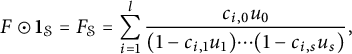 $$ \begin{align} F \odot \mathbf 1_{\mathcal{S}} = F_{\mathcal{S}} = \sum_{i=1}^l \frac{c_{i,0}u_0}{(1-c_{i,1}u_1)\cdots (1-c_{i,s}u_s)}, \end{align} $$
with $c_{i,\nu } \in K^*$
, with algebraically independent monomials
$c_{i,\nu } \in K^*$
, with algebraically independent monomials $u_1,\ldots ,u_s$
, and with an arbitrary monomial
$u_1,\ldots ,u_s$
, and with an arbitrary monomial $u_0$
. We first show that the coefficients in the denominators can be taken in G. After that, we will deal with the numerators and show that we can also achieve
$u_0$
. We first show that the coefficients in the denominators can be taken in G. After that, we will deal with the numerators and show that we can also achieve $l \le r$
.
$l \le r$
.
First, by combining summands with the same denominator, we may assume that no denominator occurs twice in (6.1). Then the uniqueness statement of Corollary 3.8, applied over the polynomial ring $K[u_1,\ldots ,u_s]$
, implies that the representation of
$K[u_1,\ldots ,u_s]$
, implies that the representation of $F_{\mathcal {S}}$
in this form is unique. In particular, each
$F_{\mathcal {S}}$
in this form is unique. In particular, each $1-c_{i,\nu }u_\nu $
indeed occurs as a factor of the reduced denominator of
$1-c_{i,\nu }u_\nu $
indeed occurs as a factor of the reduced denominator of $F_{\mathcal {S}}$
, considered as a rational function in
$F_{\mathcal {S}}$
, considered as a rational function in $K(u_1,\ldots ,u_s)$
.
$K(u_1,\ldots ,u_s)$
.
To deal with the denominators, it suffices to show that for every $i \in [1,l]$
and
$i \in [1,l]$
and $\nu \in [1,s]$
, there exists
$\nu \in [1,s]$
, there exists $N \ge 1$
such that
$N \ge 1$
such that $c_{i,\nu }^N \in G$
. Then we can use the remarks preceding this proposition to replace the denominators in such a way that the coefficients are in G. By symmetry, it suffices to show this for
$c_{i,\nu }^N \in G$
. Then we can use the remarks preceding this proposition to replace the denominators in such a way that the coefficients are in G. By symmetry, it suffices to show this for $i=\nu =1$
. Multiplying
$i=\nu =1$
. Multiplying $u_0^{-1}F_{\mathcal {S}}$
by a suitable polynomial in
$u_0^{-1}F_{\mathcal {S}}$
by a suitable polynomial in $K[u_1,\ldots ,u_s]$
to clear all denominators other than
$K[u_1,\ldots ,u_s]$
to clear all denominators other than $1-c_{1,1}u_1$
and setting
$1-c_{1,1}u_1$
and setting
, we obtain a rational series
with $1-cu_1$
not dividing
$1-cu_1$
not dividing $P(u_1,\ldots ,u_s) \in K[u_1,\ldots ,u_s]$
(note that the elements
$P(u_1,\ldots ,u_s) \in K[u_1,\ldots ,u_s]$
(note that the elements $1-c_{i,\nu }u_\nu $
are irreducible in
$1-c_{i,\nu }u_\nu $
are irreducible in $K[u_1,\ldots ,u_s]$
). By Lemma 2.6, there is a finite set B such that all coefficients of H are contained in
$K[u_1,\ldots ,u_s]$
). By Lemma 2.6, there is a finite set B such that all coefficients of H are contained in $BG_0$
.
$BG_0$
.
Working now in the polynomial ring $K[u_2,\ldots ,u_s][u_1]$
, we can use polynomial division to write
$K[u_2,\ldots ,u_s][u_1]$
, we can use polynomial division to write
 $$\begin{align*}P=Q(1-cu_1) + R \end{align*}$$
with $Q \in K[u_1,u_2,\ldots ,u_s]$
and
$Q \in K[u_1,u_2,\ldots ,u_s]$
and $0 \ne R \in K[u_2,\ldots ,u_s]$
. Fix any monomial
$0 \ne R \in K[u_2,\ldots ,u_s]$
. Fix any monomial $v \in \operatorname {\mathrm {supp}}(R)$
, and let its coefficient in R be a. Then, for large n,
$v \in \operatorname {\mathrm {supp}}(R)$
, and let its coefficient in R be a. Then, for large n,
 $$\begin{align*}[vu_1^n]H = a c^n \in BG_0. \end{align*}$$
For $b \in B$
, let
$b \in B$
, let $g_b \colon \mathbb {N} \to G_0$
be such that
$g_b \colon \mathbb {N} \to G_0$
be such that
 $$\begin{align*}a c^n = \sum_{b \in B} b g_b(n) \qquad\text{for large}\ n. \end{align*}$$
Fix a subset $B' \subseteq B$
such that, for infinitely many n,
$B' \subseteq B$
such that, for infinitely many n,
 $$\begin{align*}a c^n - \sum_{b \in B'} b g_b(n) = 0 \end{align*}$$
yields a nondegenerate solution to the unit equation $X_0 + \sum _{b \in B'} X_b=0$
over the group
$X_0 + \sum _{b \in B'} X_b=0$
over the group $G'$
generated by G,
$G'$
generated by G, $B'$
, and
$B'$
, and $-1$
. Let
$-1$
. Let $b \in B'$
. Then there exists a constant
$b \in B'$
. Then there exists a constant $\beta \in K^*$
such that
$\beta \in K^*$
such that
 $$\begin{align*}\frac{a c^{n}}{b g_b(n)} = \beta, \end{align*}$$
for infinitely many n. Let $n_1 < n_2$
be two such values. Then
$n_1 < n_2$
be two such values. Then
 $$\begin{align*}\frac{a c^{n_1}}{b g_b(n_1)} = \frac{a c^{n_2}}{b g_b(n_2)} \end{align*}$$
implies $c^{n_2-n_1} \in G$
. This finishes the claim about the denominators.
$c^{n_2-n_1} \in G$
. This finishes the claim about the denominators.
Going back to the representation of $F_{\mathcal {S}}$
in (6.1), and refining the set
$F_{\mathcal {S}}$
in (6.1), and refining the set $\mathcal {S}$
if necessary, we can therefore assume
$\mathcal {S}$
if necessary, we can therefore assume $c_{i,\nu } \in G$
for all
$c_{i,\nu } \in G$
for all $i \in [1,l]$
and
$i \in [1,l]$
and $\nu \in [1,s]$
. Using the same type of reduction, we may assume that whenever i,
$\nu \in [1,s]$
. Using the same type of reduction, we may assume that whenever i, $j \in [1,l]$
and
$j \in [1,l]$
and $\nu \in [1,s]$
are such that
$\nu \in [1,s]$
are such that $c_{i,\nu } \ne c_{j,\nu }$
, then
$c_{i,\nu } \ne c_{j,\nu }$
, then $c_{i,\nu }/c_{j,\nu }$
is not a root of unity.
$c_{i,\nu }/c_{j,\nu }$
is not a root of unity.
Now, we deal with the numerators $c_{0,\nu }$
for
$c_{0,\nu }$
for $\nu \in [1,s]$
and simultaneously with the number of summands. Let
$\nu \in [1,s]$
and simultaneously with the number of summands. Let $\boldsymbol c_i = (c_{i,1},\ldots ,c_{i,s})$
for
$\boldsymbol c_i = (c_{i,1},\ldots ,c_{i,s})$
for $i \in [1,l]$
, and
$i \in [1,l]$
, and $\boldsymbol u = (u_1,\ldots ,u_s)$
. Then
$\boldsymbol u = (u_1,\ldots ,u_s)$
. Then
 $$\begin{align*}[u_0\boldsymbol u^{\boldsymbol n}] F = \sum_{i=1}^l c_{i,0} \boldsymbol c_i^{\boldsymbol n} = g_1(\boldsymbol n) + \cdots + g_r(\boldsymbol n), \end{align*}$$
for some functions $g_1$
,
$g_1$
, $\ldots \,$
,
$\ldots \,$
, $g_r \colon \mathbb {N}^d \to G_0$
. Consider this as a unit equation over the group generated by G,
$g_r \colon \mathbb {N}^d \to G_0$
. Consider this as a unit equation over the group generated by G, $-1$
, and
$-1$
, and $c_{i,\nu }$
with
$c_{i,\nu }$
with $i \in [1,l]$
and
$i \in [1,l]$
and $\nu \in [0,s]$
.
$\nu \in [0,s]$
.
Consider a partition $\mathcal {P}=\{ (I_1,J_1), \ldots , (I_t,J_t) \}$
of the disjoint union
$\mathcal {P}=\{ (I_1,J_1), \ldots , (I_t,J_t) \}$
of the disjoint union $[1,l] \uplus [1,r]$
, that is,
$[1,l] \uplus [1,r]$
, that is, $I_\tau \subseteq [1,l]$
,
$I_\tau \subseteq [1,l]$
, $J_\tau \subseteq [1,r]$
, at least one of
$J_\tau \subseteq [1,r]$
, at least one of $I_\tau $
and
$I_\tau $
and $J_\tau $
is nonempty, and
$J_\tau $
is nonempty, and $I_\tau \cap I_{\tau '} = \emptyset = J_\tau \cap J_{\tau '}$
for
$I_\tau \cap I_{\tau '} = \emptyset = J_\tau \cap J_{\tau '}$
for $\tau \ne \tau '$
. Let
$\tau \ne \tau '$
. Let $\Omega _{\mathcal {P}} \subseteq \mathbb {N}^s$
denote the set of all
$\Omega _{\mathcal {P}} \subseteq \mathbb {N}^s$
denote the set of all $\boldsymbol n \in \mathbb {N}^s$
such that
$\boldsymbol n \in \mathbb {N}^s$
such that
 $$\begin{align*}\sum_{i \in I_\tau} c_{i,0} \boldsymbol c_i^{\boldsymbol n} - \sum_{j \in J_\tau} g_j(\boldsymbol n) =0 \end{align*}$$
yields a nondegenerate solution to the unit equation $\sum _{i \in I_{\tau }} X_i + \sum _{j \in J_\tau } X_j = 0$
. Then the sets
$\sum _{i \in I_{\tau }} X_i + \sum _{j \in J_\tau } X_j = 0$
. Then the sets $\Omega _{\mathcal {P}}$
cover
$\Omega _{\mathcal {P}}$
cover $\mathbb {N}^s$
as
$\mathbb {N}^s$
as $\mathcal {P}$
ranges through all partitions.
$\mathcal {P}$
ranges through all partitions.
We claim that there exists a partition $\mathcal {P}$
such that for all
$\mathcal {P}$
such that for all $i \ne j \in [1,l]$
the quotient
$i \ne j \in [1,l]$
the quotient $(\boldsymbol c_{i}/\boldsymbol c_j)^{\boldsymbol n}$
takes infinitely many values as
$(\boldsymbol c_{i}/\boldsymbol c_j)^{\boldsymbol n}$
takes infinitely many values as $\boldsymbol n$
ranges through
$\boldsymbol n$
ranges through $\Omega _{\mathcal {P}}$
. Suppose
$\Omega _{\mathcal {P}}$
. Suppose $\beta \in K^*$
. The set of all
$\beta \in K^*$
. The set of all $\boldsymbol n \in \mathbb {N}^s$
such that
$\boldsymbol n \in \mathbb {N}^s$
such that $(\boldsymbol c_i/\boldsymbol c_j)^{\boldsymbol n} = \beta $
is a semilinear set of rank at most
$(\boldsymbol c_i/\boldsymbol c_j)^{\boldsymbol n} = \beta $
is a semilinear set of rank at most $s-1$
by Lemma 6.3. Hence, if
$s-1$
by Lemma 6.3. Hence, if $(\boldsymbol c_i/\boldsymbol c_j)^{\boldsymbol n}$
takes finitely many values on
$(\boldsymbol c_i/\boldsymbol c_j)^{\boldsymbol n}$
takes finitely many values on $\Omega _{\mathcal {P}}$
, then
$\Omega _{\mathcal {P}}$
, then $\Omega _{\mathcal {P}}$
is contained in a semilinear set of rank at most
$\Omega _{\mathcal {P}}$
is contained in a semilinear set of rank at most $s-1$
. However, since the
$s-1$
. However, since the $\Omega _{\mathcal {P}}$
cover
$\Omega _{\mathcal {P}}$
cover $\mathbb {N}^s$
, there must be at least one
$\mathbb {N}^s$
, there must be at least one $\mathcal {P}$
such that
$\mathcal {P}$
such that $(\boldsymbol c_i/\boldsymbol c_j)^{\boldsymbol n}$
takes infinitely many values for
$(\boldsymbol c_i/\boldsymbol c_j)^{\boldsymbol n}$
takes infinitely many values for $\boldsymbol n \in \Omega _{\mathcal {P}}$
.
$\boldsymbol n \in \Omega _{\mathcal {P}}$
.
Now, fix such a partition $\mathcal {P}$
. Then necessarily
$\mathcal {P}$
. Then necessarily $ \left \lvert {I_\tau } \right \rvert \le 1$
for all
$ \left \lvert {I_\tau } \right \rvert \le 1$
for all $\tau \in [1,t]$
by the theorem on unit equations. If
$\tau \in [1,t]$
by the theorem on unit equations. If $I_\tau = \{i\}$
, it follows that
$I_\tau = \{i\}$
, it follows that
 $$\begin{align*}c_{i,0} = \sum_{j \in J_\tau} g_j(\boldsymbol n)/\boldsymbol c_i^{\boldsymbol n} \qquad\text{for}\ \boldsymbol n \in \Omega_{\mathcal{P}}. \end{align*}$$
Thus, $c_{i,0}$
is a sum of at most
$c_{i,0}$
is a sum of at most $ \left \lvert {J_\tau } \right \rvert $
elements of G. Substituting into (6.1) and splitting the sums accordingly (now we allow the same denominator to appear multiple times), we achieve
$ \left \lvert {J_\tau } \right \rvert $
elements of G. Substituting into (6.1) and splitting the sums accordingly (now we allow the same denominator to appear multiple times), we achieve $c_{i,0} \in G$
and
$c_{i,0} \in G$
and $l \le \left \lvert {J_1} \right \rvert + \cdots + \left \lvert {J_t} \right \rvert \le r$
in this representation.
$l \le \left \lvert {J_1} \right \rvert + \cdots + \left \lvert {J_t} \right \rvert \le r$
in this representation.
7 Proofs of main theorems
At this point, Theorems 1.2 and 1.3 can easily be proved as follows.
Proof of Theorem 1.2
(a) $\,\Rightarrow \,$
(b) By Theorem 4.1, every D-finite Bézivin series is rational.
$\,\Rightarrow \,$
(b) By Theorem 4.1, every D-finite Bézivin series is rational.
(b) $\,\Rightarrow \,$
(d) Let
$\,\Rightarrow \,$
(d) Let
![]() be a rational Bézivin series. By Proposition 6.1, the series is a trivially ambiguous sum of skew-geometric series. That the constants in the skew-geometric summands can be taken in G, and that the sum can be taken in such a way that no
be a rational Bézivin series. By Proposition 6.1, the series is a trivially ambiguous sum of skew-geometric series. That the constants in the skew-geometric summands can be taken in G, and that the sum can be taken in such a way that no $\boldsymbol n \in \mathbb {N}^d$
is contained in the support of more than r summands, follows from Proposition 6.4.
$\boldsymbol n \in \mathbb {N}^d$
is contained in the support of more than r summands, follows from Proposition 6.4.
(d) $\,\Rightarrow \,$
(c) Clear.
$\,\Rightarrow \,$
(c) Clear.
(c) $\,\Rightarrow \,$
(a) Trivial, because every rational series is D-finite.
$\,\Rightarrow \,$
(a) Trivial, because every rational series is D-finite.
(d) $\,\Leftrightarrow \,$
(e) This equivalence is immediate from the definition of a skew-geometric series, Definition 3.15, together with Lemma 3.4.
$\,\Leftrightarrow \,$
(e) This equivalence is immediate from the definition of a skew-geometric series, Definition 3.15, together with Lemma 3.4.
Proof of Theorem 1.3
We apply Theorem 1.2 with $r=1$
. Then (a)
$r=1$
. Then (a) $\,\Leftrightarrow \,$
(b) of Theorem 1.3 follows from (a)
$\,\Leftrightarrow \,$
(b) of Theorem 1.3 follows from (a) $\,\Leftrightarrow \,$
(b) of Theorem 1.2. The implication (b)
$\,\Leftrightarrow \,$
(b) of Theorem 1.2. The implication (b) $\,\Rightarrow \,$
(c) of Theorem 1.3 follows from (b)
$\,\Rightarrow \,$
(c) of Theorem 1.3 follows from (b) $\,\Rightarrow \,$
(d) of Theorem 1.2, taking into account
$\,\Rightarrow \,$
(d) of Theorem 1.2, taking into account $r=1$
.
$r=1$
.
To obtain (c) $\,\Rightarrow \,$
(d) of Theorem 1.3, apply (d)
$\,\Rightarrow \,$
(d) of Theorem 1.3, apply (d) $\,\Rightarrow \,$
(e) of Theorem 1.2, noting again
$\,\Rightarrow \,$
(e) of Theorem 1.2, noting again $r=1$
. This gives a partition of
$r=1$
. This gives a partition of $\mathbb {N}^d$
into simple linear sets, so that on each such set
$\mathbb {N}^d$
into simple linear sets, so that on each such set $\mathcal {S} = \boldsymbol a_0 + \boldsymbol a_1 \mathbb {N} + \cdots + \boldsymbol a_s \mathbb {N}$
, one has
$\mathcal {S} = \boldsymbol a_0 + \boldsymbol a_1 \mathbb {N} + \cdots + \boldsymbol a_s \mathbb {N}$
, one has $f(\boldsymbol a_0 + m_1 \boldsymbol a_1 + \cdots + m_s \boldsymbol a_s) = 0$
or
$f(\boldsymbol a_0 + m_1 \boldsymbol a_1 + \cdots + m_s \boldsymbol a_s) = 0$
or $f(\boldsymbol a_0 + m_1 \boldsymbol a_1 + \cdots + m_s \boldsymbol a_s) = g_0 g_1^{m_1} \cdots g_s^{m_s} \ne 0$
with
$f(\boldsymbol a_0 + m_1 \boldsymbol a_1 + \cdots + m_s \boldsymbol a_s) = g_0 g_1^{m_1} \cdots g_s^{m_s} \ne 0$
with $g_0$
,
$g_0$
, $g_1$
,
$g_1$
, $\ldots \,$
,
$\ldots \,$
, $g_s \in G$
. Taking only these simple linear sets of the partition on which f does not vanish, we obtain a partition of the support of F, as claimed.
$g_s \in G$
. Taking only these simple linear sets of the partition on which f does not vanish, we obtain a partition of the support of F, as claimed.
Finally, the implication (d) $\,\Rightarrow \,$
(a) of Theorem 1.3 follows from the implication (e)
$\,\Rightarrow \,$
(a) of Theorem 1.3 follows from the implication (e) $\,\Rightarrow \,$
(a) of Theorem 1.2.
$\,\Rightarrow \,$
(a) of Theorem 1.2.
Before proving Corollary 1.4, we show that algebraic series and their diagonals and sections are finitary D-finite. Recall that the operator
![]() assigns to
assigns to
 $$\begin{align*}F=\sum_{n_1,n_2,\ldots,n_d \in \mathbb{N}} f(n_1,n_2,n_3,\ldots,n_d) x_1^{n_1}x_2^{n_2}x_3^{n_3}\cdots x_d^{n_d} \end{align*}$$
its primitive diagonal
 $$\begin{align*}I_{1,2}F = \sum_{n_1,n_3,\ldots n_d \in \mathbb{N}} f(n_1,n_1,n_3,\ldots,n_d) x_1^{n_1} x_3^{n_3} \cdots x_d^{n_d}. \end{align*}$$
For $1 \le i < j \le d$
, the primitive diagonal operators
$1 \le i < j \le d$
, the primitive diagonal operators $I_{i,j}$
are defined analogously. A diagonal of F is any composition of diagonal operators applied to F. For instance, the complete diagonal of F is
$I_{i,j}$
are defined analogously. A diagonal of F is any composition of diagonal operators applied to F. For instance, the complete diagonal of F is $I_{1,2}I_{2,3}\cdots I_{d-1,d}F = \sum _{n \in \mathbb {N}} f(n,n,\ldots ,n) x_1^n$
. A series
$I_{1,2}I_{2,3}\cdots I_{d-1,d}F = \sum _{n \in \mathbb {N}} f(n,n,\ldots ,n) x_1^n$
. A series
![]() is algebraic if it is algebraic over the field
is algebraic if it is algebraic over the field $K(\boldsymbol x)$
.
$K(\boldsymbol x)$
.
Lemma 7.1 If
![]() is:
is:
-
• algebraic, or
-
• a diagonal of an algebraic series, or
-
• a section of an algebraic series,
then F is finitary D-finite.
Proof Algebraic series are D-finite, and diagonals and sections of D-finite series are D-finite [Reference LipshitzLip89, Proposition 2.5 and Theorem 2.7]. Moreover, diagonals and sections of finitary series are trivially finitary. It therefore suffices to show that algebraic series are finitary.
Let
![]() be algebraic. Replacing F by
be algebraic. Replacing F by $F - F(0)$
, we may assume
$F - F(0)$
, we may assume $F(0)=0$
. Since F is algebraic, there exist
$F(0)=0$
. Since F is algebraic, there exist $p_2$
,
$p_2$
, $\ldots \,$
,
$\ldots \,$
, $p_m$
,
$p_m$
, $q \in K[{\boldsymbol x}]$
with
$q \in K[{\boldsymbol x}]$
with $q \ne 0$
such that
$q \ne 0$
such that $F = \frac {p_2}{q} F^2 + \cdots + \frac {p_m}{q} F^m$
. Setting
$F = \frac {p_2}{q} F^2 + \cdots + \frac {p_m}{q} F^m$
. Setting $G = F/q$
and multiplying the previous equation by
$G = F/q$
and multiplying the previous equation by $1/q$
, we obtain an equation
$1/q$
, we obtain an equation
 $$\begin{align*}G = p_2 G^2 + p_3q G^3 + \cdots + p_m q^{m-2} G^m. \end{align*}$$
Keeping in mind $G(0)=0$
, this yields a recursion for the coefficients of G. It follows from this recursion that G is finitary. Since
$G(0)=0$
, this yields a recursion for the coefficients of G. It follows from this recursion that G is finitary. Since $F=qG$
, also F is finitary.
$F=qG$
, also F is finitary.
Lemma 7.2 If
![]() is a finitary series and
is a finitary series and $F^\dagger $
is also finitary, then F is a Pólya series.
$F^\dagger $
is also finitary, then F is a Pólya series.
Proof Since F is finitary, there is a finitely generated $\mathbb {Z}$
-algebra
$\mathbb {Z}$
-algebra $A \subseteq K$
containing all coefficients of K. Since
$A \subseteq K$
containing all coefficients of K. Since $F^\dagger $
is finitary as well, we may also assume that A contains
$F^\dagger $
is finitary as well, we may also assume that A contains $f(\boldsymbol n)^{-1}$
whenever
$f(\boldsymbol n)^{-1}$
whenever $f(\boldsymbol n) \ne 0$
. Therefore, all nonzero coefficients of F are contained in the unit group G of A. By a theorem of Roquette (see [Reference LangLan83, Corollary 7.5 of Chapter 2]), the group G is finitely generated.
$f(\boldsymbol n) \ne 0$
. Therefore, all nonzero coefficients of F are contained in the unit group G of A. By a theorem of Roquette (see [Reference LangLan83, Corollary 7.5 of Chapter 2]), the group G is finitely generated.
Proof of Corollary 1.4
Since F and $F^\dagger $
are finitary, F is a Pólya series by Lemma 7.2. Being also D-finite, F satisfies condition (a) of Theorem 1.3. Conversely, if F satisfies condition (d) of Theorem 1.3, then clearly the same is true for
$F^\dagger $
are finitary, F is a Pólya series by Lemma 7.2. Being also D-finite, F satisfies condition (a) of Theorem 1.3. Conversely, if F satisfies condition (d) of Theorem 1.3, then clearly the same is true for $F^\dagger $
. Thus, the series
$F^\dagger $
. Thus, the series $F^\dagger $
is D-finite.
$F^\dagger $
is D-finite.
The “in particular” statement of the corollary follows from Theorem 1.3 applied to F, respectively, $F^\dagger $
.
$F^\dagger $
.


 Open access