


1. Introduction
Ramsey theory is one of the most studied areas in modern combinatorics. Let $r \in \mathbb{N}$
and let
$r \in \mathbb{N}$
and let $G, H_1, \ldots, H_r$
be graphs. We write
$G, H_1, \ldots, H_r$
be graphs. We write $G \to (H_1, \ldots, H_r)$
to denote the property that whenever we colour the edges of
$G \to (H_1, \ldots, H_r)$
to denote the property that whenever we colour the edges of $G$
with colours from the set
$G$
with colours from the set $[r] \,{:\!=}\, \{1, \ldots, r\}$
there exists
$[r] \,{:\!=}\, \{1, \ldots, r\}$
there exists $i \in [r]$
and a copy of
$i \in [r]$
and a copy of $H_i$
in
$H_i$
in $G$
monochromatic in colour
$G$
monochromatic in colour $i$
. Thus, in this notation, the classical result of Ramsey [Reference Ramsey18] asserts that for
$i$
. Thus, in this notation, the classical result of Ramsey [Reference Ramsey18] asserts that for $n$
sufficiently large
$n$
sufficiently large $K_n \to (H_1, \ldots, H_r)$
. One may posit that this is only true because
$K_n \to (H_1, \ldots, H_r)$
. One may posit that this is only true because $K_n$
is very dense, but Folkman [Reference Folkman2], and in a more general setting Nešetřil and Rödl [Reference Nešetřil and Rödl17], proved that for any graph
$K_n$
is very dense, but Folkman [Reference Folkman2], and in a more general setting Nešetřil and Rödl [Reference Nešetřil and Rödl17], proved that for any graph $H$
there are locally sparse graphs
$H$
there are locally sparse graphs $G = G(H)$
such that
$G = G(H)$
such that $G \to (H_1, \ldots, H_r)$
when
$G \to (H_1, \ldots, H_r)$
when $H_1 = \cdots = H_r = H$
.
$H_1 = \cdots = H_r = H$
.
1.1 Symmetric Ramsey properties: Rödl and Ruciński’s theorem
If we transfer our study of the Ramsey property to the random setting, we discover that such graphs $G$
are in fact very common. Let
$G$
are in fact very common. Let $G_{n,p}$
be the binomial random graph with
$G_{n,p}$
be the binomial random graph with $n$
vertices and edge probability
$n$
vertices and edge probability $p$
. Improving on earlier work of Frankl and Rödl [Reference Frankl and Rödl3], Łuczak, Ruciński and Voigt [Reference Łuczak, Ruciński and Voigt13] proved that
$p$
. Improving on earlier work of Frankl and Rödl [Reference Frankl and Rödl3], Łuczak, Ruciński and Voigt [Reference Łuczak, Ruciński and Voigt13] proved that $p = n^{-1/2}$
is a threshold for the property
$p = n^{-1/2}$
is a threshold for the property $G_{n,p} \to (K_3, K_3)$
. Following this, Rödl and Ruciński [Reference Rödl and Ruciński19–Reference Rödl and Ruciński21] determined a threshold for the general symmetric case. For a graph
$G_{n,p} \to (K_3, K_3)$
. Following this, Rödl and Ruciński [Reference Rödl and Ruciński19–Reference Rödl and Ruciński21] determined a threshold for the general symmetric case. For a graph $H$
, we define
$H$
, we define
 \begin{align*} d_2(H) \,{:\!=}\, \begin{cases} (e_H - 1)/(v_H - 2) & \quad \text{if } H \text{ is non-empty with} \ v(H) \geq 3,\\ \\[-8pt] 1/2 & \quad \text{if} \ H \cong K_2,\\ \\[-8pt] 0 & \quad \text{otherwise} \end{cases} \end{align*}
and the $2$
-density of
$2$
-density of $H$
to be
$H$
to be
 \begin{equation*} m_2(H) \,{:\!=}\, \max \{d_2(J)\,{:}\, J \subseteq H\}. \end{equation*}
We say that a graph $H$
is
$H$
is $2$
-balanced if
$2$
-balanced if $d_2(H) = m_2(H)$
, and strictly 2-balanced if for all proper subgraphs
$d_2(H) = m_2(H)$
, and strictly 2-balanced if for all proper subgraphs $J \subsetneq H$
, we have
$J \subsetneq H$
, we have $d_2(J) \lt m_2(H)$
.
$d_2(J) \lt m_2(H)$
.
Theorem 1.1. (Rödl and Ruciński [Reference Rödl and Ruciński21]) Let $r \geq 2$
and let
$r \geq 2$
and let $H$
be a non-empty graph such that at least one component of
$H$
be a non-empty graph such that at least one component of $H$
is not a star. If
$H$
is not a star. If $r = 2$
, then in addition restrict
$r = 2$
, then in addition restrict $H$
to having no component which is a path on
$H$
to having no component which is a path on $3$
edges. Then there exist positive constants
$3$
edges. Then there exist positive constants $b, B \gt 0$
such that
$b, B \gt 0$
such that
 \begin{align*} \lim \limits _{n \to \infty } \mathbb{P}[G_{n,p} \to (\underbrace{\!H, \ldots, H\!}_{r \ times})] = \begin{cases} 0 & \quad \text{if } p \leq bn^{-1/m_2(H)},\\ \\[-8pt] 1 & \quad \text{if } p \geq Bn^{-1/m_2(H)}. \end{cases} \end{align*}
The statement for $p \leq bn^{-1/m_2(H)}$
in Theorem 1.1 is known as a
$p \leq bn^{-1/m_2(H)}$
in Theorem 1.1 is known as a $0$
-statement and the statement for
$0$
-statement and the statement for $p \geq Bn^{-1/m_2(H)}$
is known as a
$p \geq Bn^{-1/m_2(H)}$
is known as a $1$
-statement.
$1$
-statement.
The assumption on the structure of $H$
in Theorem 1.1 is necessary. If every component of
$H$
in Theorem 1.1 is necessary. If every component of $H$
is a star then
$H$
is a star then $G_{n,p} \to (H, \ldots, H)$
as soon as sufficiently many vertices of degree
$G_{n,p} \to (H, \ldots, H)$
as soon as sufficiently many vertices of degree $r(\Delta (H) - 1) + 1$
appear in
$r(\Delta (H) - 1) + 1$
appear in $G_{n,p}$
. A threshold for this property in
$G_{n,p}$
. A threshold for this property in $G_{n,p}$
is
$G_{n,p}$
is $p = n^{-1-1/(r(\Delta (H) - 1) + 1)}$
, but
$p = n^{-1-1/(r(\Delta (H) - 1) + 1)}$
, but $m_2(H) = 1$
. For the case when
$m_2(H) = 1$
. For the case when $r = 2$
and at least one component of
$r = 2$
and at least one component of $H$
is a path on 3 edges while the others are stars, the
$H$
is a path on 3 edges while the others are stars, the $0$
-statement of Theorem 1.1 becomes false. Indeed, one can show that, if
$0$
-statement of Theorem 1.1 becomes false. Indeed, one can show that, if $p = cn^{-1/m_2(P_3)} = cn^{-1}$
for some
$p = cn^{-1/m_2(P_3)} = cn^{-1}$
for some $c \gt 0$
, then the probability that
$c \gt 0$
, then the probability that $G_{n,p}$
contains a cycle of length 5 with an edge pending at every vertex is bounded from below by a positive constant
$G_{n,p}$
contains a cycle of length 5 with an edge pending at every vertex is bounded from below by a positive constant $d = d(c)$
. One can check that every colouring of the edges of this augmented
$d = d(c)$
. One can check that every colouring of the edges of this augmented $5$
-cycle with 2 colours yields a monochromatic path of length 3. This special case was missed in [Reference Rödl and Ruciński21], and was eventually observed by Friedgut and Krivelevich [Reference Friedgut and Krivelevich4], who corrected the
$5$
-cycle with 2 colours yields a monochromatic path of length 3. This special case was missed in [Reference Rödl and Ruciński21], and was eventually observed by Friedgut and Krivelevich [Reference Friedgut and Krivelevich4], who corrected the $0$
-statement to have the assumption
$0$
-statement to have the assumption $p = o(n^{-1/m_2(H)})$
instead. Note that Nenadov and Steger [Reference Nenadov and Steger16] produced a short proof of Theorem 1.1 using the hypergraph container method.
$p = o(n^{-1/m_2(H)})$
instead. Note that Nenadov and Steger [Reference Nenadov and Steger16] produced a short proof of Theorem 1.1 using the hypergraph container method.
The intuition behind the threshold in Theorem 1.1 is as follows: Firstly, assume $H$
is
$H$
is $2$
-balanced. The expected number of copies of a graph
$2$
-balanced. The expected number of copies of a graph $H$
in
$H$
in $G_{n,p}$
is
$G_{n,p}$
is $\Theta (n^{v(H)}p^{e(H)})$
and the expected number of edges is
$\Theta (n^{v(H)}p^{e(H)})$
and the expected number of edges is $\Theta (n^2p)$
. For
$\Theta (n^2p)$
. For $p = n^{-1/m_2(H)}$
(the threshold in Theorem 1.1), these two expectations are of the same order since
$p = n^{-1/m_2(H)}$
(the threshold in Theorem 1.1), these two expectations are of the same order since $H$
is
$H$
is $2$
-balanced. That is to say, if the expected number of copies of
$2$
-balanced. That is to say, if the expected number of copies of $H$
at a fixed edge is smaller than some small constant
$H$
at a fixed edge is smaller than some small constant $c$
, then we can hope to colour without creating a monochromatic copy of
$c$
, then we can hope to colour without creating a monochromatic copy of $H$
: very roughly speaking, each copy will likely contain an edge not belonging to any other copy of
$H$
: very roughly speaking, each copy will likely contain an edge not belonging to any other copy of $H$
, so by colouring these edges with one colour and all other edges with a different colour we avoid creating monochromatic copies of
$H$
, so by colouring these edges with one colour and all other edges with a different colour we avoid creating monochromatic copies of $H$
. If the expected number of copies of
$H$
. If the expected number of copies of $H$
at a fixed edge is larger than some large constant
$H$
at a fixed edge is larger than some large constant $C$
then a monochromatic copy of
$C$
then a monochromatic copy of $H$
may appear in any
$H$
may appear in any $r$
-colouring since the copies of
$r$
-colouring since the copies of $H$
most likely overlap heavily.
$H$
most likely overlap heavily.
Sharp thresholds for $G_{n,p} \to (H,H)$
have also been obtained when
$G_{n,p} \to (H,H)$
have also been obtained when $H$
is a tree [Reference Friedgut and Krivelevich4], a triangle [Reference Friedgut, Rödl, Ruciński and Tetali5] or, more generally, a strictly
$H$
is a tree [Reference Friedgut and Krivelevich4], a triangle [Reference Friedgut, Rödl, Ruciński and Tetali5] or, more generally, a strictly $2$
-balanced graph that can be made bipartite by the removal of some edge [Reference Schacht and Schulenburg22].
$2$
-balanced graph that can be made bipartite by the removal of some edge [Reference Schacht and Schulenburg22].
Theorem 1.2. ([Reference Friedgut and Krivelevich4, Reference Friedgut, Rödl, Ruciński and Tetali5, Reference Schacht and Schulenburg22]) Suppose that $H$
is either (i) a tree that is not a star or the path of length three or (ii) a strictly
$H$
is either (i) a tree that is not a star or the path of length three or (ii) a strictly $2$
-balanced graph with
$2$
-balanced graph with $e(H) \geq 2$
that can be made bipartite by the removal of some edge. Then there exist constants
$e(H) \geq 2$
that can be made bipartite by the removal of some edge. Then there exist constants $c_0$
,
$c_0$
, $c_1$
, and a function
$c_1$
, and a function $c\,{:}\, \mathbb{N} \to [c_0, c_1]$
, such that
$c\,{:}\, \mathbb{N} \to [c_0, c_1]$
, such that
 \begin{align*} \lim \limits _{n \to \infty } \mathbb{P}[G_{n,p} \to (H, H)] = \begin{cases} 0 & \quad \textit{if}\ p \leq (1 - \varepsilon )c(n)n^{-1/m_2(H)},\\[3pt] 1 & \quad \textit{if}\ p \geq (1 + \varepsilon )c(n)n^{-1/m_2(H)}\end{cases} \end{align*}
for every positive constant $\varepsilon$
.
$\varepsilon$
.
1.2 Asymmetric Ramsey properties: The Kohayakawa-Kreuter Conjecture
In this paper, we are interested in asymmetric Ramsey properties of $G_{n,p}$
, that is, finding a threshold for when
$G_{n,p}$
, that is, finding a threshold for when $G_{n,p} \to (H_1 \ldots, H_r)$
and
$G_{n,p} \to (H_1 \ldots, H_r)$
and $H_1, \ldots, H_r$
are not all the same graph. In classical Ramsey theory, the study of asymmetric Ramsey properties sparked off many interesting routes of research (see, e.g. [Reference Chung and Graham1]), including the seminal work of Kim [Reference Kim9] on establishing an asymptotically sharp lower bound on the Ramsey number
$H_1, \ldots, H_r$
are not all the same graph. In classical Ramsey theory, the study of asymmetric Ramsey properties sparked off many interesting routes of research (see, e.g. [Reference Chung and Graham1]), including the seminal work of Kim [Reference Kim9] on establishing an asymptotically sharp lower bound on the Ramsey number $R(3,t)$
. In
$R(3,t)$
. In $G_{n,p}$
, asymmetric Ramsey properties were first considered by Kohayakawa and Kreuter [Reference Kohayakawa and Kreuter10]. For graphs
$G_{n,p}$
, asymmetric Ramsey properties were first considered by Kohayakawa and Kreuter [Reference Kohayakawa and Kreuter10]. For graphs $H_1$
and
$H_1$
and $H_2$
with
$H_2$
with $m_2(H_1) \geq m_2(H_2)$
, we define
$m_2(H_1) \geq m_2(H_2)$
, we define
 \begin{align*} d_2(H_1,H_2) \,{:\!=}\, \begin{cases} \dfrac{e(H_1)}{v(H_1) - 2 + \frac{1}{m_2(H_2)}} & \quad \text{if } H_2 \text{ is non-empty and} \ v(H_1) \geq 2,\\ \\[-8pt] 0 & \quad \text{otherwise} \end{cases} \end{align*}
and the asymmetric 2-density of the pair ( $H_1$
,
$H_1$
, $H_2$
) to be
$H_2$
) to be
 \begin{align*} m_2(H_1, H_2) \,{:\!=}\, \max \!\left \{d_2(J,H_2)\,{:}\, J \subseteq H_1\right \}. \end{align*}
We say that $H_1$
is balanced with respect to
$H_1$
is balanced with respect to $d_2(\cdot, H_2)$
if we have
$d_2(\cdot, H_2)$
if we have $d_2(H_1, H_2) = m_2(H_1, H_2)$
and strictly balanced with respect to
$d_2(H_1, H_2) = m_2(H_1, H_2)$
and strictly balanced with respect to $d_2(\cdot, H_2)$
if for all proper subgraphs
$d_2(\cdot, H_2)$
if for all proper subgraphs $J \subsetneq H_1$
we have
$J \subsetneq H_1$
we have $d_2(J, H_2) \lt m_2(H_1, H_2)$
. Note that
$d_2(J, H_2) \lt m_2(H_1, H_2)$
. Note that $m_2(H_1) \geq m_2(H_1, H_2) \geq m_2(H_2)$
(see Proposition 1.7).
$m_2(H_1) \geq m_2(H_1, H_2) \geq m_2(H_2)$
(see Proposition 1.7).
Kohayakawa and Kreuter [Reference Kohayakawa and Kreuter10] conjectured the following generalisation of Theorem 1.1. (We give here a slight rephrasing of the conjecture: we consider $r$
colours (instead of 2) and add the assumption of Kohayakawa, Schacht and Spöhel [Reference Kohayakawa, Schacht and Spöhel11] that
$r$
colours (instead of 2) and add the assumption of Kohayakawa, Schacht and Spöhel [Reference Kohayakawa, Schacht and Spöhel11] that $H_1$
and
$H_1$
and $H_2$
are not forests.Footnote 1)
$H_2$
are not forests.Footnote 1)
Conjecture 1.3. (Kohayakawa and Kreuter [Reference Kohayakawa and Kreuter10]) Let $r \geq 2$
and suppose that
$r \geq 2$
and suppose that $H_1, \ldots, H_r$
are non-empty graphs such that
$H_1, \ldots, H_r$
are non-empty graphs such that $m_2(H_1) \geq \cdots \geq m_2(H_r)$
and
$m_2(H_1) \geq \cdots \geq m_2(H_r)$
and $m_2(H_2) \gt 1$
. Then there exist constants
$m_2(H_2) \gt 1$
. Then there exist constants $b, B \gt 0$
such that
$b, B \gt 0$
such that
 \begin{align*} \lim \limits _{n \to \infty } \mathbb{P}[G_{n,p} \to (H_1, \ldots, H_r)] = \begin{cases} 0 & \quad \text{if } p \leq bn^{-1/m_2(H_1,H_2)},\\ \\[-8pt]1 & \quad \text{if } p \geq Bn^{-1/m_2(H_1,H_2)}. \end{cases} \end{align*}
Observe that we would always need $m_2(H_2) \geq 1$
as an assumption, otherwise
$m_2(H_2) \geq 1$
as an assumption, otherwise $m_2(H_2) = 1/2$
(that is,
$m_2(H_2) = 1/2$
(that is, $H_2$
is the union of a matching and some isolated vertices) and we would have that
$H_2$
is the union of a matching and some isolated vertices) and we would have that $m_2(H_1, H_2) = e_J/v_J$
for some non-empty subgraph
$m_2(H_1, H_2) = e_J/v_J$
for some non-empty subgraph $J \subseteq H_1$
. For any constant
$J \subseteq H_1$
. For any constant $B \gt 0$
, the probability that
$B \gt 0$
, the probability that $G_{n,p}$
with
$G_{n,p}$
with $p = Bn^{-1/m_2(H_1, H_2)}$
contains no copy of
$p = Bn^{-1/m_2(H_1, H_2)}$
contains no copy of $H_1$
exceeds a positive constant
$H_1$
exceeds a positive constant $C = C(B)$
; see, for example [Reference Janson, Łuczak and Ruciński8]. We include the assumption of Kohayakawa, Schacht and Spöhel [Reference Kohayakawa, Schacht and Spöhel11], that
$C = C(B)$
; see, for example [Reference Janson, Łuczak and Ruciński8]. We include the assumption of Kohayakawa, Schacht and Spöhel [Reference Kohayakawa, Schacht and Spöhel11], that $m_2(H_2) \gt 1$
, to avoid possible complications arising from
$m_2(H_2) \gt 1$
, to avoid possible complications arising from $H_2$
(and/or
$H_2$
(and/or $H_1$
) being certain forests, such as those excluded in the statement of Theorem 1.1.
$H_1$
) being certain forests, such as those excluded in the statement of Theorem 1.1.
The intuition behind the threshold in Conjecture 1.3 is most readily explained in the case of $r = 3$
,
$r = 3$
, $H_2 = H_3$
and when
$H_2 = H_3$
and when $m_2(H_1) \gt m_2(H_1, H_2)$
. (The following explanation is adapted from [Reference Gugelmann, Nenadov, Person, Škorić, Steger and Thomas6].) Firstly, observe that we can assign colour 1 to every edge that does not lie in a copy of
$m_2(H_1) \gt m_2(H_1, H_2)$
. (The following explanation is adapted from [Reference Gugelmann, Nenadov, Person, Škorić, Steger and Thomas6].) Firstly, observe that we can assign colour 1 to every edge that does not lie in a copy of $H_1$
. Since
$H_1$
. Since $m_2(H_1) \gt m_2(H_1, H_2)$
, we expect that the copies of
$m_2(H_1) \gt m_2(H_1, H_2)$
, we expect that the copies of $H_1$
in
$H_1$
in $G_{n,p}$
with
$G_{n,p}$
with $p = \Theta (n^{-1/m_2(H_1,H_2)})$
do not overlap much (by similar reasoning as in the intuition for the threshold in Theorem 1.1). Hence the number of edges left to be coloured is of the same order as the number of copies of
$p = \Theta (n^{-1/m_2(H_1,H_2)})$
do not overlap much (by similar reasoning as in the intuition for the threshold in Theorem 1.1). Hence the number of edges left to be coloured is of the same order as the number of copies of $H_1$
, which is
$H_1$
, which is $\Theta (n^{v(H_1)}p^{e(H_1)})$
. If we further assume that these edges are randomly distributed (which is not correct, but gives good intuition) then we get a random graph
$\Theta (n^{v(H_1)}p^{e(H_1)})$
. If we further assume that these edges are randomly distributed (which is not correct, but gives good intuition) then we get a random graph $G^*$
with edge probability
$G^*$
with edge probability $p^* = \Theta (n^{v(H_1) - 2}p^{e(H_1)})$
. Now we colour
$p^* = \Theta (n^{v(H_1) - 2}p^{e(H_1)})$
. Now we colour $G^*$
with colours 2 and 3, and apply the intuition from the symmetric case (as
$G^*$
with colours 2 and 3, and apply the intuition from the symmetric case (as $H_2 = H_3$
): if the copies of
$H_2 = H_3$
): if the copies of $H_2$
are heavily overlapping then we cannot hope to colour without getting a monochromatic copy of
$H_2$
are heavily overlapping then we cannot hope to colour without getting a monochromatic copy of $H_2$
, but if not then we should be able to colour. As observed before, a threshold for this property is
$H_2$
, but if not then we should be able to colour. As observed before, a threshold for this property is $p^* = n^{-1/m_2(H_2)}$
. Solving
$p^* = n^{-1/m_2(H_2)}$
. Solving $n^{v(H_1) - 2}p^{e(H_1)} = n^{-1/m_2(H_2)}$
for
$n^{v(H_1) - 2}p^{e(H_1)} = n^{-1/m_2(H_2)}$
for $p$
then yields
$p$
then yields $p = n^{-1/m_2(H_1,H_2)}$
, the conjectured threshold.
$p = n^{-1/m_2(H_1,H_2)}$
, the conjectured threshold.
After earlier work (see e.g. [Reference Gugelmann, Nenadov, Person, Škorić, Steger and Thomas6, Reference Hancock, Staden and Treglown7, Reference Kohayakawa and Kreuter10, Reference Kohayakawa, Schacht and Spöhel11, Reference Marciniszyn, Skokan, Spöhel and Steger14]), the $1$
-statement of Conjecture 1.3 was proven by Mousset, Nenadov and Samotij [Reference Mousset, Nenadov and Samotij15].
$1$
-statement of Conjecture 1.3 was proven by Mousset, Nenadov and Samotij [Reference Mousset, Nenadov and Samotij15].
1.3 The $0$
-statement of the Kohayakawa-Kreuter Conjecture
$0$
-statement of the Kohayakawa-Kreuter Conjecture

In this paper, we are interested in the $0$
-statement of Conjecture 1.3, which has so far only been proven when
$0$
-statement of Conjecture 1.3, which has so far only been proven when $H_1$
and
$H_1$
and $H_2$
are both cycles [Reference Kohayakawa and Kreuter10], both cliques [Reference Marciniszyn, Skokan, Spöhel and Steger14] and, recently, when
$H_2$
are both cycles [Reference Kohayakawa and Kreuter10], both cliques [Reference Marciniszyn, Skokan, Spöhel and Steger14] and, recently, when $H_1$
is a clique and
$H_1$
is a clique and $H_2$
is a cycle [Reference Liebenau, Mattos, Mendonça and Skokan12]. We also note that the authors of [Reference Gugelmann, Nenadov, Person, Škorić, Steger and Thomas6] prove, under certain balancedness conditions, the
$H_2$
is a cycle [Reference Liebenau, Mattos, Mendonça and Skokan12]. We also note that the authors of [Reference Gugelmann, Nenadov, Person, Škorić, Steger and Thomas6] prove, under certain balancedness conditions, the $0$
-statement of a generalised version of Conjecture 1.3 which allows
$0$
-statement of a generalised version of Conjecture 1.3 which allows $H_1, \ldots, H_r$
to be uniform hypergraphs.
$H_1, \ldots, H_r$
to be uniform hypergraphs.
Definition 1.4. Let $H_1$
and
$H_1$
and $H_2$
be non-empty graphs. We say that a graph
$H_2$
be non-empty graphs. We say that a graph $G$
has a valid edge-colouring for
$G$
has a valid edge-colouring for $H_1$
and
$H_1$
and $H_2$
if there exists a red/blue colouring of the edges of
$H_2$
if there exists a red/blue colouring of the edges of $G$
that does not produce a red copy of
$G$
that does not produce a red copy of $H_1$
or a blue copy of
$H_1$
or a blue copy of $H_2$
.
$H_2$
.
To prove the $0$
-statement of Conjecture 1.3, one only needs to show that
$0$
-statement of Conjecture 1.3, one only needs to show that $G = G_{n,p}$
has a valid edge-colouring for
$G = G_{n,p}$
has a valid edge-colouring for $H_1$
and
$H_1$
and $H_2$
asymptotically almost surely (a.a.s.) (that is, we ignore
$H_2$
asymptotically almost surely (a.a.s.) (that is, we ignore $H_3, \ldots, H_r$
and colours
$H_3, \ldots, H_r$
and colours $3, \ldots, r$
). Further, when
$3, \ldots, r$
). Further, when $m_2(H_1) \gt m_2(H_2)$
we can assume when trying to prove the
$m_2(H_1) \gt m_2(H_2)$
we can assume when trying to prove the $0$
-statement of Conjecture 1.3 that
$0$
-statement of Conjecture 1.3 that $H_2$
is strictly
$H_2$
is strictly $2$
-balanced and
$2$
-balanced and $H_1$
is strictly balanced with respect to
$H_1$
is strictly balanced with respect to $d_2(\cdot, H_2)$
. Indeed, if either of these assumptions do not hold then one can replace
$d_2(\cdot, H_2)$
. Indeed, if either of these assumptions do not hold then one can replace $H_1$
and
$H_1$
and $H_2$
with subgraphs
$H_2$
with subgraphs $H_1^{\prime} \subseteq H_1$
and
$H_1^{\prime} \subseteq H_1$
and $H_2^{\prime} \subseteq H_2$
such that
$H_2^{\prime} \subseteq H_2$
such that $H_2^{\prime}$
is strictly
$H_2^{\prime}$
is strictly $2$
-balanced and
$2$
-balanced and $H_1^{\prime}$
is strictly balanced with respect to
$H_1^{\prime}$
is strictly balanced with respect to $d_2(\cdot, H_2^{\prime})$
. Then we would aim to show that
$d_2(\cdot, H_2^{\prime})$
. Then we would aim to show that $G$
has a valid edge-colouring for
$G$
has a valid edge-colouring for $H_1^{\prime}$
and
$H_1^{\prime}$
and $H_2^{\prime}$
a.a.s.Footnote 2 Similarly, when
$H_2^{\prime}$
a.a.s.Footnote 2 Similarly, when $m_2(H_1) = m_2(H_2)$
, we can assume when proving the
$m_2(H_1) = m_2(H_2)$
, we can assume when proving the $0$
-statement of Conjecture 1.3 that both
$0$
-statement of Conjecture 1.3 that both $H_1$
and
$H_1$
and $H_2$
are strictly
$H_2$
are strictly $2$
-balanced.
$2$
-balanced.
In past work on attacking $0$
-statements of Ramsey problems (e.g. Conjecture 1.3 and Theorem 1.1), researchers have applied variants of a standard and natural approach (see e.g. [Reference Kohayakawa and Kreuter10, Reference Liebenau, Mattos, Mendonça and Skokan12, Reference Marciniszyn, Skokan, Spöhel and Steger14, Reference Rödl and Ruciński19]). The main contribution of this paper is to prove that every step of this approach, except one, holds with respect to Conjecture 1.3. That is, we reduce Conjecture 1.3 to a single subproblem. To state this subproblem we require a number of definitions adapted from [Reference Marciniszyn, Skokan, Spöhel and Steger14].
$0$
-statements of Ramsey problems (e.g. Conjecture 1.3 and Theorem 1.1), researchers have applied variants of a standard and natural approach (see e.g. [Reference Kohayakawa and Kreuter10, Reference Liebenau, Mattos, Mendonça and Skokan12, Reference Marciniszyn, Skokan, Spöhel and Steger14, Reference Rödl and Ruciński19]). The main contribution of this paper is to prove that every step of this approach, except one, holds with respect to Conjecture 1.3. That is, we reduce Conjecture 1.3 to a single subproblem. To state this subproblem we require a number of definitions adapted from [Reference Marciniszyn, Skokan, Spöhel and Steger14].
Definition 1.5. For any graph $G$
we define the families
$G$
we define the families
 \begin{equation*}\mathcal {R}_G \,{:\!=}\, \{R \subseteq G \,{:}\, R \cong H_1\} \ \text {and}\ \mathcal {L}_G \,{:\!=}\, \{L \subseteq G \,{:}\, L \cong H_2\}\end{equation*}
of all copies of $H_1$
and
$H_1$
and $H_2$
in
$H_2$
in $G$
, respectively. Furthermore, we define
$G$
, respectively. Furthermore, we define
 \begin{equation*}\mathcal {L}^*_G \,{:\!=}\, \{L \in \mathcal {L}_G \,{:}\, \forall e \in E(L) \ \exists R \in \mathcal {R}_G \ \text {s.t.} \ E(L) \cap E(R) = \{e\}\} \subseteq \mathcal {L}_G,\end{equation*}
the family of copies $L$
of
$L$
of $H_2$
in
$H_2$
in $G$
with the property that for every edge
$G$
with the property that for every edge $e$
in
$e$
in $L$
there exists a copy
$L$
there exists a copy $R$
of
$R$
of $H_1$
such that the edge sets of
$H_1$
such that the edge sets of $L$
and
$L$
and $R$
intersect uniquely at
$R$
intersect uniquely at $e$
;
$e$
;
 \begin{equation*}\mathcal {C} = \mathcal {C}(H_1, H_2) \,{:\!=}\, \{G = (V,E) \,{:}\, \forall e \in E\ \exists (L,R) \in \mathcal {L}_G \times \mathcal {R}_G\ \text {s.t.}\ E(L) \cap E(R) = \{e\}\},\end{equation*}
the family of graphs $G$
where every edge is the unique edge-intersection of some copy
$G$
where every edge is the unique edge-intersection of some copy $L$
of
$L$
of $H_2$
and some copy
$H_2$
and some copy $R$
of
$R$
of $H_1$
; and
$H_1$
; and
 \begin{equation*}\mathcal {C}^* = \mathcal {C}^*(H_1, H_2) \,{:\!=}\, \{G = (V,E)\,{:}\, \forall e \in E \ \exists L \in \mathcal {L}^*_{G} \ \text {s.t.} \ e \in E(L)\},\end{equation*}
the family of graphs $G$
where every edge is contained in a copy
$G$
where every edge is contained in a copy $L$
of
$L$
of $H_2$
which has at each edge
$H_2$
which has at each edge $e$
some copy
$e$
some copy $R$
of
$R$
of $H_1$
attached such that
$H_1$
attached such that $E(L) \cap E(R) = \{e\}$
.
$E(L) \cap E(R) = \{e\}$
.
Note that $\mathcal{C}^*(H_1, H_2) \subseteq \mathcal{C}(H_1, H_2)$
. Also, it is important to note that for
$\mathcal{C}^*(H_1, H_2) \subseteq \mathcal{C}(H_1, H_2)$
. Also, it is important to note that for $L \in \mathcal{L}_G^*$
, the vertex sets of copies of
$L \in \mathcal{L}_G^*$
, the vertex sets of copies of $H_1$
appended at edges of
$H_1$
appended at edges of $L$
may overlap with each other and/or intersect with more than
$L$
may overlap with each other and/or intersect with more than $2$
vertices of
$2$
vertices of $L$
(that is, more than the
$L$
(that is, more than the $2$
vertices of the edge of
$2$
vertices of the edge of $L$
they are appended at).
$L$
they are appended at).
Let us now discuss the relevance of these sets of graphs to proving the $0$
-statement of Conjecture 1.3. Recall that we aim to show that
$0$
-statement of Conjecture 1.3. Recall that we aim to show that $G = G_{n,p}$
has a valid edge-colouring for
$G = G_{n,p}$
has a valid edge-colouring for $H_1$
and
$H_1$
and $H_2$
. Now, certain obstacles relating to
$H_2$
. Now, certain obstacles relating to $\mathcal{C}$
,
$\mathcal{C}$
, $\mathcal{L}^*_G$
and
$\mathcal{L}^*_G$
and $\mathcal{C}^*$
may appear while we are constructing such a valid edge-colouring. For instance, say there exists a subgraph
$\mathcal{C}^*$
may appear while we are constructing such a valid edge-colouring. For instance, say there exists a subgraph $G' \subseteq G$
such that
$G' \subseteq G$
such that $G' \in \mathcal{C}$
. Then each edge
$G' \in \mathcal{C}$
. Then each edge $e \in E(G')$
has a copy
$e \in E(G')$
has a copy $R$
of
$R$
of $H_1$
and a copy
$H_1$
and a copy $L$
of
$L$
of $H_2$
in
$H_2$
in $G$
that uniquely edge-intersect in that edge. Say during the construction of our colouring we come to a point where every edge of
$G$
that uniquely edge-intersect in that edge. Say during the construction of our colouring we come to a point where every edge of $E(R)\setminus \{e\}$
is coloured red, every edge of
$E(R)\setminus \{e\}$
is coloured red, every edge of $E(L)\setminus \{e\}$
is coloured blue and
$E(L)\setminus \{e\}$
is coloured blue and $e$
is yet to be coloured (see Figure 1). Then however we colour the edge
$e$
is yet to be coloured (see Figure 1). Then however we colour the edge $e$
, we have a red copy of
$e$
, we have a red copy of $H_1$
or a blue copy of
$H_1$
or a blue copy of $H_2$
. Hence one must be careful when constructing a valid edge-colouring in graphs from
$H_2$
. Hence one must be careful when constructing a valid edge-colouring in graphs from $\mathcal{C}$
.
$\mathcal{C}$
.

Figure 1. A copy of $H_1$
intersecting a copy of
$H_1$
intersecting a copy of $H_2$
at an edge
$H_2$
at an edge $e$
where
$e$
where $H_1 = K_4$
,
$H_1 = K_4$
, $H_2 = C_4$
and
$H_2 = C_4$
and $e$
is yet to be coloured.
$e$
is yet to be coloured.
Now say there exists a subgraph $G' \subseteq G$
such that
$G' \subseteq G$
such that $G' \in \mathcal{C}^*$
. Then each edge
$G' \in \mathcal{C}^*$
. Then each edge $e \in E(G')$
is contained in some copy
$e \in E(G')$
is contained in some copy $L$
of
$L$
of $H_2$
such that
$H_2$
such that $L \in \mathcal{L}^*_{G^{\prime}}$
, that is,
$L \in \mathcal{L}^*_{G^{\prime}}$
, that is, $L$
has a different copy
$L$
has a different copy $R_{e^{\prime}}$
of
$R_{e^{\prime}}$
of $H_1$
appended at each edge
$H_1$
appended at each edge $e' \in E(L)$
such that
$e' \in E(L)$
such that $E(L) \cap E(R_{e^{\prime}}) = \{e\}$
. Similarly as before, say during the construction of our colouring we come to a point where every edge of
$E(L) \cap E(R_{e^{\prime}}) = \{e\}$
. Similarly as before, say during the construction of our colouring we come to a point where every edge of $E(R_{e^{\prime}})\setminus \{e'\}$
is red (see Figure 2).
$E(R_{e^{\prime}})\setminus \{e'\}$
is red (see Figure 2).

Figure 2. A copy $L$
of
$L$
of $H_2$
such that
$H_2$
such that $L \in \mathcal{L}^*_{G^{\prime}}$
where
$L \in \mathcal{L}^*_{G^{\prime}}$
where $H_1 = K_4$
,
$H_1 = K_4$
, $H_2 = C_4$
and the edges of
$H_2 = C_4$
and the edges of $L$
are yet to be coloured.
$L$
are yet to be coloured.
However we colour the edges of $L$
, we will produce a red copy of
$L$
, we will produce a red copy of $H_1$
or a blue copy of
$H_1$
or a blue copy of $H_2$
. Observe that the structure in Figure 2 is essentially a generalisation of the structure in Figure 1. Indeed,
$H_2$
. Observe that the structure in Figure 2 is essentially a generalisation of the structure in Figure 1. Indeed, $\mathcal{C}^* \subseteq \mathcal{C}$
. Hence graphs in
$\mathcal{C}^* \subseteq \mathcal{C}$
. Hence graphs in $\mathcal{C}^*$
are also possibly difficult to construct a valid edge-colouring in.
$\mathcal{C}^*$
are also possibly difficult to construct a valid edge-colouring in.
For the next section we need also the following definition. For a graph $H$
, we define
$H$
, we define $d(H) \,{:\!=}\, e_H/v_H$
if
$d(H) \,{:\!=}\, e_H/v_H$
if $v(H) \geq 1$
and
$v(H) \geq 1$
and $d(H) \,{:\!=}\, 0$
otherwise. Also, define
$d(H) \,{:\!=}\, 0$
otherwise. Also, define $m(H) \,{:\!=}\, \max \{d(J)\,{:}\, J \subseteq H\}$
.
$m(H) \,{:\!=}\, \max \{d(J)\,{:}\, J \subseteq H\}$
.
1.4 The family of graphs
$\hat{\mathcal{A}}(H_1, H_2, \varepsilon )$

Throughout the rest of this section, assume that $n$
is sufficiently large and for some constant
$n$
is sufficiently large and for some constant $b \gt 0$
that
$b \gt 0$
that $p = bn^{-1/m_2(H_1,H_2)}$
. We now define a very important family of graphs which we will need to state our reduction of Conjecture 1.3. These graphs present potentially significant obstacles to constructing a valid edge-colouring in
$p = bn^{-1/m_2(H_1,H_2)}$
. We now define a very important family of graphs which we will need to state our reduction of Conjecture 1.3. These graphs present potentially significant obstacles to constructing a valid edge-colouring in $G_{n,p}$
a.a.s. After defining this family of graphs we will explain the thinking behind each part of the definition.
$G_{n,p}$
a.a.s. After defining this family of graphs we will explain the thinking behind each part of the definition.
Definition 1.6. Let $H_1$
and
$H_1$
and $H_2$
be non-empty graphs such that
$H_2$
be non-empty graphs such that $m_2(H_1) \geq m_2(H_2) \gt 1$
. Let
$m_2(H_1) \geq m_2(H_2) \gt 1$
. Let $\varepsilon \,{:\!=}\, \varepsilon (H_1, H_2) \gt 0$
be a constant. Define
$\varepsilon \,{:\!=}\, \varepsilon (H_1, H_2) \gt 0$
be a constant. Define $\hat{\mathcal{A}} = \hat{\mathcal{A}}(H_1,H_2, \varepsilon )$
to be
$\hat{\mathcal{A}} = \hat{\mathcal{A}}(H_1,H_2, \varepsilon )$
to be
 \begin{align*} \hat{\mathcal{A}} \,{:\!=}\, \begin{cases} \{A \in \mathcal{C}^*(H_1, H_2)\,{:}\, m(A) \leq m_2(H_1, H_2) + \varepsilon \land A \ \text{is } 2\text{-connected}\} \ \text{if} \ m_2(H_1) \gt m_2(H_2),\\ \\[-8pt] \{A \in \mathcal{C}(H_1, H_2)\,{:}\, m(A) \leq m_2(H_1, H_2) + \varepsilon \land A \ \text{is }2\text{-connected}\} \ \text{if} \ m_2(H_1) = m_2(H_2). \end{cases} \end{align*}
1.4.1 Why do we have
$m(A) \leq m_2(H_1, H_2) + \varepsilon$
?

We require the following definition: For any graph $F$
, let
$F$
, let
 \begin{equation*}\lambda (F) \,{:\!=}\, v(F) - \frac {e(F)}{m_2(H_1,H_2)}.\end{equation*}
The definition of $\lambda (F)$
is motivated by the fact that the expected number of copies of
$\lambda (F)$
is motivated by the fact that the expected number of copies of $F$
in
$F$
in $G_{n,p}$
has order of magnitude
$G_{n,p}$
has order of magnitude
 \begin{equation*}n^{v(F)}p^{e(F)} = b^{e(F)}n^{\lambda (F)}.\end{equation*}
Let $A \in \hat{\mathcal{A}}(H_1, H_2, \varepsilon )$
for some pair of graphs
$A \in \hat{\mathcal{A}}(H_1, H_2, \varepsilon )$
for some pair of graphs $H_1$
and
$H_1$
and $H_2$
with
$H_2$
with $m_2(H_1) \geq m_2(H_2) \gt 1$
and a constant
$m_2(H_1) \geq m_2(H_2) \gt 1$
and a constant $\varepsilon \,{:\!=}\, \varepsilon (H_1, H_2) \gt 0$
. Now, assuming
$\varepsilon \,{:\!=}\, \varepsilon (H_1, H_2) \gt 0$
. Now, assuming $m(A) = d(A)\ (\!= |E(A)|/|V(A)|)$
, observe that the following inequalities are equivalent.
$m(A) = d(A)\ (\!= |E(A)|/|V(A)|)$
, observe that the following inequalities are equivalent.
 \begin{align*} m(A) & \lt\, m_2(H_1, H_2) \\[3pt] \frac{|E(A)|}{m_2(H_1, H_2)} & \lt\, |V(A)| \\[3pt] 0 & \lt\, \lambda (A). \end{align*}
Thus, if $m(A) \lt m_2(H_1, H_2)$
, then the expected number of copies of
$m(A) \lt m_2(H_1, H_2)$
, then the expected number of copies of $A$
in
$A$
in $G_{n,p}$
has order of magnitude
$G_{n,p}$
has order of magnitude $\omega (1)$
. Thus such graphs
$\omega (1)$
. Thus such graphs $A$
can be expected to be found in
$A$
can be expected to be found in $G_{n,p}$
a.a.s.
$G_{n,p}$
a.a.s.
Now consider if instead we had $m(A) \gt m_2(H_1, H_2) + \varepsilon$
. Then the following inequalities are equivalent.
$m(A) \gt m_2(H_1, H_2) + \varepsilon$
. Then the following inequalities are equivalent.
 \begin{align*} m(A) & \gt\, m_2(H_1, H_2) + \varepsilon \\[3pt] \lambda (A) & \lt\, -\frac{|V(A)|\varepsilon }{m_2(H_1, H_2)}. \end{align*}
Thus the expected number of copies of $A$
in
$A$
in $G_{n,p}$
has order of magnitude
$G_{n,p}$
has order of magnitude $o(1)$
, that is, there are no copies of
$o(1)$
, that is, there are no copies of $A$
in
$A$
in $G_{n,p}$
a.a.s.
$G_{n,p}$
a.a.s.
Hence graphs $A \in \hat{\mathcal{A}}$
have sufficiently low density to plausibly exist in
$A \in \hat{\mathcal{A}}$
have sufficiently low density to plausibly exist in $G_{n,p}$
. Note that we stipulate
$G_{n,p}$
. Note that we stipulate $m(A) \leq m_2(H_1, H_2) + \varepsilon$
rather than
$m(A) \leq m_2(H_1, H_2) + \varepsilon$
rather than $m(A) \lt m_2(H_1, H_2)$
so that later we can argueFootnote 3 that
$m(A) \lt m_2(H_1, H_2)$
so that later we can argueFootnote 3 that $2$
-connected graphs
$2$
-connected graphs $A \in C^*(H_1, H_2)$
that do not belong to
$A \in C^*(H_1, H_2)$
that do not belong to $\hat{\mathcal{A}}$
have
$\hat{\mathcal{A}}$
have $m(A) \gt m_2(H_1, H_2) + \varepsilon$
, and so, as just noted, do not appear in
$m(A) \gt m_2(H_1, H_2) + \varepsilon$
, and so, as just noted, do not appear in $G_{n,p}$
a.a.s.
$G_{n,p}$
a.a.s.
1.4.2 Why is
$A \in \mathcal{C}$
or
$\mathcal{C}^*$
?


As discussed at the end of Section 1.3, graphs in $\mathcal{C}$
and
$\mathcal{C}$
and $\mathcal{C}^*$
contain certain structures which could be obstacles to constructing a valid edge-colouring.
$\mathcal{C}^*$
contain certain structures which could be obstacles to constructing a valid edge-colouring.
1.4.3 Why is whether
$A \in C^*$
or
$A \in C$
dependent on
$m_2(H_1)$
and
$m_2(H_2)$
?


Now let us consider why in the definition of $\hat{\mathcal{A}}$
we have that
$\hat{\mathcal{A}}$
we have that $A \in \mathcal{C}^*(H_1, H_2)$
when
$A \in \mathcal{C}^*(H_1, H_2)$
when $m_2(H_1) \gt m_2(H_2)$
but
$m_2(H_1) \gt m_2(H_2)$
but $A \in \mathcal{C}(H_1, H_2)$
when
$A \in \mathcal{C}(H_1, H_2)$
when $m_2(H_1) = m_2(H_2)$
. In short, the defining structure of graphs in
$m_2(H_1) = m_2(H_2)$
. In short, the defining structure of graphs in $\mathcal{C}^*(H_1, H_2)$
– that of a copy of
$\mathcal{C}^*(H_1, H_2)$
– that of a copy of $H_2$
with appended copies of
$H_2$
with appended copies of $H_1$
at its edges (see Figure 2 e.g.) – is ‘meaningful’ when
$H_1$
at its edges (see Figure 2 e.g.) – is ‘meaningful’ when $m_2(H_1) \gt m_2(H_2)$
but not when
$m_2(H_1) \gt m_2(H_2)$
but not when $m_2(H_1) = m_2(H_2)$
. The following result will aid us in elaborating on this remark. It illuminates the relationship between the one and two argument
$m_2(H_1) = m_2(H_2)$
. The following result will aid us in elaborating on this remark. It illuminates the relationship between the one and two argument $m_2$
measures and can be readily proven using elementary arguments.
$m_2$
measures and can be readily proven using elementary arguments.
Proposition 1.7.
Suppose that $H_1$
and
$H_1$
and $H_2$
are non-empty graphs with
$H_2$
are non-empty graphs with $m_2(H_1) \geq m_2(H_2)$
. Then we have
$m_2(H_1) \geq m_2(H_2)$
. Then we have
 \begin{equation*}m_2(H_1) \geq m_2(H_1, H_2) \geq m_2(H_2).\end{equation*}
Moreover,
 \begin{equation*}m_2(H_1) \gt m_2(H_1, H_2) \gt m_2(H_2) \ \text {whenever} \ m_2(H_1) \gt m_2(H_2).\end{equation*}
Recall from earlier that we can assume when proving the $0$
-statement of Conjecture 1.3 that
$0$
-statement of Conjecture 1.3 that $m_2(H_1) \geq m_2(H_2) \geq 1$
,
$m_2(H_1) \geq m_2(H_2) \geq 1$
, $H_2$
is strictly
$H_2$
is strictly $2$
-balanced, and
$2$
-balanced, and $H_1$
is strictly balanced with respect to
$H_1$
is strictly balanced with respect to $d_2(\cdot, H_2)$
if
$d_2(\cdot, H_2)$
if $m_2(H_1) \gt m_2(H_2)$
and strictly
$m_2(H_1) \gt m_2(H_2)$
and strictly $2$
-balanced if
$2$
-balanced if $m_2(H_1) = m_2(H_2)$
. Assuming these density conditions, one can view the values of
$m_2(H_1) = m_2(H_2)$
. Assuming these density conditions, one can view the values of $m_2(H_1)$
,
$m_2(H_1)$
, $m_2(H_1, H_2)$
and
$m_2(H_1, H_2)$
and $m_2(H_2)$
in a particular way which will be relevant across this paper. Take a copy of
$m_2(H_2)$
in a particular way which will be relevant across this paper. Take a copy of $H_1$
and attach a copy of
$H_1$
and attach a copy of $H_2$
to get the same structure as in Figure 1. Then, if we take the number of edges we added to the copy of
$H_2$
to get the same structure as in Figure 1. Then, if we take the number of edges we added to the copy of $H_1$
and divide it by the number of vertices we added, this is precisely
$H_1$
and divide it by the number of vertices we added, this is precisely
 \begin{equation*}\frac {|E(H_2)| - 1}{|V(H_2)| - 2} = m_2(H_2).\end{equation*}
Similarly, if one takes a copy of $H_1$
and attaches a copy of
$H_1$
and attaches a copy of $H_2$
with
$H_2$
with $|E(H_2)| - 1$
appended copies of
$|E(H_2)| - 1$
appended copies of $H_1$
at each of its edges precisely as in Figure 2, then the number of edges added to the copy of
$H_1$
at each of its edges precisely as in Figure 2, then the number of edges added to the copy of $H_1$
over the number of vertices added is
$H_1$
over the number of vertices added is
 \begin{align*} \frac{|E(H_1)|(|E(H_2)| - 1)}{(|V(H_1)| - 2)(|E(H_2)| - 1) + (|V(H_2)| - 2)} & = \frac{|E(H_1)|}{|V(H_1)| - 2 + \frac{|V(H_2)| - 2}{|E(H_2)| - 1}} \\[3pt] & = \frac{|E(H_1)|}{|V(H_1)| - 2 + \frac{1}{m_2(H_2)}} = m_2(H_1, H_2), \end{align*}
where in the $m_2(H_1) = m_2(H_2)$
case the final equality follows from
$m_2(H_1) = m_2(H_2)$
case the final equality follows from $H_1$
being strictly
$H_1$
being strictly $2$
-balanced and Proposition 1.7.Footnote 4 Also, if we attach a copy of
$2$
-balanced and Proposition 1.7.Footnote 4 Also, if we attach a copy of $H_1$
to a copy of
$H_1$
to a copy of $H_1$
or
$H_1$
or $H_2$
in a similar manner to the structure in Figure 1 (at a single edge with no additional vertices or edges overlapping) and
$H_2$
in a similar manner to the structure in Figure 1 (at a single edge with no additional vertices or edges overlapping) and $H_1$
is strictly
$H_1$
is strictly $2$
-balanced, then the number of edges added over the number of vertices added is
$2$
-balanced, then the number of edges added over the number of vertices added is $m_2(H_1)$
. For brevity, let
$m_2(H_1)$
. For brevity, let $F_1$
be the graph in Figure 1 and
$F_1$
be the graph in Figure 1 and $F_2$
be the graph in Figure 2, ignoring the colouring of the edges. If
$F_2$
be the graph in Figure 2, ignoring the colouring of the edges. If $m_2(H_1) = m_2(H_2)$
, then
$m_2(H_1) = m_2(H_2)$
, then $m_2(H_1) = m_2(H_1, H_2) = m_2(H_2)$
by Proposition 1.7 and one can calculate that
$m_2(H_1) = m_2(H_1, H_2) = m_2(H_2)$
by Proposition 1.7 and one can calculate that $\lambda (H_1) = \lambda (H_2) = \lambda (F_1) = \lambda (F_2)$
, that is, the expected numbers of these graphs in
$\lambda (H_1) = \lambda (H_2) = \lambda (F_1) = \lambda (F_2)$
, that is, the expected numbers of these graphs in $G_{n,p}$
are approximately the same; they have the same orders of magnitude. Moreover, if we appended less than
$G_{n,p}$
are approximately the same; they have the same orders of magnitude. Moreover, if we appended less than $|E(H_2)| - 1$
copies of
$|E(H_2)| - 1$
copies of $H_1$
to the copy of
$H_1$
to the copy of $H_2$
Footnote 5 – call such a graph
$H_2$
Footnote 5 – call such a graph $F_2^{\prime}$
– then we would still have
$F_2^{\prime}$
– then we would still have $\lambda (F_2^{\prime}) = \lambda (H_1)$
. However, when
$\lambda (F_2^{\prime}) = \lambda (H_1)$
. However, when $m_2(H_1) \gt m_2(H_2)$
we have
$m_2(H_1) \gt m_2(H_2)$
we have $m_2(H_1) \gt m_2(H_1, H_2) \gt m_2(H_2)$
by Proposition 1.7, and one can calculate that
$m_2(H_1) \gt m_2(H_1, H_2) \gt m_2(H_2)$
by Proposition 1.7, and one can calculate that $\lambda (H_1) = \lambda (F_2)$
, but
$\lambda (H_1) = \lambda (F_2)$
, but $\lambda (H_1) \lt \lambda (F_1)$
. Thus, speaking broadly,
$\lambda (H_1) \lt \lambda (F_1)$
. Thus, speaking broadly, $F_1$
is more likely to appear in
$F_1$
is more likely to appear in $G_{n,p}$
than
$G_{n,p}$
than $H_1$
. In fact,
$H_1$
. In fact, $\lambda (H_1) \lt \lambda (F_2^{\prime})$
, irrelevant of the position and number of the appended copies of
$\lambda (H_1) \lt \lambda (F_2^{\prime})$
, irrelevant of the position and number of the appended copies of $H_1$
in
$H_1$
in $F_2^{\prime}$
.
$F_2^{\prime}$
.
Thus when $m_2(H_1) = m_2(H_2)$
,
$m_2(H_1) = m_2(H_2)$
, $A_2$
is not a particularly meaningful construction, but when
$A_2$
is not a particularly meaningful construction, but when $m_2(H_1) \gt m_2(H_2)$
we see that
$m_2(H_1) \gt m_2(H_2)$
we see that $A_2$
makes more sense to consider. One can observe that this accords with Proposition 1.7, in that either
$A_2$
makes more sense to consider. One can observe that this accords with Proposition 1.7, in that either $m_2(H_1) = m_2(H_1, H_2) = m_2(H_2)$
, and so
$m_2(H_1) = m_2(H_1, H_2) = m_2(H_2)$
, and so $m_2(H_1, H_2)$
does not have a distinct value, or
$m_2(H_1, H_2)$
does not have a distinct value, or $m_2(H_1) \gt m_2(H_1, H_2) \gt m_2(H_2)$
and
$m_2(H_1) \gt m_2(H_1, H_2) \gt m_2(H_2)$
and $m_2(H_1, H_2)$
does have a distinct value. See Section 9 for additional discussion on why for
$m_2(H_1, H_2)$
does have a distinct value. See Section 9 for additional discussion on why for $A \in \hat{\mathcal{A}}$
we take
$A \in \hat{\mathcal{A}}$
we take $A \in \mathcal{C}$
when
$A \in \mathcal{C}$
when $m_2(H_1) = m_2(H_2)$
.
$m_2(H_1) = m_2(H_2)$
.
1.4.4 Why is
$A$
a
$2$
-connected graph?


Let $G = G_{n,p}$
and consider the collection of
$G = G_{n,p}$
and consider the collection of $\textbf{F}_2(G)$
of maximally
$\textbf{F}_2(G)$
of maximally $2$
-connected subgraphs
$2$
-connected subgraphs $A$
of
$A$
of $G$
.Footnote 6 Thus
$G$
.Footnote 6 Thus $E(G)$
can be partitioned into
$E(G)$
can be partitioned into $\textbf{F}_2(G)$
and a forest
$\textbf{F}_2(G)$
and a forest $\textbf{F}_1(G)$
. Later, we will prove that the density conditions we can assume for
$\textbf{F}_1(G)$
. Later, we will prove that the density conditions we can assume for $H_1$
and
$H_1$
and $H_2$
when proving the
$H_2$
when proving the $0$
-statement of Conjecture 1.3 imply that
$0$
-statement of Conjecture 1.3 imply that $H_1$
and
$H_1$
and $H_2$
are
$H_2$
are $2$
-connected (see Lemma 4.2). Thus, assuming these density conditions, no copy of
$2$
-connected (see Lemma 4.2). Thus, assuming these density conditions, no copy of $H_1$
or
$H_1$
or $H_2$
has edges that lie in two different graphs in
$H_2$
has edges that lie in two different graphs in $\textbf{F}_2(G)$
. Importantly, this means that if each graph in
$\textbf{F}_2(G)$
. Importantly, this means that if each graph in $\textbf{F}_2(G)$
has a valid edge-colouring for
$\textbf{F}_2(G)$
has a valid edge-colouring for $H_1$
and
$H_1$
and $H_2$
, then there exists a valid edge-colouring covering every graph in
$H_2$
, then there exists a valid edge-colouring covering every graph in $\textbf{F}_2(G)$
. Further, the edges of the forest
$\textbf{F}_2(G)$
. Further, the edges of the forest $\textbf{F}_1(G)$
belong to no copies of
$\textbf{F}_1(G)$
belong to no copies of $H_1$
and
$H_1$
and $H_2$
in
$H_2$
in $G$
, thus we can colour them any way we want. So with regard to finding a valid edge-colouring of
$G$
, thus we can colour them any way we want. So with regard to finding a valid edge-colouring of $G$
, we can reduce to looking at
$G$
, we can reduce to looking at $2$
-connected graphs. Hence we reduce to looking at
$2$
-connected graphs. Hence we reduce to looking at $2$
-connected graphs for
$2$
-connected graphs for $\hat{\mathcal{A}}$
.
$\hat{\mathcal{A}}$
.
1.5 Reduction of Conjecture 1.3
We now state the subproblem we reduce Conjecture 1.3 to as the following conjecture.
Conjecture 1.8.
Let $H_1$
and
$H_1$
and $H_2$
be non-empty graphs such that
$H_2$
be non-empty graphs such that $H_1 \neq H_2$
and
$H_1 \neq H_2$
and $m_2(H_1) \geq m_2(H_2)$
. Assume
$m_2(H_1) \geq m_2(H_2)$
. Assume $H_2$
is strictly
$H_2$
is strictly $2$
-balanced. Moreover, assume
$2$
-balanced. Moreover, assume $H_1$
is strictly balanced with respect to
$H_1$
is strictly balanced with respect to $d_2(\cdot, H_2)$
if
$d_2(\cdot, H_2)$
if $m_2(H_1) \gt m_2(H_2)$
and strictly
$m_2(H_1) \gt m_2(H_2)$
and strictly $2$
-balanced if
$2$
-balanced if $m_2(H_1) = m_2(H_2)$
. Then there exists a constant
$m_2(H_1) = m_2(H_2)$
. Then there exists a constant $\varepsilon \,{:\!=}\, \varepsilon (H_1, H_2) \gt 0$
such that the set
$\varepsilon \,{:\!=}\, \varepsilon (H_1, H_2) \gt 0$
such that the set $\hat{\mathcal{A}}$
is finite and every graph in
$\hat{\mathcal{A}}$
is finite and every graph in $\hat{\mathcal{A}}$
has a valid edge-colouring for
$\hat{\mathcal{A}}$
has a valid edge-colouring for $H_1$
and
$H_1$
and $H_2$
.
$H_2$
.
Notice that we can assume $H_1 \neq H_2$
as the
$H_1 \neq H_2$
as the $H_1 = H_2$
case of Conjecture 1.3 is handled by Theorem 1.1.
$H_1 = H_2$
case of Conjecture 1.3 is handled by Theorem 1.1.
To be clear, the main purpose of this paper is to show that if Conjecture 1.8 holds then the rest of a variant of a standard approach for attacking the $0$
-statement of Conjecture 1.3 falls into place. That is, Conjecture 1.8 is a natural subproblem of Conjecture 1.3. Thus we prove the following theorem.
$0$
-statement of Conjecture 1.3 falls into place. That is, Conjecture 1.8 is a natural subproblem of Conjecture 1.3. Thus we prove the following theorem.

We prove Conjecture 1.8 for almost every pair of regular graphs, which, by Theorem 1.9, significantly extends the class of graphs for which the $0$
-statement of Conjecture 1.3 is resolved.
$0$
-statement of Conjecture 1.3 is resolved.
Theorem 1.10.
Let $H_1$
and
$H_1$
and $H_2$
meet the criteria in Conjecture 1.8
. In addition, let
$H_2$
meet the criteria in Conjecture 1.8
. In addition, let $H_1$
and
$H_1$
and $H_2$
be regular graphs, excluding the cases when (i)
$H_2$
be regular graphs, excluding the cases when (i) $H_1$
and
$H_1$
and $H_2$
are a clique and a cycle, (ii)
$H_2$
are a clique and a cycle, (ii) $H_2$
is a cycle and
$H_2$
is a cycle and $|V(H_1)| \geq |V(H_2)|$
or (iii)
$|V(H_1)| \geq |V(H_2)|$
or (iii) $(H_1, H_2) = (K_3, K_{3,3})$
. Then Conjecture 1.8 is true for
$(H_1, H_2) = (K_3, K_{3,3})$
. Then Conjecture 1.8 is true for $H_1$
and
$H_1$
and $H_2$
.
$H_2$
.
As a natural subproblem of the $0$
-statement of Conjecture 1.3, we believe that Conjecture 1.8 is a considerably more approachable problem than the
$0$
-statement of Conjecture 1.3, we believe that Conjecture 1.8 is a considerably more approachable problem than the $0$
-statement of Conjecture 1.3. Indeed, the techniques used in the proof of Theorem 1.10 are elementary and uncomplicated. Thus, we hope that a full resolution of Conjecture 1.3 can be achieved via Theorem 1.9.
$0$
-statement of Conjecture 1.3. Indeed, the techniques used in the proof of Theorem 1.10 are elementary and uncomplicated. Thus, we hope that a full resolution of Conjecture 1.3 can be achieved via Theorem 1.9.
2. Overview of the proof of Theorem 1.9
As mentioned earlier, to prove Theorem 1.9 we will employ a variant of a standard approach for attacking $0$
-statements of Ramsey problems. For attacking the
$0$
-statements of Ramsey problems. For attacking the $0$
-statement of Conjecture 1.8, this standard approach is as follows:
$0$
-statement of Conjecture 1.8, this standard approach is as follows:
-
• For
$G = G_{n,p}$
, assume
$G \to (H_1, H_2)$
; -
• Use structural properties of
$G$
(resulting from this assumption) to show that
$G$
contains at least one of a sufficiently small collection of non-isomorphic graphs
$\mathcal{F}$
; -
• Show that there exists a constant
$b \gt 0$
such that for
$p \leq bn^{-1/m_2(H_1,H_2)}$
we have that
$G$
contains no graph in
$\mathcal{F}$
a.a.s.; -
• Conclude, by contradiction, that
$G \not \to (H_1, H_2)$
a.a.s.


The variant of this approach we will use is due to Marciniszyn, Skokan, Spöhel and Steger [Reference Marciniszyn, Skokan, Spöhel and Steger14], who proved Conjecture 1.3 for cliques. In [Reference Marciniszyn, Skokan, Spöhel and Steger14], for $r \gt \ell \geq 3$
, they employ an algorithm called Asym-Edge-Col which either produces a valid edge-colouring for
$r \gt \ell \geq 3$
, they employ an algorithm called Asym-Edge-Col which either produces a valid edge-colouring for $K_r$
and
$K_r$
and $K_{\ell }$
of
$K_{\ell }$
of $G$
(showing that
$G$
(showing that $G \not \to (K_r, K_{\ell })$
) or encounters an error. Instead of assuming
$G \not \to (K_r, K_{\ell })$
) or encounters an error. Instead of assuming $G \to (K_r, K_{\ell })$
, they assume algorithm Asym-Edge-Col encounters an error, and proceed with the standard approach from there. One of the advantages of this approach is that it provides an algorithm for constructing a valid edge-colouring for
$G \to (K_r, K_{\ell })$
, they assume algorithm Asym-Edge-Col encounters an error, and proceed with the standard approach from there. One of the advantages of this approach is that it provides an algorithm for constructing a valid edge-colouring for $K_r$
and
$K_r$
and $K_{\ell }$
, rather than just proving the existence of such a colouring.
$K_{\ell }$
, rather than just proving the existence of such a colouring.
2.1 On Conjecture 1.8
As mentioned earlier, we provide all but one step, Conjecture 1.8, of this approach. Let us consider how Conjecture 1.8 relates to previous work on the $0$
-statement of Conjecture 1.3. Firstly, Conjecture 1.8 was implicitly proven for pairs of cliques in [Reference Marciniszyn, Skokan, Spöhel and Steger14] and pairs of a clique and a cycle in [Reference Liebenau, Mattos, Mendonça and Skokan12]. More specifically, when
$0$
-statement of Conjecture 1.3. Firstly, Conjecture 1.8 was implicitly proven for pairs of cliques in [Reference Marciniszyn, Skokan, Spöhel and Steger14] and pairs of a clique and a cycle in [Reference Liebenau, Mattos, Mendonça and Skokan12]. More specifically, when $H_1$
and
$H_1$
and $H_2$
are both cliques (except when
$H_2$
are both cliques (except when $H_1 = H_2 = K_3$
)Footnote 7, the authors of [Reference Marciniszyn, Skokan, Spöhel and Steger14] prove a slightly more general version of Conjecture 1.8 (Lemma 8 in [Reference Marciniszyn, Skokan, Spöhel and Steger14]) where
$H_1 = H_2 = K_3$
)Footnote 7, the authors of [Reference Marciniszyn, Skokan, Spöhel and Steger14] prove a slightly more general version of Conjecture 1.8 (Lemma 8 in [Reference Marciniszyn, Skokan, Spöhel and Steger14]) where $\hat{\mathcal{A}}(H_1, H_2, \varepsilon )$
is replaced with the set
$\hat{\mathcal{A}}(H_1, H_2, \varepsilon )$
is replaced with the set
 \begin{equation*}\mathcal {A}(H_1,H_2) \,{:\!=}\, \{A \in \mathcal {C}(H_1, H_2) \,{:}\, m(A) \leq m_2(H_1, H_2) + 0.01 \land A \ \text {is }2\text {-connected}\}.\end{equation*}
Note that the proof of Lemma 8 in [Reference Marciniszyn, Skokan, Spöhel and Steger14] shows that $\mathcal{A}(H_1,H_2) \neq \emptyset$
for certain pairs of cliques
$\mathcal{A}(H_1,H_2) \neq \emptyset$
for certain pairs of cliques $H_1$
and
$H_1$
and $H_2$
. When
$H_2$
. When $H_1$
is a clique,
$H_1$
is a clique, $H_2$
is a cycle and
$H_2$
is a cycle and $H_1 \neq H_2$
(that is, excluding again the case when
$H_1 \neq H_2$
(that is, excluding again the case when $H_1 = H_2 = K_3$
), the proof of Lemma 3.3 in [Reference Liebenau, Mattos, Mendonça and Skokan12] implies that there exists a constant
$H_1 = H_2 = K_3$
), the proof of Lemma 3.3 in [Reference Liebenau, Mattos, Mendonça and Skokan12] implies that there exists a constant $\varepsilon \gt 0$
such that
$\varepsilon \gt 0$
such that $\hat{\mathcal{A}}(H_1, H_2, \varepsilon ) = \emptyset$
.
$\hat{\mathcal{A}}(H_1, H_2, \varepsilon ) = \emptyset$
.
For reference, we note here the places in our proof of Theorem 1.9 where we specifically need Conjecture 1.8 to hold:

2.2 Proof sketch of Theorem 1.9
Let us now proceed with describing the proof of Theorem 1.9 in detail. In what follows, we write (Result A; Result B) to mean that ‘Result B in [Reference Marciniszyn, Skokan, Spöhel and Steger14] fulfils the same role (in [Reference Marciniszyn, Skokan, Spöhel and Steger14]) as Result A does in our proof of Theorem 1.9’. This is to illustrate how we indeed provide every step bar one (Conjecture 1.8) of a proof of the $0$
-statement of Conjecture 1.3.
$0$
-statement of Conjecture 1.3.
Firstly, as in [Reference Marciniszyn, Skokan, Spöhel and Steger14], we give an algorithm Asym-Edge-Col that, assuming Conjecture 1.8 holds, produces a valid edge-colouring for $H_1$
and
$H_1$
and $H_2$
of
$H_2$
of $G = G_{n,p}$
provided it does not encounter an error (Lemma 5.4; Lemma 11). Our aim then is to prove that Asym-Edge-Col does not encounter an error a.a.s. (Lemma 5.5; Lemma 12), that is,
$G = G_{n,p}$
provided it does not encounter an error (Lemma 5.4; Lemma 11). Our aim then is to prove that Asym-Edge-Col does not encounter an error a.a.s. (Lemma 5.5; Lemma 12), that is, $G \not \to (H_1, H_2)$
a.a.s. We split our proof of Lemma 5.5 into two cases: when
$G \not \to (H_1, H_2)$
a.a.s. We split our proof of Lemma 5.5 into two cases: when $m_2(H_1) \gt m_2(H_2)$
and when
$m_2(H_1) \gt m_2(H_2)$
and when $m_2(H_1) = m_2(H_2)$
.
$m_2(H_1) = m_2(H_2)$
.
Suppose for a contradiction that Asym-Edge-Col encounters an error. Let $G' \subseteq G$
be the graph that Asym-Edge-Col got stuck on when it encountered this error. In the
$G' \subseteq G$
be the graph that Asym-Edge-Col got stuck on when it encountered this error. In the $m_2(H_1) \gt m_2(H_2)$
case, we input
$m_2(H_1) \gt m_2(H_2)$
case, we input $G'$
into an auxiliary algorithm Grow which always outputs a subgraph
$G'$
into an auxiliary algorithm Grow which always outputs a subgraph $F \subseteq G'$
(Claim 6.1; Claim 13) belonging to a sufficiently small collection of non-isomorphic graphs
$F \subseteq G'$
(Claim 6.1; Claim 13) belonging to a sufficiently small collection of non-isomorphic graphs $\mathcal{F}$
. The definition of
$\mathcal{F}$
. The definition of $\mathcal{F}$
will be such that with high probability no copy of any
$\mathcal{F}$
will be such that with high probability no copy of any $F \in \mathcal{F}$
will be present in
$F \in \mathcal{F}$
will be present in $G_{n,p}$
, provided that
$G_{n,p}$
, provided that $|\mathcal{F}|$
is sufficiently small.
$|\mathcal{F}|$
is sufficiently small.
In order to show $|\mathcal{F}|$
is sufficiently small, we carefully analyse the possible outputs of Grow. Assuming Conjecture 1.8 holds, we show that only a constant number of graphs can be produced by Grow if one of two special cases occurs. If neither of these special cases occur, then, starting from a copy of
$|\mathcal{F}|$
is sufficiently small, we carefully analyse the possible outputs of Grow. Assuming Conjecture 1.8 holds, we show that only a constant number of graphs can be produced by Grow if one of two special cases occurs. If neither of these special cases occur, then, starting from a copy of $H_1$
, in each step of Grow our subgraph
$H_1$
, in each step of Grow our subgraph $F$
is constructed iteratively by either (i) appending a copy of
$F$
is constructed iteratively by either (i) appending a copy of $H_1$
to
$H_1$
to $F$
or (ii) appending a ‘flower-like’ structure to
$F$
or (ii) appending a ‘flower-like’ structure to $F$
, consisting of a central copy of
$F$
, consisting of a central copy of $H_2$
with ‘petals’ that are appended copies of
$H_2$
with ‘petals’ that are appended copies of $H_1$
. We say an iteration is degenerate if it is of type (i) or, loosely speaking, of type (ii) where ‘the flower is folded in on itself or into
$H_1$
. We say an iteration is degenerate if it is of type (i) or, loosely speaking, of type (ii) where ‘the flower is folded in on itself or into $F$
’. Otherwise an iteration is called non-degenerate. Denote by
$F$
’. Otherwise an iteration is called non-degenerate. Denote by $\lambda (F)$
the order of magnitude of the expected number of copies of
$\lambda (F)$
the order of magnitude of the expected number of copies of $F$
in
$F$
in $G_{n,p}$
with
$G_{n,p}$
with $p = bn^{-1/m_2(H_1,H_2)}$
. Key to showing
$p = bn^{-1/m_2(H_1,H_2)}$
. Key to showing $|\mathcal{F}|$
is sufficiently small is proving that
$|\mathcal{F}|$
is sufficiently small is proving that $\lambda (F)$
stays the same after a non-degenerate iteration (Claim 6.2; Claim 14) and decreases by a constant amount after a degenerate iteration (Claim 6.3; Claim 15). Indeed, one of the termination conditions for Grow is that
$\lambda (F)$
stays the same after a non-degenerate iteration (Claim 6.2; Claim 14) and decreases by a constant amount after a degenerate iteration (Claim 6.3; Claim 15). Indeed, one of the termination conditions for Grow is that $\lambda (F) \lt -\gamma$
(where
$\lambda (F) \lt -\gamma$
(where $\gamma = \gamma (H_1, H_2,\varepsilon ) \gt 0$
is defined later in Section 6, given
$\gamma = \gamma (H_1, H_2,\varepsilon ) \gt 0$
is defined later in Section 6, given $\varepsilon = \varepsilon (H_1, H_2) \gt 0$
, the constant acquired from assuming Conjecture 1.8 holds), that is, only a constant number of such degenerate steps occur before Grow terminates (Claim 6.4; Claim 16). Proving Claim 6.3 is the main work of this paper. An important step in proving it is showing that if an iteration of type (ii) occurs where, loosely speaking, ‘the flower is folded in on itself’, we get a helpful inequality comparing this iteration with a non-degenerate iteration (Lemma 6.8; Lemma 21). Indeed, the most novel work of this paper is the proof of Lemma 6.8.
$\varepsilon = \varepsilon (H_1, H_2) \gt 0$
, the constant acquired from assuming Conjecture 1.8 holds), that is, only a constant number of such degenerate steps occur before Grow terminates (Claim 6.4; Claim 16). Proving Claim 6.3 is the main work of this paper. An important step in proving it is showing that if an iteration of type (ii) occurs where, loosely speaking, ‘the flower is folded in on itself’, we get a helpful inequality comparing this iteration with a non-degenerate iteration (Lemma 6.8; Lemma 21). Indeed, the most novel work of this paper is the proof of Lemma 6.8.
The proof of Lemma 5.5 in the $m_2(H_1) = m_2(H_2)$
case is both similar and significantly simpler. Notably, we use a different algorithm, Grow-Alt, to grow our subgraph
$m_2(H_1) = m_2(H_2)$
case is both similar and significantly simpler. Notably, we use a different algorithm, Grow-Alt, to grow our subgraph $F \subseteq G'$
. Our analysis of Grow-Alt is much quicker than that of Grow, allowing us to easily prove a result analogous to Claim 6.3.
$F \subseteq G'$
. Our analysis of Grow-Alt is much quicker than that of Grow, allowing us to easily prove a result analogous to Claim 6.3.
2.3 Differences between our work and [Reference Marciniszyn, Skokan, Spöhel and Steger14]
As mentioned earlier, our approach to proving Theorem 1.9 builds on the work of Marciniszyn, Skokan, Spöhel and Steger in [Reference Marciniszyn, Skokan, Spöhel and Steger14]. For readers familiar with [Reference Marciniszyn, Skokan, Spöhel and Steger14], we include the following list of differences between this paper and [Reference Marciniszyn, Skokan, Spöhel and Steger14] (some of which we have already noted):
-
• We prove and employ a new result (Lemma 4.2) concerning types of balancedness and
$2$
-connectivity; -
• When
$m_2(H_1) \gt m_2(H_2)$
, we refine the proof in [Reference Marciniszyn, Skokan, Spöhel and Steger14] to consider
$\hat{\mathcal{A}}(H_1, H_2, \varepsilon )$
instead of
$\mathcal{A}(H_1, H_2)$
; -
• We generalise from considering triangle-sparse graphs to considering
$(H_1, H_2)$
-sparse graphs (see Section 5); -
• Lemma 6.8 and its setup (see Sections 6.2 and 6.3) are quite different to Lemma 21 and its setup in [Reference Marciniszyn, Skokan, Spöhel and Steger14];
-
• Although Claim 6.9 is analogous to Claim 19 in [Reference Marciniszyn, Skokan, Spöhel and Steger14], its proof is quite different, utilising the balancedness properties of
$H_1$
and
$H_2$
; -
• Although Claim 6.10 is analogous to Claim 22 in [Reference Marciniszyn, Skokan, Spöhel and Steger14], our proof is slightly different, swapping the latter two steps of the proof of Claim 22 in order to apply our Lemma 6.8 in place of Lemma 21;
-
• To account for
$H_1$
and
$H_2$
possibly having less structure than cycles or cliquesFootnote 8, the statement of Claim 6.5 and the proofs of Claims 6.5 and 6.6 differ somewhat from their counterparts (Claims 17 and 18) in [Reference Marciniszyn, Skokan, Spöhel and Steger14]; -
• When
$m_2(H_1) = m_2(H_2)$
, we use a slightly different algorithm Grow-Alt (see Section 7) to algorithm Grow.


3. Organisation of paper
The paper is organised as follows. In Section 4, we collect together notation, density measures and several useful results we will need. In Section 5, we give our algorithm Asym-Edge-Col for producing a valid edge-colouring for $H_1$
and
$H_1$
and $H_2$
of
$H_2$
of $G = G_{n,p}$
provided it does not encounter an error (and Conjecture 1.8 holds for
$G = G_{n,p}$
provided it does not encounter an error (and Conjecture 1.8 holds for $H_1$
and
$H_1$
and $H_2$
). In Sections 6-6.3, we prove that Asym-Edge-Col does not encounter an error a.a.s. (Lemma 5.5) in the case when
$H_2$
). In Sections 6-6.3, we prove that Asym-Edge-Col does not encounter an error a.a.s. (Lemma 5.5) in the case when $m_2(H_1) \gt m_2(H_2)$
. In Section 7, we prove Lemma 5.5 in the case when
$m_2(H_1) \gt m_2(H_2)$
. In Section 7, we prove Lemma 5.5 in the case when $m_2(H_1) = m_2(H_2)$
. In Section 8, we prove Theorem 1.10, before providing some concluding remarks in Section 9.
$m_2(H_1) = m_2(H_2)$
. In Section 8, we prove Theorem 1.10, before providing some concluding remarks in Section 9.
4. Notation, density measures and useful results
As far as possible we keep to the notation used in [Reference Marciniszyn, Skokan, Spöhel and Steger14]. Also, we repeat several definitions used earlier for ease of reference.
Let $G = (V,E)$
be a graph. We denote the number of vertices in
$G = (V,E)$
be a graph. We denote the number of vertices in $G$
by
$G$
by $v(G) = v_G \,{:\!=}\, |V(G)|$
and the number of edges in
$v(G) = v_G \,{:\!=}\, |V(G)|$
and the number of edges in $G$
by
$G$
by $e(G) = e_G \,{:\!=}\, |E(G)|$
. Moreover, for graphs
$e(G) = e_G \,{:\!=}\, |E(G)|$
. Moreover, for graphs $H_1$
and
$H_1$
and $H_2$
we let
$H_2$
we let $v_1 \,{:\!=}\, |V(H_1)|$
,
$v_1 \,{:\!=}\, |V(H_1)|$
, $e_1 \,{:\!=}\, |E(H_1)|$
,
$e_1 \,{:\!=}\, |E(H_1)|$
, $v_2 \,{:\!=}\, |V(H_2)|$
and
$v_2 \,{:\!=}\, |V(H_2)|$
and $e_2 \,{:\!=}\, |E(H_2)|$
.
$e_2 \,{:\!=}\, |E(H_2)|$
.
Let $H$
be a graph. The most well-known density measure is
$H$
be a graph. The most well-known density measure is
 \begin{align*} d(H) \,{:\!=}\, \begin{cases} e_H/v_H & \quad \text{if } v(H) \geq 1,\\ \\[-9pt] 0 & \quad \text{otherwise}. \end{cases} \end{align*}
Taking the maximum value of $d$
over all subgraphs
$d$
over all subgraphs $J \subseteq H$
, we have the following measure
$J \subseteq H$
, we have the following measure
 \begin{equation*}m(H) \,{:\!=}\, \max \{d(J)\,{:}\, J \subseteq H\}.\end{equation*}
(We say that a graph $H$
is balanced with respect to
$H$
is balanced with respect to $d$
, or just balanced, if we have
$d$
, or just balanced, if we have $d(H) = m(H)$
. Moreover, we say
$d(H) = m(H)$
. Moreover, we say $H$
is strictly balanced if for every proper subgraph
$H$
is strictly balanced if for every proper subgraph $J \subsetneq H$
, we have
$J \subsetneq H$
, we have $d(J) \lt m(H)$
.)
$d(J) \lt m(H)$
.)
In [Reference Rödl and Ruciński19], Rödl and Ruciński introduced the following so-called $2$
-density measure.
$2$
-density measure.
 \begin{align*} d_2(H) \,{:\!=}\, \begin{cases} (e_H - 1)/(v_H - 2) & \quad \text{if $H$ is non-empty with} \ v(H) \geq 3,\\ \\[-9pt] 1/2 & \quad \text{if} \ H \cong K_2,\\ \\[-9pt] 0 & \quad \text{otherwise}. \end{cases} \end{align*}
As with $d$
, we have an associated measure based on maximising
$d$
, we have an associated measure based on maximising $d_2$
over subgraphs of
$d_2$
over subgraphs of $H$
:
$H$
:
 \begin{equation*}m_2(H) \,{:\!=}\, \max \!\left \{d_2(J)\,{:}\, J \subseteq H\right \}.\end{equation*}
Analogously to the notion of balancedness, we say that a graph $H$
is
$H$
is $2$
-balanced if
$2$
-balanced if $d_2(H) = m_2(H)$
, and strictly
$d_2(H) = m_2(H)$
, and strictly $2$
-balanced if for all proper subgraphs
$2$
-balanced if for all proper subgraphs $J \subsetneq H$
, we have
$J \subsetneq H$
, we have $d_2(J) \lt m_2(H)$
.
$d_2(J) \lt m_2(H)$
.
Regarding asymmetric Ramsey properties, in [Reference Kohayakawa and Kreuter10], Kohayakawa and Kreuter introduced the following generalisation of $d_2$
. Let
$d_2$
. Let $H_1$
and
$H_1$
and $H_2$
be any graphs, and define
$H_2$
be any graphs, and define
 \begin{align*} d_2(H_1,H_2) \,{:\!=}\, \begin{cases} \frac{e_1}{v_1 - 2 + \frac{1}{m_2(H_2)}} & \quad \text{if } H_2 \text{ is non-empty and} \ v_1 \geq 2,\\ \\[-9pt] 0 & \quad \text{otherwise}. \end{cases} \end{align*}
Similarly to before, we have the following measure based on maximising $d_2$
over all subgraphs
$d_2$
over all subgraphs $J \subseteq H_1$
.
$J \subseteq H_1$
.
 \begin{equation*}m_2(H_1, H_2) \,{:\!=}\, \max \!\left \{d_2(J,H_2)\,{:}\, J \subseteq H_1\right \}.\end{equation*}
We say that $H_1$
is balanced with respect to
$H_1$
is balanced with respect to $d_2(\cdot, H_2)$
if we have
$d_2(\cdot, H_2)$
if we have $d_2(H_1, H_2) = m_2(H_1, H_2)$
and strictly balanced with respect to
$d_2(H_1, H_2) = m_2(H_1, H_2)$
and strictly balanced with respect to $d_2(\cdot, H_2)$
if for all proper subgraphs
$d_2(\cdot, H_2)$
if for all proper subgraphs $J \subsetneq H_1$
we have
$J \subsetneq H_1$
we have $d_2(J, H_2) \lt m_2(H_1, H_2)$
.
$d_2(J, H_2) \lt m_2(H_1, H_2)$
.
Observe that $m_2(\cdot, \cdot )$
is not symmetric in both arguments. Recall Proposition 1.7.
$m_2(\cdot, \cdot )$
is not symmetric in both arguments. Recall Proposition 1.7.
Proposition 1.7. Suppose that $H_1$
and
$H_1$
and $H_2$
are non-empty graphs with
$H_2$
are non-empty graphs with $m_2(H_1) \geq m_2(H_2)$
. Then we have
$m_2(H_1) \geq m_2(H_2)$
. Then we have
 \begin{equation*}m_2(H_1) \geq m_2(H_1, H_2) \geq m_2(H_2).\end{equation*}
Moreover,
 \begin{equation*}m_2(H_1) \gt m_2(H_1, H_2) \gt m_2(H_2) \ \text {whenever} \ m_2(H_1) \gt m_2(H_2).\end{equation*}
Note that if $m_2(H_1) = m_2(H_2)$
and
$m_2(H_1) = m_2(H_2)$
and $H_1$
and
$H_1$
and $H_2$
are non-empty graphs, then
$H_2$
are non-empty graphs, then $H_1$
cannot be strictly balanced with respect to
$H_1$
cannot be strictly balanced with respect to $d_2(\cdot, H_2)$
unless
$d_2(\cdot, H_2)$
unless $H_1 \cong K_2$
. Indeed, otherwise, by Proposition 1.7 we would then have that
$H_1 \cong K_2$
. Indeed, otherwise, by Proposition 1.7 we would then have that
 \begin{equation*}m_2(H_2) = m_2(H_1, H_2) \gt d_2(K_2, H_2) = m_2(H_2).\end{equation*}
The following fact will be useful in the proofs of Lemmas 4.2 and 6.8.
Fact 4.1.
For $a,c,C \in \mathbb{R}$
and
$a,c,C \in \mathbb{R}$
and $b,d \gt 0$
, we have
$b,d \gt 0$
, we have
 \begin{equation*}(i) \ \ \frac {a}{b} \leq C \ \land \ \frac {c}{d} \leq C \implies \frac {a+c}{b+d} \leq C \ \text {and} \ \ (ii) \ \ \frac {a}{b} \geq C \ \land\ \frac {c}{d} \ \geq C \implies \frac {a+c}{b+d} \geq C\end{equation*}
and similarly, if also $b \gt d$
,
$b \gt d$
,
 \begin{equation*}(iii) \ \ \frac {a}{b} \leq C \ \land \ \frac {c}{d} \geq C \implies \frac {a-c}{b-d} \leq C \ \text {and} \ \ (iv) \ \ \frac {a}{b} \geq C \ \land\ \frac {c}{d} \ \leq C \implies \frac {a-c}{b-d} \geq C.\end{equation*}
The following result will be very useful for us, creating an important connection between types of balancedness and $2$
-connectivity.
$2$
-connectivity.
Lemma 4.2.
Let $H_1$
and
$H_1$
and $H_2$
be graphs such that either (i)
$H_2$
be graphs such that either (i) $m_2(H_1) \gt m_2(H_2) \gt 1$
,
$m_2(H_1) \gt m_2(H_2) \gt 1$
, $H_2$
is strictly
$H_2$
is strictly $2$
-balanced and
$2$
-balanced and $H_1$
is strictly balanced with respect to
$H_1$
is strictly balanced with respect to $d_2(\cdot, H_2)$
; or (ii)
$d_2(\cdot, H_2)$
; or (ii) $m_2(H_1) = m_2(H_2) \gt 1$
and
$m_2(H_1) = m_2(H_2) \gt 1$
and $H_1$
and
$H_1$
and $H_2$
are both strictly
$H_2$
are both strictly $2$
-balanced. Then
$2$
-balanced. Then $H_1$
and
$H_1$
and $H_2$
are both
$H_2$
are both $2$
-connected.
$2$
-connected.
Proof. By [Reference Nenadov and Steger16, Lemma 3.3], strictly $2$
-balanced graphs are
$2$
-balanced graphs are $2$
-connected, hence
$2$
-connected, hence $(ii)$
holds and
$(ii)$
holds and $H_2$
is
$H_2$
is $2$
-connected in case
$2$
-connected in case $(i)$
. We now use a very similar method to that of the proof of Lemma 3.3 to show that
$(i)$
. We now use a very similar method to that of the proof of Lemma 3.3 to show that $H_1$
is
$H_1$
is $2$
-connected in case
$2$
-connected in case $(i)$
. Since
$(i)$
. Since $H_1$
is strictly balanced with respect to
$H_1$
is strictly balanced with respect to $d_2(\cdot, H_2)$
, we have that
$d_2(\cdot, H_2)$
, we have that $H_1$
is connected. Indeed, assume not. Let
$H_1$
is connected. Indeed, assume not. Let $H_1$
have
$H_1$
have $k \geq 2$
components and denote the number of vertices and edges in each component by
$k \geq 2$
components and denote the number of vertices and edges in each component by $u_1, \ldots, u_k$
and
$u_1, \ldots, u_k$
and $d_1, \ldots, d_k$
, respectively. Then since
$d_1, \ldots, d_k$
, respectively. Then since $H_1$
is strictly balanced with respect to
$H_1$
is strictly balanced with respect to $d_2(\cdot, H_2)$
, we must have that
$d_2(\cdot, H_2)$
, we must have that
 \begin{equation*}\frac {\sum _{i=1}^k d_i}{\sum _{i=1}^k u_i - 2 + \frac {1}{m_2(H_2)}} \gt \frac {d_1}{u_1 - 2 + \frac {1}{m_2(H_2)}}\end{equation*}
and
 \begin{equation*}\frac {\sum _{i=1}^k d_i}{\sum _{i=1}^k u_i - 2 + \frac {1}{m_2(H_2)}} \gt \frac {\sum _{i=2}^k d_i}{\sum _{i=2}^k u_i - 2 + \frac {1}{m_2(H_2)}}.\end{equation*}
Since $m_2(H_2) \gt 1$
, by Fact 4.1(i) we get that
$m_2(H_2) \gt 1$
, by Fact 4.1(i) we get that
 \begin{equation*}\frac {\sum _{i=1}^k d_i}{\sum _{i=1}^k u_i - 2 + \frac {1}{m_2(H_2)}} \geq \frac {\sum _{i=1}^k d_i}{\sum _{i=1}^k u_i - 4 + \frac {2}{m_2(H_2)}} \gt \frac {\sum _{i=1}^k d_i}{\sum _{i=1}^k u_i - 2 + \frac {1}{m_2(H_2)}},\end{equation*}
a contradiction.
Assume $H_1$
is not
$H_1$
is not $2$
-connected. Then there exists a cut vertexFootnote 9
$2$
-connected. Then there exists a cut vertexFootnote 9 $v \in V(H_1)$
. Further, using Proposition 1.7 alongside that
$v \in V(H_1)$
. Further, using Proposition 1.7 alongside that $H_1$
is strictly balanced with respect to
$H_1$
is strictly balanced with respect to $d_2(\cdot, H_2)$
and
$d_2(\cdot, H_2)$
and $m_2(H_1) \gt m_2(H_2) \gt 1$
, we can show that
$m_2(H_1) \gt m_2(H_2) \gt 1$
, we can show that $H_1$
does not contain any vertex of degree 1. Indeed, otherwise
$H_1$
does not contain any vertex of degree 1. Indeed, otherwise $\frac{e_1 - 1}{v_1 - 3 + \frac{1}{m_2(H_2)}} \gt \frac{e_1}{v_1 - 2 + \frac{1}{m_2(H_2)}} = m_2(H_1, H_2)$
, contradicting that
$\frac{e_1 - 1}{v_1 - 3 + \frac{1}{m_2(H_2)}} \gt \frac{e_1}{v_1 - 2 + \frac{1}{m_2(H_2)}} = m_2(H_1, H_2)$
, contradicting that $H_1$
is strictly balanced with respect to
$H_1$
is strictly balanced with respect to $d_2(\cdot, H_2)$
. Thus there exist subgraphs
$d_2(\cdot, H_2)$
. Thus there exist subgraphs $J_1$
and
$J_1$
and $J_2$
of
$J_2$
of $H_1$
such that
$H_1$
such that $|E(J_1)|, |E(J_2)| \geq 1$
,
$|E(J_1)|, |E(J_2)| \geq 1$
, $J_1 \cup J_2 = H_1$
and
$J_1 \cup J_2 = H_1$
and $V(J_1) \cap V(J_2) = \{v\}$
. Using Fact 4.1(i) and that
$V(J_1) \cap V(J_2) = \{v\}$
. Using Fact 4.1(i) and that $H_1$
is strictly balanced with respect to
$H_1$
is strictly balanced with respect to $d_2(\cdot, H_2)$
, we have that
$d_2(\cdot, H_2)$
, we have that
 \begin{align*} e_1 = e_{J_1} + e_{J_2} & \lt\, m_2(H_1, H_2)\!\left (v_{J_1} - 2 + \frac{1}{m_2(H_2)} + v_{J_2} - 2 + \frac{1}{m_2(H_2)}\right ) \\ & =\, m_2(H_1,H_2)\!\left (v_1 - 3 + \frac{2}{m_2(H_2)}\right ). \end{align*}
However, since $m_2(H_2) \gt 1$
we also have that
$m_2(H_2) \gt 1$
we also have that
 \begin{equation*}\frac {e_1}{v_1 - 3 + \frac {2}{m_2(H_2)}} \gt \frac {e_1}{v_1 - 2 + \frac {1}{m_2(H_2)}} = m_2(H_1, H_2),\end{equation*}
contradicting the inequality above. Hence $H_1$
is
$H_1$
is $2$
-connected.
$2$
-connected.
5. Algorithm for computing valid edge-colourings: Asym-Edge-Col
To prove Theorem 1.9, we can clearly assume $H_1$
and
$H_1$
and $H_2$
are non-empty graphs satisfying the criteria of Conjecture 1.8 and that Conjecture 1.8 itself holds. Suppose
$H_2$
are non-empty graphs satisfying the criteria of Conjecture 1.8 and that Conjecture 1.8 itself holds. Suppose $G = G_{n,p}$
and
$G = G_{n,p}$
and $p \leq bn^{-1/m_2(H_1, H_2)}$
where
$p \leq bn^{-1/m_2(H_1, H_2)}$
where $b$
will be a small constant defined later. As noted earlier, to prove Conjecture 1.3 we can show that a.a.s.
$b$
will be a small constant defined later. As noted earlier, to prove Conjecture 1.3 we can show that a.a.s. $G$
has a valid edge-colouring for
$G$
has a valid edge-colouring for $H_1$
and
$H_1$
and $H_2$
. We construct our valid edge-colouring using an algorithm Asym-Edge-Col (see Figure 3). In order to state the algorithm succinctly, we need to define a considerable amount of notation, almost all of which we keep very similar to that in [Reference Marciniszyn, Skokan, Spöhel and Steger14].
$H_2$
. We construct our valid edge-colouring using an algorithm Asym-Edge-Col (see Figure 3). In order to state the algorithm succinctly, we need to define a considerable amount of notation, almost all of which we keep very similar to that in [Reference Marciniszyn, Skokan, Spöhel and Steger14].

Figure 3. The implementation of algorithm Asym-Edge-Col.
Recall Definition 1.5. In particular, recall that for any graph $G$
we define the families
$G$
we define the families
 \begin{equation*}\mathcal {R}_G \,{:\!=}\, \{R \subseteq G \,{:}\, R \cong H_1\} \ \text {and}\ \mathcal {L}_G \,{:\!=}\, \{L \subseteq G \,{:}\, L \cong H_2\}\end{equation*}
of all copies of $H_1$
and
$H_1$
and $H_2$
in
$H_2$
in $G$
, respectively. Also, recall the family
$G$
, respectively. Also, recall the family
 \begin{equation*}\mathcal {L}^*_G \,{:\!=}\, \{L \in \mathcal {L}_G \,{:}\, \forall e \in E(L) \ \exists R \in \mathcal {R}_G \ \text {s.t.} \ E(L) \cap E(R) = \{e\}\}.\end{equation*}
We highlight here that if $E(L) \cap E(R) = \{e\}$
for some
$E(L) \cap E(R) = \{e\}$
for some $L \in \mathcal{L}_G$
and
$L \in \mathcal{L}_G$
and $R \in \mathcal{R}_G$
then it is still possible that
$R \in \mathcal{R}_G$
then it is still possible that $|V(L) \cap V(R)| \gt 2$
.
$|V(L) \cap V(R)| \gt 2$
.
Recall Definition 1.6. Intuitively, the graphs in $\hat{\mathcal{A}}$
are the building blocks of the graphs
$\hat{\mathcal{A}}$
are the building blocks of the graphs $\hat{G}$
which may remain after the edge deletion process in Asym-Edge-Col (described later).
$\hat{G}$
which may remain after the edge deletion process in Asym-Edge-Col (described later).
For any graph $G$
, define
$G$
, define
 \begin{equation*}\mathcal {S}_G \,{:\!=}\, \{S \subseteq G\,{:}\, S \cong A \in \hat {\mathcal {A}} \land \nexists S' \supset S \ \text {with} \ S' \subseteq G, \ S' \cong A' \in \hat {\mathcal {A}}\},\end{equation*}
that is, the family $\mathcal{S}_G$
contains all maximal subgraphs of
$\mathcal{S}_G$
contains all maximal subgraphs of $G$
isomorphic to a member of
$G$
isomorphic to a member of $\hat{\mathcal{A}}$
. Hence, there are no two members
$\hat{\mathcal{A}}$
. Hence, there are no two members $S_1, S_2 \in \mathcal{S}_G$
such that
$S_1, S_2 \in \mathcal{S}_G$
such that $S_1 \subsetneq S_2$
. For any edge
$S_1 \subsetneq S_2$
. For any edge $e \in E(G)$
, let
$e \in E(G)$
, let
 \begin{equation*}\mathcal {S}_G(e) \,{:\!=}\, \{S \in \mathcal {S}_G \,{:}\, e \in E(S)\}.\end{equation*}
Definition 5.1. We call $G$
an
$G$
an $\hat{\mathcal{A}}$
-graph if, for all
$\hat{\mathcal{A}}$
-graph if, for all $e \in E(G)$
, we have
$e \in E(G)$
, we have
 \begin{align*} |\mathcal{S}_G(e)| = 1. \end{align*}
In particular, an $\hat{\mathcal{A}}$
-graph is an edge-disjoint union of graphs from
$\hat{\mathcal{A}}$
-graph is an edge-disjoint union of graphs from $\hat{\mathcal{A}}$
. In an
$\hat{\mathcal{A}}$
. In an $\hat{\mathcal{A}}$
-graph
$\hat{\mathcal{A}}$
-graph $G$
, a copy of
$G$
, a copy of $H_1$
or
$H_1$
or $H_2$
can be a subgraph of
$H_2$
can be a subgraph of $G$
in two particular ways: either it is a subgraph of an
$G$
in two particular ways: either it is a subgraph of an $S \in \mathcal{S}_G$
or it is a subgraph with edges in at least two different graphs from
$S \in \mathcal{S}_G$
or it is a subgraph with edges in at least two different graphs from $\mathcal{S}_G$
. The former we call trivial copies of
$\mathcal{S}_G$
. The former we call trivial copies of $H_1$
and
$H_1$
and $H_2$
, and we define
$H_2$
, and we define
 \begin{equation*}\mathcal {T}_G \,{:\!=}\, \left \{T \subseteq G \,{:}\, (T \cong H_1 \vee T \cong H_2) \land \left |\bigcup _{\substack {e \in E(T)}}\mathcal {S}_G(e)\right | \geq 2\right \}\end{equation*}
to be the family of all non-trivial copies of $H_1$
and
$H_1$
and $H_2$
in
$H_2$
in $G$
.
$G$
.
Definition 5.2. We say that a graph $G$
is
$G$
is $(H_1, H_2)$
-sparse if
$(H_1, H_2)$
-sparse if $\mathcal{T}_G = \emptyset$
.
$\mathcal{T}_G = \emptyset$
.
Our next lemma asserts that $(H_1, H_2)$
-sparse
$(H_1, H_2)$
-sparse $\hat{\mathcal{A}}$
-graphs are easily colourable, provided Conjecture 1.8 holds.
$\hat{\mathcal{A}}$
-graphs are easily colourable, provided Conjecture 1.8 holds.
Lemma 5.3.
There exists a procedure A-Colour that returns for any $(H_1, H_2)$
-sparse
$(H_1, H_2)$
-sparse $\hat{\mathcal{A}}$
-graph
$\hat{\mathcal{A}}$
-graph $G$
a valid edge-colouring for
$G$
a valid edge-colouring for $H_1$
and
$H_1$
and $H_2$
.
$H_2$
.
Proof. By Conjecture 1.8, there exists a valid edge-colouring for $H_1$
and
$H_1$
and $H_2$
of every
$H_2$
of every $A \in \hat{\mathcal{A}}$
. Using this we define a procedure A-Colour
$A \in \hat{\mathcal{A}}$
. Using this we define a procedure A-Colour $(G)$
as follows: Assign a valid edge-colouring for
$(G)$
as follows: Assign a valid edge-colouring for $H_1$
and
$H_1$
and $H_2$
to every subgraph
$H_2$
to every subgraph $S \in \mathcal{S}_G$
locally, that is, regardless of the structure of
$S \in \mathcal{S}_G$
locally, that is, regardless of the structure of $G$
. Since
$G$
. Since $G$
is an
$G$
is an $(H_1, H_2)$
-sparse
$(H_1, H_2)$
-sparse $\hat{\mathcal{A}}$
-graph, we assign a colour to each edge of
$\hat{\mathcal{A}}$
-graph, we assign a colour to each edge of $G$
without producing a red copy of
$G$
without producing a red copy of $H_1$
or a blue copy of
$H_1$
or a blue copy of $H_2$
, and the resulting colouring is a valid edge-colouring for
$H_2$
, and the resulting colouring is a valid edge-colouring for $H_1$
and
$H_1$
and $H_2$
of
$H_2$
of $G$
.
$G$
.
Note that we did not use that $\hat{\mathcal{A}}$
is finite, as given by Conjecture 1.8, in our proof of Lemma 5.3, only that ‘every graph in
$\hat{\mathcal{A}}$
is finite, as given by Conjecture 1.8, in our proof of Lemma 5.3, only that ‘every graph in $\hat{\mathcal{A}}$
has a valid edge-colouring for
$\hat{\mathcal{A}}$
has a valid edge-colouring for $H_1$
and
$H_1$
and $H_2$
’. The finiteness of
$H_2$
’. The finiteness of $\hat{\mathcal{A}}$
will be essential later for the proofs of Claims 6.6 and 7.6.
$\hat{\mathcal{A}}$
will be essential later for the proofs of Claims 6.6 and 7.6.
Now let us describe the algorithm Asym-Edge-Col which if successful outputs a valid edge-colouring of $G$
. In Asym-Edge-Col, edges are removed from and then inserted back into a working copy
$G$
. In Asym-Edge-Col, edges are removed from and then inserted back into a working copy $G'=(V, E')$
of
$G'=(V, E')$
of $G$
. Each edge is removed in the first while-loop only when it is not the unique intersection of the edge sets of some copy of
$G$
. Each edge is removed in the first while-loop only when it is not the unique intersection of the edge sets of some copy of $H_1$
and some copy of
$H_1$
and some copy of $H_2$
in
$H_2$
in $G'$
(line 6). It is then ‘pushed’Footnote 10 onto a stack
$G'$
(line 6). It is then ‘pushed’Footnote 10 onto a stack $s$
such that when we reinsert edges (in reverse order) in the second while-loop we can colour them to construct a valid edge-colouring for
$s$
such that when we reinsert edges (in reverse order) in the second while-loop we can colour them to construct a valid edge-colouring for $H_1$
and
$H_1$
and $H_2$
of
$H_2$
of $G$
; if at any point
$G$
; if at any point $G'$
is an
$G'$
is an $(H_1, H_2)$
-sparse
$(H_1, H_2)$
-sparse $\hat{\mathcal{A}}$
-graph, then we combine the colouring of these edges with a valid edge-colouring for
$\hat{\mathcal{A}}$
-graph, then we combine the colouring of these edges with a valid edge-colouring for $H_1$
and
$H_1$
and $H_2$
of
$H_2$
of $G'$
provided by A-Colour. We also keep track of the copies of
$G'$
provided by A-Colour. We also keep track of the copies of $H_2$
in
$H_2$
in $G$
and push abstract representations of some of them (or all of them if
$G$
and push abstract representations of some of them (or all of them if $G'$
is never an
$G'$
is never an $(H_1, H_2)$
-sparse
$(H_1, H_2)$
-sparse $\hat{\mathcal{A}}$
-graph during Asym-Edge-Col) onto
$\hat{\mathcal{A}}$
-graph during Asym-Edge-Col) onto $s$
(lines 8 and 15) to be used later in the colour swapping stage of the second while-loop (lines 30-32).
$s$
(lines 8 and 15) to be used later in the colour swapping stage of the second while-loop (lines 30-32).
Let us consider algorithm Asym-Edge-Col in detail. In line 5, we check whether $G'$
is an
$G'$
is an $(H_1, H_2)$
-sparse
$(H_1, H_2)$
-sparse $\hat{\mathcal{A}}$
-graph or not. If not, then we enter the first while-loop. In line 6, we choose an edge
$\hat{\mathcal{A}}$
-graph or not. If not, then we enter the first while-loop. In line 6, we choose an edge $e$
which is not the unique intersection of the edge sets of some copy of
$e$
which is not the unique intersection of the edge sets of some copy of $H_1$
and some copy of
$H_1$
and some copy of $H_2$
in
$H_2$
in $G'$
(if such an edge
$G'$
(if such an edge $e$
exists). Then in lines 7-12 we push each copy of
$e$
exists). Then in lines 7-12 we push each copy of $H_2$
in
$H_2$
in $G'$
that contains
$G'$
that contains $e$
onto
$e$
onto $s$
before pushing
$s$
before pushing $e$
onto
$e$
onto $s$
as well. Now, if every edge
$s$
as well. Now, if every edge $e \in E'$
is the unique intersection of the edge sets of some copy of
$e \in E'$
is the unique intersection of the edge sets of some copy of $H_1$
and some copy of
$H_1$
and some copy of $H_2$
in
$H_2$
in $G'$
, then we push onto
$G'$
, then we push onto $s$
a copy
$s$
a copy $L$
of
$L$
of $H_2$
in
$H_2$
in $G'$
which contains an edge that is not the unique intersection of the edge set of
$G'$
which contains an edge that is not the unique intersection of the edge set of $L$
and the edge set of some copy of
$L$
and the edge set of some copy of $H_1$
in
$H_1$
in $G'$
. If no such copies
$G'$
. If no such copies $L$
of
$L$
of $H_2$
exist, then the algorithm has an error in line 18. If Asym-Edge-Col does not run into an error, then we enter the second while-loop with input
$H_2$
exist, then the algorithm has an error in line 18. If Asym-Edge-Col does not run into an error, then we enter the second while-loop with input $G'$
. Observe that
$G'$
. Observe that $G'$
is either the empty graph on vertex set
$G'$
is either the empty graph on vertex set $V$
or some
$V$
or some $(H_1, H_2)$
-sparse
$(H_1, H_2)$
-sparse $\hat{\mathcal{A}}$
-graph. By Lemma 5.3,
$\hat{\mathcal{A}}$
-graph. By Lemma 5.3, $G'$
has a valid edge-colouring for
$G'$
has a valid edge-colouring for $H_1$
and
$H_1$
and $H_2$
. The second while-loop successively removes edges (line 25) and copies of
$H_2$
. The second while-loop successively removes edges (line 25) and copies of $L$
(line 29) from
$L$
(line 29) from $s$
in the reverse order in which they were added onto
$s$
in the reverse order in which they were added onto $s$
, with the edges added back into
$s$
, with the edges added back into $E'$
. Each time an edge is added back it is coloured blue, and if a monochromatic blue copy
$E'$
. Each time an edge is added back it is coloured blue, and if a monochromatic blue copy $L$
of
$L$
of $H_2$
is constructed, we make one of the edges of
$H_2$
is constructed, we make one of the edges of $L$
red (lines 30-32). This colouring process is then repeated until we have a valid edge-colouring for
$L$
red (lines 30-32). This colouring process is then repeated until we have a valid edge-colouring for $H_1$
and
$H_1$
and $H_2$
of
$H_2$
of $G$
.
$G$
.
The following lemma confirms that our colouring process in the second while-loop produces a valid edge-colouring for $H_1$
and
$H_1$
and $H_2$
of
$H_2$
of $G$
.
$G$
.
Lemma 5.4.
Algorithm Asym-Edge-Col either terminates with an error in line 18 or finds a valid edge-colouring for $H_1$
and
$H_1$
and $H_2$
of
$H_2$
of $G$
.
$G$
.
Proof. Our proof is almost identical to the proof of Lemma 11 in [Reference Marciniszyn, Skokan, Spöhel and Steger14]. We include it here for completeness.
Let $G^*$
denote the argument in the call to A-Colour in line 22. By Lemma 5.3, there is a valid edge-colouring for
$G^*$
denote the argument in the call to A-Colour in line 22. By Lemma 5.3, there is a valid edge-colouring for $H_1$
and
$H_1$
and $H_2$
of
$H_2$
of $G^*$
. It remains to show that no forbidden monochromatic copies of
$G^*$
. It remains to show that no forbidden monochromatic copies of $H_1$
or
$H_1$
or $H_2$
are created when this colouring is extended to a colouring of
$H_2$
are created when this colouring is extended to a colouring of $G$
in lines 23-35.
$G$
in lines 23-35.
Firstly, we argue that the algorithm never creates a blue copy of $H_2$
. Observe that every copy of
$H_2$
. Observe that every copy of $H_2$
that does not lie entirely in
$H_2$
that does not lie entirely in $G^*$
is pushed on the stack in the first while-loop (lines 5-21). Therefore, in the execution of the second loop, the algorithm checks the colouring of every such copy. By the order of the elements on the stack, each such test is performed only after all edges of the corresponding copy of
$G^*$
is pushed on the stack in the first while-loop (lines 5-21). Therefore, in the execution of the second loop, the algorithm checks the colouring of every such copy. By the order of the elements on the stack, each such test is performed only after all edges of the corresponding copy of $H_2$
were inserted and coloured. For every blue copy of
$H_2$
were inserted and coloured. For every blue copy of $H_2$
, one particular edge
$H_2$
, one particular edge $f$
(see line 31) is recoloured to red. Since red edges are never flipped back to blue, no blue copy of
$f$
(see line 31) is recoloured to red. Since red edges are never flipped back to blue, no blue copy of $H_2$
can occur.
$H_2$
can occur.
We need to show that the edge $f$
in line 31 always exists. Since the second loop inserts edges into
$f$
in line 31 always exists. Since the second loop inserts edges into $G'$
in the reverse order in which they were deleted during the first loop, when we select
$G'$
in the reverse order in which they were deleted during the first loop, when we select $f$
in line 31,
$f$
in line 31, $G'$
has the same structure as at the time when
$G'$
has the same structure as at the time when $L$
was pushed on the stack. This happened either in line 8 when there exists no copy of
$L$
was pushed on the stack. This happened either in line 8 when there exists no copy of $H_1$
in
$H_1$
in $G'$
whose edge set intersects with
$G'$
whose edge set intersects with $L$
on some particular edge
$L$
on some particular edge $e \in E(L)$
, or in line 15 when
$e \in E(L)$
, or in line 15 when $L$
is not in
$L$
is not in $\mathcal{L}^*_{G^{\prime}}$
due to the if-clause in line 14. In both cases we have
$\mathcal{L}^*_{G^{\prime}}$
due to the if-clause in line 14. In both cases we have $L \notin \mathcal{L}^*_{G^{\prime}}$
, and hence there exists an edge
$L \notin \mathcal{L}^*_{G^{\prime}}$
, and hence there exists an edge $e \in E(L)$
such that the edge sets of all copies of
$e \in E(L)$
such that the edge sets of all copies of $H_1$
in
$H_1$
in $G'$
do not intersect with
$G'$
do not intersect with $L$
exactly in
$L$
exactly in $e$
.
$e$
.
It remains to prove that changing the colour of some edges from blue to red by the algorithm never creates an entirely red copy of $H_1$
. By the condition on
$H_1$
. By the condition on $f$
in line 31 of the algorithm, at the moment
$f$
in line 31 of the algorithm, at the moment $f$
is recoloured there exists no copy of
$f$
is recoloured there exists no copy of $H_1$
in
$H_1$
in $G'$
whose edge set intersects
$G'$
whose edge set intersects $L$
exactly in
$L$
exactly in $f$
. So there is either no copy of
$f$
. So there is either no copy of $H_1$
containing
$H_1$
containing $f$
at all, or every such copy contains also another edge from
$f$
at all, or every such copy contains also another edge from $L$
. In the latter case, those copies cannot become entirely red since
$L$
. In the latter case, those copies cannot become entirely red since $L$
is entirely blue.
$L$
is entirely blue.
To prove Theorem 1.9, it now suffices to prove the following lemma.
Lemma 5.5.
There exists a constant $b = b(H_1,H_2) \gt 0$
such that for
$b = b(H_1,H_2) \gt 0$
such that for $p \leq bn^{-1/m_2(H_1,H_2)}$
algorithm Asym-Edge-Col terminates on
$p \leq bn^{-1/m_2(H_1,H_2)}$
algorithm Asym-Edge-Col terminates on $G_{n,p}$
without error a.a.s.
$G_{n,p}$
without error a.a.s.
We split our proof of Lemma 5.5 into two cases: (1) when $m_2(H_1) \gt m_2(H_2)$
and (2) when
$m_2(H_1) \gt m_2(H_2)$
and (2) when $m_2(H_1) = m_2(H_2)$
. Notice that this accords with our definition of
$m_2(H_1) = m_2(H_2)$
. Notice that this accords with our definition of $\hat{\mathcal{A}}$
.
$\hat{\mathcal{A}}$
.
6. Case 1:
$m_2(H_1) \gt m_2(H_2)$
.

We will prove Case 1 of Lemma 5.5 using an auxiliary algorithm Grow (see Figure 4). If Asym-Edge-Col has an error, then Grow computes a subgraph $F \subseteq G$
which is either too large in size or too dense to appear in
$F \subseteq G$
which is either too large in size or too dense to appear in $G_{n,p}$
a.a.s. (with
$G_{n,p}$
a.a.s. (with $p$
as in Lemma 5.5). Indeed, letting
$p$
as in Lemma 5.5). Indeed, letting $\mathcal{F}$
be the class of all graphs that can possibly be returned by Grow, we will show that the expected number of copies of graphs from
$\mathcal{F}$
be the class of all graphs that can possibly be returned by Grow, we will show that the expected number of copies of graphs from $\mathcal{F}$
contained in
$\mathcal{F}$
contained in $G_{n,p}$
is
$G_{n,p}$
is $o(1)$
, which with Markov’s inequality implies that
$o(1)$
, which with Markov’s inequality implies that $G_{n,p}$
a.a.s. contains no graph from
$G_{n,p}$
a.a.s. contains no graph from $\mathcal{F}$
. This in turn implies Lemma 5.5 by contradiction. Note that algorithm Grow is only used for proving Lemma 5.5 and hence does not add anything on to the run-time of Asym-Edge-Col.
$\mathcal{F}$
. This in turn implies Lemma 5.5 by contradiction. Note that algorithm Grow is only used for proving Lemma 5.5 and hence does not add anything on to the run-time of Asym-Edge-Col.

Figure 4. The implementation of algorithm Grow.
To state Grow we require the following definitions. Let
 \begin{equation} \gamma = \gamma (H_1,H_2) \,{:\!=}\, \frac{1}{m_2(H_1, H_2)} - \frac{1}{m_2(H_1, H_2) + \varepsilon (H_1, H_2)} \gt 0, \end{equation}
where $\varepsilon (H_1, H_2)$
is the constant in Conjecture 1.8. Recall that for any graph
$\varepsilon (H_1, H_2)$
is the constant in Conjecture 1.8. Recall that for any graph $F$
, we have
$F$
, we have
 \begin{equation*}\lambda (F) \,{:\!=}\, v(F) - \frac {e(F)}{m_2(H_1,H_2)}\end{equation*}
and that this definition is motivated by the fact that the expected number of copies of $F$
in
$F$
in $G_{n,p}$
with
$G_{n,p}$
with $p = bn^{-1/m_2(H_1,H_2)}$
has order of magnitude
$p = bn^{-1/m_2(H_1,H_2)}$
has order of magnitude
 \begin{equation*}n^{v(F)}p^{e(F)} = b^{e(F)}n^{\lambda (F)}.\end{equation*}
Also, recall that
 \begin{equation*}\mathcal {T}_G \,{:\!=}\, \left \{T \subseteq G \,{:}\, (T \cong H_1 \vee T \cong H_2) \land \left |\bigcup _{\substack {e \in E(T)}}\mathcal {S}_G(e)\right | \geq 2\right \}.\end{equation*}
For any graph $F$
and edge
$F$
and edge $e \in E(F)$
, we say that
$e \in E(F)$
, we say that $e$
is eligible for extension in Grow if it satisfies
$e$
is eligible for extension in Grow if it satisfies
 \begin{equation*}\nexists L \in \mathcal {L}^*_F \ \text {s.t.} \ e \in E(L),\end{equation*}
and observe that $F$
is in
$F$
is in $\mathcal{C}^*$
(see Definition 1.5) if and only if it contains no edge that is eligible for extension in Grow.
$\mathcal{C}^*$
(see Definition 1.5) if and only if it contains no edge that is eligible for extension in Grow.
Algorithm Grow has as input the graph $G' \subseteq G$
that Asym-Edge-Col got stuck on. Let us consider the properties of
$G' \subseteq G$
that Asym-Edge-Col got stuck on. Let us consider the properties of $G'$
when Asym-Edge-Col got stuck. Because the condition in line 6 of Asym-Edge-Col fails,
$G'$
when Asym-Edge-Col got stuck. Because the condition in line 6 of Asym-Edge-Col fails, $G'$
is in the family
$G'$
is in the family $\mathcal{C}$
, where we recall
$\mathcal{C}$
, where we recall
 \begin{equation*}\mathcal {C} = \mathcal {C}(H_1, H_2) \,{:\!=}\, \{G = (V,E) \,{:}\, \forall e \in E\ \exists (L,R) \in \mathcal {L}_G \times \mathcal {R}_G\ \text {s.t.}\ E(L) \cap E(R) = \{e\}\}.\end{equation*}
In particular, every edge of $G'$
is contained in a copy
$G'$
is contained in a copy $L \in \mathcal{L}_{G^{\prime}}$
of
$L \in \mathcal{L}_{G^{\prime}}$
of $H_2$
, and, because the condition in line 14 fails, we can assume in addition that
$H_2$
, and, because the condition in line 14 fails, we can assume in addition that $L$
belongs to
$L$
belongs to $\mathcal{L}^*_{G^{\prime}}$
. Hence,
$\mathcal{L}^*_{G^{\prime}}$
. Hence, $G'$
is actually in the family
$G'$
is actually in the family $\mathcal{C}^* = \mathcal{C}^*(H_1, H_2)$
where we recall
$\mathcal{C}^* = \mathcal{C}^*(H_1, H_2)$
where we recall
 \begin{equation*}\mathcal {C}^* = \mathcal {C}^*(H_1, H_2) \,{:\!=}\, \{G = (V,E)\,{:}\, \forall e \in E \ \exists L \in \mathcal {L}^*_{G} \ \text {s.t.} \ e \in E(L)\}.\end{equation*}
Lastly, $G'$
is not
$G'$
is not $(H_1, H_2)$
-sparse or not an
$(H_1, H_2)$
-sparse or not an $\hat{\mathcal{A}}$
-graph because Asym-Edge-Col ended with an error.
$\hat{\mathcal{A}}$
-graph because Asym-Edge-Col ended with an error.
We now outline algorithm Grow. Firstly, Grow checks whether either of two special cases occur (lines 2-9). The first case corresponds to when $G'$
is an
$G'$
is an $\hat{\mathcal{A}}$
-graph, which is not
$\hat{\mathcal{A}}$
-graph, which is not $(H_1, H_2)$
-sparse as it is a graph that Asym-Edge-Col got stuck on. The second case happens if there are
$(H_1, H_2)$
-sparse as it is a graph that Asym-Edge-Col got stuck on. The second case happens if there are $2$
graphs in
$2$
graphs in $\mathcal{S}_{G^{\prime}}(e)$
that overlap in (at least) the edge
$\mathcal{S}_{G^{\prime}}(e)$
that overlap in (at least) the edge $e$
. The outputs of these two special cases are graphs which the while-loop of Grow could get stuck on. Indeed, if neither of these cases happen, then in line 10 we can choose an edge
$e$
. The outputs of these two special cases are graphs which the while-loop of Grow could get stuck on. Indeed, if neither of these cases happen, then in line 10 we can choose an edge $e$
that does not belong to any graph in
$e$
that does not belong to any graph in $\mathcal{S}_G$
. Crucially, algorithm Grow chooses a graph
$\mathcal{S}_G$
. Crucially, algorithm Grow chooses a graph $R \in \mathcal{R}_{G^{\prime}}$
which contains such an edge
$R \in \mathcal{R}_{G^{\prime}}$
which contains such an edge $e$
and makes it the seed
$e$
and makes it the seed $F_0$
for a growing procedure (line 11). This choice of
$F_0$
for a growing procedure (line 11). This choice of $F_0$
will allow us to conclude later that there always exists an edge eligible for extension in Grow (see the proof of Claim 6.1), that is, the while-loop of Grow operates as desired and doesn’t get stuck.
$F_0$
will allow us to conclude later that there always exists an edge eligible for extension in Grow (see the proof of Claim 6.1), that is, the while-loop of Grow operates as desired and doesn’t get stuck.
In each iteration $i$
of the while-loop, the growing procedure extends
$i$
of the while-loop, the growing procedure extends $F_i$
to
$F_i$
to $F_{i+1}$
in one of two ways. The first (lines 14-15) is by attaching a copy of
$F_{i+1}$
in one of two ways. The first (lines 14-15) is by attaching a copy of $H_1$
in
$H_1$
in $G'$
that intersects
$G'$
that intersects $F_i$
in at least two vertices but is not contained in
$F_i$
in at least two vertices but is not contained in $F_i$
. The second is more involved and begins with calling a function Eligible-Edge which maps
$F_i$
. The second is more involved and begins with calling a function Eligible-Edge which maps $F_i$
to an edge
$F_i$
to an edge $e \in E(F_i)$
which is eligible for extension in Grow (we will show that such an edge always exists). Importantly, Eligible-Edge selects this edge
$e \in E(F_i)$
which is eligible for extension in Grow (we will show that such an edge always exists). Importantly, Eligible-Edge selects this edge $e$
to be unique up to isomorphism of
$e$
to be unique up to isomorphism of $F_i$
, that is, for any two isomorphic graphs
$F_i$
, that is, for any two isomorphic graphs $F$
and
$F$
and $F'$
, there exists an isomorphism
$F'$
, there exists an isomorphism $\phi$
with
$\phi$
with $\phi (F) = F'$
such that
$\phi (F) = F'$
such that
In particular, our choice of $e$
depends only on
$e$
depends only on $F_i$
and not on the surrounding graph
$F_i$
and not on the surrounding graph $G'$
or any previous graph
$G'$
or any previous graph $F_j$
with
$F_j$
with $j \lt i$
(indeed, there may be many ways that Grow could construct a graph isomorphic to
$j \lt i$
(indeed, there may be many ways that Grow could construct a graph isomorphic to $F_i$
). One could implement Eligible-Edge by having an enormous table of representatives for all isomorphism classes of graphs with up to
$F_i$
). One could implement Eligible-Edge by having an enormous table of representatives for all isomorphism classes of graphs with up to $n$
vertices. Since we do not care about complexity here, and only want to show the existence of certain structures in
$n$
vertices. Since we do not care about complexity here, and only want to show the existence of certain structures in $G'$
, the time Eligible-Edge would take to be implemented is unimportant. What is important is that Eligible-Edge does not itself increase the number of graphs
$G'$
, the time Eligible-Edge would take to be implemented is unimportant. What is important is that Eligible-Edge does not itself increase the number of graphs $F$
that Grow can output.
$F$
that Grow can output.
Once we have our edge $e \in E(F_i)$
eligible for extension in Grow, we apply a procedure called Extend-L which attaches a graph
$e \in E(F_i)$
eligible for extension in Grow, we apply a procedure called Extend-L which attaches a graph $L \in \mathcal{L}^*_{G^{\prime}}$
that contains
$L \in \mathcal{L}^*_{G^{\prime}}$
that contains $e$
to
$e$
to $F_i$
(line 18). We then attach to each new edge
$F_i$
(line 18). We then attach to each new edge $e' \in E(L)\setminus E(F_i)$
a graph
$e' \in E(L)\setminus E(F_i)$
a graph $R_{e^{\prime}} \in \mathcal{R}_{G^{\prime}}$
such that
$R_{e^{\prime}} \in \mathcal{R}_{G^{\prime}}$
such that $E(L) \cap E(R_{e^{\prime}}) = \{e'\}$
(lines 4-6 of Extend-L). (We will show later that such a graph
$E(L) \cap E(R_{e^{\prime}}) = \{e'\}$
(lines 4-6 of Extend-L). (We will show later that such a graph $L$
and graphs
$L$
and graphs $R_{e^{\prime}}$
exist and that
$R_{e^{\prime}}$
exist and that $E(L)\setminus E(F_i)$
is non-empty.) The algorithm comes to an end when either
$E(L)\setminus E(F_i)$
is non-empty.) The algorithm comes to an end when either $i \geq \ln\!(n)$
or
$i \geq \ln\!(n)$
or $\lambda (\tilde{F}) \leq -\gamma$
for some subgraph
$\lambda (\tilde{F}) \leq -\gamma$
for some subgraph $\tilde{F} \subseteq F_i$
. In the former, the algorithm returns
$\tilde{F} \subseteq F_i$
. In the former, the algorithm returns $F_i$
(line 23); in the latter, the algorithm returns a subgraph
$F_i$
(line 23); in the latter, the algorithm returns a subgraph $\tilde{F} \subseteq F_i$
that minimises
$\tilde{F} \subseteq F_i$
that minimises $\lambda (\tilde{F})$
(line 25). For each graph
$\lambda (\tilde{F})$
(line 25). For each graph $F$
, the function Minimising Subgraph(
$F$
, the function Minimising Subgraph( $F$
) returns such a minimising subgraph that is unique up to isomorphism. Once again, this is to ensure that Minimising Subgraph(
$F$
) returns such a minimising subgraph that is unique up to isomorphism. Once again, this is to ensure that Minimising Subgraph( $F$
) does not itself artificially increase the number of graphs that Grow can output. As with function Eligible-Edge, one could implement Minimising Subgraph using an enormous look-up table.
$F$
) does not itself artificially increase the number of graphs that Grow can output. As with function Eligible-Edge, one could implement Minimising Subgraph using an enormous look-up table.
We will now argue that Grow terminates without error, that is, Eligible-Edge always finds an edge eligible for extension in Grow and all ‘any’-assignments in Grow and Extend-L are always successful.
Claim 6.1.
Algorithm Grow terminates without error on any input graph $G' \in \mathcal{C}^*$
that is not
$G' \in \mathcal{C}^*$
that is not $(H_1, H_2)$
-sparse or not an
$(H_1, H_2)$
-sparse or not an $\hat{\mathcal{A}}$
-graph.
Footnote 11 Moreover, for every iteration
$\hat{\mathcal{A}}$
-graph.
Footnote 11 Moreover, for every iteration $i$
of the while-loop, we have
$i$
of the while-loop, we have $e(F_{i+1}) \gt e(F_i)$
.
$e(F_{i+1}) \gt e(F_i)$
.
Proof. Our proof is very similar to the proof of Claim 13 in [Reference Marciniszyn, Skokan, Spöhel and Steger14].
We first show that the special cases in lines 2-9 always function as desired. The first case occurs if and only if $G'$
is an
$G'$
is an $\hat{\mathcal{A}}$
-graph. By assumption,
$\hat{\mathcal{A}}$
-graph. By assumption, $G'$
is not
$G'$
is not $(H_1, H_2)$
-sparse, hence the family
$(H_1, H_2)$
-sparse, hence the family $\mathcal{T}_{G^{\prime}}$
is not empty. Hence the assignment in line 3 is successful. Clearly, the assignment in line 7 is always successful due to the if-condition in line 6.
$\mathcal{T}_{G^{\prime}}$
is not empty. Hence the assignment in line 3 is successful. Clearly, the assignment in line 7 is always successful due to the if-condition in line 6.
One can also easily see that the assignments in lines 10 and 11 are successful. Indeed, neither of the two special cases occur so we must have an edge $e \in E$
that is not contained in any
$e \in E$
that is not contained in any $S \in \mathcal{S}_{G^{\prime}}$
. Also, there must exist a member of
$S \in \mathcal{S}_{G^{\prime}}$
. Also, there must exist a member of $\mathcal{R}_{G^{\prime}}$
that contains
$\mathcal{R}_{G^{\prime}}$
that contains $e$
because
$e$
because $G'$
is a member of
$G'$
is a member of $\mathcal{C}^* \subseteq \mathcal{C}$
.
$\mathcal{C}^* \subseteq \mathcal{C}$
.
Next, we show that the call to Eligible-Edge in line 17 is always successful. Recall (1) on page 16. Indeed, suppose for a contradiction that no edge in $F_i$
is eligible for extension in Grow for some
$F_i$
is eligible for extension in Grow for some $i \geq 0$
. Then every edge
$i \geq 0$
. Then every edge $e \in E(F_i)$
is in some
$e \in E(F_i)$
is in some $L \in \mathcal{L}^*_{F_i}$
, by definition. Hence
$L \in \mathcal{L}^*_{F_i}$
, by definition. Hence $F \in \mathcal{C}^*$
. Recall that
$F \in \mathcal{C}^*$
. Recall that $H_1$
and
$H_1$
and $H_2$
satisfy the criteria of Conjecture 1.8. Hence
$H_2$
satisfy the criteria of Conjecture 1.8. Hence $H_2$
is strictly
$H_2$
is strictly $2$
-balanced,
$2$
-balanced, $H_1$
is strictly balanced with respect to
$H_1$
is strictly balanced with respect to $d_2(\cdot, H_2)$
) and
$d_2(\cdot, H_2)$
) and $m_2(H_1) \geq m_2(H_2) \gt 1$
. Then, by Lemma 4.2,
$m_2(H_1) \geq m_2(H_2) \gt 1$
. Then, by Lemma 4.2, $H_1$
and
$H_1$
and $H_2$
are
$H_2$
are $2$
-connected, hence
$2$
-connected, hence $F_i$
is
$F_i$
is $2$
-connected by construction. However, our choice of
$2$
-connected by construction. However, our choice of $F_0$
in line 11 guarantees that
$F_0$
in line 11 guarantees that $F_i$
is not in
$F_i$
is not in $\hat{\mathcal{A}}$
. Indeed, the edge
$\hat{\mathcal{A}}$
. Indeed, the edge $e$
selected in line 10 satisfying
$e$
selected in line 10 satisfying $|\mathcal{S}_{G^{\prime}}(e)| = 0$
is an edge of
$|\mathcal{S}_{G^{\prime}}(e)| = 0$
is an edge of $F_0$
and
$F_0$
and $F_0 \subseteq F_i \subseteq G'$
. Thus, by the definition of
$F_0 \subseteq F_i \subseteq G'$
. Thus, by the definition of $\hat{\mathcal{A}}$
and that
$\hat{\mathcal{A}}$
and that $m_2(H_1) \gt m_2(H_2)$
, we have that
$m_2(H_1) \gt m_2(H_2)$
, we have that $m(F_i) \gt m_2(H_1, H_2) + \varepsilon$
. Thus, there exists a non-empty graph
$m(F_i) \gt m_2(H_1, H_2) + \varepsilon$
. Thus, there exists a non-empty graph $\tilde{F} \subseteq F_i$
with
$\tilde{F} \subseteq F_i$
with $d(\tilde{F}) = m(F_i)$
such that
$d(\tilde{F}) = m(F_i)$
such that
 \begin{align*} \lambda (\tilde{F}) & = v(\tilde{F}) - \frac{e(\tilde{F})}{m_2(H_1, H_2)} \\ & = e(\tilde{F})\left (\frac{1}{m(F_i)} - \frac{1}{m_2(H_1, H_2)}\right ) \\ & \lt e(\tilde{F})\left (\frac{1}{m_2(H_1, H_2) + \varepsilon } - \frac{1}{m_2(H_1, H_2)}\right ) \\ & = -\gamma e(\tilde{F}) \leq -\gamma . \end{align*}
Thus Grow terminates in line 13 without calling Eligible-Edge, and so every call to Eligible-Edge is successful and returns an edge $e$
. Since
$e$
. Since $G' \in \mathcal{C^*}$
, the call to Extend-L
$G' \in \mathcal{C^*}$
, the call to Extend-L $(F_i, e, G')$
is also successful and thus there exist suitable graphs
$(F_i, e, G')$
is also successful and thus there exist suitable graphs $L \in \mathcal{L}^*_{G^{\prime}}$
with
$L \in \mathcal{L}^*_{G^{\prime}}$
with $e \in E(L)$
and
$e \in E(L)$
and $R_{e^{\prime}}$
for each
$R_{e^{\prime}}$
for each $e' \in E(L) \setminus E(F_i)$
.
$e' \in E(L) \setminus E(F_i)$
.
It remains to show that for every iteration $i$
of the while-loop, we have
$i$
of the while-loop, we have $e(F_{i+1}) \gt e(F_i)$
. Since a copy
$e(F_{i+1}) \gt e(F_i)$
. Since a copy $R$
of
$R$
of $H_1$
found in line 14 is a copy of
$H_1$
found in line 14 is a copy of $H_1$
in
$H_1$
in $G'$
but not in
$G'$
but not in $F_i$
(and
$F_i$
(and $H_1$
is connected), we must have that
$H_1$
is connected), we must have that $F_{i+1} = F_i \cup R$
contains at least one more edge than
$F_{i+1} = F_i \cup R$
contains at least one more edge than $F_i$
.
$F_i$
.
So assume lines 17 and 18 are called in iteration $i$
and let
$i$
and let $e$
be the edge chosen in line 17 and
$e$
be the edge chosen in line 17 and $L$
the subgraph selected in line 2 of Extend-L
$L$
the subgraph selected in line 2 of Extend-L $(F_i, e, G')$
. By the definition of
$(F_i, e, G')$
. By the definition of $\mathcal{L}^*_{G^{\prime}}$
, for each
$\mathcal{L}^*_{G^{\prime}}$
, for each $e' \in E(L)$
there exists
$e' \in E(L)$
there exists $R_{e^{\prime}} \in \mathcal{R}_{G^{\prime}}$
such that
$R_{e^{\prime}} \in \mathcal{R}_{G^{\prime}}$
such that $E(L) \cap E(R_{e^{\prime}}) = \{e'\}$
. If
$E(L) \cap E(R_{e^{\prime}}) = \{e'\}$
. If $|E(L) \setminus E(F_i)| \gt 0$
, then
$|E(L) \setminus E(F_i)| \gt 0$
, then $e(F_{i+1}) \geq e(F_i \cup L) \gt e(F_i)$
. Otherwise,
$e(F_{i+1}) \geq e(F_i \cup L) \gt e(F_i)$
. Otherwise, $L \subseteq F_i$
. But since
$L \subseteq F_i$
. But since $e$
is eligible for extension in Grow, we must have
$e$
is eligible for extension in Grow, we must have $L \notin \mathcal{L}^*_{F_i}$
. Thus there exists
$L \notin \mathcal{L}^*_{F_i}$
. Thus there exists $e' \in L$
such that
$e' \in L$
such that $R_{e^{\prime}} \in \mathcal{R}_{G^{\prime}}\setminus \mathcal{R}_{F_i}$
and
$R_{e^{\prime}} \in \mathcal{R}_{G^{\prime}}\setminus \mathcal{R}_{F_i}$
and $|V(R_{e^{\prime}}) \cap V(F_i)| \geq 2$
, contradicting that lines 17 and 18 are called in iteration
$|V(R_{e^{\prime}}) \cap V(F_i)| \geq 2$
, contradicting that lines 17 and 18 are called in iteration $i$
.
$i$
.
6.1 Proof of Lemma 5.5
We consider the evolution of $F_i$
now in more detail. We call iteration
$F_i$
now in more detail. We call iteration $i$
of the while-loop in algorithm Grow non-degenerate (See Figure 5) if all of the following hold:
$i$
of the while-loop in algorithm Grow non-degenerate (See Figure 5) if all of the following hold:
-
• The condition in line 14 evaluates to false (and Extend-L is called);
-
• In line 3 of Extend-L, we have
$V(F) \cap V(L) = e$
; -
• In every execution of line 6 of Extend-L, we have
$V(F') \cap V(R_{e^{\prime}}) = e'$
.


Figure 5. A graph $F_2$
resulting from two non-degenerate iterations for
$F_2$
resulting from two non-degenerate iterations for $H_1 = K_4$
and
$H_1 = K_4$
and $H_2 = C_4$
. The two central copies of
$H_2 = C_4$
. The two central copies of $H_2$
are shaded.
$H_2$
are shaded.
Otherwise, we call iteration $i$
degenerate. Note that, in non-degenerate iterations, there are only a constant number of graphs
$i$
degenerate. Note that, in non-degenerate iterations, there are only a constant number of graphs $F_{i+1}$
that can result from any given
$F_{i+1}$
that can result from any given $F_i$
since Eligible-Edge determines the exact position where to attach the copy
$F_i$
since Eligible-Edge determines the exact position where to attach the copy $L$
of
$L$
of $H_2$
,
$H_2$
, $V(F_i) \cap V(L) = e$
and for every execution of line 6 of Extend-L we have
$V(F_i) \cap V(L) = e$
and for every execution of line 6 of Extend-L we have $V(F') \cap V(R_{e^{\prime}}) = e'$
(recall that the edge
$V(F') \cap V(R_{e^{\prime}}) = e'$
(recall that the edge $e$
found by Eligible-Edge(
$e$
found by Eligible-Edge( $F_i$
) is unique up to isomorphism of
$F_i$
) is unique up to isomorphism of $F_i$
).
$F_i$
).
Claim 6.2.
If iteration $i$
of the while-loop in procedure Grow is non-degenerate, we have
$i$
of the while-loop in procedure Grow is non-degenerate, we have
 \begin{equation*}\lambda (F_{i+1}) = \lambda (F_i).\end{equation*}
Proof. In a non-degenerate iteration we add $v_2 - 2$
vertices and
$v_2 - 2$
vertices and $e_2 - 1$
edges for the copy of
$e_2 - 1$
edges for the copy of $H_2$
and then
$H_2$
and then $(e_2 - 1)(v_1 - 2)$
new vertices and
$(e_2 - 1)(v_1 - 2)$
new vertices and $(e_2 - 1)(e_1 - 1)$
new edges to complete the copies of
$(e_2 - 1)(e_1 - 1)$
new edges to complete the copies of $H_1$
. This gives
$H_1$
. This gives
 \begin{align*} \lambda (F_{i+1}) - \lambda (F_i) & = v_2 - 2 + (e_2 - 1)(v_1 - 2) - \frac{(e_2 - 1)e_1}{m_2(H_1,H_2)} \\[2pt] & = v_2 - 2 + (e_2 - 1)(v_1 - 2) - (e_2 - 1)\left (v_1 - 2 + \frac{1}{m_2(H_2)}\right ) \\[2pt] & = 0, \end{align*}
where we have used in the penultimate equality that $H_1$
is (strictly) balanced with respect to
$H_1$
is (strictly) balanced with respect to $d_2(\cdot, H_2)$
and in the final inequality that
$d_2(\cdot, H_2)$
and in the final inequality that $H_2$
is (strictly)
$H_2$
is (strictly) $2$
-balanced.
$2$
-balanced.
When we have a degenerate iteration $i$
, the structure of
$i$
, the structure of $F_{i+1}$
may vary considerably and also depend on the structure of
$F_{i+1}$
may vary considerably and also depend on the structure of $G'$
. Indeed, if
$G'$
. Indeed, if $F_i$
is extended by a copy
$F_i$
is extended by a copy $R$
of
$R$
of $H_1$
in line 15, then
$H_1$
in line 15, then $R$
could intersect
$R$
could intersect $F_i$
in a multitude of ways. Moreover, there may be several copies of
$F_i$
in a multitude of ways. Moreover, there may be several copies of $H_1$
that satisfy the condition in line 14. The same is true for graphs added in lines 3 and 6 of Extend-L. Thus, degenerate iterations cause us difficulties since they enlarge the family of graphs algorithm Grow can return. However, we will show that at most a constant number of degenerate iterations can happen before algorithm Grow terminates, allowing us to bound from above sufficiently well the number of non-isomorphic graphs Grow can return. Pivotal in proving this is the following claim.
$H_1$
that satisfy the condition in line 14. The same is true for graphs added in lines 3 and 6 of Extend-L. Thus, degenerate iterations cause us difficulties since they enlarge the family of graphs algorithm Grow can return. However, we will show that at most a constant number of degenerate iterations can happen before algorithm Grow terminates, allowing us to bound from above sufficiently well the number of non-isomorphic graphs Grow can return. Pivotal in proving this is the following claim.
Claim 6.3.
There exists a constant $\kappa = \kappa (H_1,H_2) \gt 0$
such that if iteration
$\kappa = \kappa (H_1,H_2) \gt 0$
such that if iteration $i$
of the while-loop in procedure Grow is degenerate then we have
$i$
of the while-loop in procedure Grow is degenerate then we have
 \begin{equation*}\lambda (F_{i+1}) \leq \lambda (F_i) - \kappa .\end{equation*}
We prove Claim 6.3 in Section 6.2. Together, Claims 6.2 and 6.3 yield the following claim.
Claim 6.4.
There exists a constant $q_1 = q_1(H_1,H_2)$
such that algorithm Grow performs at most
$q_1 = q_1(H_1,H_2)$
such that algorithm Grow performs at most $q_1$
degenerate iterations before it terminates, regardless of the input instance
$q_1$
degenerate iterations before it terminates, regardless of the input instance $G'$
.
$G'$
.
Proof. By Claim 6.2, the value of the function $\lambda$
remains the same in every non-degenerate iteration of the while-loop of algorithm Grow. However, Claim 6.3 yields a constant
$\lambda$
remains the same in every non-degenerate iteration of the while-loop of algorithm Grow. However, Claim 6.3 yields a constant $\kappa$
, which depends solely on
$\kappa$
, which depends solely on $H_1$
and
$H_1$
and $H_2$
, such that
$H_2$
, such that
 \begin{equation*}\lambda (F_{i+1}) \leq \lambda (F_i) - \kappa \end{equation*}
for every degenerate iteration $i$
.
$i$
.
Hence, after at most
 \begin{equation*}q_1 \,{:\!=}\, \frac {\lambda (F_0) + \gamma }{\kappa }\end{equation*}
degenerate iterations, we have $\lambda (F_i) \leq -\gamma$
, and algorithm Grow terminates.
$\lambda (F_i) \leq -\gamma$
, and algorithm Grow terminates.
For $0 \leq d \leq t \lt \lceil \ln\!(n) \rceil$
, let
$0 \leq d \leq t \lt \lceil \ln\!(n) \rceil$
, let $\mathcal{F}(t,d)$
denote a family of representatives for the isomorphism classes of all graphs
$\mathcal{F}(t,d)$
denote a family of representatives for the isomorphism classes of all graphs $F_t$
that algorithm Grow can possibly generate after exactly
$F_t$
that algorithm Grow can possibly generate after exactly $t$
iterations of the while-loop with exactly
$t$
iterations of the while-loop with exactly $d$
of those
$d$
of those $t$
iterations being degenerate. Let
$t$
iterations being degenerate. Let $f(t,d) \,{:\!=}\, |\mathcal{F}(t,d)|$
.
$f(t,d) \,{:\!=}\, |\mathcal{F}(t,d)|$
.
Claim 6.5.
There exist constants $C_0 = C_0(H_1, H_2)$
and
$C_0 = C_0(H_1, H_2)$
and $A = A(H_1,H_2)$
such that
$A = A(H_1,H_2)$
such that
 \begin{equation*}f(t,d)\ \leq \lceil \ln\!(n)\rceil ^{(C_0 +1)d}\cdot \ A^{t-d}\end{equation*}
for $n$
sufficiently large.
$n$
sufficiently large.
Proof. By Claim 6.1, in every iteration $i$
of the while-loop of Grow, we add new edges onto
$i$
of the while-loop of Grow, we add new edges onto $F_i$
. These new edges span a graph on at most
$F_i$
. These new edges span a graph on at most
 \begin{equation*}K \,{:\!=}\, v_2 + (e_2 - 1)(v_1 - 2)\end{equation*}
vertices. Thus $v(F_t) \leq v_1 + Kt$
. Let
$v(F_t) \leq v_1 + Kt$
. Let $\mathcal{G}_K$
denote the set of all graphs on at most
$\mathcal{G}_K$
denote the set of all graphs on at most $K$
vertices. In iteration
$K$
vertices. In iteration $i$
of the while-loop,
$i$
of the while-loop, $F_{i+1}$
is uniquely defined if one specifies the graph
$F_{i+1}$
is uniquely defined if one specifies the graph $G \in \mathcal{G}_K$
with edges
$G \in \mathcal{G}_K$
with edges $E(F_{i+1})\setminus E(F_{i})$
, the number
$E(F_{i+1})\setminus E(F_{i})$
, the number $y$
of vertices in which
$y$
of vertices in which $G$
intersects
$G$
intersects $F_i$
, and two ordered lists of vertices from
$F_i$
, and two ordered lists of vertices from $G$
and
$G$
and $F_i$
respectively of length
$F_i$
respectively of length $y$
, which specify the mapping of the intersection vertices from
$y$
, which specify the mapping of the intersection vertices from $G$
onto
$G$
onto $F_i$
. Thus, the number of ways that
$F_i$
. Thus, the number of ways that $F_i$
can be extended to
$F_i$
can be extended to $F_{i+1}$
is bounded from above by
$F_{i+1}$
is bounded from above by
 \begin{equation*}\sum _{G \in \mathcal {G}_K}\sum _{y = 2}^{v(G)}v(G)^yv(F_i)^y \leq |\mathcal {G}_K|\cdot K \cdot K^K(v_1 + Kt)^K \leq \lceil \ln\!(n) \rceil ^{C_0},\end{equation*}
where $C_0$
depends only on
$C_0$
depends only on $v_1$
,
$v_1$
, $v_2$
and
$v_2$
and $e_2$
, and
$e_2$
, and $n$
is sufficiently large. The last inequality follows from the fact that
$n$
is sufficiently large. The last inequality follows from the fact that $t \lt \ln\!(n)$
as otherwise the while-loop would have already ended.
$t \lt \ln\!(n)$
as otherwise the while-loop would have already ended.
Recall that, since Eligible-Edge determines the exact position where to attach the copy of $H_2$
, in non-degenerate iterations
$H_2$
, in non-degenerate iterations $i$
there are at most
$i$
there are at most
 \begin{align*} 2e_2(2e_1)^{e_2-1} \,{=\!:}\, A \end{align*}
ways to extend $F_i$
to
$F_i$
to $F_{i+1}$
, where the coefficients of 2 correspond with the orientations of the edge of the copy of
$F_{i+1}$
, where the coefficients of 2 correspond with the orientations of the edge of the copy of $H_2$
we attach to
$H_2$
we attach to $F_i$
and the edges of the copies of
$F_i$
and the edges of the copies of $H_1$
we attach to said copy of
$H_1$
we attach to said copy of $H_2$
. Hence, for
$H_2$
. Hence, for $0 \leq d \leq t \lt \lceil \ln\!(n) \rceil$
,
$0 \leq d \leq t \lt \lceil \ln\!(n) \rceil$
,
 \begin{align*} f(t,d) \leq \binom{t}{d}(\lceil \ln\!(n) \rceil ^{C_0})^d \cdot A^{t-d} \leq \lceil \ln\!(n) \rceil ^{(C_0 +1)d} \cdot A^{t-d}, \end{align*}
where the binomial coefficient corresponds to the choice of when in the $t$
iterations the
$t$
iterations the $d$
degenerate iterations happen.
$d$
degenerate iterations happen.
A reader of [Reference Marciniszyn, Skokan, Spöhel and Steger14] may observe that Claim 6.5 is not analogous to Claim 17 in [Reference Marciniszyn, Skokan, Spöhel and Steger14]. Indeed, since we have a constant number of non-degenerate iterations, instead of a unique non-degenerate iteration as in [Reference Marciniszyn, Skokan, Spöhel and Steger14], we truncated the proof of Claim 17 in order to have the appropriate bound to prove the following claim. Let $\mathcal{F} = \mathcal{F}(H_1, H_2, n)$
be a family of representatives for the isomorphism classes of all graphs that can be outputted by Grow (whether Grow enters the while-loop or not). Note that the proof of the following claim requires Conjecture 1.8 to be true; in particular, we need that
$\mathcal{F} = \mathcal{F}(H_1, H_2, n)$
be a family of representatives for the isomorphism classes of all graphs that can be outputted by Grow (whether Grow enters the while-loop or not). Note that the proof of the following claim requires Conjecture 1.8 to be true; in particular, we need that $\hat{\mathcal{A}}(H_1, H_2, \varepsilon )$
is finite when
$\hat{\mathcal{A}}(H_1, H_2, \varepsilon )$
is finite when $m_2(H_1) \gt m_2(H_2)$
.
$m_2(H_1) \gt m_2(H_2)$
.
Claim 6.6.
There exists a constant $b = b(H_1,H_2) \gt 0$
such that for all
$b = b(H_1,H_2) \gt 0$
such that for all $p \leq bn^{-1/m_2(H_1,H_2)}$
,
$p \leq bn^{-1/m_2(H_1,H_2)}$
, $G_{n,p}$
does not contain any graph from
$G_{n,p}$
does not contain any graph from $\mathcal{F}(H_1,H_2,n)$
a.a.s.
$\mathcal{F}(H_1,H_2,n)$
a.a.s.
Proof. We first consider the two special cases in lines 2-9 of Grow. Let $\mathcal{F}_0 = \mathcal{F}_0(H_1,H_2) \subseteq \mathcal{F}$
denote the class of graphs that can be outputted by Grow if one of these two cases happens. We can see that any
$\mathcal{F}_0 = \mathcal{F}_0(H_1,H_2) \subseteq \mathcal{F}$
denote the class of graphs that can be outputted by Grow if one of these two cases happens. We can see that any $F \in \mathcal{F}_0$
is either of the form
$F \in \mathcal{F}_0$
is either of the form
 \begin{equation*}F = \bigcup _{\substack {e \in E(T)}}\mathcal {S}_{G^{\prime}}(e),\end{equation*}
for some graph $T \in \mathcal{T}_{G^{\prime}}$
, or of the form
$T \in \mathcal{T}_{G^{\prime}}$
, or of the form
 \begin{equation*}F = S_1 \cup S_2,\end{equation*}
for some edge-intersecting $S_1, S_2 \in \mathcal{S}_{G^{\prime}}$
. Whichever of these forms
$S_1, S_2 \in \mathcal{S}_{G^{\prime}}$
. Whichever of these forms $F$
has, since every element of
$F$
has, since every element of $\mathcal{S}_{G^{\prime}}$
is
$\mathcal{S}_{G^{\prime}}$
is $2$
-connected and in
$2$
-connected and in $\mathcal{C}^*$
, and
$\mathcal{C}^*$
, and $T$
is
$T$
is $2$
-connectedFootnote 12, we have that
$2$
-connectedFootnote 12, we have that $F$
is
$F$
is $2$
-connected and in
$2$
-connected and in $\mathcal{C}^*$
. On the other hand,
$\mathcal{C}^*$
. On the other hand, $F \subseteq G'$
is not in
$F \subseteq G'$
is not in $\mathcal{S}_{G^{\prime}}$
and thus not isomorphic to a graph in
$\mathcal{S}_{G^{\prime}}$
and thus not isomorphic to a graph in $\hat{\mathcal{A}}$
. Indeed, otherwise the graphs
$\hat{\mathcal{A}}$
. Indeed, otherwise the graphs $S$
forming
$S$
forming $F$
would not be in
$F$
would not be in $\mathcal{S}_{G^{\prime}}$
due to the maximality condition in the definition of
$\mathcal{S}_{G^{\prime}}$
due to the maximality condition in the definition of $\mathcal{S}_{G^{\prime}}$
. It follows that
$\mathcal{S}_{G^{\prime}}$
. It follows that $m(F) \gt m_2(H_1, H_2) + \varepsilon (H_1, H_2)$
. Since we assumed Conjecture 1.8 holds, the family
$m(F) \gt m_2(H_1, H_2) + \varepsilon (H_1, H_2)$
. Since we assumed Conjecture 1.8 holds, the family $\mathcal{F}_0$
is finite. Hence Markov’s inequality yields that
$\mathcal{F}_0$
is finite. Hence Markov’s inequality yields that $G_{n,p}$
contains no graph from
$G_{n,p}$
contains no graph from $\mathcal{F}_0$
a.a.s.
$\mathcal{F}_0$
a.a.s.
Let $\tilde{\mathcal{F}} = \tilde{\mathcal{F}}(H_1, H_2, n)$
denote a family of representatives for the isomorphism classes of all graphs that can be the output of Grow with parameters
$\tilde{\mathcal{F}} = \tilde{\mathcal{F}}(H_1, H_2, n)$
denote a family of representatives for the isomorphism classes of all graphs that can be the output of Grow with parameters $n$
and
$n$
and $\gamma (H_1, H_2)$
on any input instance
$\gamma (H_1, H_2)$
on any input instance $G^{\prime}$
for which it enters the while-loop. Observe that
$G^{\prime}$
for which it enters the while-loop. Observe that $\mathcal{F} = \mathcal{F}_0 \cup \tilde{\mathcal{F}}$
. Let
$\mathcal{F} = \mathcal{F}_0 \cup \tilde{\mathcal{F}}$
. Let $\mathcal{F}_1$
and
$\mathcal{F}_1$
and $\mathcal{F}_2$
denote the classes of graphs that algorithm Grow can output in lines 23 and 25, respectively. For each
$\mathcal{F}_2$
denote the classes of graphs that algorithm Grow can output in lines 23 and 25, respectively. For each $F \in \mathcal{F}_1$
, we have that
$F \in \mathcal{F}_1$
, we have that $e(F) \geq \ln\!(n)$
, as
$e(F) \geq \ln\!(n)$
, as $F$
was generated in
$F$
was generated in $\lceil \ln\!(n) \rceil$
iterations, each of which introduces at least one new edge by Claim 6.1. Moreover, Claims 6.2 and 6.3 imply that
$\lceil \ln\!(n) \rceil$
iterations, each of which introduces at least one new edge by Claim 6.1. Moreover, Claims 6.2 and 6.3 imply that $\lambda (F_i)$
is non-increasing. Thus, we have that
$\lambda (F_i)$
is non-increasing. Thus, we have that $\lambda (F) \leq \lambda (F_0)$
for all
$\lambda (F) \leq \lambda (F_0)$
for all $F \in \mathcal{F}_1$
. For all
$F \in \mathcal{F}_1$
. For all $F \in \mathcal{F}_2$
, we have that
$F \in \mathcal{F}_2$
, we have that $\lambda (F) \leq -\gamma$
due to the condition in line 13 of Grow. Let
$\lambda (F) \leq -\gamma$
due to the condition in line 13 of Grow. Let $A \,{:\!=}\, A(H_1, H_2)$
be the constant found in the proof of Claim 6.5. Since we have chosen
$A \,{:\!=}\, A(H_1, H_2)$
be the constant found in the proof of Claim 6.5. Since we have chosen $F_0 \cong H_1$
as the seed of the growing procedure, it follows that for
$F_0 \cong H_1$
as the seed of the growing procedure, it follows that for
 \begin{equation*}b \,{:\!=}\, (Ae)^{-\lambda (F_0)-\gamma } \leq 1,\end{equation*}
the expected number of copies of graphs from $\tilde{\mathcal{F}}$
in
$\tilde{\mathcal{F}}$
in $G_{n,p}$
with
$G_{n,p}$
with $p \leq bn^{-1/m_2(H_1,H_2)}$
is bounded by
$p \leq bn^{-1/m_2(H_1,H_2)}$
is bounded by
 \begin{align} \sum _{F \in \tilde{\mathcal{F}}}n^{v(F)}p^{e(F)} & \leq \sum _{F \in \tilde{\mathcal{F}}}b^{e(F)}n^{\lambda (F)} \nonumber\\[2pt] & \leq \sum _{F \in \mathcal{F}_1}(eA)^{(-\lambda (F_0) - \gamma )\ln\!(n)}n^{\lambda (F_0)} + \sum _{F \in \mathcal{F}_2}b^{e(F)}n^{-\gamma }\nonumber \\[2pt] & = \sum _{F \in \mathcal{F}_1}A^{(-\lambda (F_0) - \gamma )\ln\!(n)}n^{-\gamma } + \sum _{F \in \mathcal{F}_2}b^{e(F)}n^{-\gamma }. \end{align}
Observe that, since $m_2(F_2) \geq 1$
, we have that
$m_2(F_2) \geq 1$
, we have that
 \begin{equation} \lambda (F_0) = v_1 - \frac{e_1}{m_2(F_1,F_2)} = 2 - \frac{1}{m_2(F_2)} \geq 1 \end{equation}
By Claims 6.1, 6.4 and 6.5, and (3), we have that
 \begin{align} \sum _{F \in \mathcal{F}_1}A^{(-\lambda (F_0) - \gamma )\ln\!(n)}n^{-\gamma } & \leq \sum _{d = 0}^{\min \{t, q_1\}}f(\lceil \ln\!(n) \rceil,d)A^{(-\lambda (F_0) - \gamma )\ln\!(n)}n^{-\gamma } \nonumber\\[2pt] & \leq (q_1 + 1)\lceil \ln\!(n) \rceil ^{(C_0 + 1)q_1} \cdot A^{\lceil \ln\!(n) \rceil }A^{(-\lambda (F_0) - \gamma )\ln\!(n)}n^{-\gamma }\nonumber \\[2pt] & \leq (\!\ln\!(n))^{2(C_0 + 1)q_1}n^{-\gamma }. \end{align}
Observe that, by Claim 6.1, if some graph $F \in \mathcal{F}_2$
is the output of Grow after precisely
$F \in \mathcal{F}_2$
is the output of Grow after precisely $t$
iterations of the while-loop then
$t$
iterations of the while-loop then $e(F) \geq t$
. Since
$e(F) \geq t$
. Since $b \lt 1$
, this implies
$b \lt 1$
, this implies
 \begin{equation} b^{e(F)} \leq b^t, \end{equation}
for such a graph $F$
. Using (5) and Claims 6.1, 6.4 and 6.5, we have that
$F$
. Using (5) and Claims 6.1, 6.4 and 6.5, we have that
 \begin{align} \sum _{F \in \mathcal{F}_2}b^{e(F)}n^{-\gamma } & \leq \sum _{t = 0}^{\lceil \ln\!(n) \rceil }\sum _{d = 0}^{\min \{t, q_1\}}f(t,d)b^tn^{-\gamma } \nonumber \\[2pt] & \leq \sum _{t = 0}^{\lceil \ln\!(n) \rceil }\sum _{d = 0}^{\min \{t, q_1\}}\lceil \ln\!(n) \rceil ^{(C_0 +1)d} \cdot A^{t-d}(Ae)^{(-\lambda (F_0)-\gamma )t}n^{-\gamma }\nonumber \\[2pt] & \leq (\lceil \ln\!(n) \rceil + 1)(q_1 + 1)\lceil \ln\!(n) \rceil ^{(C_0 +1)q_1} n^{-\gamma }\nonumber \\[2pt] & \leq (\!\ln\!(n))^{2(C_0 + 1)q_1}n^{-\gamma }. \end{align}
Thus, by (2), (4) and (6), we have that $\sum _{F \in \tilde{\mathcal{F}}}n^{v(F)}p^{e(F)} = o(1)$
. Consequently, Markov’s inequality implies that
$\sum _{F \in \tilde{\mathcal{F}}}n^{v(F)}p^{e(F)} = o(1)$
. Consequently, Markov’s inequality implies that $G_{n,p}$
a.a.s. contains no graph from
$G_{n,p}$
a.a.s. contains no graph from $\tilde{\mathcal{F}}$
.
$\tilde{\mathcal{F}}$
.
Combined with the earlier observation that $G_{n,p}$
a.a.s. contains no graph from
$G_{n,p}$
a.a.s. contains no graph from $\mathcal{F}_0$
, we have that
$\mathcal{F}_0$
, we have that $G_{n,p}$
a.a.s. contains no graph from
$G_{n,p}$
a.a.s. contains no graph from $\mathcal{F} = \mathcal{F}_0 \cup \tilde{\mathcal{F}}$
.
$\mathcal{F} = \mathcal{F}_0 \cup \tilde{\mathcal{F}}$
.
Proof of Lemma 5.5
: Case 1. Suppose that the call to Asym-Edge-Col $(G)$
gets stuck for some graph
$(G)$
gets stuck for some graph $G$
, and consider
$G$
, and consider $G' \subseteq G$
at this moment. Then Grow
$G' \subseteq G$
at this moment. Then Grow $(G')$
returns a copy of a graph
$(G')$
returns a copy of a graph $F \in \mathcal{F}(H_1, H_2, n)$
that is contained in
$F \in \mathcal{F}(H_1, H_2, n)$
that is contained in $G' \subseteq G$
. Provided Claim 6.3 holds, by Claim 6.6 this event a.a.s. does not occur in
$G' \subseteq G$
. Provided Claim 6.3 holds, by Claim 6.6 this event a.a.s. does not occur in $G = G_{n,p}$
with
$G = G_{n,p}$
with $p$
as claimed. Thus Asym-Edge-Col does not get stuck a.a.s. and, by Lemma 5.4, finds a valid colouring for
$p$
as claimed. Thus Asym-Edge-Col does not get stuck a.a.s. and, by Lemma 5.4, finds a valid colouring for $H_1$
and
$H_1$
and $H_2$
of
$H_2$
of $G_{n,p}$
with
$G_{n,p}$
with $p \leq bn^{-1/m_2(H_1,H_2)}$
a.a.s.
$p \leq bn^{-1/m_2(H_1,H_2)}$
a.a.s.
6.2 Proof of Claim 6.3
Our strategy for proving Claim 6.3 revolves around comparing our degenerate iteration $i$
of the while-loop of algorithm Grow with any non-degenerate iteration which could have occurred instead. In accordance with this strategy, we have the following technical lemma which will be crucial in proving Claim 6.3.Footnote 13 The lemma will play the same role as Lemma 21 does in [Reference Marciniszyn, Skokan, Spöhel and Steger14], but is considerably different. In order to state our technical lemma, we define the following families of graphs.
$i$
of the while-loop of algorithm Grow with any non-degenerate iteration which could have occurred instead. In accordance with this strategy, we have the following technical lemma which will be crucial in proving Claim 6.3.Footnote 13 The lemma will play the same role as Lemma 21 does in [Reference Marciniszyn, Skokan, Spöhel and Steger14], but is considerably different. In order to state our technical lemma, we define the following families of graphs.
Definition 6.7. Let $F$
,
$F$
, $H_1$
and
$H_1$
and $H_2$
be graphs and
$H_2$
be graphs and $\hat{e} \in E(F)$
. We define
$\hat{e} \in E(F)$
. We define $\mathcal{H}(F, \hat{e}, H_1, H_2)$
to be the family of graphs constructed from
$\mathcal{H}(F, \hat{e}, H_1, H_2)$
to be the family of graphs constructed from $F$
in the following way: Attach a copy
$F$
in the following way: Attach a copy $H_{\hat{e}}$
of
$H_{\hat{e}}$
of $H_2$
to
$H_2$
to $F$
such that
$F$
such that $E(H_{\hat{e}}) \cap E(F) = \{\hat{e}\}$
and
$E(H_{\hat{e}}) \cap E(F) = \{\hat{e}\}$
and $V(H_{\hat{e}}) \cap V(F) = \hat{e}$
. Then, for each edge
$V(H_{\hat{e}}) \cap V(F) = \hat{e}$
. Then, for each edge $f \in E(H_{\hat{e}})\setminus \{\hat{e}\}$
, attach a copy
$f \in E(H_{\hat{e}})\setminus \{\hat{e}\}$
, attach a copy $H_f$
of
$H_f$
of $H_1$
to
$H_1$
to $F \cup H_{\hat{e}}$
such that
$F \cup H_{\hat{e}}$
such that $E(F \cup H_{\hat{e}}) \cap E(H_f) = \{f\}$
and
$E(F \cup H_{\hat{e}}) \cap E(H_f) = \{f\}$
and $(V(F)\setminus \hat{e}) \cap V(H_f) = \emptyset$
.
$(V(F)\setminus \hat{e}) \cap V(H_f) = \emptyset$
.
Notice that, during construction of a graph $J \in \mathcal{H}(F, \hat{e}, H_1, H_2)$
, the edge of
$J \in \mathcal{H}(F, \hat{e}, H_1, H_2)$
, the edge of $H_{\hat{e}}$
intersecting at
$H_{\hat{e}}$
intersecting at $\hat{e}$
and the edge of each copy
$\hat{e}$
and the edge of each copy $H_f$
of
$H_f$
of $H_1$
intersecting at an edge
$H_1$
intersecting at an edge $f \in E(H_{\hat{e}})\setminus \{\hat{e}\}$
are not stipulated. That is, we may end up with different graphs after the construction process if we choose different edges of
$f \in E(H_{\hat{e}})\setminus \{\hat{e}\}$
are not stipulated. That is, we may end up with different graphs after the construction process if we choose different edges of $H_{\hat{e}}$
to intersect
$H_{\hat{e}}$
to intersect $F$
at
$F$
at $\hat{e}$
and different edges of the copies
$\hat{e}$
and different edges of the copies $H_f$
of
$H_f$
of $H_1$
to intersect the edges in
$H_1$
to intersect the edges in $E(H_{\hat{e}})\setminus \{\hat{e}\}$
. Observe that although
$E(H_{\hat{e}})\setminus \{\hat{e}\}$
. Observe that although $E(F \cup H_{\hat{e}}) \cap E(H_f) = \{f\}$
and
$E(F \cup H_{\hat{e}}) \cap E(H_f) = \{f\}$
and $(V(F)\setminus \hat{e}) \cap V(H_f) = \emptyset$
for each
$(V(F)\setminus \hat{e}) \cap V(H_f) = \emptyset$
for each $f \in E(H_{\hat{e}}) - \{\hat{e}\}$
, the construction may result in one or more graphs
$f \in E(H_{\hat{e}}) - \{\hat{e}\}$
, the construction may result in one or more graphs $H_f$
intersecting
$H_f$
intersecting $H_{\hat{e}}$
in more than two vertices, including possibly in vertices of
$H_{\hat{e}}$
in more than two vertices, including possibly in vertices of $\hat{e}$
(e.g.
$\hat{e}$
(e.g. $H_{f_3}$
in Figure 6). Also, the graphs
$H_{f_3}$
in Figure 6). Also, the graphs $H_f$
may intersect with each other in vertices and/or edges (e.g.
$H_f$
may intersect with each other in vertices and/or edges (e.g. $H_{f_1}$
and
$H_{f_1}$
and $H_{f_2}$
in Figure 6).
$H_{f_2}$
in Figure 6).

Figure 6. A graph $J \in \mathcal{H}(F, \hat{e}, C_5, C_6)\setminus \mathcal{H}^*(F, \hat{e}, C_5, C_6)$
.
$J \in \mathcal{H}(F, \hat{e}, C_5, C_6)\setminus \mathcal{H}^*(F, \hat{e}, C_5, C_6)$
.
Borrowing notation and language from [Reference Marciniszyn, Skokan, Spöhel and Steger14], for any $J \in \mathcal{H}(F, \hat{e}, H_1, H_2)$
we call
$J \in \mathcal{H}(F, \hat{e}, H_1, H_2)$
we call $V_J \,{:\!=}\, V(H_{\hat{e}})\setminus \hat{e}$
the inner vertices of
$V_J \,{:\!=}\, V(H_{\hat{e}})\setminus \hat{e}$
the inner vertices of $J$
and
$J$
and $E_J \,{:\!=}\, E(H_{\hat{e}})\setminus \{\hat{e}\}$
the inner edges of
$E_J \,{:\!=}\, E(H_{\hat{e}})\setminus \{\hat{e}\}$
the inner edges of $J$
. Let
$J$
. Let $H_{\hat{e}}^{J}$
be the inner graph on vertex set
$H_{\hat{e}}^{J}$
be the inner graph on vertex set $V_J \ \dot{\cup } \ \hat{e}$
and edge set
$V_J \ \dot{\cup } \ \hat{e}$
and edge set $E_J$
, and observe that this graph
$E_J$
, and observe that this graph $H_{\hat{e}}^{J}$
is isomorphic to a copy of
$H_{\hat{e}}^{J}$
is isomorphic to a copy of $H_2$
minus some edge. Further, for each copy
$H_2$
minus some edge. Further, for each copy $H_f$
of
$H_f$
of $H_1$
, we define
$H_1$
, we define $U_J(\,f) \,{:\!=}\, V(H_f)\setminus f$
and
$U_J(\,f) \,{:\!=}\, V(H_f)\setminus f$
and $D_J(\,f) \,{:\!=}\, E(H_f) \setminus \{f\}$
and call
$D_J(\,f) \,{:\!=}\, E(H_f) \setminus \{f\}$
and call
 \begin{equation*}U_J \,{:\!=}\, \bigcup _{\substack {{f \in E_J}}} U_J(\,f),\end{equation*}
the set of outer vertices of $J$
and
$J$
and
 \begin{equation*}D_J \,{:\!=}\, \bigcup _{\substack {{f \in E_J}}} D_J(\,f),\end{equation*}
the set of outer edges of $J$
. Observe that the sets
$J$
. Observe that the sets $U_J(\,f)$
may overlap with each other and, as noted earlier, with
$U_J(\,f)$
may overlap with each other and, as noted earlier, with $V(H_{\hat{e}}^{J})$
. However, the sets
$V(H_{\hat{e}}^{J})$
. However, the sets $D_J(\,f)$
may overlap only with each other. Further, define
$D_J(\,f)$
may overlap only with each other. Further, define $\mathcal{H}^*(F, \hat{e}, H_1, H_2) \subseteq \mathcal{H}(F, \hat{e}, H_1, H_2)$
such that for any
$\mathcal{H}^*(F, \hat{e}, H_1, H_2) \subseteq \mathcal{H}(F, \hat{e}, H_1, H_2)$
such that for any $J^* \in \mathcal{H}^*(F, \hat{e}, H_1, H_2)$
we have
$J^* \in \mathcal{H}^*(F, \hat{e}, H_1, H_2)$
we have $U_{J^*}(\,f_1) \cap U_{J^*}(\,f_2) = \emptyset$
and
$U_{J^*}(\,f_1) \cap U_{J^*}(\,f_2) = \emptyset$
and $D_{J^*}(\,f_1) \cap D_{J^*}(\,f_2) = \emptyset$
for all
$D_{J^*}(\,f_1) \cap D_{J^*}(\,f_2) = \emptyset$
for all $f_1, f_2 \in E_{J^*}$
,
$f_1, f_2 \in E_{J^*}$
, $f_1 \neq f_2$
, and
$f_1 \neq f_2$
, and $U_{J^*}(\,f) \cap V\left(H_{\hat{e}}^{J^*}\right) = \emptyset$
for all
$U_{J^*}(\,f) \cap V\left(H_{\hat{e}}^{J^*}\right) = \emptyset$
for all $f \in E_{J^*}$
; that is, the copies of
$f \in E_{J^*}$
; that is, the copies of $H_1$
are, in some sense, pairwise disjoint. Note that each
$H_1$
are, in some sense, pairwise disjoint. Note that each $J^* \in \mathcal{H}^*(F, \hat{e}, H_1, H_2)$
corresponds with a non-degenerate iteration
$J^* \in \mathcal{H}^*(F, \hat{e}, H_1, H_2)$
corresponds with a non-degenerate iteration $i$
of the while-loop of algorithm Grow when
$i$
of the while-loop of algorithm Grow when $F = F_i$
,
$F = F_i$
, $J^* = F_{i+1}$
and
$J^* = F_{i+1}$
and $\hat{e}$
is the edge chosen by Eligible-Edge(
$\hat{e}$
is the edge chosen by Eligible-Edge( $F_i$
). This observation will be very helpful several times later. For any
$F_i$
). This observation will be very helpful several times later. For any $J \in \mathcal{H}(F, \hat{e}, H_1, H_2)$
, define
$J \in \mathcal{H}(F, \hat{e}, H_1, H_2)$
, define
 \begin{equation*}v^{+}(J) \,{:\!=}\, |V(J)\setminus V(F)| = v(J) - v(F),\end{equation*}
and
 \begin{equation*}e^{+}(J) \,{:\!=}\, |E(J)\setminus E(F)| = e(J) - e(F),\end{equation*}
and call $\frac{e^{+}(J)}{v^{+}(J)}$
the
$\frac{e^{+}(J)}{v^{+}(J)}$
the $F$
-external density of
$F$
-external density of $J$
. The following lemma relates the
$J$
. The following lemma relates the $F$
-external density of any
$F$
-external density of any $J^* \in \mathcal{H}^*(F, \hat{e}, H_1, H_2)$
to that of any
$J^* \in \mathcal{H}^*(F, \hat{e}, H_1, H_2)$
to that of any $J \in \mathcal{H}(F, \hat{e}, H_1, H_2)\setminus \mathcal{H}^*(F, \hat{e}, H_1, H_2)$
.
$J \in \mathcal{H}(F, \hat{e}, H_1, H_2)\setminus \mathcal{H}^*(F, \hat{e}, H_1, H_2)$
.
Lemma 6.8.
Let $F$
be a graph and
$F$
be a graph and $\hat{e} \in E(F)$
. Then for any
$\hat{e} \in E(F)$
. Then for any $J \in \mathcal{H}(F, \hat{e}, H_1, H_2)\setminus \mathcal{H}^*(F, \hat{e}, H_1, H_2)$
and any
$J \in \mathcal{H}(F, \hat{e}, H_1, H_2)\setminus \mathcal{H}^*(F, \hat{e}, H_1, H_2)$
and any $J^* \in \mathcal{H}^*(F, \hat{e}, H_1, H_2)$
, we have
$J^* \in \mathcal{H}^*(F, \hat{e}, H_1, H_2)$
, we have
 \begin{equation*}\frac {e^{+}(J)}{v^{+}(J)} \gt \frac {e^{+}(J^*)}{v^{+}(J^*)}.\end{equation*}
We prove Lemma 6.8 in Section 6.3.
Claim 6.3 will follow from the next two claims. We say that algorithm Grow encounters a degeneracy of type 1 in iteration $i$
of the while-loop if line 14 returns true, that is,
$i$
of the while-loop if line 14 returns true, that is, $\exists R \in \mathcal{R}_{G^{\prime}}\setminus \mathcal{R}_{F_i} \,{:}\, |V(R) \cap V(F_i)| \geq 2$
. Note that the following claim requires that
$\exists R \in \mathcal{R}_{G^{\prime}}\setminus \mathcal{R}_{F_i} \,{:}\, |V(R) \cap V(F_i)| \geq 2$
. Note that the following claim requires that $m_2(H_1) \gt m_2(H_2)$
.
$m_2(H_1) \gt m_2(H_2)$
.
Claim 6.9.
There exists a constant $\kappa _1 = \kappa _1(H_1, H_2) \gt 0$
such that if procedure Grow encounters a degeneracy of type 1 in iteration
$\kappa _1 = \kappa _1(H_1, H_2) \gt 0$
such that if procedure Grow encounters a degeneracy of type 1 in iteration $i$
of the while-loop, we have
$i$
of the while-loop, we have
 \begin{equation*}\lambda (F_{i+1}) \leq \lambda (F_i) - \kappa _1.\end{equation*}
Proof. Let $F \,{:\!=}\, F_i$
be the graph before the operation in line 15 is carried out (that is, before
$F \,{:\!=}\, F_i$
be the graph before the operation in line 15 is carried out (that is, before $F_{i+1} \gets F_i \cup R$
), let
$F_{i+1} \gets F_i \cup R$
), let $R$
be the copy of
$R$
be the copy of $H_1$
merged with
$H_1$
merged with $F$
in line 15 and let
$F$
in line 15 and let $F' \,{:\!=}\, F_{i+1}$
be the output from line 15. We aim to show there exists a constant
$F' \,{:\!=}\, F_{i+1}$
be the output from line 15. We aim to show there exists a constant $\kappa _1 = \kappa _1(H_1, H_2) \gt 0$
such that
$\kappa _1 = \kappa _1(H_1, H_2) \gt 0$
such that
 \begin{equation*} \lambda (F) - \lambda (F') = v(F) - v(F') - \frac {e(F) - e(F')}{m_2(H_1, H_2)} \geq \kappa _1. \end{equation*}
Choose any edge $\hat{e} \in E(F)$
(the edge
$\hat{e} \in E(F)$
(the edge $\hat{e}$
need not be in the intersection of
$\hat{e}$
need not be in the intersection of $R$
and
$R$
and $F$
). Choose any
$F$
). Choose any $F^* \in \mathcal{H}^*(F, \hat{e}, H_1, H_2)$
. Our strategy is to compare our degenerate outcome
$F^* \in \mathcal{H}^*(F, \hat{e}, H_1, H_2)$
. Our strategy is to compare our degenerate outcome $F'$
with
$F'$
with $F^*$
. As noted earlier,
$F^*$
. As noted earlier, $F^*$
corresponds to a non-degenerate iteration of the while-loop of algorithm Grow (if
$F^*$
corresponds to a non-degenerate iteration of the while-loop of algorithm Grow (if $\hat{e}$
was the edge chosen by Eligible-Edge). Then Claim 6.2 gives us that
$\hat{e}$
was the edge chosen by Eligible-Edge). Then Claim 6.2 gives us that $\lambda (F) = \lambda (F^*)$
. Then
$\lambda (F) = \lambda (F^*)$
. Then
 \begin{align*} \lambda (F) - \lambda (F') & = \lambda (F^*) - \lambda (F') = v(F^*) - v(F') - \frac{e(F^*) - e(F')}{m_2(H_1, H_2)}. \end{align*}
Hence we aim to show that there exists $\kappa _1 = \kappa _1(H_1, H_2) \gt 0$
such that
$\kappa _1 = \kappa _1(H_1, H_2) \gt 0$
such that
 \begin{equation} v(F^*) - v(F') - \frac{e(F^*) - e(F')}{m_2(H_1, H_2)} \geq \kappa _1. \end{equation}
Define $R'$
to be the graph with vertex set
$R'$
to be the graph with vertex set $V' \,{:\!=}\, V(R) \cap V(F)$
and edge set
$V' \,{:\!=}\, V(R) \cap V(F)$
and edge set $E' \,{:\!=}\, E(R) \cap E(F)$
, and let
$E' \,{:\!=}\, E(R) \cap E(F)$
, and let $v' \,{:\!=}\, |V'|$
and
$v' \,{:\!=}\, |V'|$
and $e' \,{:\!=}\, |E'|$
. Observe that
$e' \,{:\!=}\, |E'|$
. Observe that $R' \subsetneq R$
. Since
$R' \subsetneq R$
. Since $F^*$
corresponds with a non-degenerate iteration of the while-loop of algorithm Grow,
$F^*$
corresponds with a non-degenerate iteration of the while-loop of algorithm Grow, $H_2$
is (strictly)
$H_2$
is (strictly) $2$
-balanced and
$2$
-balanced and $H_1$
is (strictly) balanced with respect to
$H_1$
is (strictly) balanced with respect to $d_2(\cdot, H_2)$
, we have
$d_2(\cdot, H_2)$
, we have
 \begin{align} v(F^*) - v(F') - \frac{e(F^*) - e(F')}{m_2(H_1, H_2)} & = (e_2 - 1)(v_1 - 2) + (v_2 - 2) - (v_1 - v')\nonumber \\[3pt] & \quad - \frac{(e_2 - 1)e_1 - (e_1 - e')}{m_2(H_1, H_2)}\nonumber \\[3pt] & = (e_2 - 1)(v_1 - 2) + (v_2 - 2) \nonumber \\ & \quad - (e_2 - 1)\left (v_1 - 2 + \frac{1}{m_2(H_2)}\right ) \nonumber \\[3pt] & \quad + \frac{e_1 - e'}{m_2(H_1, H_2)} - (v_1 - v')\nonumber \\[3pt] & = \frac{e_1 - e'}{m_2(H_1, H_2)} - (v_1 - v')\nonumber \\[3pt] & = v' - 2 + \frac{1}{m_2(H_2)} - \frac{e'}{m_2(H_1, H_2)}. \end{align}
Also, since Grow encountered a degeneracy of type 1, we must have $v' \geq 2$
. Hence, if
$v' \geq 2$
. Hence, if $e' = 0$
and
$e' = 0$
and $v' \geq 2$
, then
$v' \geq 2$
, then
 \begin{equation*}v' - 2 + \frac {1}{m_2(H_2)} - \frac {e'}{m_2(H_1, H_2)} \geq \frac {1}{m_2(H_2)} \gt 0.\end{equation*}
If $e' \geq 1$
, then since
$e' \geq 1$
, then since $R$
is a copy of
$R$
is a copy of $H_1$
,
$H_1$
, $H_1$
is strictly balanced with respect to
$H_1$
is strictly balanced with respect to $d_2(\cdot, H_2)$
and
$d_2(\cdot, H_2)$
and $R' \subsetneq R$
with
$R' \subsetneq R$
with $|E(R')| = e' \geq 1$
, we have that
$|E(R')| = e' \geq 1$
, we have that $0 \lt d_2(R', H_2) \lt m_2(H_1, H_2)$
, and so
$0 \lt d_2(R', H_2) \lt m_2(H_1, H_2)$
, and so
 \begin{equation} -\frac{1}{m_2(H_1, H_2)} \gt -\frac{1}{d_2(R', H_2)}. \end{equation}
Then by (8) and (9), we have that
 \begin{align*} v(F^*) - v(F') - \frac {e(F^*) - e(F')}{m_2(H_1, H_2)} &= v' - 2 + \frac {1}{m_2(H_2)} - \frac {e'}{m_2(H_1, H_2)}\\ & \gt v' - 2 + \frac {1}{m_2(H_2)} - \frac {e'}{d_2(R', H_2)} = 0, \end{align*}
using the definition of $d_2(R', H_2)$
. Thus (7) holds for
$d_2(R', H_2)$
. Thus (7) holds for
 \begin{equation*}\kappa _1 = \min _{R' \subsetneq R} \!\left \{ \frac {1}{m_2(H_2)}, \ v' - 2 + \frac {1}{m_2(H_2)} - \frac {e'}{m_2(H_1, H_2)}\right \}.\end{equation*}
We say that algorithm Grow encounters a degeneracy of type 2 in iteration $i$
of the while-loop if, when we call Extend-L
$i$
of the while-loop if, when we call Extend-L $(F_i, e, G')$
, the graph
$(F_i, e, G')$
, the graph $L$
found in line 2 overlaps with
$L$
found in line 2 overlaps with $F_i$
in more than 2 vertices, or if there exists some edge
$F_i$
in more than 2 vertices, or if there exists some edge $e' \in E(L)\setminus E(F_i)$
such that the graph
$e' \in E(L)\setminus E(F_i)$
such that the graph $R_{e^{\prime}}$
found in line 5 overlaps in more than 2 vertices with
$R_{e^{\prime}}$
found in line 5 overlaps in more than 2 vertices with $F'$
. The following result corresponds to Claim 22 in [Reference Marciniszyn, Skokan, Spöhel and Steger14]. As in the proof of Claim 22 in [Reference Marciniszyn, Skokan, Spöhel and Steger14], we transform
$F'$
. The following result corresponds to Claim 22 in [Reference Marciniszyn, Skokan, Spöhel and Steger14]. As in the proof of Claim 22 in [Reference Marciniszyn, Skokan, Spöhel and Steger14], we transform $F'$
into the output of a non-degenerate iteration
$F'$
into the output of a non-degenerate iteration $F^*$
in three steps. However, we swap the order of the latter two steps in our proof. More precisely, we transform
$F^*$
in three steps. However, we swap the order of the latter two steps in our proof. More precisely, we transform $F'$
into a graph
$F'$
into a graph $F^2 \in \mathcal{H}(F_i, e, H_1, H_2)$
in the first two steps, then transform
$F^2 \in \mathcal{H}(F_i, e, H_1, H_2)$
in the first two steps, then transform $F^2$
into a graph
$F^2$
into a graph $F^3 \,{:\!=}\, F^* \in \mathcal{H}^*(F_i, e, H_1, H_2)$
. In this last step we require Lemma 6.8.
$F^3 \,{:\!=}\, F^* \in \mathcal{H}^*(F_i, e, H_1, H_2)$
. In this last step we require Lemma 6.8.
Claim 6.10.
There exists a constant $\kappa _2 = \kappa _2(H_1, H_2) \gt 0$
such that if procedure Grow encounters a degeneracy of type 2 in iteration
$\kappa _2 = \kappa _2(H_1, H_2) \gt 0$
such that if procedure Grow encounters a degeneracy of type 2 in iteration $i$
of the while-loop, we have
$i$
of the while-loop, we have
 \begin{equation*}\lambda (F_{i+1}) \leq \lambda (F_i) - \kappa _2.\end{equation*}
Proof. Let $F \,{:\!=}\, F_i$
be the graph passed to Extend-L and let
$F \,{:\!=}\, F_i$
be the graph passed to Extend-L and let $F' \,{:\!=}\, F_{i+1}$
be its output. We aim to show that there exists a constant
$F' \,{:\!=}\, F_{i+1}$
be its output. We aim to show that there exists a constant $\kappa _2 = \kappa _2(H_1, H_2) \gt 0$
such that
$\kappa _2 = \kappa _2(H_1, H_2) \gt 0$
such that
 \begin{equation} \lambda (F) - \lambda (F') = v(F) - v(F') - \frac{e(F) - e(F')}{m_2(H_1, H_2)} \geq \kappa _2. \end{equation}
Recall that $F'$
would be one of a constant number of graphs if iteration
$F'$
would be one of a constant number of graphs if iteration $i$
was non-degenerate. Our strategy is to transform
$i$
was non-degenerate. Our strategy is to transform $F'$
into the output of such a non-degenerate iteration
$F'$
into the output of such a non-degenerate iteration $F^*$
in three steps
$F^*$
in three steps
 \begin{equation*}F' \,{=\!:}\, F^0 \overset {(i)}{\to } F^1 \overset {(ii)}{\to } F^2 \overset {(iii)}{\to } F^3 \,{:\!=}\, F^*,\end{equation*}
with each step carefully resolving a different facet of a degeneracy of type 2. By Claim 6.2, we have $\lambda (F) = \lambda (F^*)$
, hence we have that
$\lambda (F) = \lambda (F^*)$
, hence we have that
 \begin{align*} \lambda (F) - \lambda (F') & = \lambda (F^*) - \lambda (F') = \sum _{j=1}^3\left (\lambda (F^j) - \lambda (F^{j-1})\right ) \\ & = \sum _{j=1}^3\left (v(F^j) - v(F^{j-1}) - \frac{e(F^j) - e(F^{j-1})}{m_2(H_1, H_2)}\right ). \end{align*}
We shall show that there exists $\kappa _2 = \kappa _2(H_1, H_2) \gt 0$
such that
$\kappa _2 = \kappa _2(H_1, H_2) \gt 0$
such that
 \begin{equation} \left (v(F^j) - v(F^{j-1}) - \frac{e(F^j) - e(F^{j-1})}{m_2(H_1, H_2)}\right ) \geq \kappa _2, \end{equation}
for each $j \in \{1,2,3\}$
, whenever
$j \in \{1,2,3\}$
, whenever $F^j$
and
$F^j$
and $F^{j-1}$
are not isomorphic. In each step we will look at a different structural property of
$F^{j-1}$
are not isomorphic. In each step we will look at a different structural property of $F'$
that may result from a degeneracy of type 2. We do not know the exact structure of
$F'$
that may result from a degeneracy of type 2. We do not know the exact structure of $F'$
, and so, for each
$F'$
, and so, for each $j$
, step
$j$
, step $j$
may not necessarily modify
$j$
may not necessarily modify $F^{j-1}$
. However, since
$F^{j-1}$
. However, since $F'$
is not isomorphic to
$F'$
is not isomorphic to $F^*$
, as
$F^*$
, as $F'$
resulted from a degeneracy of type 2, we know that for at least one
$F'$
resulted from a degeneracy of type 2, we know that for at least one $j$
that
$j$
that $F^j$
is not isomorphic to
$F^j$
is not isomorphic to $F^{j-1}$
. This will allow us to conclude (10) from (11).
$F^{j-1}$
. This will allow us to conclude (10) from (11).
We will now analyse the graph that Extend-L attaches to $F$
when a degeneracy of type 2 occurs. First of all, Extend-L attaches a graph
$F$
when a degeneracy of type 2 occurs. First of all, Extend-L attaches a graph $L \cong H_2$
to
$L \cong H_2$
to $F$
such that
$F$
such that $L \in \mathcal{L}^*_{G^{\prime}}$
. Let
$L \in \mathcal{L}^*_{G^{\prime}}$
. Let $x$
be the number of new vertices that are added onto
$x$
be the number of new vertices that are added onto $F$
when
$F$
when $L$
is attached, that is,
$L$
is attached, that is, $x = |V(L)\setminus (V(F) \cap V(L))|$
. Since
$x = |V(L)\setminus (V(F) \cap V(L))|$
. Since $L$
overlaps with the edge
$L$
overlaps with the edge $e$
determined by Eligible-Edge in line 17 of Grow, we must have that
$e$
determined by Eligible-Edge in line 17 of Grow, we must have that $x \leq v_2 - 2$
. Further, as
$x \leq v_2 - 2$
. Further, as $L \in \mathcal{L}_{G^{\prime}}^*$
, every edge of
$L \in \mathcal{L}_{G^{\prime}}^*$
, every edge of $L$
is covered by a copy of
$L$
is covered by a copy of $H_1$
. Thus, since the condition in line 14 of Grow came out as false in iteration
$H_1$
. Thus, since the condition in line 14 of Grow came out as false in iteration $i$
, we must have that
$i$
, we must have that
 \begin{equation} \text{for all}\ u,v \in V(F) \cap V(L),\ \text{if}\ uv \in E(L)\ \text{then}\ uv \in E(F). \end{equation}
(By Claim 6.1, (12) implies that $x \geq 1$
since
$x \geq 1$
since $F$
must be extended by at least one edge.)
$F$
must be extended by at least one edge.)
Let $L' \subseteq L$
denote the subgraph of
$L' \subseteq L$
denote the subgraph of $L$
obtained by removing every edge in
$L$
obtained by removing every edge in $E(F) \cap E(L)$
. Observe that
$E(F) \cap E(L)$
. Observe that $|V(L')| = |V(L)| = v_2$
and
$|V(L')| = |V(L)| = v_2$
and $|E(L')| \geq 1$
(see the remark above). Extend-L attaches to each edge
$|E(L')| \geq 1$
(see the remark above). Extend-L attaches to each edge $e' \in E(L')$
a copy
$e' \in E(L')$
a copy $R_{e^{\prime}}$
of
$R_{e^{\prime}}$
of $H_1$
in line 6 such that
$H_1$
in line 6 such that $E(L') \cap E(R_{e^{\prime}}) = \{e'\}$
. As the condition in line 14 of Grow came out as false, each graph
$E(L') \cap E(R_{e^{\prime}}) = \{e'\}$
. As the condition in line 14 of Grow came out as false, each graph $R_{e^{\prime}}$
intersects
$R_{e^{\prime}}$
intersects $F$
in at most one vertex and, hence, zero edges. Let
$F$
in at most one vertex and, hence, zero edges. Let
 \begin{equation*}L_R' \,{:\!=}\, L' \cup \bigcup _{e' \in E(L')} R_{e^{\prime}}.\end{equation*}
Then $F'$
is the same as
$F'$
is the same as $F \cup L_R'$
, and since every graph
$F \cup L_R'$
, and since every graph $R_{e^{\prime}}$
contains at most one vertex of
$R_{e^{\prime}}$
contains at most one vertex of $F$
, we have that
$F$
, we have that $E(F') = E(F)\ \dot{\cup }\ E(L_R')$
. Therefore,
$E(F') = E(F)\ \dot{\cup }\ E(L_R')$
. Therefore,
 \begin{equation*}e(F') - e(F) = e(L_R^{\prime}).\end{equation*}
Observe that $|V(F) \cap V(L')| = v_2 - x$
and so
$|V(F) \cap V(L')| = v_2 - x$
and so
 \begin{align*} v(F') - v(F) & = v(L_R^{\prime}) - |V(F) \cap V(L_R^{\prime})| \\[3pt] & = v(L_R^{\prime}) - (v_2 - x) - |V(F) \cap (V(L_R^{\prime})\setminus V(L^{\prime}))|. \end{align*}
Transformation (i): $F^0 \to F^1$
. If
$F^0 \to F^1$
. If $|V(F) \cap (V(L_R^{\prime})\setminus V(L'))| \geq 1$
, then we apply transformation (i), mapping
$|V(F) \cap (V(L_R^{\prime})\setminus V(L'))| \geq 1$
, then we apply transformation (i), mapping $F^0$
to
$F^0$
to $F^1$
: For each vertex
$F^1$
: For each vertex $v \in V(F) \cap (V(L_R^{\prime})\setminus V(L'))$
, transformation (i) introduces a new vertex
$v \in V(F) \cap (V(L_R^{\prime})\setminus V(L'))$
, transformation (i) introduces a new vertex $v'$
. Every edge incident to
$v'$
. Every edge incident to $v$
in
$v$
in $E(F)$
remains connected to
$E(F)$
remains connected to $v$
and all those edges incident to
$v$
and all those edges incident to $v$
in
$v$
in $E(L_R^{\prime})$
are redirected to
$E(L_R^{\prime})$
are redirected to $v'$
. In
$v'$
. In $L_R^{\prime}$
we replace the vertices in
$L_R^{\prime}$
we replace the vertices in $V(F) \cap (V(L_R^{\prime})\setminus V(L'))$
with the new vertices. So now we have
$V(F) \cap (V(L_R^{\prime})\setminus V(L'))$
with the new vertices. So now we have $|V(F) \cap (V(L_R^{\prime})\setminus V(L'))| = 0$
. Since
$|V(F) \cap (V(L_R^{\prime})\setminus V(L'))| = 0$
. Since $E(F) \cap E(L_R^{\prime}) = \emptyset$
, the output of this transformation is uniquely defined. Moreover, the structure of
$E(F) \cap E(L_R^{\prime}) = \emptyset$
, the output of this transformation is uniquely defined. Moreover, the structure of $L_R^{\prime}$
is completely unchanged. Hence, since
$L_R^{\prime}$
is completely unchanged. Hence, since $|V(F) \cap (V(L_R^{\prime})\setminus V(L'))| \geq 1$
, and
$|V(F) \cap (V(L_R^{\prime})\setminus V(L'))| \geq 1$
, and $|E(F')| = |E(F)\ \dot{\cup }\ E(L_R^{\prime})|$
remained the same after transformation (i), we have that
$|E(F')| = |E(F)\ \dot{\cup }\ E(L_R^{\prime})|$
remained the same after transformation (i), we have that
 \begin{equation*} v(F^1) - v(F^{0}) - \frac {e(F^1) - e(F^{0})}{m_2(H_1, H_2)} = |V(F) \cap (V(L_R^{\prime})\setminus V(L'))| \geq 1. \end{equation*}
Transformation (ii): $F^1 \to F^2$
. Recall the definition of
$F^1 \to F^2$
. Recall the definition of $\mathcal{H}(F, e, H_1, H_2)$
. If
$\mathcal{H}(F, e, H_1, H_2)$
. If $x \leq v_2 - 3$
, then we apply transformation (ii), mapping
$x \leq v_2 - 3$
, then we apply transformation (ii), mapping $F^1$
to
$F^1$
to $F^2$
by replacing
$F^2$
by replacing $L_{R}^{\prime}$
with a graph
$L_{R}^{\prime}$
with a graph $L_{R}^{\prime\prime}$
such that
$L_{R}^{\prime\prime}$
such that $F \cup L_{R}^{\prime\prime} \in \mathcal{H}(F, e, H_1, H_2)$
.
$F \cup L_{R}^{\prime\prime} \in \mathcal{H}(F, e, H_1, H_2)$
.
If $x = v_2 - 2$
, observe that already
$x = v_2 - 2$
, observe that already $F \cup L_{R}^{\prime} \in \mathcal{H}(F, e, H_1, H_2)$
and we continue to transformation (iii). So assume
$F \cup L_{R}^{\prime} \in \mathcal{H}(F, e, H_1, H_2)$
and we continue to transformation (iii). So assume $x \leq v_2 - 3$
. Consider the proper subgraph
$x \leq v_2 - 3$
. Consider the proper subgraph $L_F \,{:\!=}\, L[V(F) \cap V(L)] \subsetneq L$
obtained by removing all
$L_F \,{:\!=}\, L[V(F) \cap V(L)] \subsetneq L$
obtained by removing all $x$
vertices in
$x$
vertices in $V(L) \setminus V(F)$
and their incident edges from
$V(L) \setminus V(F)$
and their incident edges from $L$
. Observe that
$L$
. Observe that $v(L_F) = v_2 - x \geq 3$
and also that
$v(L_F) = v_2 - x \geq 3$
and also that $L_F \subseteq F$
by (12). Assign labels to
$L_F \subseteq F$
by (12). Assign labels to $V(L_F)$
so that
$V(L_F)$
so that $V(L_F) = \{y,z,w_1, \ldots, w_{v_2 - (x+2)}\}$
where
$V(L_F) = \{y,z,w_1, \ldots, w_{v_2 - (x+2)}\}$
where $e = \{y,z\}$
and
$e = \{y,z\}$
and $w_1, \ldots, w_{v_2 - (x+2)}$
are arbitrarily assigned. At the start of transformation (ii), we create
$w_1, \ldots, w_{v_2 - (x+2)}$
are arbitrarily assigned. At the start of transformation (ii), we create $v_2 - (x+2)$
new vertices
$v_2 - (x+2)$
new vertices $w_1^{\prime}, \ldots, w^{\prime}_{v_2 - (x+2)}$
and also new edges such that
$w_1^{\prime}, \ldots, w^{\prime}_{v_2 - (x+2)}$
and also new edges such that $\left\{y,z,w_1^{\prime}, \ldots, w^{\prime}_{v_2 - (x+2)}\right\}$
induces a copy
$\left\{y,z,w_1^{\prime}, \ldots, w^{\prime}_{v_2 - (x+2)}\right\}$
induces a copy $\hat{L}_F$
of
$\hat{L}_F$
of $L_F$
, and for all
$L_F$
, and for all $i,j \in \{1, \ldots, v_2 - (x+2)\}$
,
$i,j \in \{1, \ldots, v_2 - (x+2)\}$
, $i \neq j$
,
$i \neq j$
,
 \begin{align*} & \text{if} \ w_iw_j \in E(L_F)\ \text{then} \ w^{\prime}_iw^{\prime}_j \in E(\hat{L}_F); \\[3pt] & \text{if} \ w_iy \in E(L_F)\ \text{then} \ w^{\prime}_iy \in E(\hat{L}_F); \\[3pt] & \text{if} \ w_iz \in E(L_F)\ \text{then} \ w^{\prime}_iz \in E(\hat{L}_F); \\[3pt] & \text{and} \ e = yz \in E(\hat{L}_F). \end{align*}
We also transform $L_R^{\prime}$
. For each edge in
$L_R^{\prime}$
. For each edge in $E(L_{R}^{\prime})$
incident to a vertex
$E(L_{R}^{\prime})$
incident to a vertex $w_i$
in
$w_i$
in $L_F$
, redirect the edge to
$L_F$
, redirect the edge to $w^{\prime}_i$
, and remove
$w^{\prime}_i$
, and remove $w_1, \ldots, w_{v_2 - (x+2)}$
from
$w_1, \ldots, w_{v_2 - (x+2)}$
from $V(L_R^{\prime})$
. Hence the structure of
$V(L_R^{\prime})$
. Hence the structure of $L_R^{\prime}$
remains the same except for the vertices
$L_R^{\prime}$
remains the same except for the vertices $w_1, \ldots, w_{v_2 - (x+2)}$
that we removed. Define
$w_1, \ldots, w_{v_2 - (x+2)}$
that we removed. Define $L'' \,{:\!=}\, L_R^{\prime} \cup \hat{L}_F$
and observe that
$L'' \,{:\!=}\, L_R^{\prime} \cup \hat{L}_F$
and observe that $V(L'') \cap V(F) = e$
.
$V(L'') \cap V(F) = e$
.
Continuing transformation (ii), for each $e' \in E(\hat{L}_{F})\setminus \{e\}$
, attach a copy
$e' \in E(\hat{L}_{F})\setminus \{e\}$
, attach a copy $R_{e^{\prime}}$
of
$R_{e^{\prime}}$
of $H_1$
to
$H_1$
to $L''$
such that
$L''$
such that $E(R_{e^{\prime}}) \cap E(L'' \cup F) = \{e'\}$
and
$E(R_{e^{\prime}}) \cap E(L'' \cup F) = \{e'\}$
and $V(R_{e^{\prime}}) \cap V(L'' \cup F) = e'$
. That is, all these new copies
$V(R_{e^{\prime}}) \cap V(L'' \cup F) = e'$
. That is, all these new copies $R_{e^{\prime}}$
of
$R_{e^{\prime}}$
of $H_1$
are, in some sense, pairwise disjoint. Observe that
$H_1$
are, in some sense, pairwise disjoint. Observe that $E(L'') \cap E(F) = \{e\}$
and define
$E(L'') \cap E(F) = \{e\}$
and define
 \begin{equation*}L_R^{\prime\prime} \,{:\!=}\, L^{\prime\prime} \cup \bigcup _{e' \in E(\hat {L}_F)\setminus \{e\}} R_{e^{\prime}}.\end{equation*}
Then $F \cup L_R^{\prime\prime} \in \mathcal{H}(F, e, H_1, H_2)$
. (See Figure 7 for an example of transformation (ii).) Let
$F \cup L_R^{\prime\prime} \in \mathcal{H}(F, e, H_1, H_2)$
. (See Figure 7 for an example of transformation (ii).) Let $F^2 \,{:\!=}\, F \cup L_R^{\prime\prime}$
. Then,
$F^2 \,{:\!=}\, F \cup L_R^{\prime\prime}$
. Then,
 \begin{align*} \ & v(F^2) - v(F^1) - \frac{e(F^2) - e(F^1)}{m_2(H_1, H_2)} \\ = \ & (e(\hat{L}_F) - 1)(v_1 - 2) + v(\hat{L}_F) - 2 - \frac{(e(\hat{L}_F) - 1)e_1}{m_2(H_1, H_2)} \\ = \ & v(\hat{L}_F) - 2 - \frac{(e(\hat{L}_F) - 1)}{m_2(H_2)} \\ = \ & \frac{(v(\hat{L}_F) - 2)\left (m_2(H_2) - \frac{e(\hat{L}_F) - 1}{v(\hat{L}_F) - 2}\right )}{m_2(H_2)} \\ \geq \ & \delta _1 \end{align*}
for some $\delta _1 = \delta _1(H_1, H_2) \gt 0$
, where the second equality follows from
$\delta _1 = \delta _1(H_1, H_2) \gt 0$
, where the second equality follows from $H_1$
being (strictly) balanced with respect to
$H_1$
being (strictly) balanced with respect to $d_2(\cdot, H_2)$
, the third equality follows from
$d_2(\cdot, H_2)$
, the third equality follows from $v(\hat{L}_F) = v(L_F) \geq 3$
and the last inequality follows from
$v(\hat{L}_F) = v(L_F) \geq 3$
and the last inequality follows from $\hat{L}_F$
being a copy of
$\hat{L}_F$
being a copy of $L_F \subsetneq L \cong H_2$
and
$L_F \subsetneq L \cong H_2$
and $H_2$
being strictly
$H_2$
being strictly $2$
-balanced.
$2$
-balanced.
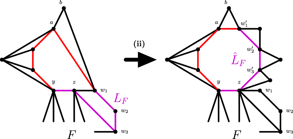
Figure 7. An example of transformation (ii) where $H_1 = K_3$
and
$H_1 = K_3$
and $H_2 = C_8$
. Observe that edges
$H_2 = C_8$
. Observe that edges $aw_1$
and
$aw_1$
and $bw_1$
are replaced by edges
$bw_1$
are replaced by edges $aw^{\prime}_1$
and
$aw^{\prime}_1$
and $bw^{\prime}_1$
.
$bw^{\prime}_1$
.
Transformation (iii): $F^2 \to F^3$
. Recall that for any
$F^2 \to F^3$
. Recall that for any $J \in \mathcal{H}(F, \hat{e}, H_1, H_2)$
, we define
$J \in \mathcal{H}(F, \hat{e}, H_1, H_2)$
, we define $v^{+}(J) \,{:\!=}\, |V(J)\setminus V(F)| = v(J) - v(F)$
and
$v^{+}(J) \,{:\!=}\, |V(J)\setminus V(F)| = v(J) - v(F)$
and $e^{+}(J) \,{:\!=}\, |E(J)\setminus E(F)| = e(J) - e(F)$
. Remove the edge
$e^{+}(J) \,{:\!=}\, |E(J)\setminus E(F)| = e(J) - e(F)$
. Remove the edge $e$
from
$e$
from $E(L'')$
(and
$E(L'')$
(and $E(L^{\prime\prime}_R)$
) to give
$E(L^{\prime\prime}_R)$
) to give $E(L'') \cap E(F) = \emptyset$
. Then
$E(L'') \cap E(F) = \emptyset$
. Then
 \begin{equation*}e^+(F \cup L_R^{\prime\prime}) = e(L_R^{\prime\prime}),\end{equation*}
and
 \begin{equation*}v^+(F \cup L_R^{\prime\prime}) = v(L_R^{\prime\prime}) - 2.\end{equation*}
If $F^2 = F \cup L_R^{\prime\prime} \in \mathcal{H}^*(F, e, H_1, H_2)$
, then transformation (iii) sets
$F^2 = F \cup L_R^{\prime\prime} \in \mathcal{H}^*(F, e, H_1, H_2)$
, then transformation (iii) sets $F^3 \,{:\!=}\, F^2$
. Otherwise we have that
$F^3 \,{:\!=}\, F^2$
. Otherwise we have that $F \cup L_R^{\prime\prime} \in \mathcal{H}(F, e, H_1, H_2)\setminus \mathcal{H}^*(F, e, H_1, H_2)$
. Let
$F \cup L_R^{\prime\prime} \in \mathcal{H}(F, e, H_1, H_2)\setminus \mathcal{H}^*(F, e, H_1, H_2)$
. Let $F^3 \,{:\!=}\, J^*$
where
$F^3 \,{:\!=}\, J^*$
where $J^*$
is any member of
$J^*$
is any member of $\mathcal{H}^*(F, e, H_1, H_2)$
and recall that, indeed,
$\mathcal{H}^*(F, e, H_1, H_2)$
and recall that, indeed, $J^*$
is a possible output of a non-degenerate iteration of the while-loop of Grow.
$J^*$
is a possible output of a non-degenerate iteration of the while-loop of Grow.
Then, in transformation (iii), we replace $F \cup L_R^{\prime\prime}$
with the graph
$F \cup L_R^{\prime\prime}$
with the graph $J^*$
. Since
$J^*$
. Since $H_2$
is (strictly)
$H_2$
is (strictly) $2$
-balanced and
$2$
-balanced and $H_1$
is (strictly) balanced with respect to
$H_1$
is (strictly) balanced with respect to $d_2(\cdot, H_2)$
, we have that
$d_2(\cdot, H_2)$
, we have that
 \begin{equation} m_2(H_1, H_2) = \frac{e_1}{v_1 - 2 + \frac{1}{m_2(H_2)}} = \frac{e_1(e_2 - 1)}{(v_1 - 2)(e_2 - 1) + v_2 - 2} = \frac{e^{+}(J^*)}{v^{+}(J^*)}. \end{equation}
Using (13) and Lemma 6.8, and that $H_2$
is (strictly)
$H_2$
is (strictly) $2$
-balanced and
$2$
-balanced and $H_1$
is (strictly) balanced with respect to
$H_1$
is (strictly) balanced with respect to $d_2(\cdot, H_2)$
, we have that
$d_2(\cdot, H_2)$
, we have that
 \begin{align*} \ & v(F^3) - v(F^2) - \frac{e(F^3) - e(F^2)}{m_2(H_1, H_2)} \\ = \ & v(J^*) - v(F \cup L_R^{\prime\prime}) - \frac{e(J^*) - e(F \cup L_R^{\prime\prime})}{m_2(H_1, H_2)} \\ = \ & v^+(J^*) - v^+(F \cup L_R^{\prime\prime}) - \frac{e^+(J^*) - e^+(F \cup L_R^{\prime\prime})}{m_2(H_1, H_2)} \\ \overset{L.6.8}{\gt } \ & v^+(J^*) - v^+(F \cup L_R^{\prime\prime}) - \frac{e^+(J^*) - e^+(J^*)\left (\frac{v^+(F \cup L_R^{\prime\prime})}{v^+(J^*)}\right )}{m_2(H_1, H_2)} \\ = \ & \left (v^+(J^*) - v^+(F \cup L_R^{\prime\prime})\right ) \left (1 - \frac{e^+(J^*)}{v^+(J^*)m_2(H_1, H_2)}\right ) \\ = \ & 0. \end{align*}
Since $v^+(J^*)$
,
$v^+(J^*)$
, $v^+(F \cup L_R^{\prime\prime})$
,
$v^+(F \cup L_R^{\prime\prime})$
, $e^+(J^*)$
,
$e^+(J^*)$
, $e^+(F \cup L_R^{\prime\prime})$
and
$e^+(F \cup L_R^{\prime\prime})$
and $m_2(H_1, H_2)$
only rely on
$m_2(H_1, H_2)$
only rely on $H_1$
and
$H_1$
and $H_2$
, there exists
$H_2$
, there exists $\delta _2 = \delta _2(H_1, H_2) \gt 0$
such that
$\delta _2 = \delta _2(H_1, H_2) \gt 0$
such that
 \begin{equation*}v(F^3) - v(F^2) - \frac {e(F^3) - e(F^2)}{m_2(H_1, H_2)} \geq \delta _2.\end{equation*}
Taking
 \begin{equation*}\kappa _2 \,{:\!=}\, \min \{1, \delta _1, \delta _2\},\end{equation*}
we see that (11) holds.
As stated earlier, Claim 6.3 follows from Claims 6.9 and 6.10. All that remains to prove Case 1 of Lemma 5.5 is to prove Lemma 6.8.
6.3 Proof of Lemma 6.8
Let $J \in \mathcal{H}(F, \hat{e}, H_1, H_2)\setminus \mathcal{H}^*(F, \hat{e}, H_1, H_2)$
. We choose the graph
$J \in \mathcal{H}(F, \hat{e}, H_1, H_2)\setminus \mathcal{H}^*(F, \hat{e}, H_1, H_2)$
. We choose the graph $J^* \in \mathcal{H}^*(F, \hat{e}, H_1, H_2)$
with the following properties.
$J^* \in \mathcal{H}^*(F, \hat{e}, H_1, H_2)$
with the following properties.
-
1) The edge of the copy
$H_{\hat{e}}$
of
$H_2$
in
$J$
attached at
$\hat{e}$
and its orientation when attached are the same as the edge of the copy
$H^*_{\hat{e}}$
of
$H_2$
in
$J^*$
attached at
$\hat{e}$
and its orientation when attached; -
2) for each
$f \in E_{J}$
, the edge of the copy
$H_f$
of
$H_1$
in
$J$
attached at
$f$
and its orientation when attached are the same as the edge of the copy
$H^*_f$
of
$H_1$
in
$J^*$
attached at
$f$
and its orientation when attached.


Then, recalling definitions from the beginning of Section 6.2, we have that $V_J = V_{J^*}$
and
$V_J = V_{J^*}$
and $E_J = E_{J^*}$
; that is,
$E_J = E_{J^*}$
; that is, $H_{\hat{e}}^{J} = H_{\hat{e}}^{J^*}$
. From now on, let
$H_{\hat{e}}^{J} = H_{\hat{e}}^{J^*}$
. From now on, let $V \,{:\!=}\, V_J$
,
$V \,{:\!=}\, V_J$
, $E \,{:\!=}\, E_J$
and
$E \,{:\!=}\, E_J$
and $H_{\hat{e}}^{-} \,{:\!=}\, H_{\hat{e}}^{J}$
. Observe for all
$H_{\hat{e}}^{-} \,{:\!=}\, H_{\hat{e}}^{J}$
. Observe for all $J' \in \mathcal{H}^*(F, \hat{e}, H_1, H_2)$
, that
$J' \in \mathcal{H}^*(F, \hat{e}, H_1, H_2)$
, that
 \begin{equation} \frac{e^{+}(J')}{v^{+}(J')} = \frac{e_1(e_2 - 1)}{(v_1 - 2)(e_2 - 1) + v_2 - 2}. \end{equation}
Hence, to prove Lemma 6.8 it suffices to show
 \begin{equation*} \frac {e^{+}(J)}{v^{+}(J)} \gt \frac {e^{+}(J^*)}{v^{+}(J^*)}. \end{equation*}
As in [Reference Marciniszyn, Skokan, Spöhel and Steger14], the intuition behind our proof is that $J^*$
can be transformed into
$J^*$
can be transformed into $J$
by successively merging the copies
$J$
by successively merging the copies $H^*_f$
of
$H^*_f$
of $H_1$
in
$H_1$
in $J^*$
with each other and vertices in
$J^*$
with each other and vertices in $H^{-}_{\hat{e}}$
. We do this in
$H^{-}_{\hat{e}}$
. We do this in $e_2 - 1$
steps, fixing carefully a total ordering of the inner edges
$e_2 - 1$
steps, fixing carefully a total ordering of the inner edges $E$
. For every edge
$E$
. For every edge $f \in E$
, we merge the attached outer copy
$f \in E$
, we merge the attached outer copy $H^*_f$
of
$H^*_f$
of $H_1$
in
$H_1$
in $J^*$
with copies of
$J^*$
with copies of $H_1$
(attached to edges preceding
$H_1$
(attached to edges preceding $f$
in our ordering) and vertices of
$f$
in our ordering) and vertices of $H^{-}_{\hat{e}}$
. Throughout, we keep track of the number of edges
$H^{-}_{\hat{e}}$
. Throughout, we keep track of the number of edges $\Delta _e(\,f)$
and the number of vertices
$\Delta _e(\,f)$
and the number of vertices $\Delta _v(\,f)$
vanishing in this process. One could hope that the
$\Delta _v(\,f)$
vanishing in this process. One could hope that the $F$
-external density of
$F$
-external density of $J$
increases in every step of this process, or, even slightly stronger, that
$J$
increases in every step of this process, or, even slightly stronger, that $\Delta _e(\,f)/ \Delta _v(\,f) \lt e^{+}(J^*)/ v^{+}(J^*)$
. This does not necessarily hold, but we will show that there exists a collection of edge-disjoint subgraphs
$\Delta _e(\,f)/ \Delta _v(\,f) \lt e^{+}(J^*)/ v^{+}(J^*)$
. This does not necessarily hold, but we will show that there exists a collection of edge-disjoint subgraphs $A_i$
of
$A_i$
of $H^{-}_{\hat{e}}$
such that, for each
$H^{-}_{\hat{e}}$
such that, for each $i$
, the edges of
$i$
, the edges of $E(A_i)$
are ‘collectively good’ for this process and every edge not belonging to one of these
$E(A_i)$
are ‘collectively good’ for this process and every edge not belonging to one of these $A_i$
is also ‘good’ for this process.
$A_i$
is also ‘good’ for this process.
Recalling definitions from the beginning of Section 6.2, let $H^{-}_f \,{:\!=}\, (U_J(\,f)\ \dot{\cup }\ f, D_J(\,f))$
denote the subgraph obtained by removing the edge
$H^{-}_f \,{:\!=}\, (U_J(\,f)\ \dot{\cup }\ f, D_J(\,f))$
denote the subgraph obtained by removing the edge $f$
from the copy
$f$
from the copy $H_f$
of
$H_f$
of $H_1$
in
$H_1$
in $J$
.
$J$
.
Later, we will carefully define a (total) ordering $\prec$
on the inner edges
$\prec$
on the inner edges $E$
.Footnote 14 For such an ordering
$E$
.Footnote 14 For such an ordering $\prec$
and each
$\prec$
and each $f \in E$
, define
$f \in E$
, define
 \begin{equation*}\Delta _E(\,f) \,{:\!=}\, D_J(\,f) \cap \left (\bigcup _{f' \prec f} D_J(\,f')\right ),\end{equation*}
and
 \begin{equation*}\Delta _V(\,f) \,{:\!=}\, U_J(\,f) \cap \left (\left (\bigcup _{f' \prec f} U_J(\,f')\right ) \cup V(H_{\hat {e}}^{-})\right ),\end{equation*}
and set $\Delta _e(\,f) \,{:\!=}\, |\Delta _E(\,f)|$
and
$\Delta _e(\,f) \,{:\!=}\, |\Delta _E(\,f)|$
and $\Delta _v(\,f) \,{:\!=}\, |\Delta _V(\,f)|$
. We emphasise here that the definition of
$\Delta _v(\,f) \,{:\!=}\, |\Delta _V(\,f)|$
. We emphasise here that the definition of $\Delta _v(\,f)$
takes into account how vertices of outer vertex sets can intersect with the inner graph
$\Delta _v(\,f)$
takes into account how vertices of outer vertex sets can intersect with the inner graph $H_{\hat{e}}^{-}$
. One can see that
$H_{\hat{e}}^{-}$
. One can see that $\Delta _e(\,f)$
(
$\Delta _e(\,f)$
( $\Delta _v(\,f)$
) is the number of edges (vertices) vanishing from
$\Delta _v(\,f)$
) is the number of edges (vertices) vanishing from $H^*_f$
when it is merged with preceding attached copies of
$H^*_f$
when it is merged with preceding attached copies of $H_1$
and
$H_1$
and $V(H_{\hat{e}}^{-})$
.
$V(H_{\hat{e}}^{-})$
.
By our choice of $J^*$
, one can quickly see that
$J^*$
, one can quickly see that
 \begin{equation} e^{+}(J) = e^{+}(J^*) - \sum _{f \in E} \Delta _e(\,f), \end{equation}
and
 \begin{equation} v^{+}(J) = v^{+}(J^*) - \sum _{f \in E} \Delta _v(\,f). \end{equation}
 \begin{equation*} \frac {e^{+}(J)}{v^{+}(J)} = \frac {e^{+}(J^*) - \sum _{f \in E} \Delta _e(\,f)}{v^{+}(J^*) - \sum _{f \in E} \Delta _v(\,f)}. \end{equation*}
Then, by Fact 4.1, to show that
 \begin{equation*} \frac {e^{+}(J)}{v^{+}(J)} \gt \frac {e^{+}(J^*)}{v^{+}(J^*)}, \end{equation*}
it suffices to prove that
 \begin{equation} \frac{\sum _{f \in E} \Delta _e(\,f)}{\sum _{f \in E} \Delta _v(\,f)} \lt \frac{e^{+}(J^*)}{v^{+}(J^*)}. \end{equation}
To show (17), we will now carefully order the edges of $E$
using an algorithm Order-Edges (Figure 8). The algorithm takes as input the graph
$E$
using an algorithm Order-Edges (Figure 8). The algorithm takes as input the graph $H_{\hat{e}}^{-} = (V \ \dot{\cup } \ \hat{e},E)$
and outputs a stack
$H_{\hat{e}}^{-} = (V \ \dot{\cup } \ \hat{e},E)$
and outputs a stack $s$
containing every edge from
$s$
containing every edge from $E$
and a collection of edge-disjoint edge sets
$E$
and a collection of edge-disjoint edge sets $E_i$
in
$E_i$
in $E$
and (not necessarily disjoint) vertex sets
$E$
and (not necessarily disjoint) vertex sets $V_i$
in
$V_i$
in $V \ \dot{\cup } \ \hat{e}$
. We take our total ordering
$V \ \dot{\cup } \ \hat{e}$
. We take our total ordering $\prec$
of
$\prec$
of $E$
to be that induced by the order in which edges of
$E$
to be that induced by the order in which edges of $E$
were placed onto the stack
$E$
were placed onto the stack $s$
(that is,
$s$
(that is, $f \prec f'$
if and only if
$f \prec f'$
if and only if $f$
was placed onto the stack
$f$
was placed onto the stack $s$
before
$s$
before $f'$
). Also, for each
$f'$
). Also, for each $i$
, we define
$i$
, we define $A_i \,{:\!=}\, (V_i, E_i)$
to be the graph on vertex set
$A_i \,{:\!=}\, (V_i, E_i)$
to be the graph on vertex set $V_i$
and edge set
$V_i$
and edge set $E_i$
and observe that
$E_i$
and observe that $A_i \subsetneq H_2$
. We will utilise this ordering and our choice of
$A_i \subsetneq H_2$
. We will utilise this ordering and our choice of $E_i$
and
$E_i$
and $V_i$
for each
$V_i$
for each $i$
, alongside that
$i$
, alongside that $H_2$
is (strictly)
$H_2$
is (strictly) $2$
-balanced and
$2$
-balanced and $H_1$
is strictly balanced with respect to
$H_1$
is strictly balanced with respect to $d_2(\cdot, H_2)$
, in order to conclude (17).
$d_2(\cdot, H_2)$
, in order to conclude (17).

Figure 8. The implementation of algorithm Order-Edges.
Let us describe algorithm Order-Edges (Figure 8) in detail. In lines 2-8, we initialise several parameters: a stack $s$
, which we will place edges of
$s$
, which we will place edges of $E$
on during our algorithm; sets
$E$
on during our algorithm; sets $E_i$
and
$E_i$
and $V_i$
for each
$V_i$
for each $i \in [\lfloor e_2/2 \rfloor ]$
,Footnote 16 which we will add edges of
$i \in [\lfloor e_2/2 \rfloor ]$
,Footnote 16 which we will add edges of $E$
and vertices of
$E$
and vertices of $V \ \dot{\cup } \ \hat{e}$
into, respectively; an index
$V \ \dot{\cup } \ \hat{e}$
into, respectively; an index $j$
, which will correspond to whichever graph
$j$
, which will correspond to whichever graph $A_j$
we consider constructing next; a set
$A_j$
we consider constructing next; a set $E'$
, which will keep track of those edges of
$E'$
, which will keep track of those edges of $E$
we have not yet placed onto the stack
$E$
we have not yet placed onto the stack $s$
. Line 9 ensures the algorithm continues until
$s$
. Line 9 ensures the algorithm continues until $E' = \emptyset$
, that is, until all the edges of
$E' = \emptyset$
, that is, until all the edges of $E$
have been placed onto
$E$
have been placed onto $s$
.
$s$
.
In line 10, we begin constructing $A_j$
by finding a pair of distinct edges in
$A_j$
by finding a pair of distinct edges in $E'$
whose outer edge sets (in
$E'$
whose outer edge sets (in $J$
) intersect. In lines 11-14, we place one of these edges,
$J$
) intersect. In lines 11-14, we place one of these edges, $f$
, onto
$f$
, onto $s$
, into
$s$
, into $E_j$
and remove it from
$E_j$
and remove it from $E'$
. We also set
$E'$
. We also set $V_j$
to be the two vertices in
$V_j$
to be the two vertices in $f$
alongside any vertices in the outer vertex set
$f$
alongside any vertices in the outer vertex set $U_J(\,f)$
that intersect
$U_J(\,f)$
that intersect $V(H^{-}_{\hat{e}})$
.
$V(H^{-}_{\hat{e}})$
.
In lines 15-20, we iteratively add onto $s$
, into
$s$
, into $E_j$
and remove from
$E_j$
and remove from $E'$
any edge
$E'$
any edge $uw \in E'$
which either connects two vertices previously added to
$uw \in E'$
which either connects two vertices previously added to $V_j$
or has an outer edge set
$V_j$
or has an outer edge set $D_J(uw)$
that intersects the collection of outer edge sets of edges previously added to
$D_J(uw)$
that intersects the collection of outer edge sets of edges previously added to $E_j$
. We also update
$E_j$
. We also update $V_j$
in each step of this process.
$V_j$
in each step of this process.
In line 21, we increment $j$
in preparation for the next check at line 10 (if we still have
$j$
in preparation for the next check at line 10 (if we still have $E' \neq \emptyset$
). If the condition in line 10 fails then in lines 23-26 we arbitrarily place the remaining edges of
$E' \neq \emptyset$
). If the condition in line 10 fails then in lines 23-26 we arbitrarily place the remaining edges of $E'$
onto the stack
$E'$
onto the stack $s$
. In line 29, we output the stack
$s$
. In line 29, we output the stack $s$
and in lines 30-32 we output each non-empty
$s$
and in lines 30-32 we output each non-empty $E_i$
and
$E_i$
and $V_i$
.
$V_i$
.
We will now argue that each proper subgraph $A_i = (V_i, E_i)$
of
$A_i = (V_i, E_i)$
of $H_2$
and each edge placed onto
$H_2$
and each edge placed onto $s$
in line 24 are ‘good’, in some sense, for us to conclude (17).
$s$
in line 24 are ‘good’, in some sense, for us to conclude (17).
For each $f \in E$
, define the graph
$f \in E$
, define the graph
 \begin{equation*}T(\,f) \,{:\!=}\, (\Delta _V(\,f) \ \dot {\cup } \ f, \Delta _E(\,f)) \subseteq H_f^- \subsetneq H_1.\end{equation*}
Observe that one or both vertices of $f$
may be isolated in
$f$
may be isolated in $T(\,f)$
. This observation will be very useful later.
$T(\,f)$
. This observation will be very useful later.
For each $i$
and
$i$
and $f \in E_i$
, define
$f \in E_i$
, define
 \begin{equation*}(V(H_{\hat {e}}^{-}))_f \,{:\!=}\, (V(H_{\hat {e}}^{-}) \cap U_J(\,f))\setminus \left (\bigcup _{\substack {f' \in E_i: \\ f' \prec f}}f' \cup \left (\bigcup _{\substack {f' \in E_i: \\ f' \prec f}} \left (V(H_{\hat {e}}^{-}) \cap U_J(\,f')\right )\right )\right ) \subseteq \Delta _V(\,f),\end{equation*}
since $(V(H_{\hat{e}}^{-}))_f$
is a subset of
$(V(H_{\hat{e}}^{-}))_f$
is a subset of $V(H_{\hat{e}}^{-}) \cap U_J(\,f)$
. One can see that
$V(H_{\hat{e}}^{-}) \cap U_J(\,f)$
. One can see that $(V(H_{\hat{e}}^{-}))_f$
consists of those vertices of
$(V(H_{\hat{e}}^{-}))_f$
consists of those vertices of $V(H_{\hat{e}}^{-})$
which are new to
$V(H_{\hat{e}}^{-})$
which are new to $V_i$
at the point when
$V_i$
at the point when $f$
is added to
$f$
is added to $E_i$
but are not contained in
$E_i$
but are not contained in $f$
. Importantly for our purposes, every vertex in
$f$
. Importantly for our purposes, every vertex in $(V(H_{\hat{e}}^{-}))_f$
is isolated in
$(V(H_{\hat{e}}^{-}))_f$
is isolated in $T(\,f)$
. Indeed, otherwise there exists
$T(\,f)$
. Indeed, otherwise there exists $k \lt i$
and
$k \lt i$
and $f'' \in E_k$
such that
$f'' \in E_k$
such that $D_J(\,f) \cap D_J(\,f'') \neq \emptyset$
and
$D_J(\,f) \cap D_J(\,f'') \neq \emptyset$
and $f$
would have been previously added to
$f$
would have been previously added to $E_k$
in line 17.
$E_k$
in line 17.
For each $f \in E$
, let
$f \in E$
, let $T'(\,f)$
be the graph obtained from
$T'(\,f)$
be the graph obtained from $T(\,f)$
by removing all isolated vertices from
$T(\,f)$
by removing all isolated vertices from $V(T(\,f))$
. Crucially for our proof, since vertices of
$V(T(\,f))$
. Crucially for our proof, since vertices of $f$
may be isolated in
$f$
may be isolated in $T(\,f)$
, one or more of them may not belong to
$T(\,f)$
, one or more of them may not belong to $V(T'(\,f))$
. Further, no vertex of
$V(T'(\,f))$
. Further, no vertex of $(V(H_{\hat{e}}^{-}))_f$
is contained in
$(V(H_{\hat{e}}^{-}))_f$
is contained in $V(T'(\,f))$
.
$V(T'(\,f))$
.
For all $f \in E$
with
$f \in E$
with $\Delta _e(\,f) \geq 1$
, since
$\Delta _e(\,f) \geq 1$
, since $T'(\,f) \subsetneq H_1$
and
$T'(\,f) \subsetneq H_1$
and $H_1$
is strictly balanced with respect to
$H_1$
is strictly balanced with respect to $d_2(\cdot, H_2)$
, we have that
$d_2(\cdot, H_2)$
, we have that
 \begin{equation} m_2(H_1, H_2) \gt d_2(T'(\,f), H_2) = \frac{|E(T'(\,f))|}{|V(T'(\,f))| - 2 + \frac{1}{m_2(H_2)}}. \end{equation}
Recall (13), that is,
 \begin{equation*}m_2(H_1, H_2) = \frac {e^+(J^*)}{v^+(J^*)}.\end{equation*}
We now make the key observation of our proof: Since vertices of $f$
may be isolated in
$f$
may be isolated in $T(\,f)$
, and so not contained in
$T(\,f)$
, and so not contained in $V(T'(\,f))$
, and no vertex of
$V(T'(\,f))$
, and no vertex of $(V(H_{\hat{e}}^{-}))_f$
is contained in
$(V(H_{\hat{e}}^{-}))_f$
is contained in $V(T'(\,f))$
, we have that
$V(T'(\,f))$
, we have that
 \begin{equation} |V(T'(\,f))| \leq \Delta _v(\,f) + |f \cap V(T'(\,f))| - |(V(H_{\hat{e}}))_f|. \end{equation}
Hence, from (18) and (19) we have that
 \begin{align} \Delta _e(\,f) = \ &|E(T'(\,f))| \nonumber \\ \lt \ &m_2(H_1, H_2)\left (\Delta _v(\,f) - (2 - |f \cap V(T'(\,f))|) - |(V(H_{\hat{e}}^{-}))_f| + \frac{1}{m_2(H_2)}\right ). \end{align}
Edges $f$
such that
$f$
such that $|f \cap V(T'(\,f))| = 2$
will be, in some sense, ‘bad’ for us when trying to conclude (17). Indeed, if
$|f \cap V(T'(\,f))| = 2$
will be, in some sense, ‘bad’ for us when trying to conclude (17). Indeed, if $|(V(H_{\hat{e}}^{-}))_f| = 0$
then we may have that
$|(V(H_{\hat{e}}^{-}))_f| = 0$
then we may have that $\frac{\Delta _e(\,f)}{\Delta _v(\,f)} \geq m_2(H_1, H_2) = \frac{e^{+}(J^*)}{v^{+}(J^*)}$
, by (13). However, edges
$\frac{\Delta _e(\,f)}{\Delta _v(\,f)} \geq m_2(H_1, H_2) = \frac{e^{+}(J^*)}{v^{+}(J^*)}$
, by (13). However, edges $f$
such that
$f$
such that $|f \cap V(T'(\,f))| \in \{0,1\}$
will be, in some sense, ‘good’ for us when trying to conclude (17). Indeed, since
$|f \cap V(T'(\,f))| \in \{0,1\}$
will be, in some sense, ‘good’ for us when trying to conclude (17). Indeed, since $m_2(H_2) \geq 1$
, we have for such edges
$m_2(H_2) \geq 1$
, we have for such edges $f$
that
$f$
that $\frac{\Delta _e(\,f)}{\Delta _v(\,f)} \lt m_2(H_1, H_2) = \frac{e^{+}(J^*)}{v^{+}(J^*)}$
.
$\frac{\Delta _e(\,f)}{\Delta _v(\,f)} \lt m_2(H_1, H_2) = \frac{e^{+}(J^*)}{v^{+}(J^*)}$
.
We show in the following claim that our choice of ordering $\prec$
, our choice of each
$\prec$
, our choice of each $A_i$
and the fact that
$A_i$
and the fact that $H_2$
is (strictly)
$H_2$
is (strictly) $2$
-balanced ensure that for each
$2$
-balanced ensure that for each $i$
there are enough ‘good’ edges in
$i$
there are enough ‘good’ edges in $A_i$
to compensate for any ‘bad’ edges that may appear in
$A_i$
to compensate for any ‘bad’ edges that may appear in $A_i$
.
$A_i$
.
Claim 6.11.
For each $i$
,
$i$
,
 \begin{equation*} \sum _{f \in E_i} \Delta _e(\,f) \lt m_2(H_1, H_2) \sum _{f \in E_i} \Delta _v(\,f). \end{equation*}
Proof. Fix $i$
. Firstly, as observed before, each
$i$
. Firstly, as observed before, each $A_i$
is a non-empty subgraph of
$A_i$
is a non-empty subgraph of $H_2$
. Moreover,
$H_2$
. Moreover, $|E_i| \geq 2$
(by the condition in line 10). Since
$|E_i| \geq 2$
(by the condition in line 10). Since $H_2$
is (strictly)
$H_2$
is (strictly) $2$
-balanced, we have that
$2$
-balanced, we have that
 \begin{equation} m_2(H_2) \geq d_2(A_i) = \frac{|E_i| - 1}{|V_i| - 2}. \end{equation}
Now let us consider $\Delta _e(\,f)$
for each
$\Delta _e(\,f)$
for each $f \in E_i$
. For the edge
$f \in E_i$
. For the edge $f$
added in line 12, observe that
$f$
added in line 12, observe that $\Delta _e(\,f) = 0$
. Indeed, otherwise
$\Delta _e(\,f) = 0$
. Indeed, otherwise $\Delta _e(\,f) \geq 1$
, and there exists
$\Delta _e(\,f) \geq 1$
, and there exists $k \lt i$
such that
$k \lt i$
such that $D_J(\,f) \cap \left (\bigcup _{f' \in E_k}D_J(\,f')\right ) \neq \emptyset$
. That is,
$D_J(\,f) \cap \left (\bigcup _{f' \in E_k}D_J(\,f')\right ) \neq \emptyset$
. That is, $f$
would have been added to
$f$
would have been added to $E_k$
in line 17 previously in the algorithm. Since
$E_k$
in line 17 previously in the algorithm. Since $(V(H_{\hat{e}}^{-}))_f \subseteq \Delta _V(\,f)$
, we have that
$(V(H_{\hat{e}}^{-}))_f \subseteq \Delta _V(\,f)$
, we have that
 \begin{equation} \Delta _e(\,f) = 0 \leq m_2(H_1, H_2)\left (\Delta _v(\,f) - |(V(H_{\hat{e}}^{-}))_f|\right ). \end{equation}
Now, for each edge added in line 17, either $v,w \in V_i$
when
$v,w \in V_i$
when $uw$
was added to
$uw$
was added to $E_i$
, or we had
$E_i$
, or we had $D_J(uw) \cap \left (\bigcup _{\substack{f' \in E_i: \\ f' \prec uw}}D_J(\,f')\right ) \neq \emptyset$
, that is,
$D_J(uw) \cap \left (\bigcup _{\substack{f' \in E_i: \\ f' \prec uw}}D_J(\,f')\right ) \neq \emptyset$
, that is, $\Delta _e(uw) \geq 1$
, and at least one of
$\Delta _e(uw) \geq 1$
, and at least one of $u$
,
$u$
, $w$
did not belong to
$w$
did not belong to $V_i$
when
$V_i$
when $uw$
was added to
$uw$
was added to $E_i$
. In the former case, if
$E_i$
. In the former case, if $\Delta _e(uw) \geq 1$
, then by (20) and that
$\Delta _e(uw) \geq 1$
, then by (20) and that $-(2 - |f \cap V(T'(\,f))|) \leq 0$
, we have that
$-(2 - |f \cap V(T'(\,f))|) \leq 0$
, we have that
 \begin{equation} \Delta _e(uw) \lt m_2(H_1, H_2)\left (\Delta _v(uw) - |(V(H_{\hat{e}}^{-}))_{uw}| + \frac{1}{m_2(H_2)}\right ). \end{equation}
Observe that (23) also holds when $\Delta _{e}(uw) = 0$
. In the latter case, observe that for all
$\Delta _{e}(uw) = 0$
. In the latter case, observe that for all $k \lt i$
, we must have
$k \lt i$
, we must have $D_{J}(uw) \cap \left (\bigcup _{f \in E_k}D_J(\,f)\right ) = \emptyset$
. Indeed, otherwise
$D_{J}(uw) \cap \left (\bigcup _{f \in E_k}D_J(\,f)\right ) = \emptyset$
. Indeed, otherwise $uw$
would have been added to some
$uw$
would have been added to some $E_k$
in line 17. Combining this with knowing that at least one of
$E_k$
in line 17. Combining this with knowing that at least one of $u$
,
$u$
, $w$
did not belong to
$w$
did not belong to $V_i$
before
$V_i$
before $uw$
was added to
$uw$
was added to $E_i$
, we must have that one or both of
$E_i$
, we must have that one or both of $u$
,
$u$
, $w$
are isolated in
$w$
are isolated in $T(uw)$
. That is, one or both do not belong to
$T(uw)$
. That is, one or both do not belong to $T'(uw)$
, and so
$T'(uw)$
, and so $|uw \cap V(T'(uw))| \in \{0,1\}$
. Thus, since
$|uw \cap V(T'(uw))| \in \{0,1\}$
. Thus, since $\Delta _e(uw) \geq 1$
, by (20) we have that
$\Delta _e(uw) \geq 1$
, by (20) we have that
 \begin{equation} \Delta _e(uw) \lt m_2(H_1, H_2)\left (\Delta _v(uw) - 1 - |(V(H_{\hat{e}}^{-}))_{uw}| + \frac{1}{m_2(H_2)}\right ), \end{equation}
if $|uw \cap V(T'(uw))| = 1$
, and
$|uw \cap V(T'(uw))| = 1$
, and
 \begin{equation} \Delta _e(uw) \lt m_2(H_1, H_2)\left (\Delta _v(uw) - 2 - |(V(H_{\hat{e}}^{-}))_{uw}| + \frac{1}{m_2(H_2)}\right ), \end{equation}
if $|uw \cap V(T'(uw))| = 0$
.
$|uw \cap V(T'(uw))| = 0$
.
In conclusion, except for the two vertices in the edge added in line 12, every time a new vertex $x$
was added to
$x$
was added to $V_i$
when some edge
$V_i$
when some edge $f$
was added to
$f$
was added to $E_i$
, either
$E_i$
, either $x \in (V(H_{\hat{e}}^{-}))_{f}$
, or
$x \in (V(H_{\hat{e}}^{-}))_{f}$
, or $x \in f$
and (24) or (25) held, dependent on whether one or both of the vertices in
$x \in f$
and (24) or (25) held, dependent on whether one or both of the vertices in $f$
were new to
$f$
were new to $V_i$
. Indeed,
$V_i$
. Indeed, $x$
was isolated in
$x$
was isolated in $T(\,f)$
. Moreover, after the two vertices in the edge added in line 12 there are
$T(\,f)$
. Moreover, after the two vertices in the edge added in line 12 there are $|V_i| - 2$
vertices added to
$|V_i| - 2$
vertices added to $V_i$
.
$V_i$
.
Hence, by (22)-(25), we have that
 \begin{equation} \sum _{f \in E_i} \Delta _e(\,f) \lt m_2(H_1, H_2)\left (\sum _{f \in E_i} \Delta _v(\,f) - (|V_i| - 2) + \frac{|E_i| - 1}{m_2(H_2)}\right ). \end{equation}
By (21),
 \begin{equation} - (|V_i| - 2) + \frac{|E_i| - 1}{m_2(H_2)} \leq 0. \end{equation}
Thus, by (26) and (27), we have that
 \begin{equation*}\sum _{f \in E_i} \Delta _e(\,f) \lt m_2(H_1, H_2) \sum _{f \in E_i} \Delta _v(\,f),\end{equation*}
as desired.
Claim 6.12.
For each edge $f$
placed onto
$f$
placed onto $s$
in line 24, we have
$s$
in line 24, we have $\Delta _e(\,f) = 0$
.
$\Delta _e(\,f) = 0$
.
Proof. Assume not. Then $\Delta _e(\,f) \geq 1$
for some edge
$\Delta _e(\,f) \geq 1$
for some edge $f$
placed onto
$f$
placed onto $s$
in line 24. Observe that
$s$
in line 24. Observe that $D_J(\,f) \cap \left (\bigcup _{f'' \in E_i} D_J(\,f'')\right ) = \emptyset$
for any
$D_J(\,f) \cap \left (\bigcup _{f'' \in E_i} D_J(\,f'')\right ) = \emptyset$
for any $i$
, otherwise
$i$
, otherwise $f$
would have been added to some
$f$
would have been added to some $E_i$
in line 17 previously.
$E_i$
in line 17 previously.
Thus we must have that $D_J(\,f) \cap D_J(\,f') \neq \emptyset$
for some edge
$D_J(\,f) \cap D_J(\,f') \neq \emptyset$
for some edge $f' \neq f$
where
$f' \neq f$
where $f'$
was placed onto
$f'$
was placed onto $s$
also in line 24. But then
$s$
also in line 24. But then $f$
and
$f$
and $f'$
satisfy the condition in line 10 and would both be contained in some
$f'$
satisfy the condition in line 10 and would both be contained in some $E_i$
, contradicting that
$E_i$
, contradicting that $f$
was placed onto
$f$
was placed onto $s$
in line 24.
$s$
in line 24.
Since $J \in \mathcal{H}(F, \hat{e}, H_1, H_2)\setminus \mathcal{H}^*(F, \hat{e}, H_1, H_2)$
, we must have that
$J \in \mathcal{H}(F, \hat{e}, H_1, H_2)\setminus \mathcal{H}^*(F, \hat{e}, H_1, H_2)$
, we must have that $\Delta _v(\,f) \geq 1$
for some
$\Delta _v(\,f) \geq 1$
for some $f \in E$
. Thus, if
$f \in E$
. Thus, if $\Delta _e(\,f) = 0$
for all
$\Delta _e(\,f) = 0$
for all $f \in E$
then (17) holds trivially. If
$f \in E$
then (17) holds trivially. If $\Delta _e(\,f) \geq 1$
for some
$\Delta _e(\,f) \geq 1$
for some $f \in E$
, then
$f \in E$
, then $E_1 \neq \emptyset$
and
$E_1 \neq \emptyset$
and $A_1$
is a non-empty subgraph of
$A_1$
is a non-empty subgraph of $H_{\hat{e}}^{-}$
. Then, by (13) and Claims 6.11 and 6.12, we have that
$H_{\hat{e}}^{-}$
. Then, by (13) and Claims 6.11 and 6.12, we have that
 \begin{align*} \frac{\sum _{f \in E} \Delta _e(\,f)}{\sum _{f \in E} \Delta _v(\,f)} & = \frac{\sum _i\sum _{f \in E_i} \Delta _e(\,f) + \sum _{f \in E\setminus \cup _i E_i} \Delta _e(\,f)}{\sum _{f \in E} \Delta _v(\,f)} \\[3pt] & \lt \frac{m_2(H_1, H_2)\sum _i\sum _{f \in E_i} \Delta _v(\,f)}{\sum _i\sum _{f \in E_i} \Delta _v(\,f)} \\[3pt] & = m_2(H_1, H_2) \\ & = \frac{e^{+}(J^*)}{v^{+}(J^*)}. \end{align*}
Thus (17) holds and we are done.
7. Case 2:
$m_2(H_1, H_2) = m_2(H_2)$
.

In this section we prove Lemma 5.5 when $m_2(H_1) = m_2(H_2)$
. Our proof follows that of Case 1 significantly, but uses a different algorithm Grow-Alt. All definitions and notation are the same as previously unless otherwise stated.
$m_2(H_1) = m_2(H_2)$
. Our proof follows that of Case 1 significantly, but uses a different algorithm Grow-Alt. All definitions and notation are the same as previously unless otherwise stated.
For any graph $F$
and edge
$F$
and edge $e \in E(F)$
, we say that
$e \in E(F)$
, we say that $e$
is eligible for extension in Grow-Alt if it satisfies
$e$
is eligible for extension in Grow-Alt if it satisfies
 \begin{equation*}\nexists L \in \mathcal {L}_F, R \in \mathcal {R}_F \ \text {s.t.} \ E(L) \cap E(R) = \{e\}.\end{equation*}
We note here that this is substantially different to Case 1; indeed, the set $\mathcal{C}^*$
will not feature in what follows. Algorithm Grow-Alt is shown in Figure 9. As with Grow, it has input
$\mathcal{C}^*$
will not feature in what follows. Algorithm Grow-Alt is shown in Figure 9. As with Grow, it has input $G' \subseteq G$
, the graph that Asym-Edge-Col got stuck on. Grow-Alt operates in a similar way to Grow. In line 14, the function Eligible-Edge-Alt is called which maps
$G' \subseteq G$
, the graph that Asym-Edge-Col got stuck on. Grow-Alt operates in a similar way to Grow. In line 14, the function Eligible-Edge-Alt is called which maps $F_i$
to an edge
$F_i$
to an edge $e \in E(F_i)$
which is eligible for extension in Grow-Alt. As with Eligible-Edge in Case 1, this edge
$e \in E(F_i)$
which is eligible for extension in Grow-Alt. As with Eligible-Edge in Case 1, this edge $e$
is selected to be unique up to isomorphism. We then apply a new procedure Extend which attaches either a graph
$e$
is selected to be unique up to isomorphism. We then apply a new procedure Extend which attaches either a graph $L \in \mathcal{L}_{G^{\prime}}$
or a graph
$L \in \mathcal{L}_{G^{\prime}}$
or a graph $R \in \mathcal{R}_{G^{\prime}}$
that contains
$R \in \mathcal{R}_{G^{\prime}}$
that contains $e$
to
$e$
to $F_i$
. As in Case 1, because the condition in line 6 of Asym-Edge-Col fails,
$F_i$
. As in Case 1, because the condition in line 6 of Asym-Edge-Col fails, $G' \in \mathcal{C}$
.Footnote 17
$G' \in \mathcal{C}$
.Footnote 17

Figure 9. The implementation of algorithm Grow-Alt.
We now show that the number of edges of $F_i$
increases by at least one and that Grow-Alt operates as desired with a result analogous to Claim 6.1.
$F_i$
increases by at least one and that Grow-Alt operates as desired with a result analogous to Claim 6.1.
Claim 7.1.
Algorithm Grow-Alt terminates without error on any input graph $G' \in \mathcal{C}$
that is not
$G' \in \mathcal{C}$
that is not $(H_1, H_2)$
-sparse or not an
$(H_1, H_2)$
-sparse or not an $\hat{\mathcal{A}}$
-graph.
Footnote 18 Moreover, for every iteration
$\hat{\mathcal{A}}$
-graph.
Footnote 18 Moreover, for every iteration $i$
of the while-loop, we have
$i$
of the while-loop, we have $e(F_{i+1}) \gt e(F_i)$
.
$e(F_{i+1}) \gt e(F_i)$
.
Proof. The special cases in lines 2-9 and the assignments in lines 10 and 11 operate successfully for the exact same reasons as given in the proof of Claim 6.1.
Next, we show that the call to Eligible-Edge-Alt in line 14 is always successful. Indeed, suppose for a contradiction that no edge in $F_i$
is eligible for extension in Grow-Alt for some
$F_i$
is eligible for extension in Grow-Alt for some $i \geq 0$
. Then for every edge
$i \geq 0$
. Then for every edge $e \in E(F_i)$
there exist
$e \in E(F_i)$
there exist $L \in \mathcal{L}_{F_i}$
and
$L \in \mathcal{L}_{F_i}$
and $R \in \mathcal{R}_{F_i}$
s.t.
$R \in \mathcal{R}_{F_i}$
s.t. $E(L) \cap E(R) = \{e\}$
, by definition. Hence
$E(L) \cap E(R) = \{e\}$
, by definition. Hence $F \in \mathcal{C}$
. Recall that
$F \in \mathcal{C}$
. Recall that $H_1$
and
$H_1$
and $H_2$
satisfy the criteria of Conjecture 1.8. Hence
$H_2$
satisfy the criteria of Conjecture 1.8. Hence $H_1$
and
$H_1$
and $H_2$
are strictly
$H_2$
are strictly $2$
-balanced and
$2$
-balanced and $m_2(H_1) = m_2(H_2) \gt 1$
. Then, by Lemma 4.2, we have that
$m_2(H_1) = m_2(H_2) \gt 1$
. Then, by Lemma 4.2, we have that $H_1$
and
$H_1$
and $H_2$
are both
$H_2$
are both $2$
-connected. Hence
$2$
-connected. Hence $F_i$
is
$F_i$
is $2$
-connected by construction. However, our choice of
$2$
-connected by construction. However, our choice of $F_0$
in line 11 guarantees that
$F_0$
in line 11 guarantees that $F_i$
is not in
$F_i$
is not in $\hat{\mathcal{A}}$
. Indeed, the edge
$\hat{\mathcal{A}}$
. Indeed, the edge $e$
selected in line 10 satisfying
$e$
selected in line 10 satisfying $|\mathcal{S}_{G^{\prime}}(e)| = 0$
is an edge of
$|\mathcal{S}_{G^{\prime}}(e)| = 0$
is an edge of $F_0$
and
$F_0$
and $F_0 \subseteq F_i \subseteq G'$
. Thus, by the definition of
$F_0 \subseteq F_i \subseteq G'$
. Thus, by the definition of $\hat{\mathcal{A}}$
and that
$\hat{\mathcal{A}}$
and that $m_2(H_1) = m_2(H_2)$
, we have that
$m_2(H_1) = m_2(H_2)$
, we have that $m(F_i) \gt m_2(H_1, H_2) + \varepsilon$
.
$m(F_i) \gt m_2(H_1, H_2) + \varepsilon$
.
Thus, there exists a non-empty graph $\tilde{F} \subseteq F_i$
with
$\tilde{F} \subseteq F_i$
with $d(\tilde{F}) = m(F_i)$
such that
$d(\tilde{F}) = m(F_i)$
such that
 \begin{align*} \lambda (\tilde{F}) = v(\tilde{F}) - \frac{e(\tilde{F})}{m_2(H_1, H_2)} & = e(\tilde{F})\left (\frac{1}{m(F_i)} - \frac{1}{m_2(H_1, H_2)}\right ) \\ & \lt e(\tilde{F})\left (\frac{1}{m_2(H_1, H_2) + \varepsilon } - \frac{1}{m_2(H_1, H_2)}\right ) = -\gamma e(\tilde{F}) \leq -\gamma . \end{align*}
Thus Grow terminates in line 13 without calling Eligible-Edge-Alt. Thus every call that is made to Eligible-Edge-Alt is successful and returns an edge $e$
. Since
$e$
. Since $G' \in \mathcal{C}$
, the call to Extend
$G' \in \mathcal{C}$
, the call to Extend $(F_i, e, G')$
is also successful and thus there exist suitable graphs
$(F_i, e, G')$
is also successful and thus there exist suitable graphs $L \in \mathcal{L}_{G^{\prime}}$
and
$L \in \mathcal{L}_{G^{\prime}}$
and $R \in \mathcal{R}_{G^{\prime}}$
such that
$R \in \mathcal{R}_{G^{\prime}}$
such that $E(L) \cap E(R) = \{e\}$
, that is, line 2 is successful.
$E(L) \cap E(R) = \{e\}$
, that is, line 2 is successful.
It remains to show that for every iteration $i$
of the while-loop, we have
$i$
of the while-loop, we have $e(F_{i+1}) \gt e(F_i)$
. Since
$e(F_{i+1}) \gt e(F_i)$
. Since $e$
is eligible for extension in Grow-Alt for
$e$
is eligible for extension in Grow-Alt for $F_i$
and
$F_i$
and $E(L) \cap E(R) = \{e\}$
, we must have that either
$E(L) \cap E(R) = \{e\}$
, we must have that either $L \nsubseteq F_i$
or
$L \nsubseteq F_i$
or $R \nsubseteq F_i$
. Hence Extend outputs
$R \nsubseteq F_i$
. Hence Extend outputs $F' \,{:\!=}\, F \cup L$
such that
$F' \,{:\!=}\, F \cup L$
such that $e(F_{i+1}) = e(F') \gt e(F_i)$
or
$e(F_{i+1}) = e(F') \gt e(F_i)$
or $F' \,{:\!=}\, F \cup R$
such that
$F' \,{:\!=}\, F \cup R$
such that $e(F_{i+1}) = e(F') \gt e(F_i)$
.
$e(F_{i+1}) = e(F') \gt e(F_i)$
.
We consider the evolution of $F_i$
now in more detail. We call iteration
$F_i$
now in more detail. We call iteration $i$
of the while-loop in algorithm Grow-Alt non-degenerate (See Figure 10) if the following hold:
$i$
of the while-loop in algorithm Grow-Alt non-degenerate (See Figure 10) if the following hold:
-
• If
$L \nsubseteq F_i$
(that is, line 3 is true), then in line 4 we have
$V(F_i) \cap V(L) = e$
; -
• If
$L \subseteq F_i$
(that is, line 3 is false), then in line 6 we have
$V(F_i) \cap V(R) = e$
.


Figure 10. A graph $F_3$
resulting from three non-degenerate iterations for
$F_3$
resulting from three non-degenerate iterations for $H_1 = K_3$
and
$H_1 = K_3$
and $H_2 = K_{3,3}$
.
$H_2 = K_{3,3}$
.
Otherwise, we call iteration $i$
degenerate. Note that, in non-degenerate iterations
$i$
degenerate. Note that, in non-degenerate iterations $i$
, there are only a constant number of graphs that
$i$
, there are only a constant number of graphs that $F_{i+1}$
can be for any given
$F_{i+1}$
can be for any given $F_i$
; indeed, Eligible-Edge-Alt determines the exact position where to attach
$F_i$
; indeed, Eligible-Edge-Alt determines the exact position where to attach $L$
or
$L$
or $R$
(recall that the edge
$R$
(recall that the edge $e$
found by Eligible-Edge-Alt(
$e$
found by Eligible-Edge-Alt( $F_i$
) is unique up to isomorphism of
$F_i$
) is unique up to isomorphism of $F_i$
).
$F_i$
).
We now prove a result analogous to Claim 6.2 for Grow-Alt.
Claim 7.2.
If iteration $i$
of the while-loop in procedure Grow-Alt is non-degenerate, we have
$i$
of the while-loop in procedure Grow-Alt is non-degenerate, we have
 \begin{equation*}\lambda (F_{i+1}) = \lambda (F_i).\end{equation*}
Proof. In a non-degenerate iteration, we either add $v_2 - 2$
vertices and
$v_2 - 2$
vertices and $e_2 - 1$
edges for the copy
$e_2 - 1$
edges for the copy $L$
of
$L$
of $H_2$
to
$H_2$
to $F_i$
or add
$F_i$
or add $v_1 - 2$
vertices and
$v_1 - 2$
vertices and $e_1 - 1$
edges for the copy
$e_1 - 1$
edges for the copy $R$
of
$R$
of $H_1$
to
$H_1$
to $F_i$
. In the former case,
$F_i$
. In the former case,
 \begin{align*} \lambda (F_{i+1}) - \lambda (F_i) & = v_2 - 2 - \frac{e_2 - 1}{m_2(H_1,H_2)} \\ & = v_2 - 2 - \frac{e_2 - 1}{m_2(H_2)} \\ & = 0, \end{align*}
where the second equality follows from $m_2(H_1,H_2) = m_2(H_2)$
(see Proposition 1.7) and the last equality follows from
$m_2(H_1,H_2) = m_2(H_2)$
(see Proposition 1.7) and the last equality follows from $H_2$
being (strictly)
$H_2$
being (strictly) $2$
-balanced.
$2$
-balanced.
In the latter case,
 \begin{align*} \lambda (F_{i+1}) - \lambda (F_i) & = v_1 - 2 - \frac{e_1 - 1}{m_2(H_1,H_2)} \\ & = v_1 - 2 - \frac{e_1 - 1}{m_2(H_1)} \\ & = 0. \end{align*}
where the second equality follows from $m_2(H_1,H_2) = m_2(H_1)$
(see Proposition 1.7) and the last equality follows from
$m_2(H_1,H_2) = m_2(H_1)$
(see Proposition 1.7) and the last equality follows from $H_1$
being (strictly)
$H_1$
being (strictly) $2$
-balanced.
$2$
-balanced.
As in Case 1, when we have a degenerate iteration $i$
, the structure of
$i$
, the structure of $F_{i+1}$
depends not just on
$F_{i+1}$
depends not just on $F_i$
but also on the structure of
$F_i$
but also on the structure of $G'$
. Indeed, if
$G'$
. Indeed, if $F_i$
is extended by a copy
$F_i$
is extended by a copy $L$
of
$L$
of $H_2$
in line 4 of Extend, then
$H_2$
in line 4 of Extend, then $L$
could intersect
$L$
could intersect $F_i$
in a multitude of ways. Moreover, there may be several copies of
$F_i$
in a multitude of ways. Moreover, there may be several copies of $H_2$
that satisfy the condition in line 2 of Extend. One could say the same for graphs added in line 6 of Extend. Thus, as in Case 1, degenerate iterations cause us difficulties since they enlarge the family of graphs algorithm Grow-Alt can return. However, we will show that at most a constant number of degenerate iterations can happen before algorithm Grow-Alt terminates, allowing us to bound from above sufficiently well the number of non-isomorphic graphs Grow-Alt can return. Pivotal in proving this is the following claim, analogous to Claim 6.3.
$H_2$
that satisfy the condition in line 2 of Extend. One could say the same for graphs added in line 6 of Extend. Thus, as in Case 1, degenerate iterations cause us difficulties since they enlarge the family of graphs algorithm Grow-Alt can return. However, we will show that at most a constant number of degenerate iterations can happen before algorithm Grow-Alt terminates, allowing us to bound from above sufficiently well the number of non-isomorphic graphs Grow-Alt can return. Pivotal in proving this is the following claim, analogous to Claim 6.3.
Claim 7.3.
There exists a constant $\kappa = \kappa (H_1,H_2) \gt 0$
such that if iteration
$\kappa = \kappa (H_1,H_2) \gt 0$
such that if iteration $i$
of the while-loop in procedure Grow is degenerate then we have
$i$
of the while-loop in procedure Grow is degenerate then we have
 \begin{equation*}\lambda (F_{i+1}) \leq \lambda (F_i) - \kappa .\end{equation*}
Compared to the proof of Claim 6.3, the proof of Claim 7.3 is relatively straightforward.
Proof. Let $F \,{:\!=}\, F_i$
be the graph before the operation in line 15 (of Grow-Alt) is carried out and let
$F \,{:\!=}\, F_i$
be the graph before the operation in line 15 (of Grow-Alt) is carried out and let $F' \,{:\!=}\, F_{i+1}$
be the output from line 15. We aim to show there exists a constant
$F' \,{:\!=}\, F_{i+1}$
be the output from line 15. We aim to show there exists a constant $\kappa = \kappa (H_1, H_2) \gt 0$
such that
$\kappa = \kappa (H_1, H_2) \gt 0$
such that
 \begin{equation*} \lambda (F) - \lambda (F') = v(F) - v(F') - \frac {e(F) - e(F')}{m_2(H_1, H_2)} \geq \kappa \end{equation*}
whether Extend attached a graph $L \in \mathcal{L}_{G^{\prime}}$
or
$L \in \mathcal{L}_{G^{\prime}}$
or $R \in \mathcal{R}_{G^{\prime}}$
to
$R \in \mathcal{R}_{G^{\prime}}$
to $F$
. We need only consider the case when
$F$
. We need only consider the case when $L \in \mathcal{L}_{G^{\prime}}$
is the graph added by Extend in this non-degenerate iteration
$L \in \mathcal{L}_{G^{\prime}}$
is the graph added by Extend in this non-degenerate iteration $i$
of the while-loop, as the proof of the
$i$
of the while-loop, as the proof of the $R \in \mathcal{R}_{G^{\prime}}$
case is identical. Let
$R \in \mathcal{R}_{G^{\prime}}$
case is identical. Let $V_{L'} \,{:\!=}\, V(F) \cap V(L)$
and
$V_{L'} \,{:\!=}\, V(F) \cap V(L)$
and $E_{L'} \,{:\!=}\, E(F) \cap E(L)$
and set
$E_{L'} \,{:\!=}\, E(F) \cap E(L)$
and set $v_{L'} \,{:\!=}\, |V_{L'}|$
and
$v_{L'} \,{:\!=}\, |V_{L'}|$
and $e_{L'} \,{:\!=}\, |E_{L'}|$
. Let
$e_{L'} \,{:\!=}\, |E_{L'}|$
. Let $L'$
be the graph on vertex set
$L'$
be the graph on vertex set $V_{L'}$
and edge set
$V_{L'}$
and edge set $E_{L'}$
. By Claim 7.1, we have
$E_{L'}$
. By Claim 7.1, we have $e(F') \gt e(F)$
, hence
$e(F') \gt e(F)$
, hence $L'$
is a proper subgraph of
$L'$
is a proper subgraph of $H_2$
. Also, observe that since iteration
$H_2$
. Also, observe that since iteration $i$
was degenerate, we must have that
$i$
was degenerate, we must have that $v_{L'} \geq 3$
. Let
$v_{L'} \geq 3$
. Let $F_{\hat{L}}$
be the graph produced by a non-degenerate iteration at
$F_{\hat{L}}$
be the graph produced by a non-degenerate iteration at $e$
with a copy
$e$
with a copy $\hat{L}$
of
$\hat{L}$
of $H_2$
, that is,
$H_2$
, that is, $F_{\hat{L}} \,{:\!=}\, F \cup \hat{L}$
and
$F_{\hat{L}} \,{:\!=}\, F \cup \hat{L}$
and $V(F) \cap V(\hat{L}) = e$
. Our strategy is to compare
$V(F) \cap V(\hat{L}) = e$
. Our strategy is to compare $F'$
with
$F'$
with $F_{\hat{L}}$
. By Claim 7.2,
$F_{\hat{L}}$
. By Claim 7.2, $\lambda (F) = \lambda (F_{\hat{L}})$
. Thus, since
$\lambda (F) = \lambda (F_{\hat{L}})$
. Thus, since $m_2(H_1, H_2) = m_2(H_2)$
, we have
$m_2(H_1, H_2) = m_2(H_2)$
, we have
 \begin{align} \lambda (F) - \lambda (F') &= \lambda (F_{\hat{L}}) - \lambda (F') \nonumber\\[3pt]&= v_2 - 2 - (v_2 - v_{L'}) - \frac{(e_2 - 1) - (e_2 - e_{L'})}{m_2(H_1, H_2)}\nonumber\\& = v_{L'} - 2 - \frac{e_{L'} - 1}{m_2(H_1, H_2)}. \end{align}
If $e_{L'} = 1$
, then since
$e_{L'} = 1$
, then since $v_{L'} \geq 3$
we have
$v_{L'} \geq 3$
we have $\lambda (F) - \lambda (F') \geq 1$
. So assume
$\lambda (F) - \lambda (F') \geq 1$
. So assume $e_{L'} \geq 2$
. Since
$e_{L'} \geq 2$
. Since $H_2$
is strictly
$H_2$
is strictly $2$
-balanced and
$2$
-balanced and $L'$
is a proper subgraph of
$L'$
is a proper subgraph of $H_2$
with
$H_2$
with $e_{L'} \geq 2$
(that is,
$e_{L'} \geq 2$
(that is, $L'$
is not an edge), we have that
$L'$
is not an edge), we have that
 \begin{equation} \frac{v_{L'} - 2}{e_{L'} - 1} \gt \frac{1}{m_2(H_2)}. \end{equation}
Using (28), (29) and that $e_{L'} \geq 2$
and
$e_{L'} \geq 2$
and $m_2(H_1, H_2) = m_2(H)$
, we have
$m_2(H_1, H_2) = m_2(H)$
, we have
 \begin{equation*} \lambda (F) - \lambda (F') = (e_{L'} - 1)\left (\frac {v_{L'} - 2}{e_{L'} - 1} - \frac {1}{m_2(H_2)}\right ) \gt 0. \end{equation*}
Letting $\delta \,{:\!=}\, \frac{1}{2} \min \!\left \{(e_{L'} - 1)\left (\frac{v_{L'} - 2}{e_{L'} - 1} - \frac{1}{m_2(H_2)}\right )\,{:}\, L' \subset H_2, e_{L'} \geq 2\right \}$
, we take
$\delta \,{:\!=}\, \frac{1}{2} \min \!\left \{(e_{L'} - 1)\left (\frac{v_{L'} - 2}{e_{L'} - 1} - \frac{1}{m_2(H_2)}\right )\,{:}\, L' \subset H_2, e_{L'} \geq 2\right \}$
, we take
 \begin{equation*}\kappa \,{:\!=}\, \min \{1, \delta \}.\end{equation*}
Together, Claims 7.2 and 7.3 yield the following claim (analogous to Claim 6.4).
Claim 7.4.
There exists a constant $q_2 = q_2(H_1,H_2)$
such that algorithm Grow-Alt performs at most
$q_2 = q_2(H_1,H_2)$
such that algorithm Grow-Alt performs at most $q_2$
degenerate iterations before it terminates, regardless of the input instance
$q_2$
degenerate iterations before it terminates, regardless of the input instance $G'$
.
$G'$
.
Proof. Analogous to the proof of Claim 6.4.
For $0 \leq d \leq t \leq \lceil \ln\!(n) \rceil$
, let
$0 \leq d \leq t \leq \lceil \ln\!(n) \rceil$
, let $\mathcal{F}_{\textrm{ALT}}(t,d)$
denote a family of representatives for the isomorphism classes of all graphs
$\mathcal{F}_{\textrm{ALT}}(t,d)$
denote a family of representatives for the isomorphism classes of all graphs $F_t$
that algorithm Grow-Alt can possibly generate after exactly
$F_t$
that algorithm Grow-Alt can possibly generate after exactly $t$
iterations of the while-loop with exactly
$t$
iterations of the while-loop with exactly $d$
of those
$d$
of those $t$
iterations being degenerate. Let
$t$
iterations being degenerate. Let $f_{\textrm{ALT}}(t,d) \,{:\!=}\, |\mathcal{F}_{\textrm{A{LT}}}(t,d)|$
.
$f_{\textrm{ALT}}(t,d) \,{:\!=}\, |\mathcal{F}_{\textrm{A{LT}}}(t,d)|$
.
Claim 7.5.
There exist constants $C_0 = C_0(H_1, H_2)$
and
$C_0 = C_0(H_1, H_2)$
and $A = A(H_1,H_2)$
such that
$A = A(H_1,H_2)$
such that
 \begin{equation*}f_{\textrm{A{LT}}}(t,d) \leq \lceil \ln\!(n) \rceil ^{(C_0 +1)d} \cdot A^{t-d}\end{equation*}
for $n$
sufficiently large.
$n$
sufficiently large.
Proof. Analogous to the proof of Claim 6.5.
Let $\mathcal{F}_{\textrm{A{LT}}} = \mathcal{F}_{\textrm{A{LT}}}(H_1, H_2, n)$
be a family of representatives for the isomorphism classes of all graphs that can be outputted by Grow-Alt (whether Grow-Alt enters the while-loop or not). Note that the proof of the following claim requires Conjecture 1.8 to be true; in particular, we need that
$\mathcal{F}_{\textrm{A{LT}}} = \mathcal{F}_{\textrm{A{LT}}}(H_1, H_2, n)$
be a family of representatives for the isomorphism classes of all graphs that can be outputted by Grow-Alt (whether Grow-Alt enters the while-loop or not). Note that the proof of the following claim requires Conjecture 1.8 to be true; in particular, we need that $\hat{\mathcal{A}}$
is finite when
$\hat{\mathcal{A}}$
is finite when $m_2(H_1) = m_2(H_2)$
.
$m_2(H_1) = m_2(H_2)$
.
Claim 7.6.
There exists a constant $b = b(H_1,H_2) \gt 0$
such that for all
$b = b(H_1,H_2) \gt 0$
such that for all $p \leq bn^{-1/m_2(H_1,H_2)}$
,
$p \leq bn^{-1/m_2(H_1,H_2)}$
, $G_{n,p}$
does not contain any graph from
$G_{n,p}$
does not contain any graph from $\mathcal{F}_{\textrm{A{LT}}}(H_1,H_2,n)$
a.a.s.
$\mathcal{F}_{\textrm{A{LT}}}(H_1,H_2,n)$
a.a.s.
Proof. Analogous to the proof of Claim 6.6.
Proof of Lemma 5.5
: Case 2. Suppose that the call to Asym-Edge-Col $(G)$
gets stuck for some graph
$(G)$
gets stuck for some graph $G$
, and consider
$G$
, and consider $G' \subseteq G$
at this moment. Then Grow-Alt
$G' \subseteq G$
at this moment. Then Grow-Alt $(G')$
returns a copy of a graph
$(G')$
returns a copy of a graph $F \in \mathcal{F}_{\textrm{A{LT}}}(H_1, H_2, n)$
that is contained in
$F \in \mathcal{F}_{\textrm{A{LT}}}(H_1, H_2, n)$
that is contained in $G' \subseteq G$
. By Claim 7.6, this event a.a.s. does not occur in
$G' \subseteq G$
. By Claim 7.6, this event a.a.s. does not occur in $G = G_{n,p}$
with
$G = G_{n,p}$
with $p$
as claimed. Thus Asym-Edge-Col does not get stuck a.a.s. and, by Lemma 5.3, finds a valid edge-colouring for
$p$
as claimed. Thus Asym-Edge-Col does not get stuck a.a.s. and, by Lemma 5.3, finds a valid edge-colouring for $H_1$
and
$H_1$
and $H_2$
of
$H_2$
of $G_{n,p}$
with
$G_{n,p}$
with $p \leq bn^{-1/m_2(H_1,H_2)}$
a.a.s.
$p \leq bn^{-1/m_2(H_1,H_2)}$
a.a.s.
8. Proof of Theorem 1.10
Since $H_1$
and
$H_1$
and $H_2$
are regular graphs, let
$H_2$
are regular graphs, let $\ell _1$
be the degree of every vertex in
$\ell _1$
be the degree of every vertex in $H_1$
and
$H_1$
and $\ell _2$
be the degree of every vertex in
$\ell _2$
be the degree of every vertex in $H_2$
. We begin using an approach employed in [Reference Kohayakawa and Kreuter10] and [Reference Marciniszyn, Skokan, Spöhel and Steger14]. Let
$H_2$
. We begin using an approach employed in [Reference Kohayakawa and Kreuter10] and [Reference Marciniszyn, Skokan, Spöhel and Steger14]. Let $A$
be a
$A$
be a $2$
-connected graph such that
$2$
-connected graph such that $A \in \mathcal{C}^*(H_1, H_2)$
if
$A \in \mathcal{C}^*(H_1, H_2)$
if $m_2(H_1) \gt m_2(H_2)$
and
$m_2(H_1) \gt m_2(H_2)$
and $A \in \mathcal{C}(H_1, H_2)$
if
$A \in \mathcal{C}(H_1, H_2)$
if $m_2(H_1) = m_2(H_2)$
. In both cases,
$m_2(H_1) = m_2(H_2)$
. In both cases, $A \in \mathcal{C}(H_1, H_2)$
. Then, since every vertex is contained in a copy of
$A \in \mathcal{C}(H_1, H_2)$
. Then, since every vertex is contained in a copy of $H_1$
and a copy of
$H_1$
and a copy of $H_2$
whose edge sets intersect in exactly one edge, we must have that
$H_2$
whose edge sets intersect in exactly one edge, we must have that $\delta (A) \geq \ell _1 + \ell _2 - 1$
. Hence
$\delta (A) \geq \ell _1 + \ell _2 - 1$
. Hence
 \begin{equation} d(A) = \frac{e_A}{v_A} \geq \frac{\ell _1 + \ell _2 - 1}{2}. \end{equation}
We aim to show $d(A) \gt m_2(H_1, H_2) + \varepsilon$
for some
$d(A) \gt m_2(H_1, H_2) + \varepsilon$
for some $\varepsilon = \varepsilon (H_1, H_2) \gt 0$
. Indeed, if there exists
$\varepsilon = \varepsilon (H_1, H_2) \gt 0$
. Indeed, if there exists $\varepsilon = \varepsilon (H_1, H_2) \gt 0$
such that for all such graphs
$\varepsilon = \varepsilon (H_1, H_2) \gt 0$
such that for all such graphs $A$
we have
$A$
we have $d(A) \gt m_2(H_1, H_2) + \varepsilon$
then
$d(A) \gt m_2(H_1, H_2) + \varepsilon$
then $\hat{\mathcal{A}}(H_1, H_2, \varepsilon ) = \emptyset$
, and so Conjecture 1.8 holds trivially for
$\hat{\mathcal{A}}(H_1, H_2, \varepsilon ) = \emptyset$
, and so Conjecture 1.8 holds trivially for $H_1$
and
$H_1$
and $H_2$
.
$H_2$
.
Since $m_2(H_1) \geq m_2(H_2) \gt 1$
, we have that
$m_2(H_1) \geq m_2(H_2) \gt 1$
, we have that $H_1$
and
$H_1$
and $H_2$
cannot be matchings. Hence
$H_2$
cannot be matchings. Hence $\ell _1, \ell _2 \geq 2$
. Also, observe that
$\ell _1, \ell _2 \geq 2$
. Also, observe that
 \begin{equation} m_2(H_1, H_2) = \frac{e_1}{v_1 - 2 + \frac{1}{m_2(H_2)}} = \frac{\frac{v_1\ell _1}{2}}{v_1 - 2 + \frac{v_2 - 2}{\frac{v_2\ell _2}{2} - 1}} = \frac{v_1\ell _1}{2v_1 - 4 + \frac{4v_2 - 8}{v_2\ell _2 - 2}}. \end{equation}
Furthermore,
 \begin{align} & \frac{\ell _1 + \ell _2 - 1}{2} \gt m_2(H_1, H_2) \nonumber \\[3pt] \iff & \ell _1 + \ell _2 - 1 \gt \frac{v_1v_2\ell _1\ell _2 - 2v_1\ell _1}{2v_1v_2\ell _2 - 4v_2\ell _2 - 4v_1 + 4v_2}\nonumber \\[3pt] \iff & \ell _1 + \ell _2 - 1 \gt \frac{2v_1v_2\ell _1\ell _2 - 4v_1\ell _1}{2v_1v_2\ell _2 - 4v_2\ell _2 - 4v_1 + 4v_2}\nonumber \\[3pt] \iff & 0 \lt v_1v_2\ell _2(\ell _2 - 1) - 2v_1(\ell _2 - 1) - 2v_2\ell _1(\ell _2 - 1) - 2v_2(\ell _2 - 1)^2\nonumber \\[3pt] \iff & 0 \lt v_1v_2\ell _2 - 2v_1 - 2v_2\ell _1 - 2v_2\ell _2 + 2v_2, \end{align}
where in the last implication we used that $\ell _2 \geq 2$
.
$\ell _2 \geq 2$
.
Let $f(v_1, v_2, \ell _1, \ell _2) \,{:\!=}\, v_1v_2\ell _2 - 2v_1 - 2v_2\ell _1 - 2v_2\ell _2 + 2v_2$
. Observe that
$f(v_1, v_2, \ell _1, \ell _2) \,{:\!=}\, v_1v_2\ell _2 - 2v_1 - 2v_2\ell _1 - 2v_2\ell _2 + 2v_2$
. Observe that $\ell _1 \leq v_1 - 1$
. Hence
$\ell _1 \leq v_1 - 1$
. Hence $-2v_2\ell _1 \geq -2v_1v_2 + 2v_2$
and we have
$-2v_2\ell _1 \geq -2v_1v_2 + 2v_2$
and we have
 \begin{equation*}f(v_1, v_2, \ell _1, \ell _2) \geq v_1v_2(\ell _2 - 2) - 2v_1 + 4v_2 - 2v_2\ell _2.\end{equation*}
Let $g(v_1, v_2, \ell _2) \,{:\!=}\, v_1v_2(\ell _2 - 2) - 2v_1 + 4v_2 - 2v_2\ell _2$
so
$g(v_1, v_2, \ell _2) \,{:\!=}\, v_1v_2(\ell _2 - 2) - 2v_1 + 4v_2 - 2v_2\ell _2$
so $f(v_1, v_2, \ell _1, \ell _2) \geq g(v_1, v_2, \ell _2)$
. Observe that, since
$f(v_1, v_2, \ell _1, \ell _2) \geq g(v_1, v_2, \ell _2)$
. Observe that, since $\ell _1,\ell _2 \geq 2$
, we have that
$\ell _1,\ell _2 \geq 2$
, we have that $v_1, v_2 \geq 3$
. If
$v_1, v_2 \geq 3$
. If $\ell _2 = 2$
, then
$\ell _2 = 2$
, then $g(v_1, v_2, 2) = -2v_1 \lt 0$
. However, if
$g(v_1, v_2, 2) = -2v_1 \lt 0$
. However, if $\ell _2 \geq 3$
, then since
$\ell _2 \geq 3$
, then since $v_1, v_2 \geq 3$
, we have that
$v_1, v_2 \geq 3$
, we have that
 \begin{align*} \frac {dg}{dv_1} &= v_2(\ell _2 - 2) - 2 \gt 0;\\[3pt]\frac {dg}{dv_2} &= v_1(\ell _2 - 2) + 4 - 2\ell _2 = (v_1 - 2)(\ell _2 - 2) \gt 0;\\[3pt]\frac {dg}{d\ell _2} &= v_1v_2 - 2v_2 = v_2(v_1 - 2) \gt 0.\\[3pt] \end{align*}
Further,
 \begin{equation*}g(4,5,3) = 20 - 8 + 20 - 30 = 2 \gt 0.\end{equation*}
Thus, for all $v_1 \geq 4, v_2 \geq 5, \ell _2 \geq 3$
, we have that
$v_1 \geq 4, v_2 \geq 5, \ell _2 \geq 3$
, we have that
 \begin{equation*}f(v_1, v_2, \ell _1, \ell _2) \geq g(v_1, v_2, \ell _2) \geq g(4,5,3) = 2 \gt 0.\end{equation*}
Hence, by (30)-(32), we have that there exists a constant $\varepsilon \,{:\!=}\, \varepsilon (H_1, H_2) \gt 0$
such that
$\varepsilon \,{:\!=}\, \varepsilon (H_1, H_2) \gt 0$
such that
 \begin{equation*}d(A) \gt m_2(H_1, H_2) + \varepsilon .\end{equation*}
Thus we only have left the cases when $v_1 = 3$
,
$v_1 = 3$
, $v_2 \leq 4$
or
$v_2 \leq 4$
or $\ell _2 = 2$
.
$\ell _2 = 2$
.
Case 1. $\ell _2 = 2$
.
$\ell _2 = 2$
.
Then $H_2$
is a cycle and
$H_2$
is a cycle and
 \begin{equation*}f(v_1, v_2, \ell _1, 2) = 2v_1v_2 - 2v_1 - 2v_2\ell _1 - 2v_2.\end{equation*}
Observe that $\ell _1 \leq v_1 - 2$
, as otherwise
$\ell _1 \leq v_1 - 2$
, as otherwise $H_1$
is a clique, contradicting that
$H_1$
is a clique, contradicting that $(H_1, H_2)$
is not a pair of a clique and a cycle. Thus
$(H_1, H_2)$
is not a pair of a clique and a cycle. Thus $-\ell _1 \geq -(v_1 - 2)$
. Then, since we excluded considering when
$-\ell _1 \geq -(v_1 - 2)$
. Then, since we excluded considering when $H_2$
is a cycle and
$H_2$
is a cycle and $H_1$
is a graph with
$H_1$
is a graph with $v_1 = |V(H_1)| \geq |V(H_2)| = v_2$
, we have that
$v_1 = |V(H_1)| \geq |V(H_2)| = v_2$
, we have that $v_2 \gt v_1$
, and so
$v_2 \gt v_1$
, and so
 \begin{equation*}f(v_1, v_2, \ell _1, 2) \geq 2(v_2 - v_1) \geq 2 \gt 0.\end{equation*}
Hence by (30)-(32), we have that there exists a constant $\varepsilon \,{:\!=}\, \varepsilon (H_1, H_2) \gt 0$
such that
$\varepsilon \,{:\!=}\, \varepsilon (H_1, H_2) \gt 0$
such that $d(A) \gt m_2(H_1, H_2) + \varepsilon$
.
$d(A) \gt m_2(H_1, H_2) + \varepsilon$
.
Case 2. $v_1 = 3$
.
$v_1 = 3$
.
Then $H_1 = K_3$
and
$H_1 = K_3$
and $\ell _1 = 2$
. Thus
$\ell _1 = 2$
. Thus
 \begin{equation*}f(3, v_2, 2, \ell _2) = v_2(\ell _2 - 2) - 6.\end{equation*}
We can assume $\ell _2 \geq 3$
, as otherwise we are in Case 1. Observe that we cannot have that
$\ell _2 \geq 3$
, as otherwise we are in Case 1. Observe that we cannot have that $v_2 = 6$
and
$v_2 = 6$
and $\ell _2 \geq 3$
. Indeed, when
$\ell _2 \geq 3$
. Indeed, when $\ell _2 = 3$
, one can check that the only strictly
$\ell _2 = 3$
, one can check that the only strictly $2$
-balanced
$2$
-balanced $3$
-regular graph on 6 vertices is
$3$
-regular graph on 6 vertices is $K_{3,3}$
. But then
$K_{3,3}$
. But then $(H_1, H_2) = (K_{3}, K_{3,3})$
, which is a pair of graphs we excluded from consideration.
$(H_1, H_2) = (K_{3}, K_{3,3})$
, which is a pair of graphs we excluded from consideration.
When $\ell _2 \geq 4$
, we have that
$\ell _2 \geq 4$
, we have that $m_2(H_2) \gt m_2(H_1)$
, contradicting that our choice of
$m_2(H_2) \gt m_2(H_1)$
, contradicting that our choice of $H_1$
and
$H_1$
and $H_2$
meet the criteria in Conjecture 1.8. If
$H_2$
meet the criteria in Conjecture 1.8. If $v_2 \leq 5$
, then since also
$v_2 \leq 5$
, then since also $\ell _2 \geq 3$
we must have that
$\ell _2 \geq 3$
we must have that $H_2$
is a copy of
$H_2$
is a copy of $K_4$
or
$K_4$
or $K_5$
.Footnote 19 But then
$K_5$
.Footnote 19 But then $m_2(H_2) \gt m_2(H_1)$
.
$m_2(H_2) \gt m_2(H_1)$
.
Hence $v_2 \geq 7$
and
$v_2 \geq 7$
and $\ell _2 \geq 3$
. Thus
$\ell _2 \geq 3$
. Thus $f(3, v_2, 2, \ell _2) \gt 0$
and, as before, we conclude that there exists a constant
$f(3, v_2, 2, \ell _2) \gt 0$
and, as before, we conclude that there exists a constant $\varepsilon \,{:\!=}\, \varepsilon (H_1, H_2) \gt 0$
such that
$\varepsilon \,{:\!=}\, \varepsilon (H_1, H_2) \gt 0$
such that $d(A) \gt m_2(H_1, H_2) + \varepsilon .$
Case 3. $v_2 \leq 4$
.
$v_2 \leq 4$
.
Still assuming $\ell _2 \geq 3$
, we have that
$\ell _2 \geq 3$
, we have that $H_2 = K_4$
,
$H_2 = K_4$
, $v_2 = 4$
and
$v_2 = 4$
and $\ell _2 = 3$
. If
$\ell _2 = 3$
. If $v_1 \geq \ell _1 + 2$
, then
$v_1 \geq \ell _1 + 2$
, then
 \begin{equation*}f(v_1, 4, \ell _1, 3) = 10v_1 - 8(\ell _1 + 2) \geq 2(\ell _1 + 2) \gt 0.\end{equation*}
If $v_1 = \ell _1 + 1$
, then
$v_1 = \ell _1 + 1$
, then $H_1$
is a clique. Since
$H_1$
is a clique. Since $H_1$
and
$H_1$
and $H_2$
meet the criteria in Conjecture 1.8, we must have that
$H_2$
meet the criteria in Conjecture 1.8, we must have that $v_1 \geq 5$
. Therefore
$v_1 \geq 5$
. Therefore
 \begin{equation*}f(v_1, 4, \ell _1, 3) = 10v_1 - 8(\ell _1 + 2) = 2v_1 - 8 \geq 2 \gt 0.\end{equation*}
Then, as before, there exists a constant $\varepsilon \,{:\!=}\, \varepsilon (H_1, H_2) \gt 0$
such that
$\varepsilon \,{:\!=}\, \varepsilon (H_1, H_2) \gt 0$
such that $d(A) \gt m_2(H_1, H_2) + \varepsilon$
, as desired.
$d(A) \gt m_2(H_1, H_2) + \varepsilon$
, as desired.
9. Concluding remarks
In [Reference Marciniszyn, Skokan, Spöhel and Steger14], the value of $\varepsilon$
was set at
$\varepsilon$
was set at $0.01$
for every pair of cliques, that is, the value of
$0.01$
for every pair of cliques, that is, the value of $\varepsilon$
did not depend explicitly on the graphs
$\varepsilon$
did not depend explicitly on the graphs $H_1$
and
$H_1$
and $H_2$
. It would be interesting to know if there exists a single value of
$H_2$
. It would be interesting to know if there exists a single value of $\varepsilon$
satisfying Conjecture 1.8 for all suitable pairs of graphs
$\varepsilon$
satisfying Conjecture 1.8 for all suitable pairs of graphs $H_1$
and
$H_1$
and $H_2$
.
$H_2$
.
Let us discuss why we use Grow-Alt when $m_2(H_1) = m_2(H_2)$
instead of Grow. The main reason is that when attaching a copy of
$m_2(H_1) = m_2(H_2)$
instead of Grow. The main reason is that when attaching a copy of $H_1$
precisely at an edgeFootnote 20 of
$H_1$
precisely at an edgeFootnote 20 of $F_i$
to create
$F_i$
to create $F_{i+1}$
- for some iteration
$F_{i+1}$
- for some iteration $i$
during Grow or Grow-Alt - we have
$i$
during Grow or Grow-Alt - we have $\lambda (F_i) = \lambda (F_{i+1})$
if
$\lambda (F_i) = \lambda (F_{i+1})$
if $m_2(H_1) = m_2(H_2)$
and
$m_2(H_1) = m_2(H_2)$
and $\lambda (F_i) \gt \lambda (F_{i+1})$
if
$\lambda (F_i) \gt \lambda (F_{i+1})$
if $m_2(H_1) \gt m_2(H_2)$
. We would say that iteration
$m_2(H_1) \gt m_2(H_2)$
. We would say that iteration $i$
was a non-degenerate iteration if
$i$
was a non-degenerate iteration if $m_2(H_1) = m_2(H_2)$
and a degenerate iteration if
$m_2(H_1) = m_2(H_2)$
and a degenerate iteration if $m_2(H_1) \gt m_2(H_2)$
. That is, if we were to use Grow instead of Grow-Alt then the number of possible non-degenerate iterations would depend on the size of
$m_2(H_1) \gt m_2(H_2)$
. That is, if we were to use Grow instead of Grow-Alt then the number of possible non-degenerate iterations would depend on the size of $F_i$
and grow too quickly.
$F_i$
and grow too quickly.
Connected to this observation is why for $A \in \hat{\mathcal{A}}$
we take
$A \in \hat{\mathcal{A}}$
we take $A \in \mathcal{C}$
when
$A \in \mathcal{C}$
when $m_2(H_1) = m_2(H_2)$
, rather than
$m_2(H_1) = m_2(H_2)$
, rather than $A \in \mathcal{C}^*$
.Footnote 21 In the proof of Claim 7.1, we need to conclude that
$A \in \mathcal{C}^*$
.Footnote 21 In the proof of Claim 7.1, we need to conclude that $F_i$
is not in
$F_i$
is not in $\hat{\mathcal{A}}$
in order to conclude Eligible-Edge-Alt is always successful. As part of concluding this, we need that
$\hat{\mathcal{A}}$
in order to conclude Eligible-Edge-Alt is always successful. As part of concluding this, we need that $F_i \in \mathcal{C}$
, which we get by assuming for a contradiction that there is no edge in
$F_i \in \mathcal{C}$
, which we get by assuming for a contradiction that there is no edge in $F_i$
eligible for extension in Grow-Alt. Hence, if for all
$F_i$
eligible for extension in Grow-Alt. Hence, if for all $A \in \hat{\mathcal{A}}$
one sets
$A \in \hat{\mathcal{A}}$
one sets $A \in \mathcal{C}^*$
when
$A \in \mathcal{C}^*$
when $m_2(H_1) = m_2(H_2)$
, then one needs to conclude that
$m_2(H_1) = m_2(H_2)$
, then one needs to conclude that $F_i \in \mathcal{C}^*$
. This means that we must assume for a contradiction that for every edge
$F_i \in \mathcal{C}^*$
. This means that we must assume for a contradiction that for every edge $e \in E(F_i)$
there exists
$e \in E(F_i)$
there exists $L \in L_{F_i}^*$
such that
$L \in L_{F_i}^*$
such that $e \in E(L)$
. Such an argument then requires us to change from using Eligible-Edge-Alt to Eligible-Edge in Grow-Alt in order to arrive at the correct contradiction in the proof. But now Extend
$e \in E(L)$
. Such an argument then requires us to change from using Eligible-Edge-Alt to Eligible-Edge in Grow-Alt in order to arrive at the correct contradiction in the proof. But now Extend $(F_i, e, G')$
in Grow-Alt may fail to add an edge as it is possible that every
$(F_i, e, G')$
in Grow-Alt may fail to add an edge as it is possible that every $L \in \mathcal{L}_{G^{\prime}}^*$
containing
$L \in \mathcal{L}_{G^{\prime}}^*$
containing $e$
has its copies of
$e$
has its copies of $H_1$
and
$H_1$
and $H_2$
intersecting at
$H_2$
intersecting at $e$
both contained fully in
$e$
both contained fully in $F_i$
, that is, we cannot guarantee that in every iteration
$F_i$
, that is, we cannot guarantee that in every iteration $i$
of the while-loop of Grow-Alt that
$i$
of the while-loop of Grow-Alt that $e(F_{i+1}) \gt e(F_i)$
.
$e(F_{i+1}) \gt e(F_i)$
.
In order to overcome this we would need to replace procedure Extend with a procedure similar to procedure Extend-L, which is used in Grow. If we used Extend-L, then the copy $L$
of
$L$
of $H_1$
could be fully contained in
$H_1$
could be fully contained in $F_i$
and one of its copies
$F_i$
and one of its copies $R'$
of
$R'$
of $H_2$
appended to it could contain precisely one edge of
$H_2$
appended to it could contain precisely one edge of $F_i$
and two vertices of
$F_i$
and two vertices of $F_i$
, with every other appended copy of
$F_i$
, with every other appended copy of $H_2$
fully contained in
$H_2$
fully contained in $F_i$
. This would then have to be considered a non-degenerate iteration for Grow-Alt as
$F_i$
. This would then have to be considered a non-degenerate iteration for Grow-Alt as $\lambda (F_i) = \lambda (F_{i+1})$
. But, importantly, Extend-L
$\lambda (F_i) = \lambda (F_{i+1})$
. But, importantly, Extend-L $(F_i, e, G')$
depends on the structure of
$(F_i, e, G')$
depends on the structure of $G'$
, not on the structure of
$G'$
, not on the structure of $F_i$
. Thus
$F_i$
. Thus $R'$
could be attached at a number of edges of
$R'$
could be attached at a number of edges of $F_i$
. This would increase the number of possible non-degenerate iterations too much.
$F_i$
. This would increase the number of possible non-degenerate iterations too much.
What procedure similar to Extend-L do we choose then? One possibility would be to attach a copy $L$
of
$L$
of $H_2$
with copies of
$H_2$
with copies of $H_1$
appended to every one of its edges
$H_1$
appended to every one of its edges $e^{\prime}$
, but this procedure runs into the same problem as Extend-L. Overall, this discussion shows how difficult - and maybe impossible - it would be to prove the
$e^{\prime}$
, but this procedure runs into the same problem as Extend-L. Overall, this discussion shows how difficult - and maybe impossible - it would be to prove the $m_2(H_1) = m_2(H_2)$
case of Lemma 5.5 while stipulating that when
$m_2(H_1) = m_2(H_2)$
case of Lemma 5.5 while stipulating that when $A \in \hat{\mathcal{A}}$
we have
$A \in \hat{\mathcal{A}}$
we have $A \in \mathcal{C}^*$
.
$A \in \mathcal{C}^*$
.
Also, in [Reference Marciniszyn, Skokan, Spöhel and Steger14], Marciniszyn, Skokan, Spöhel and Steger note that they do not know whether $\mathcal{C}^*(H_1, H_2) = \mathcal{C}(H_1, H_2)$
or not for any pair of cliques. The author is unaware if this has been resolved for any pair of graphs. According with the definition of
$\mathcal{C}^*(H_1, H_2) = \mathcal{C}(H_1, H_2)$
or not for any pair of cliques. The author is unaware if this has been resolved for any pair of graphs. According with the definition of $\hat{\mathcal{A}}$
, perhaps it is the case that
$\hat{\mathcal{A}}$
, perhaps it is the case that $\mathcal{C}^*(H_1, H_2) = \mathcal{C}(H_1, H_2)$
whenever
$\mathcal{C}^*(H_1, H_2) = \mathcal{C}(H_1, H_2)$
whenever $m_2(H_1) = m_2(H_2)$
?
$m_2(H_1) = m_2(H_2)$
?
Note that our method in this paper does not completely extend to when $m_2(H_2) = 1$
. Indeed, in this case
$m_2(H_2) = 1$
. Indeed, in this case $H_2$
is a forest and so not
$H_2$
is a forest and so not $2$
-connected, a property which is specifically used in the proofs of Claims 6.1, 6.6, 7.1 and 7.6. In the proofs of Claims 6.1 and 7.1 we require that
$2$
-connected, a property which is specifically used in the proofs of Claims 6.1, 6.6, 7.1 and 7.6. In the proofs of Claims 6.1 and 7.1 we require that $F_i$
is
$F_i$
is $2$
-connected for each
$2$
-connected for each $i \gt 0$
. However, if the last iteration of the while-loop of either Grow or Grow-Alt was non-degenerate when constructing
$i \gt 0$
. However, if the last iteration of the while-loop of either Grow or Grow-Alt was non-degenerate when constructing $F_i$
, then
$F_i$
, then $F_i$
is certainly not
$F_i$
is certainly not $2$
-connected if
$2$
-connected if $H_2$
is a tree. A similar problem occurs at the beginning of the proofs of Claims 6.6 and 7.6 if
$H_2$
is a tree. A similar problem occurs at the beginning of the proofs of Claims 6.6 and 7.6 if $T \cong H_2$
.
$T \cong H_2$
.
Acknowledgements
The author is grateful to Andrew Treglown for suggesting working on the $0$
-statement of the Kohayakawa-Kreuter Conjecture and to Robert Hancock and Andrew Treglown for providing many helpful comments on a draft of this paper. The author also thanks the referee for their comments and suggestions.
$0$
-statement of the Kohayakawa-Kreuter Conjecture and to Robert Hancock and Andrew Treglown for providing many helpful comments on a draft of this paper. The author also thanks the referee for their comments and suggestions.


 Open access