2. Mathematical formulation

2.1. Governing equations

By introducing the liquid depth $d$ as the length scale, $\Delta T=T_{bottom}^*-T_{top}^*$ ($T_{top}^*$ and $T_{bottom}^*$ are temperatures of the top wall and bottom walls) as the temperature scale, the free-fall velocity $\sqrt {\alpha g(\Delta T)^2 d}$ as the velocity scale, $d/\sqrt {\alpha g(\Delta T)^2 d}$ as the time scale and $\rho _0\alpha g(\Delta T)^2 d$ as the pressure scale, we start with the following dimensionless equations for penetrative convection:

(2.1)\begin{gather} \boldsymbol{\nabla}\boldsymbol{\cdot}\boldsymbol{u}=0, \end{gather}

(2.2)\begin{gather}\partial_t\boldsymbol{u}+\boldsymbol{u}\boldsymbol{\cdot}\boldsymbol{\nabla}\boldsymbol{u}= - \boldsymbol{\nabla}p+ \sqrt{\frac{Pr}{Ra}}\nabla^2\boldsymbol{u}+(T-T_M)^2\boldsymbol{e}_z, \end{gather}

(2.3)\begin{gather}\partial_tT+\boldsymbol{u}\boldsymbol{\cdot}\boldsymbol{\nabla}T=\frac{1}{\sqrt{PrRa}}\nabla^2T, \end{gather}

where $\boldsymbol{u}$ is the velocity of the fluid, $\boldsymbol{e}_z$ is unit vector in z-direction, $T=(T^*-T_{top})/\Delta T$ is the dimensionless temperature ($T^*$ is the dimensional temperature), $Ra:=\beta g(\Delta T)^2d^3/\nu \kappa$ ($\beta$ being the thermal expansion coefficient and g being gravitational acceleration) is the Rayleigh number and $Pr:=\nu /\kappa$ is the Prandtl number ($\nu$ being the kinematic viscosity and $\kappa$ being the thermal diffusivity); $T_M=(T_M^*-T_{top}^*)/\Delta T$ describes the density maximal effect and $T_M=0,\,1$ indicates that the maximal density locates at the top/bottom boundary respectively. When $T_M=1$, the flow is stable for all $Ra$.

We assume that there is no slip on the walls. Therefore, boundary conditions for $\boldsymbol {u}$ and $T$ are

(2.4a–c)\begin{equation} \boldsymbol{u}|_{z=0,1}=\boldsymbol{0},\quad T|_{z=0}=1,\quad T|_{z=1}=0. \end{equation}

We decompose the flow into a ‘steady’ background state and a perturbation state

(2.5a,b)\begin{equation} {\boldsymbol{u}}=\bar{\boldsymbol{u}}+\boldsymbol{u}',\quad T=\tau+\theta'. \end{equation}

One may also assume that $(\bar {\bullet })$ is the ensemble average of $(\bullet )$. In the present work, we shall consider that the background state is defined using the following temporal-horizontal average:

(2.6a,b)\begin{equation} \bar{\boldsymbol{u}}=\lim_{t^*\rightarrow\infty}\frac{1}{2Lt^*}\int^{t^*}_0\int^L_{ - L}\boldsymbol{u}\,{\rm d}\kern0.06em x\,{\rm d}t,\quad \tau=\lim_{t^*\rightarrow\infty}\frac{1}{2Lt^*}\int^{t^*}_0\int^L_{ - L}T\,{\rm d}\kern0.06em x\,{\rm d}t. \end{equation}

If turbulence is ergodic, then the ensemble average should be identical to the temporal-spatial average. However, recent study suggests that there exist multiple states of turbulence (Xie et al. Reference Xie, Ding and Xia2018; Wang et al. Reference Wang, Verzicco, Lohse and Shishkina2020). For a marginally stable field, the present study also suggests that the background field is steady by using a bifurcation analysis and branch continuation. But it is not guaranteed that the marginally stable field is always steady and one may relax the steadiness assumption and consider a time-periodic background flow. Since we will assess the stability of the background field, it is sufficient to consider a two-dimensional problem and the governing equations (2.1)–(2.3) are restated using Reynolds’ decomposition

(2.7)\begin{gather} \sqrt{\frac{Pr}{Ra}}\frac{{\rm d}^2\bar{u}}{{\rm d}z^2}=\partial_z\overline{w'{u'}}, \end{gather}

(2.8)\begin{gather}\frac{{\rm d}\bar{p}}{{\rm d}z}=\overline{{\theta'}^2}-\partial_z\overline{{w'}^2}, \end{gather}

(2.9)\begin{gather}\frac{1}{\sqrt{PrRa}}\frac{{\rm d}^2\tau}{{\rm d}z^2}=\partial_z\overline{w'{\theta'}}, \end{gather}

(2.10)\begin{gather}\boldsymbol{\nabla}\boldsymbol{\cdot}\boldsymbol{u}'=0 \end{gather}

(2.11)\begin{gather}\partial_t\boldsymbol{u}'+\bar{\boldsymbol{u}}\boldsymbol{\cdot}\boldsymbol{\nabla}\boldsymbol{u}'+\boldsymbol{u}' \boldsymbol{\cdot}\boldsymbol{\nabla}\bar{\boldsymbol{u}}+\boldsymbol{\nabla}p'- \sqrt{\frac{Pr}{Ra}}\nabla^2\boldsymbol{u}'-2(\tau-T_M)\theta'\boldsymbol{e}_z=\boldsymbol{\mathcal{T}}, \end{gather}

(2.12)\begin{gather}\partial_t\theta'+\bar{\boldsymbol{u}}\boldsymbol{\cdot}\boldsymbol{\nabla}\theta'+ \frac{{\rm d}\tau}{{\rm d}z}w'-\frac{1}{\sqrt{PrRa}}\nabla^2\theta'=\mathcal {S}, \end{gather}

where the nonlinear terms are $\boldsymbol {\mathcal {T}}=\partial _z\overline {w'{u'}}\boldsymbol {e}_x-\boldsymbol {u}'\boldsymbol {{\cdot }} \boldsymbol {\nabla }{\boldsymbol {u}}'+{\theta '}^2\boldsymbol {e}_z-(\overline {{\theta '}^2}-\partial _z\overline {{w'}^2})\boldsymbol {e}_z$ and $\mathcal {S}=\partial _z\overline {w'\theta '}-\boldsymbol {u}'\boldsymbol {{\cdot }}\boldsymbol {\nabla }{\theta }'$. The set of governing equations shares many similar features to the resolvent analysis when using a forcing term to replace the nonlinear terms, which assumes the mean flow profile to predict the structure of the accompanying fluctuation fields (McKeon Reference McKeon2017). Following the original idea of Malkus (Reference Malkus1956), we assume that the background field is marginally stable and is stabilised by the nonlinear terms, whence the nonlinear terms $\boldsymbol {\mathcal {T}}$ and $\mathcal {S}$ are dropped from the governing equations. And for the minimal choice of the background velocity field, we set $\bar {\boldsymbol {u}}=\boldsymbol {0}$, which yields the linear stability problem

(2.13)\begin{gather} \boldsymbol{\nabla}\boldsymbol{\cdot}\boldsymbol{u}'=0, \end{gather}

(2.14)\begin{gather}\partial_t\boldsymbol{u}'+\boldsymbol{\nabla}p'-\sqrt{\frac{Pr}{{Ra}}}\nabla^2\boldsymbol{u}'-2( \tau-T_M)\theta'\boldsymbol{e}_z=\boldsymbol{0}, \end{gather}

(2.15)\begin{gather}\partial_t\theta'-\frac{1}{\sqrt{PrRa}}\nabla^2\theta'+\frac{{\rm d}\tau}{{\rm d}z}w'=0. \end{gather}

Actually, only $\bar {\boldsymbol {u}}=\boldsymbol {0}$ is found in the present work because branch continuation is used. However, it does not indicate that the background flow should be zero. If an alternative method is used, e.g. time-stepping method (O'Connor et al. Reference O'Connor, Lecoanet and Anders2021; Wen et al. Reference Wen, Ding, Chini and Kerswell2022), or there is another branch disconnected from the present solution of $\bar {\boldsymbol {u}}=\boldsymbol {0}$, one may find a non-zero background field $\bar {\boldsymbol {u}}$, e.g. a mean ‘wind’ flow $\bar {\boldsymbol {u}}=u(z)\boldsymbol {e}_x\neq \boldsymbol {0}$. However, we will leave this possibility for future exploration. In the Rayleigh–Bénard convection, the time derivative terms can be safely dropped because exchange of stability always holds for arbitrary $\tau$ (Wen et al. Reference Wen, Ding, Chini and Kerswell2022). In the penetrative convection, exchange of stability can be established for the trivial base state $(\bar {\boldsymbol {u}},\tau )=(\boldsymbol {0},1-z)$. For an arbitrary $\tau$, the eigenvalue can be complex, i.e. no exchange of stability (we tested this numerically but failed to prove it rigorously). Nevertheless, when using the bifurcation analysis with branch continuation, we observe that the marginally stable state is always neutral (i.e. the eigenvalue is always zero). Hence, in what follows, we drop the time derivative terms in the linear stability problem. For neutral stability, we rescale the pressure by $p'/\sqrt {Pr}\rightarrow p'$ and temperature $\theta '$ by $\theta '/\sqrt {Pr}\rightarrow \theta '$. Then, the Prandtl number will not appear in the governing equations of the neutral stability problem.

To characterise the heat flux, a Nusselt number defined as follows:

(2.16)\begin{equation} Nu:=\langle|\boldsymbol{\nabla} T|^2\rangle=\int^1_0\left(\frac{{\rm d}\tau}{{\rm d}z}\right)^2\,{\rm d}z+\langle|\boldsymbol{\nabla} \theta'|^2\rangle, \end{equation}

where $\langle (\bullet )\rangle =\int ^1_0\overline {(\bullet )}\,{\rm d}z$ is the volume-temporal average.

2.2. A piecewise background temperature

To examine the stability of (2.13)–(2.15), a simple and straightforward approach is to assume a piecewise $\tau$ such that we only need to adjust the thickness of boundary layer ($\epsilon$) to make it marginally stable. But the piecewise $\tau$ does not satisfy the equations of motion nor is it driven by the nonlinear fluctuation terms in (2.9). The choice of $\tau$ was inspired by previous numerical simulations that indicated that the averaged temperature field presents a similar structure as the piecewise $\tau$. In this section, we consider the case of $Ra\rightarrow \infty$ (namely, the fluid depth $d\rightarrow \infty$). Hence, the boundary layer thickness $\epsilon$ is used as the length scale. For simplicity, we remove the top plane since $d\rightarrow \infty$. Therefore, we assume the following background temperature profile:

(2.17)\begin{equation} \tau=\begin{cases} 1-(1-\bar{T})z, & 0\leqslant z\leqslant1 \\ \bar{T}={\rm const}. & 1< z<\infty. \end{cases} \end{equation}

Clearly, unlike the Rayleigh–Bénard convection in which the mixing region temperature $\bar {T}$ was given (see Currie Reference Currie1967; Kerr Reference Kerr2016), $\bar {T}$ in the penetrative convection is an unknown parameter and is to be determined.

Eliminating the pressure and using the normal mode analysis $(\boldsymbol {u}',\theta ')=(\hat {\boldsymbol {u}},\hat {\theta })\exp ({\rm i}kx)$, we obtain the linearised equations

(2.18)\begin{gather} \frac{1}{\sqrt{Ra_\epsilon}}(D^2-k^2)^2\hat{w}-2k^2(\tau-T_M)\hat\theta=0, \end{gather}

(2.19)\begin{gather}\frac{1}{\sqrt{Ra_\epsilon}}(D^2-k^2)\hat{\theta}-\frac{{\rm d}\tau}{{\rm d}z}\hat{w}=0, \end{gather}

where k represents wavenumber and $Ra_\epsilon =\beta g(\Delta T)^2\epsilon ^3/\nu \kappa$.

There is an analytical solution in $1< z<\infty$

(2.20a,b)\begin{equation} \hat{w}=(c_0+c_1z+c_2z^2){\rm e}^{ - kz},\quad \hat{\theta}=\frac{4c_2}{(\bar{T}-T_M)\sqrt{Ra_\epsilon}}{\rm e}^{ - kz}. \end{equation}

The solution in $0\leqslant z\leqslant 1$ is solved numerically by requiring $\hat {w}$ and $\hat \theta$ to be continuous across the interface $z=1$

(2.21) \begin{equation} \hat{w}|^{1^+}_{1^-}=\frac{{\rm d}^i \hat{w}}{{\rm d} z^i}|^{1^+}_{1^-}=\hat{\theta}|^{1^+}_{1^-}=\frac{{\rm d}\hat{\theta}}{{\rm d} z}|^{1^+}_{1^-}=0,\quad i=1,2,3. \end{equation}

Numerical result shows that the critical Rayleigh number $Ra_\epsilon$ is achieved around $k\rightarrow 0$ as demonstrated in figure 1. And $Ra_\epsilon$ exhibits a strong dependence on the temperature in the mixing region $\bar {T}$, e.g. $Ra_\epsilon$ is minimal at $\bar {T}=0.5$ for $T_M=0$. To explore how $Ra_\epsilon$ varies with $\bar {T}$, we set the wavenumber $k$ at a small value $k=10^{-4}$ (for $k=0$, the eigenvalue problem is numerically singular) and the results are illustrated in figure 2. It is interesting that the minimal $Ra_\epsilon$ is achieved around $\bar {T}=(1+T_M)/2$ and the minimal $Ra_\epsilon$ varies like $64/(1-T_M)^2$. The penetrative convection is very similar to the classical Rayleigh–Bénard convection when $T_M=0$ (Wang et al. Reference Wang, Zhou, Wan and Sun2019; Ding & Wu Reference Ding and Wu2021). Optimal steady solutions indicate the temperature in the mixing region is around $0.5(T^*_{bottom}+T^*_{top})$, which coincides with the stability analysis in this section. This may imply that the temperature in the bulk region tends to adjust its value such that the system is least stable and more heat can be transferred.

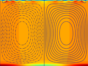
Figure 1. The contour plot of $Ra_\epsilon$ in the $(\bar {T},k)$ plane: (a) $T_M=0$ and (b) $T_M=0.7$.

Figure 2. The critical Rayleigh number $Ra_\epsilon$ computed numerically at $k=10^{-4}$ vs the temperature $\bar {T}$ of the mixing region. Solid lines are obtained by fixing $T_M$ as indicated in the plot. The dashed line illustrates that the minimal Rayleigh number $Ra_\epsilon =64/(1-T_M)^2$ can be achieved at $\bar {T}=(T_M+1)/2$, which agrees well with the numerical solution.

To account for the singular limit of $k\rightarrow 0$, an asymptotic solution is sought. We expand the solution in the region of $z\in [0,1]$ as

(2.22a–c)\begin{equation} \hat{w}=\hat{w}_0(z)+k\hat{w}_1(z)+\dots, \quad \hat{\theta}=\hat{\theta}_0(z)+k\hat{\theta}_1(z)\dots,\quad Ra_\epsilon=Ra_0+kRa_1+\dots, \end{equation}

and the leading-order solution is obtained by using the boundary condition at $z=0$

(2.23a,b)\begin{equation} \hat{w}_0=C_0z^2+C_1z^3,\quad \hat{\theta}_0= - \sqrt{Ra_0}(1-\bar{T})\left(\frac{C_0z^4}{12}+\frac{C_1z^5}{20}+C_2z\right). \end{equation}

Using the conditions in (2.21), we obtain

(2.24a–d)\begin{equation} c_2=C_0,\quad c_0+c_1=0,\quad C_1=0,\quad C_2= - C_0/3\neq0, \end{equation}

and

(2.25)\begin{equation} Ra_0=\frac{16}{(1-\bar{T})(\bar{T}-T_M)}. \end{equation}

One can also solve the problem up to the first-order approximation and obtain the solution for $Ra_1$ (Kerr Reference Kerr2016). However, we will not pursue this since the numerical simulation indicates that $Ra_1>0$. Therefore, the critical Rayleigh number is achieved at $k=0$, in contrast to Currie (Reference Currie1967), which showed that $k=O(1)$ in the Rayleigh–Bénard convection when the top wall is retained. However, if the top wall is moved away, Kerr (Reference Kerr2016) showed that the critical Rayleigh number is also achieved at $k=0$ in the Rayleigh–Bénard convection, which is a common feature between penetrative convection and Rayleigh–Bénard convection. This common feature indicates that large-scale convection can transfer more heat than small-scale motions.

An optimal Rayleigh number $Ra_{opt}$ occurring at $\bar {T}=(1+{T}_M)/2$ can be found from (2.25)

(2.26)\begin{equation} Ra_\epsilon\geqslant Ra_{opt}=\frac{64}{(1-T_M)^2}. \end{equation}

The flow is linearly stable for $Ra_\epsilon < Ra_{opt}$. Note that the numerical solutions in figure 2 are in excellent agreement with the analytical solutions in (2.25) and (2.26) with relative errors smaller than $0.1\,\%$. However, most numerical simulations and the recent optimal steady solutions show that $\bar {T}$ is dependent on the Prandtl number, which also deviates from $(1+T_M)/2$ when $T_M$ is large (e.g. $T_M=0.5,0.7$) (Wang et al. Reference Wang, Zhou, Wan and Sun2019; Ding & Wu Reference Ding and Wu2021). Perhaps, in these previous works, $Ra$ is not high enough or the truncated nonlinear terms are responsible for this deviation.

Under the marginal stability assumption, the piecewise temperature gives the following scaling law of heat transport in penetrative convection as $Ra\rightarrow \infty$:

(2.27)\begin{equation} Ra_\epsilon=2^{ - 3}RaNu^{ - 3}(1-T_M)^3=\frac{64}{(1-T_M)^2}\Rightarrow Nu=\frac{1}{8}(1-T_M)^{5/3}Ra^{1/3}, \end{equation}

where $Nu=(1-T_M)d/(2\epsilon )$. In Ding & Wu (Reference Ding and Wu2021), they assumed that the temperature in the mixing region is linearly dependent on $T_M$ and the bottom wall such that they derived (2.27) (the coefficient was not given). The present work justified their assumption and determined the coefficient $1/8$ using the piecewise background temperature analysis. Currie (Reference Currie1967) derived $Ra_\epsilon =32$ in the classical Rayleigh–Bénard convection using the piecewise background temperature, which is half of the present work ($Ra_\epsilon =64$ when $T_M=0$). It implies that the penetrative convection will show a different heat transport scaling law from the classical Rayleigh–Bénard convection ($Nu\sim 0.315Ra^{1/3}$) at very large $Ra$, although their heat transport is very close for $Ra\leqslant 10^9$ (see Wang et al. Reference Wang, Zhou, Wan and Sun2019; Ding & Wu Reference Ding and Wu2021). It is worth pointing out that the prefactor $1/8$ depends on the choice of the background temperature $\tau$. For instance, in Kerr (Reference Kerr2016), an error function yields $Ra_\epsilon =\sqrt {{\rm \pi} }$ and $Nu\sim 0.330Ra^{1/3}$ can be derived. Therefore, if one chooses a different background temperature profile for penetrative convection, a different prefactor would be expected but the $Ra^{1/3}$ should remain invariant.

3. Conditional lower bound: variational problem

In the previous section, we assumed a given shape for the background profile $\tau$, in this section we solve for the background profile $\tau$ as the numerical solution to a variational problem. In Wen et al. (Reference Wen, Ding, Chini and Kerswell2022), it is shown that a conditional lower bound on the heat transfer in Rayleigh–Bénard convection can be derived based on the marginal stability assumption. It is interesting that the conditional lower bound also exhibits the $1/3$ scaling. In this section, we follow Wen et al. (Reference Wen, Ding, Chini and Kerswell2022) and aim to derive a conditional lower bound on heat transfer in penetrative convection. The neutral stability problem of an unknown $\tau$ is stated as follows:

(3.1)\begin{gather} \boldsymbol{\nabla}\boldsymbol{\cdot}\boldsymbol{u}'=0, \end{gather}

(3.2)\begin{gather}-\boldsymbol{\nabla}p'+\frac{1}{\sqrt{Ra}}\nabla^2\boldsymbol{u}'+2(\tau-T_M)\theta'\boldsymbol{e}_z=\boldsymbol{0}, \end{gather}

(3.3)\begin{gather}\frac{1}{\sqrt{Ra}}\nabla^2\theta'-\frac{{\rm d}\tau}{{\rm d}z}w'=0. \end{gather}

Here, we can also conclude that the scaling law is independent of $Pr$ under the marginal stability assumption.

Using (2.16), we can conclude that

(3.4a,b)\begin{equation} Nu\geqslant Nu_l,\quad Nu_l=\int^1_0\left(\frac{{\rm d}\tau}{{\rm d}z}\right)^2\,{\rm d}z. \end{equation}

It will be interesting to extremise $Nu_l$ such that it delivers a lower bound of heat transport. Therefore, we construct the following Lagrangian:

(3.5)\begin{align} \mathscr{L}&:=\int^1_0\left(\frac{{\rm d}\tau}{{\rm d}z}\right)^2\,{\rm d}z- \left\langle\boldsymbol{u}^{\dagger}\boldsymbol{\cdot}(-\boldsymbol{\nabla}p'+\frac{1}{\sqrt{Ra}}\nabla^2\boldsymbol{u}'+2( \tau-T_M)\theta'\boldsymbol{e}_z)\right\rangle\nonumber\\ &\quad -\left\langle\theta^{\dagger}\left(\frac{1}{\sqrt{Ra}}\nabla^2\theta'-\frac{{\rm d}\tau}{{\rm d}z}w'\right)\right\rangle-\langle p^{\dagger}\boldsymbol{\nabla}\boldsymbol{\cdot}\boldsymbol{u}'\rangle, \end{align}

wherein the marginal stability is imposed as a constraint; $\boldsymbol {u}^{\dagger}$, $\theta ^{\dagger}$ and $p^{\dagger}$ are adjoint variables of $\boldsymbol {u}'$, $\theta '$ and $p'$. It should be stressed that the conditional lower bound is not rigorously derived from the equations of motion. Therefore, the solutions of the full system can either deliver a higher heat flux or a lower heat flux than the conditional lower bound.

Variation of $\mathscr {L}$ gives the following Euler–Lagrange equations:

(3.6)\begin{gather} \delta\mathscr{L}/\delta p^{\dagger}:=\boldsymbol{\nabla}\boldsymbol{\cdot}\boldsymbol{u}'=0, \end{gather}

(3.7)\begin{gather}\delta\mathscr{L}/\delta \boldsymbol{u}^{\dagger}:= - \boldsymbol{\nabla}p'+\frac{1}{\sqrt{Ra}}\nabla^2\boldsymbol{u}'+2(\tau-T_M)\theta'\boldsymbol{e}_z=0, \end{gather}

(3.8)\begin{gather}\delta\mathscr{L}/\delta \theta^{\dagger}:=\frac{1}{\sqrt{Ra}}\nabla^2\theta'-\frac{{\rm d}\tau}{{\rm d}z}w'=0, \end{gather}

(3.9)\begin{gather}\delta\mathscr{L}/\delta p:=\boldsymbol{\nabla}\boldsymbol{\cdot}\boldsymbol{u}^{\dagger} = 0, \end{gather}

(3.10)\begin{gather}\delta\mathscr{L}/\delta \boldsymbol{u}:= - \boldsymbol{\nabla}p^{\dagger} + \frac{1}{\sqrt{Ra}}\nabla^2\boldsymbol{u}^{\dagger} - \frac{{\rm d}\tau}{{\rm d}z} \theta^{\dagger}\boldsymbol{e}_z=0, \end{gather}

(3.11)\begin{gather}\delta\mathscr{L}/\delta \theta:=\frac{1}{\sqrt{Ra}}\nabla^2\theta^{\dagger} + 2(\tau-T_M)w^{\dagger} = 0, \end{gather}

(3.12)\begin{gather}\delta\mathscr{L}/\delta \tau:=2\frac{{\rm d}\tau^2}{{\rm d}z^2}+2\overline{\theta' w^{\dagger}}+\frac{{\rm d}\overline{w'\theta^{\dagger}}}{{\rm d}z}=0. \end{gather}

It is noted that there is a close relationship between the adjoint variables ($\boldsymbol {u}^{\dagger},\theta ^{\dagger},p^{\dagger}$) and the primitive variables ($\boldsymbol {u}',\theta ',p'$) in the Rayleigh–Bénard convection (Wen et al. Reference Wen, Ding, Chini and Kerswell2022), which significantly simplifies the Euler–Lagrange system. However, in the penetrative convection, such a relationship is lost due to the nonlinear constitutive relation (1.1), which complicates the calculation of the Euler–Lagrange equations, i.e. we have to solve a coupled system between the primitive variables and adjoint variables. The Euler–Lagrange equations may admit non-unique solutions when the instability of the base state $(\bar {\boldsymbol {u}},\tau )=(\boldsymbol {0},1-z)$ is subcritical, i.e. solutions can exist when $Ra< Ra_c$ ($Ra_c$ is the critical Rayleigh number for the base state). However, to find a ‘lower’ bound, we only seek solutions which produce the lowest $Nu_l$ for $Ra>Ra_c$. Then, a parametric continuation is used to track the solutions of the Euler–Lagrange equations by continuously increasing $Ra$.

To solve the Euler–Lagrange equations, we expand the variables according to

(3.13a,b)\begin{equation} \begin{pmatrix} u' \\ w' \\ p' \\ \theta' \\ \end{pmatrix} = \begin{pmatrix} \sum_{1}^K u_m(z)\sin(k_mx) \\[6pt] \sum_{1}^K w_m(z)\cos(k_mx) \\[6pt] \sum_{1}^K p_m(z)\cos(k_mx) \\[6pt] \sum_{1}^K \theta_m(z)\cos(k_mx) \\ \end{pmatrix},\quad \begin{pmatrix} u^{\dagger} \\ w^{\dagger} \\ p^{\dagger} \\ \theta^{\dagger} \\ \end{pmatrix} = \begin{pmatrix} \sum_{1}^K u^{\dagger}_m(z)\sin(k_mx) \\[6pt] \sum_{1}^K w^{\dagger}_m(z)\cos(k_mx) \\[6pt] \sum_{1}^K p^{\dagger}_m(z)\cos(k_mx) \\[6pt] \sum_{1}^K \theta^{\dagger}_m(z)\cos(k_mx) \\ \end{pmatrix}. \end{equation}

Here, we assumed that there is a mirror symmetry in the solution (Ding & Wu Reference Ding and Wu2021). Under mirror symmetry, it is easy to prove that $\overline {u'w'}=0$ and $\bar {\boldsymbol {u}}=0$. Although the mirror symmetry may be broken at high $Ra$ (see DNS below), we do not pursue this possibility in the present work because our numerical approach does not find an asymmetric solution of the Euler–Lagrange equations. Hence, the amplitude of the triangle mode satisfies the following equations:

(3.14)\begin{gather} k_mu_m+Dw_m=0, \end{gather}

(3.15)\begin{gather}k_mp_m+\frac{1}{\sqrt{Ra}}(D^2-k^2_m)u_m=0, \end{gather}

(3.16)\begin{gather}-Dp_m+\frac{1}{\sqrt{Ra}}(D^2-k^2_m)w_m+2(\tau-T_M)\theta_m=0, \end{gather}

(3.17)\begin{gather}\frac{1}{\sqrt{Ra}}(D^2-k^2_m)\theta_m-\frac{{\rm d}\tau}{{\rm d}z}w_m=0, \end{gather}

(3.18)\begin{gather}k_mu_m^{\dagger} + Dw_m^{\dagger} = 0, \end{gather}

(3.19)\begin{gather}k_mp_m^{\dagger} + \frac{1}{\sqrt{Ra}}(D^2-k^2_m)u_m^{\dagger} = 0, \end{gather}

(3.20)\begin{gather}-Dp_m^{\dagger} + \frac{1}{\sqrt{Ra}}(D^2-k^2_m)w_m^{\dagger} - \frac{{\rm d}\tau}{{\rm d}z}\theta^{\dagger}_m=0, \end{gather}

(3.21)\begin{gather}\frac{1}{\sqrt{Ra}}(D^2-k^2_m)\theta_m^{\dagger} + 2(\tau-T_M)w^{\dagger}_m=0, \end{gather}

(3.22)\begin{gather}2\frac{{\rm d}\tau^2}{{\rm d}z^2}+\sum^K_1{\theta_m w^{\dagger}_m}+ \frac{1}{2}\sum_1^K\frac{{\rm d}{w_m\theta^{\dagger}_m}}{{\rm d}z}=0. \end{gather}

Here, the notation $D:={\rm d}/{\rm d}z$ is the differential operator with respect to $z$.

The optimal wavenumber $k_m$ for the $m{{\rm th}}$ marginal mode is sought by adding the following equation:

(3.23)\begin{equation} \delta\mathscr{L}/\delta k_m:=\int^1_0u^{\dagger}_m p_m-\frac{2k_m}{\sqrt{Ra}}(u^{\dagger}_m u_m+w^{\dagger}_m w_m+\theta^{\dagger}_m\theta_m)+p^{\dagger}_m u_m\,{\rm d}z=0. \end{equation}

It is crucial to ensure all the modes are marginally stable such that a true lower bound can be yielded. A well-honed technique, i.e. Newton algorithm, has been developed in the study of upper bound problems (Plasting & Kerswell Reference Plasting and Kerswell2003; Ding & Kerswell Reference Ding and Kerswell2020). A complementary method, which uses a time-stepping algorithm, also succeeded in obtaining the upper bound of heat transfer in Rayleigh–Bénard convection (Wen et al. Reference Wen, Goluskin, LeDuc, Chini and Doering2020a). The advantage of the time-stepping algorithm is that it does not require a bifurcation analysis nor a branch continuation technique. Recently, the time-stepping algorithm was utilised to solve the quasilinear problem by O'Connor et al. (Reference O'Connor, Lecoanet and Anders2021) and then the lower bound on heat transport in Rayleigh–Bénard convection (Wen et al. Reference Wen, Ding, Chini and Kerswell2022). We should point out that, unlike the upper bound problem, the time-stepping algorithm does not guarantee the global optimal solution in either the quasilinear problem or the conditional lower bound problem. Also, it requires quite a long time to reach to a steady state and the time-stepping algorithm cannot be used to find an unstable ‘steady’ state. Indeed, we have known that the stability of the trivial state $(\bar {\boldsymbol {u}},\tau )=(\boldsymbol {0},1-z)$ is subcritical when $T_M\geqslant 0.4$ and $Pr=1$ (Ding & Wu Reference Ding and Wu2021). Therefore, the present work chooses the Newton algorithm and branch continuation to track the solutions for the conditional lower bound problem and the quasilinear problem in § 4. To check if there is a new unstable mode emerging as $Ra$ increases, we have to solve (2.13)–(2.15) and examine if there is a positive eigenvalue $\lambda$, which is introduced into the problem by the normal mode analysis: $(\boldsymbol {u}',\theta ')=(\hat {\boldsymbol {u}},\hat {\theta })\exp ({\rm i}kx+\lambda t)$.

Figure 3 shows the dispersive relation of a marginally stable state at $Ra=10^9$. For $T_M=0$, we have detected $7$ marginally stable modes, while there is only $1$ marginally stable mode for $T_M=0.7$. Another interesting feature is that the eigenvalue $\lambda$ is real for all wavenumbers $k$ when $T_M=0$, while it is complex for $40< k<90$ when $T_M=0.7$ (in Rayleigh–Bénard convection, all the leading eigenvalues are real O'Connor et al. Reference O'Connor, Lecoanet and Anders2021; Wen et al. Reference Wen, Ding, Chini and Kerswell2022). Although the mode with a complex eigenvalue is linearly stable, it might be important when the fully nonlinear system is considered. The bifurcation diagram of the critical modes is illustrated in figure 4. For small $T_M$ ($T_M\leqslant 0.1$), the penetrative convection is very similar to the Rayleigh–Bénard convection, and the bifurcation diagram exhibits a hierarchical structure (new unstable modes emerge as $Ra$ increases). When $T_M>0.1$, only a single critical mode is detected using our algorithm, e.g. $T_M=0.3$, $0.7$. This demonstrates that the thickness of the stable layer plays an important role in selecting the marginal modes.

Figure 3. The dispersive relation of a marginally stable state obtained using the variational problem at $Ra=10^9$.

Figure 4. The bifurcation diagram of the wavenumber $k_m$, (a–d) $T_M=0,0.1,0.3,0.7$. Each line stands for the wavenumber $k_m$ of the $m{{\rm th}}$ mode vs the Rayleigh number $Ra$. In (a,b), large wavenumber modes appear in pairs (adjacent solid and dashed lines). In (c,d), only a single critical mode is detected.

To illustrate the critical modes at different values of $T_M$, two typical cases of $T_M=0$ and $T_M=0.3$ are plotted in figures 5 and 6. For $T_M=0$, there are seven marginal modes: a central mode with six wall modes (the wall mode either concentrates near the top wall or the bottom wall, and they usually appear in pairs). The wavenumber of the central mode is of order $O(1)$, which seems to persist as $Ra\rightarrow \infty$, and the wavenumber of other modes scales as $Ra^{1/3}$ (see figure 4). Equation (2.27) shows that the thickness of a marginally stable boundary layer $\epsilon$ scales as $Ra^{-1/3}$. Therefore, if the convection cell is confined within the boundary layer, then its size is proportional to the boundary layer thickness and we can immediately obtain $k=2{\rm \pi} /\epsilon \sim Ra^{1/3}$. Like the long-wave analytical solution in § 2.2, the central mode, which occupies the whole domain, represents the large-scale motion in the system. However, for $T_M=0.3$, there is only a single marginal mode which always concentrates near the bottom wall (the corresponding wavenumber also scales as $Ra^{1/3}$). Such an interesting feature indicates that convection is confined within the boundary layer near the bottom wall and the outside fluid is stationary. Figure 7 demonstrates that the background temperature profile does have two boundary layers when $T_M\lesssim 0.1$ and it only has a single boundary layer when $T_M>0.1$. Nevertheless, we observe that the background temperature profile is not physical: the heat flux is not conserved – the heat flux at the bottom wall is not equal to that at the top wall. This non-physical feature is caused by the non-physical driving force in (3.22). Therefore, we can conclude that the variational problem delivers a non-physical bound for the penetrative convection, which, however, delivers a physically plausible solution in the classical Rayleigh–Bénard convection (Wen et al. Reference Wen, Ding, Chini and Kerswell2022). If the solution of the full system satisfies the marginal stability assumption, it should deliver a higher heat flux than the present conditional lower bound. If heat flux in the full system is lower than the present conditional lower bound, the corresponding mean field should violate the marginal stability assumption, i.e. the averaged field is not marginally stable.

Figure 5. The eigenvectors of the marginally stable state obtained from the variational problem: $T_M=0$ and $Ra=10^9$. In (c,d), zoom-in insets are shown.

Figure 6. The eigenvectors of the marginally stable state obtained from the variational problem at different Rayleigh numbers and $T_M=0.3$.

Figure 7. The marginally stable temperature profile obtained from the variational problem at $Ra=10^9$.

4. Quasilinear problem

In § 3, the background temperature derived from the variational problem is non-physical because of the non-physical driving force. Now, we examine the marginal stability assumption of $\tau$ that is yielded from the quasilinear problem, i.e. the background temperature field is driven by the perturbation field (see (2.9))

(4.1)\begin{equation} \frac{{\rm d}^2\tau}{{\rm d} z^2}=\frac{\sqrt{Ra}}{2}\sum_1^K\frac{{\rm d} (w_m\theta_m)}{{\rm d}z}. \end{equation}

Note that the Prandtl number $Pr$ can also be scaled out from (4.1) by introducing $\theta '/\sqrt {Pr}\rightarrow \theta '$. The global heat transfer is conserved when the background temperature field is driven by the physical perturbations. Using (4.1), we can expect that if there is a boundary layer near the bottom wall, there should be a complementary boundary layer near the top wall. Using the Newton algorithm, it is more tedious to find the solution of (3.14)–(3.21) and (4.1) than the variational problem in § 3, because there is no equation for the wavenumber $k_m$ in the quasilinear problem. In O'Connor et al. (Reference O'Connor, Lecoanet and Anders2021), both harmonic and sub-harmonic waves were included in their quasilinear problem, i.e. $k_m=mk_c/2$ ($m\in \mathbb {N}^+$ and $k_c$ is the critical wavenumber of primary instability). It indicates that we should consider an infinitely long domain to allow those harmonic and sub-harmonic waves. In Wen et al. (Reference Wen, Ding, Chini and Kerswell2022), a finite domain of size $L=2{\rm \pi} /k_c$ was considered and $k_m=mk_c$ ($m\in \mathbb {N}^+$). Comparison between O'Connor et al. (Reference O'Connor, Lecoanet and Anders2021) and Wen et al. (Reference Wen, Ding, Chini and Kerswell2022) indicates that the domain size's effect is negligible. Hence, we follow Wen et al. (Reference Wen, Ding, Chini and Kerswell2022) and fix the domain size in the present work, which also allows us to perform DNS with initial conditions seeded by the quasilinear problem.

The bifurcation diagram of $k_m$ is illustrated in figure 8, indicating that the quasilinear problem undergoes a hierarchical bifurcation as $Ra$ increases for all $T_M$, which is an obviously different feature from the lower bound problem. The central mode $m=1$ is always critical for all $T_M$ in the quasilinear problem. The largest two wavenumbers exhibit a $Ra^{1/3}$ scaling, as demonstrated in figure 8, which implies that there are two boundary layers in the system. Thicknesses of the two boundary layers are proportional to $Ra^{-1/3}$ and convection cells should be confined within them. Figure 9 demonstrates that the two modes $m=23$, $25$ are concentrated in the near-wall regions, which are due to the instability of the boundary layers. Figure 9 also indicates that larger-scale convection contains more kinetic energy.

Figure 8. The bifurcation diagram of the wavenumber $k_m$ of the quasilinear problem, (a–d) $T_M=0,0.1,0.3,0.7$.

Figure 9. The eigenvectors of the marginally stable state obtained from the quasilinear problem: $T_M=0$ and $Ra=10^9$.

Figure 10 depicts the profiles of the background temperature of the quasilinear problem at $Ra=10^9$. It demonstrates that the boundary layers become thicker and the asymmetry of $\tau$ becomes more conspicuous as $T_M$ increases (the top boundary layer is thicker than the bottom boundary layer). The mean temperature in the bulk region increases but the mean temperature is below $(T_M+1)/2$. It may be caused by the constraint of the top wall or the relatively low Rayleigh numbers ($Ra\ll \infty$). A similar feature to the classical Rayleigh–Bénard convection is that there are also two dips in the profile of background temperature. However, as $T_M$ increases, the protruding part of the lower ‘dip’ becomes smaller, while it remains significant in the top ‘dip’. The ‘dip’ structure, however, is not significant in the optimal horizontal-averaged temperature profiles. In addition, figure 10 indicates that the quasilinear problem predicts a thinner boundary layer than the optimal steady solution by Ding & Wu (Reference Ding and Wu2021), and it seems that the optimal steady solution yields a mean temperature profile that is more consistent with the Malkus (Reference Malkus1954) hypothesis. Unlike the penetrative convection, the ‘dip’ structures are significant in both the steady optimal solutions (Sondak et al. Reference Sondak, Smith and Waleffe2015) and the quasilinear problem (O'Connor et al. Reference O'Connor, Lecoanet and Anders2021) of the classical Rayleigh–Bénard convection. The predicted mean averaged temperature in the bulk region is a bit lower than the optimal horizontal-averaged temperature due to the consequence of thinner boundary layers. It also indicates that the quasilinear problem predicts a higher heat flux than the optimal steady solution.

Figure 10. The marginally stable temperature profiles (lines) obtained from the quasilinear problem at $Ra=10^9$. Symbols are the optimal horizontal-averaged temperature obtained from Ding & Wu (Reference Ding and Wu2021) at $Ra=10^9$, $Pr=1$.

Furthermore, we plot the Nusselt number predicted by the quasilinear approach and the conditional lower bound in figure 11, and the Nusselt number is rescaled by $(1-T_M)^{-5/3}$. It is interesting that the quasilinear approach shows that $Nu\sim 0.17(1-T_M)^{5/3}Ra^{1/3}$ when $T_M\geqslant 0.3$ (lines are almost overlapping). But for small $T_M$, the quasilinear approach shows that heat transport is slightly lower than $0.17(1-T_M)^{5/3}Ra^{1/3}$, which, perhaps, is because the Rayleigh number is not large enough (however, they are very close to $(1/8)(1-T_M)^{5/3}Ra^{1/3}$). An interesting feature is that the line can be multi-valued when the instability of the base state $(\bar {\boldsymbol {u}},\tau )=(\boldsymbol {0},1-z)$ is subcritical (see the solid lines for $T_M=0.5$, $0.7$ in figure 11). This indicates that the background temperature field is non-unique, although the lower branch is linearly unstable (Ding & Wu Reference Ding and Wu2021). Note that the subcritical instability nature of penetrative convection indicates that the retained nonlinear term $\partial _z\overline {w'\theta '}$ destabilises the base state $(\bar {\boldsymbol {u}},\tau )=(\boldsymbol {0},1-z)$, thus contradicting Malkus's assumption. At high $Ra$, our algorithm did not find a double-branch solution but this does not mean the solution of the quasilinear problem is unique. The lower bound roughly follows $(1-T_M)^{5/3}Ra^{1/3}$ when $T_M\leqslant 0.3$, and it deviates from $(1-T_M)^{5/3}Ra^{1/3}$ when $T_M$ is large, which perhaps is also because of the relatively low $Ra$. Both the quasilinear problem and the lower bound indicate that $Nu\sim Ra^{1/3}$.

Figure 11. The Nusselt number $Nu$ vs the Rayleigh number $Ra$; ‘QL’ stands for quasilinear problem (solid lines) and ‘VS’ is for the variational lower bound problem (dashed lines).

5. Direct numerical simulations

In previous sections, different choices of the background field $\tau$ were examined and the ensuing turbulent heat transport under the marginal stability assumption was examined. Now we investigate the heat transport and flow fields using DNS. To check the influence of the truncated nonlinear terms in the quasilinear problem, DNS are performed by initialising simulations with the quasilinear states. Aiming at understanding how mirror symmetry influences the turbulent state, two different sets of simulations were performed: (i) with a mirror symmetry (ii) without a mirror symmetry. Here, we only consider a two-dimensional study. If there are two different statistical states emerging from the two sets of numerical simulations, this indicates that the turbulent state is degenerate in penetrative convection. The spatial discretisation was accomplished using a Fourier-spectral method. The axial direction was discretised with a Fourier transform (Frigo & Johnson Reference Frigo and Johnson2005) and the 2/3 dealiasing rule was implemented. A finite difference method with non-uniform grid clustering near the walls (Chebyshev points) was used in the wall-normal direction. The time discretisation was accomplished with a second-order Adams–Bashforth–Crank–Nicolson method. Details of the numerical method can be found in Willis (Reference Willis2017) and Ding & Wu (Reference Ding and Wu2021).

To illustrate the nonlinear evolution of the quasilinear state, we consider two cases of $T_M=0$, $0.7$. The Nusselt number is monitored during the numerical simulation, as shown in figures 12 and 14, which demonstrates that the quasilinear steady state is nonlinearly unstable. It also indicates that the Nusselt numbers of the symmetric and asymmetric cases are identical and the flow becomes steady when the Rayleigh number is low (e.g. $Ra=10^7$). However, as $Ra$ increases to $10^8$, we observe that the time series of $Nu(t)$ start to deviate from each other as $t$ increases and both cases are chaotic. This suggests that the system can allow different chaotic solutions, i.e. the ‘turbulent’ state can be degenerate in penetrative convection. It also implies that the background temperature field can be non-unique at high $Ra$ since we can obtain different averaged fields using the simulation data. Figures 12 and 14 also demonstrate that spontaneous symmetry breaking occurs at high Rayleigh number in the system. To illustrate the spontaneous symmetry breaking, we plot the flow field and thermal field in figures 13 and 15. For $T_M=0$, only two large convection cells are observed in both the symmetric simulation and asymmetric simulation. However, in the asymmetric simulation, the hot plume near the bottom wall and the cold plume near the top wall start to oscillate when symmetry breaks, causing a mean ‘wind’ flow in the system. The mean ‘wind’ flow is time periodic as indicated by the vortex incline angle. As demonstrated in figure 12, the oscillating asymmetric flow generally transfers less heat than the symmetric flow. However, for $T_M=0.7$, we observe that the asymmetric flow can transfer more heat than the symmetric flow, as demonstrated in figure 14, in contrast to the case of $T_M=0$. Unlike the case of $T_M=0$, we observe that the initial field develops into a two-layer structure which undergoes the spontaneous symmetry breaking at $t\approx 160$. The two-layer structure is unstable, which evolves into a symmetric four-convection-cell structure or an asymmetric two-convection-cell structure as demonstrated in figure 15. Note that the width of the symmetric four-convection-cell structure is approximately half of the asymmetric two-convection-cell, indicating that large-scale motion can transfer more heat.

Figure 12. The evolution of Nusselt number with time $t$ at $Pr=1$, $T_M=0$. The solid (dashed) lines represent simulation results with (without) mirror symmetry.

Figure 13. The instantaneous flow and thermal fields computed at $Pr=1$, $T_M=0$ and $Ra=10^9$.

Figure 14. The evolution of Nusselt number with time $t$ at $Pr=1$, $T_M=0.7$. The dashed (solid) lines represent simulation results with (without) mirror symmetry.

Figure 15. The instantaneous flow and thermal fields computed at $Pr=1$, $T_M=0.7$ and $Ra=10^{10}$.

The long-time average of Nusselt number $Nu$ is rescaled by factor $(1-T_M)^{-5/3}Ra^{-1/3}$ ($Nu$ is averaged within $t\in [1000,2000]$) and plotted against $Ra$ as shown in figure 16. For $T_M=0.5$, $0.7$, we observe that heat transport via optimal steady solution (Ding & Wu Reference Ding and Wu2021) follows $(1-T_M)^{5/3}Ra^{1/3}$ asymptotically. And the optimal steady solution transfers more heat than the two-dimensional ‘turbulent’ states (both symmetric and asymmetric simulations deliver lower $Nu$ than the optimal steady solution). The heat transport by two-dimensional ‘turbulent’ states and the optimal steady state is bounded by the quasilinear solution and the lower bound. However, for $T_M=0$, 0.1, 0.3, heat transport by the two-dimensional ‘turbulent’ states and the optimal steady state is lower than the lower bound when the Rayleigh number is large. This indicates that the averaged thermal field of the two-dimensional ‘turbulent’ states is not marginally stable. In this sense, it contradicts the hypothesis of Malkus (Reference Malkus1956). However, figure 16 implies that the background field is over-stabilised by the nonlinear terms at high $Ra$ and the global heat transfer is consequently reduced, which agrees well with Malkus's assumption. It should be also stressed that the heat transfer computed using the full system is less than the quasilinear problem, similar to the findings by Wen et al. (Reference Wen, Ding, Chini and Kerswell2022) in Rayleigh–Bénard convection. Although many previous works claimed that penetrative convection is almost identical to the Rayleigh–Bénard convection when $T_M=0$, it is questionable whether the $Nu\sim Ra^{1/2}$ scaling can be observed in penetrative convection as $Ra\rightarrow \infty$.

Figure 16. The Nusselt number $Nu$ vs the Rayleigh number $Ra$. ‘OP’ stands for optimal solution in Ding & Wu (Reference Ding and Wu2021). ‘DNSS’ (‘DNSA’) is for the direct numerical simulation with (without) mirror symmetry. Solid lines are quasilinear approximation and dashed lines are the variational lower bound for various values of $T_M$: blue lines for $T_M=0$; red lines for $T_M=0.1$; green lines for $T_M=0.3$; magenta lines for $T_M=0.5$; cyan lines for $T_M=0.7$.