


Introduction
Passive or active observations of ice masses in the microwave domain may provide important parameters, if the dielectric behaviour of the snow is well known, which is not the case. For example, satellite-radar altimeters allow the mapping of ice-surface topography (Reference Zwally, Bindschadler, Brenner, Martin and ThomasZwally and others, 1982; Reference Remy, Mazzega, Houry, Brossier and MinsterRemy and others, 1989) if the signal is not affected significantly by volume-scattering within the snowpack.
Passive microwave radiometry, which is sensitive to the grain-size profile in the upper few meters below the snow surface (Reference ZwallyZwally, 1977), may provide a measurement of accumulation rate (Reference Rotman, Fisher and StaelinRotman and others, 1982). However, Reference Remy and MinsterRemy and Minster (1991) suggested that the polarization of microwave emission is affected by surface micro-roughness of the ice sheets. Matzler (1987) also suggested that internal layering plays an important role in the radiometric signal.
The behaviour of microwaves in the snowpack is not understood well because of the complexity of this natural medium (Reference Rott and PampaloniRott, 1989). The signal can be affected by surface, sub-surface and volume back-scatter, or by surface roughness on various scales. Parameters such as temperature, grain-size, statistics of the surface roughness and snow layering must be considered. Theoretical studies are, therefore, complex and inconclusive. Empirical studies of altimetric return power or radiometer emissivity are also limited. Reference Remy, Brossier and MinsterRemy and others (1990) showed that the intensity of the Seasat altimeter return power over Antarctica varies in strong correlation with the intensity of model katabatic winds. This can be explained by surface-scattering, which is related to surface micro-roughness (Reference Fung and EomFung and Eom, 1982) created by the surface wind or by volume-scattering, which is proportional to the snow grain-size, also affected potentially by wind speed.
The nature of microwave back-scatter coefficients on snow is examined here empirically using scatterometer data. (The back-scatter coefficient is the ratio of the return power over the incidence power, generally expressed in decibels.) The advantage of the scatterometer radar instrument is that it provides observations for several incidence and azimuth angles (see Fig. 1 for definition), and for both horizontal and vertical polarizations of the signal. For the Seasat scatterometer, each satellite path provides 15 values at two different incidence angles for both polarizations. Contrary to other instruments (altimeter or radiometer) which provide single observations, scatterometer readings contain about 60 different observations per satellite path (i.e. 15 observations by each of two antennas at two polarizations). This large data set may better describe the different scattering processes. Further theoretical studies suggest that at small incidence angles, the back-scatter coefficient will be sensitive to surface-scattering, whereas at greater incidence angles, volume-scattering will be dominant (Reference Fung and EomFung and Eom, 1982). Reference Swift, Hayes, Herd, Jones and DelnoreSwift and others (1985) reached the same conclusion from studies of airborne microwave measurements above the Greenland ice sheet. Yet, to our knowledge, no previous study of the Seasat scatterometer data above continental ice sheets has been published.

Fig. 1. Geometry of the observations by the Seasat A scatterometer (adapted from Reference Johnson, Williams, Bracalente, Beck and GranthamJohnson and others, 1980). The lines in the figure represent the lines of constant Doppler effect on the echo, which is used to separate the data into cells.
The physical principles of the Seasat scatterometer are introduced in the first section of this paper. The variations of the back-scatter coefficient as a function of different parameters are then analyzed empirically using data from various areas of the Antarctic ice sheet. The direction and intensity of the surface winds are calculated in the third section. The results of simple theoretical models of surface- and volume-scattering are compared with the observations in the last section.
The Seasat-a Satellite Scatterometer
The SASS (Seasat-A satellite scatterometer) was designed to measure ocean-surface wind speed and direction. It has been described in detail by Reference Johnson, Williams, Bracalente, Beck and GranthamJohnson and others (1980) and Reference Bracalente, Buggs, Grantham and SweetBracalente and others (1980). It operates at a microwave frequency of 14.6 GHz with four beam antennae. Two antennae view each side of the satellite, each one at an angle of 45 ° relative to the satellite track (forward and backward) (Fig. 1). Each of these antennae is composed of 15 “cells” (corresponding to different angles varying from 0 to 64 °) giving measurements of the back-scatter coefficient. Three cells operate at small incidence angles (0–8 °) and 12 at large incidence angles (25–64 °). One cell is represented by an incidence angle varying by about 3 °, leading to a resolution of 50 km in the antenna beam direction and 16 km perpendicular to it. Measurements are taken every 1.89 s, the antenna switching cycle being completed in 7.56 s. The back-scatter coefficient in each cell is derived by averaging 15 individual measurements.
The use of independent measurements from two antennae with orthogonal azimuthal viewing angles for each cell was required to deduce both wind speed and direction above the ocean. Indeed, for a given incidence angle, the radar back-scatter is observed to vary with azimuth angle following a bi-sinusoidal curve (Fig. 2). The same figure also indicates variations of the back-scatter coefficient with incidence. In the following study, our results are compared with those shown in Figure 2. In the case of the ocean, models including a statistical description of sea-surface height and slope distributions are used to explain the observed signal. An empirical approach is used here in the case of the ice sheets.

Fig. 2. Typical variations of the back-scatter coefficient σ0ο above the ocean as a function of incidence angle θ, of polarization (VV or HH), of wind speed and azimuth relative to the wind (adapted from Reference StewartStewart, 1985). This figure will be used as a reference to ice-sheet data.
Methodology
The surface roughness of the ocean and ice sheets have very different statistical characteristics. For the ocean, the temporal evolution of surface sea state is very rapid and the spatial signal has a large wavelength (the synoptic scale of the atmosphere). This is because the ocean and surface gravity waves respond quickly to atmospheric winds. For the Antarctic ice sheet, the back-scatter is expected to be “quasi-permanent”, as all parameters (temperature, grain-size, surface roughness) may remain constant on the decadal time-scale (personal communication from D.H. Bromwich). In addition, even though the intensity of the wind varies strongly with time, the geography of its pattern is stationary. Indeed, the prevailing winds are katabatic, their flowlines being mostly controlled by the ice-sheet topography and by the Earth’s rotation (Fig. 3). The Seasat altimeter back-scatter coefficient averaged over time varies on the distance scale of 100 km (Fig. 4). This provides an a priori estimate of the length scale of variations for the scatterometer signal, at nadir, because it operates at the same frequency as the altimeter.

Fig. 3. Isolines of the topographic height of the Antarctic ice sheet (from Reference Drewry and DrewryDrewry, 1983) and ßowlines of the model katabatic winds (from Reference ParishParish, 1982). The four selected regions are indicated.

Fig. 4. Geophysical variations of the back-scatter coefficient measured by the Seasat altimeter (adapted from Reference Remy, Brossier and MinsterRemy and others, 1990).
Four regions characterized by the following criteria are analyzed: a sufficiently large surface to contain data at many azimuth and incidence angles and a sufficiently small surface for the “forcing” parameters to be spatially homogeneous (in order to help separate their effects). The latter include two effects: strength of the wind for the potential effects on surface echo and grain-size for the effects on volume echo. The former depends on the lateral convergence and divergence of the flow, and on the terrain slope (Reference Parish and BromwichParish and Bromwich, 1991). It is, therefore, to a first order, related inversely to the altitude and to the distance between katabatic-wind flowlines in Figure 3, and may be deduced from Reference Parish and BromwichParish and Bromwich (1991). The latter effect is affected strongly by temperature (or equivalently, by altitude to a first order), as low temperatures induce large grain-sizes.
This results in the regions shown in Figure 3: region A is characterized by a light wind and high altitude (2900 m), region Β by a very strong wind and relatively low altitude (1800 m), region C by a strong wind and high altitude (2800 m) and region D by a strong wind and low altitude (2000 m).
In this study, we analyze one 17 d cycle of the Seasat orbit, using between 1000 and 2000 individual scatterometer measurements for each region.
Empirical Study
The back-scatter coefficient varies from −20 to 10 dB in the whole data set. The correlations of the back-scatter coefficient with various parameters and the behavior of the data in the four regions are analyzed successively as a function of incidence, azimuth angle and polarization. In what follows, only data with signal to noise (S/N) values larger than 10 dB, as measured by the instrument, are considered. Because little is known a priori about the signal, the main features are first identified and then discussed.
Correlation with Different Parameters
In Figure 5, in order to have a more complete sampling, we use the whole data set to study correlations of scatterometer data with the altimeter back-scatter coefficient, with altitude and with radiometric data at 37 GHz measured by the Nimbus 7 SMMR (Scanning Microwave Radiometer) at 50 ° incidence angle (vertical and horizontal emissivities ev and eh , respectively, and the difference between both polarizations). The results are considered significant when the correlation coefficient exceeds 0.4, which means that more than 16% of the signal can be explained by the correlation. They are as follows:
-
(i) The scatterometer back-scatter coefficient is correlated strongly with that of the altimeter at low incidence. As already observed for altimetry (Reference Remy and MinsterRemy and Minster, 1991), the signal at low incidence angle is correlated strongly with the polarization of the emissivity. This effect, due to the presence of micro-roughness, disappears at higher incidences.
-
(ii) We do not observe any correlation with altitude. On the other hand, a significant correlation exists between the back-scatter coefficient and horizontal and vertical emissivity for “large” incidence angles.

Fig. 5. Correlation of the scatterometer back-scatter coefficient with the Seasat altimeter σ0, with altitude, with emissivities at 37 GHz and 50 ° incidence angle deduced from the Nimbus 7 SMMR data and with polarization of the latter signal.
The correlation with emissivity, a parameter connected with snow grain-size, would suggest the possible effect of a volume echo; however, this is in contradiction to the absence of correlation with altitude (or with temperature; snow grain-size, being temperature dependent, is related to altitude). In addition, the correlation with emissivity could be explained by surface roughness for horizontal polarization, but not for vertical polarization (Reference Tsang and NewtonTsang and Newton, 1982). Because of this, further analyses were performed in the four regions.
Polarization Versus Incidence Angle
Polarization of the back-scatter coefficient is shown as a function of incidence angle (Fig. 1) for the four regions (Fig. 6). Note that because the surface slope is less than 0.2 °, even for region B, its effect on the position of the pixel is much smaller than the size of the illuminated domains. As a consequence, the incidence angle as measured on board the satellite does not need to be corrected for surface-slope effects. The polarization is small and varies from −2 to 3 dB. It is erratic at low and very large incidence angles. Otherwise, the signal for vertical polarization is slightly larger than for horizontal polarization and the difference tends to increase with incidence angle.

Fig. 6. Polarization of the scatterometer signal (in dB) as a function of incidence angle. The dotted line represents the reference curve of region A, fitted by averaging the values for each cell.
Back-Scatter Coefficient Versus Incidence Angle
The Variations of the back-scatter coefficient versus incidence angle for the four regions are shown in Figure 7. Data for the two polarizations are used simultaneously. The signal is strongest in the vertical and decreases with incidence angle towards a steady value. However, for a given incidence angle, the back-scatter signal fluctuates by as much as 10 dB. Regions A, C and D have similar characteristics, whereas, in region B, the signal is lower by 4 dB at low incidence angles and higher by the same amount at large incidence angles. Only surface-scattering can explain this decrease with respect to incidence angle, as discussed later.

Fig. 7. Back-scatter coefficient as a function of incidence angle (in degrees) for the four regions. The continuous lines join the mean values for each cell. The dotted line is the line for region A, used as a reference.
Back-Scatter Coefficient Versus Azimuth Angle
The variations of the back-scatter signal minus the average back-scatter intensity for each cell (called the residual back-scatter coefficient) versus azimuth angle are shown in Figure 8. Although it is not complete, the distribution of azimuth is sufficient for observing that the residual back-scatter coefficient varies from −5 to 5 dB, with well-defined minima and maxima. As in the case of the ocean, a bi-sinusoidal curve is shown in Figure 8. It is specified by
where σ is the back-scatter coefficient and σmoy is the back-scatter coefficient averaged for each cell. ϕ is the azimuth of observation and ϕ0 that of the minimum. The coefficients α and ϕ0 were estimated by least-squares regression. Although the azimuth sample is well distributed for the whole data set, this is not the case for each cell; thus σmoy is re-estimated after a first iteration on α and ϕ0 The final results are given in Table 1.

Fig. 8. Residual back-scatter coefficient (in dB) as a function of azimuth (in degrees) for the four regions. The residues are calculated for each cell by subtracting the mean value. The model curves corresponding to Equation (1), with the parameters of Table 1, are shown for comparison. The arrows indicate the azimuth of the model katabatic winds of Reference ParishParish (1982).
Table 1. Variation of the residual back-scatter coefficient versus azimuth angle, a and ϕ0 are coefficients from Equation (1) adjusted by least-squares regression. ϕw is the azimuth of katabatic winds deduced from Figure 4.![]() is the reduced X2
of the fit between Equation (1) and the data normalized to data noise. The regions are characterized according to wind intenúty and altitude
is the reduced X2
of the fit between Equation (1) and the data normalized to data noise. The regions are characterized according to wind intenúty and altitude

The fit to the model is estimated by a normalized, reduced ![]() defined as
defined as

In this calculation, Ν is the number of data, σmodel is calculated from Equation (1) for the azimuth value ϕn of the datum. The normalization corresponds to S/Ν = 10 dB. In principle, X2 should be close to 1 if the model fits the data. It is generally on the order of 4, which is acceptable, but larger for region D. Much spreading for this region is shown in Figure 8.
The parameter α is largest for region B, which has the strongest wind. It induces a signal of 5 dB amplitude, which is indeed close to observations. ϕ0 the azimuth angle for maximum amplitude, is always at about 90 ° from the wind direction, as determined independently from the katabatic-wind flowlines (Reference ParishParish, 1982; Reference Parish and BromwichParish and Bromwich, 1991; Fig. 3).
Finally, region Β data were analyzed by separating them according to polarization and incidence angle (we used three sets of four cells from numbers 1–4, 5–8 and 9–12). In each case, the variation with azimuth was similar.
Discussion
As a whole, the signal over ice is very similar to that above the ocean (Reference StewartStewart, 1985; Fig. 2). The strong decrease of the back-scatter coefficient at low incidence suggests a surface effect, because the variations in the case of a volume echo would be small. The variations in residual back-scatter with azimuth at all incidence angles again suggests a surface-roughness effect. It would be necessary that the reflecting features be orientated in the wind direction for the back-scatter to be minimum in that direction. This is the case for sastrugi. They are streamlined ridges formed on the snow surface by the wind and are orientated in the wind direction (Reference Parish and BromwichParish and Bromwich, 1987; Reference Bromwich, Parish and ZormanBromwich and others, 1990).
Region Β differs from the other three regions. It has a lower signal at low incidence angles, a stronger signal at strong incidence angles and a larger sensitivity to azimuth. All three features are coherent with a surface-roughness effect, as Β is the region of strongest winds.
Finally, a surface effect could explain the large variations of the signal at low incidence angle (Fig. 7). These variations could be due to measurement effects, such as propagation of the radar wave in the atmosphere, or to actual signal variations. It would be surprising if atmospheric effects, which can indeed reach 10 dB, only affect measurements at low incidence angles. On the other hand, Reference Remy, Brossier and MinsterRemy and others (1990) showed that surface undulations with a 20 km distance scale could induce variations in the altimeter returned power of about 10 dB, which is of the same order as observed here.
However, polarization is weak, whereas the surface-roughness effect should have an influence. In addition, we have already mentioned that surface roughness should not affect emissivity at the vertical polarization. In any case, it is desirable to analyze the potential effects of the surface and sub-surface snow state more quantitatively. This is the object of the following section.
Theoretical Study
In order to analyze more quantitatively whether the observed signals can be explained by the known ranges of the critical parameters, a simple discussion of two models for volume and surface echos is presented.
Volume Echo
Theoretical models of volume-scattering by snow are based on Rayleigh’s radiative-transfer method. The volume diffusion per surface unit is written (Reference RottRott, 1984, Reference Rott, Domik, Mätzler, Miller and Lenhart1985):

where lr
and lz
are correlation lengths of snow, corresponding to the average of the grain-size (Reference Valiese and KongValiese and Kong, 1981), which we will take as spherical (lr = lz), ε1 is the permittivity for snow. Its value depends on snow density as ε1 = 1 + 1.7ρ + 0.7ρ2. As ρ varies from 0.35 to 0.45 Mgm−3, ε1 varies from 1.68 to 1.91. ε1 is equal to 1. δk is the permittivity fluctuation of snow and is taken at 0.24 (Reference Valiese and KongValiese and Kong, 1981). t is the transmittivity; in this case, it has a value of 1. θ is the incidence angle. θt is the angle of transmission, related to θ by Snell’s law of refraction: sin θt = ![]() is the wave number in the medium, where k1
= 2π/λ, λ is the radar wavelength, that is 2.3 cm for Seasat. Ka
is the volume-absorption coefficient, which depends on the dielectric constant and varies between 0.05 and 0.2 according to Ulaby and Styles (1980) and Reference MätzlerMätzler (1987). Here, we take the value Ka
= 0.2 because values below this are too low to explain the radiometric observations (Reference Rott and PampaloniRott, 1989).
is the wave number in the medium, where k1
= 2π/λ, λ is the radar wavelength, that is 2.3 cm for Seasat. Ka
is the volume-absorption coefficient, which depends on the dielectric constant and varies between 0.05 and 0.2 according to Ulaby and Styles (1980) and Reference MätzlerMätzler (1987). Here, we take the value Ka
= 0.2 because values below this are too low to explain the radiometric observations (Reference Rott and PampaloniRott, 1989).
The first bracket within Equation (3) is independent of incidence angle and only has an effect on the signal intensity. It varies with the absorption coefficient or with permittivity fluctuations. However, it is most sensitive to grain-size as it depends on the cube of 1r . The second term is a function of the incidence angle. The curvature of back-scatter coefficient versus incidence angle varies with snow-grain radius and permittivity.
Back-scatter values, changing from −37 to –18 dB for lr values varying from 0.3 to 1 mm (Reference GowGow, 1960), are shown in Figure 9. At large incidence angles, the theoretical intensity is comparable to the experimental data of Figure 8. However, the fit is not good at low incidence angles. Thus, volume diffusion alone does not seem to explain the observations. Of course, at this stage, the effects of multiple scattering or of complex layering cannot be excluded.

Fig. 9. Variations of the back-scatter coefficient as a function of incidence angle in the case of volume-scattering. The curves are shown for various grain-sizes lr from 0.3 to 1 mm.
Surface Echo
When an incident wave intersects a smooth surface, the reflected signal is principally a coherent or specular component, which is directional. The rougher the surface, the higher the diffuse component and the less coherent the echo. The surface roughness will be characterized either by its correlation length L and its root-mean-square (r.m.s.) height σL, or instead by its r.m.s. surface slope, m Roughness is to be compared with the wavelength of the radar signal λ. The echo model will depend on the value of k 1 σ L = (2π/λ)σ L. The effect of a rough surface on the scattered power is analyzed in different cases, as in Reference FungFung (1984). We consider only the extreme cases, the intermediate one being more complex.
According to Reference FungFung (1984), if a strong variation of the back-scatter coefficient is observed at low incidence angles, surface roughness is large compared with the radar wavelength, meaning that it is at least a correlation length L of the surface greater than λ (which is 2.3 cm for Seasat). This case corresponds to k1σL > 3. The intensity of the radar back-scatter coefficient is then proportional to the illuminated surface and takes the form (Reference FungFung, 1984)
where θ is the incidence angle, and R(0) is the Fresnel reflection coefficient at the vertical. R(0) depends on ϵ: ![]() and is given the value of 0.145. It varies from 0.129 to 0.16. p(tgθ) is the probability density function of the surface slope. As an example, for a Gaussian slope distribution, the expression becomes
and is given the value of 0.145. It varies from 0.129 to 0.16. p(tgθ) is the probability density function of the surface slope. As an example, for a Gaussian slope distribution, the expression becomes

At normal incidence angle, the expression becomes
The back-scatter coefficient versus incidence angle for different surface slope r.m.s. values varying from 0.05 to 0.5, representing Equation (5), is shown in Figure 10 (Reference FungFung, 1984). The lower the slope r.m.s., the more intense the signal in the vertical and the stronger its decrease with incidence. Note that the range of values for R(0) would correspond to a range of intensities of only 2 dB.
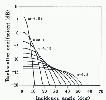
Fig. 10. Variations of the back-scatter coefficient as a function of incidence angle in the case of scattering by a large-scale roughness element. The curves are shown for various r.m.s. slopes of the roughness (m) from 0.05 to 0.5 (intervals of 0.05).
If a signal is observed at large incidence angles, it means that the surface roughness is small compared with the radar wavelength. The surface is then usually called a slightly rough surface of r.m.s. height σ1. It exists at least a correlation length l of the surface features smaller than the wavelength. This case corresponds to k1σ1 < 3. If some terms related to diffraction are neglected and incidence angles are larger than 25 °, the back-scatter coefficient is written (Reference FungFung, 1984)

p being the polarization (vertical or horizontal) and Rp the Fresnel coefficient. For horizontal polarization (Reference FungFung, 1984)

For vertical polarization (Reference FungFung, 1984)

W(2k1 sinθ) represents the roughness spectrum; that is, the Fourier transform of the surface height autocorrelation. If an exponential function is taken for the latter, this gives
The back-scatter coefficient is shown as a function ofθ for σ1 = 1 cm, ϵ = 1.8 and l varying from 1.2 to 4 cm (Fig. 11). Remember that the model is only valid at large incidence angles. The shape of the curve is essentially insensitive to l. The signal is more intense as the correlation length l decreases. Changing 鎵 within its range of values affects the intensity of the signal by only incidence to 3 dB at 60 ° incidence (Equation Equations (8) and Equation (9)). This is similar to the observations (Fig. 6). Note that Reference Swift, Hayes, Herd, Jones and DelnoreSwift and others (1985) argued that volume echo is dominant at large incidences because the micro-roughness creates polarization, which is not observed in airborne microwave measurements. However, the dielectric constant of the dry snow is such that the polarization effect is weak.

Fig. 11. Variations of the back-scatter coefficient with incidence angle in the case of back-scatter by a slightly rough surface. The model is only valid for θ larger than 25 °. The curves are shown for a given r.m.s. height of the roughness (σ = 1 cm) and for various length scales, I, from 1.2 to 4 cm (intervals of 0.2 cm).
Towards a Two-Scale Model for Surface-Echo Roughness
Variations of the back-scatter coefficient can be obtained for both small and large incidence angles. The large observed radar back-scatter intensity near the vertical is explained by a large-scale roughness model with a low surface slope r.m.s. (m of about 0.05 rad). On the other hand, in order to interpret the signal at large incidence angles, a small-scale roughness model is needed.
A two-scale roughness model is thus required, in which both micro-roughness and sastrugi would affect the radar echo. It is tempting to apply a two-scale roughness model, as for the ocean. We therefore use the theoretical model of Reference Chan and FungChan and Fung (1977), valid only for incidence angles greater than 30 ° and designed for the ocean case.
In this model, the back-scatter coefficient σpp due to small-scale roughness, described as a slightly rough surface, is averaged over the tilt θ′ created by the large-scale roughness.

where Zx
and Zy
arc the large-scale local surface slopes and ![]() is the large-scale slope distribution. The primes correspond to a reference system where the X′ axis
is the large-scale slope distribution. The primes correspond to a reference system where the X′ axis
In the case of Antarctica, the amplitude of the large-scale roughness would correspond to sastrugi. It is of the order of 10 cm to 1 m on distance scales of about 10 m. The corresponding slope would vary from 0 ° to 6 °. We will therefore neglect its effect, because it would correspond to a variation of the back-scatter coefficient of the order of only 1 dB. (This approximation should be verified using in-situ measurements of the slope statistics of the ice surface.) Then
and

The back-scatter coefficient is that of the small-scale surface-roughness model (Equation (7)) and

where Κ = 2k1 sin θ.
The spectrum for small-scale waves of the sea, the analogue of snow micro-roughness features, is known from observations and dynamical considerations. From this model spectrum, Reference Chan and FungChan and Fung (1977) derived the dependence of Wsea on azimuth as
where a is related to the ratio of the total slope variance across the wind direction to that up-wind.
Spectra for continental ice roughness are not available. However, as it is found experimentally that the back-scatter coefficient varies with azimuth as a bi-sinusoid (Fig. 8), the same functional dependence for Wice
(Equation (1)) is assumed. Note that, contrary to the ocean, where o is determined primarily by large-scale gravity waves, small-scale roughness may dominate the slope variances (in agreement with the previous simplifications for the calculation of ![]() .
.
The adjustments to the data were achieved as follows:
-
(i) The dependence on the azimuth was derived in each region from all data, including both polarizations and all incidence angles. This was done because the number of azimuth values is small for a given incidence angle and because no significant difference is found for region Β when the data set is split according to these parameters.
-
(ii) In the formula for the high incidence angle, small-scale roughness effect (Equation (7)), σl was fixed at 1.5 cm and l estimated by a least-squares fit to the observations. Only incidence angles larger than 25 ° were used (cells 1–12) and the calculations were done separately for each polarization. For θ > 25 °, a variation of l only changes the intensity of the back-scatter coefficient and not the shape of the curve (Fig. 13). As σl is a multiplicative constant, it would have the same effect. Thus, only the
 ratio can be estimated.
 -
(iii) Finally, using the large-scale roughness model (Equation (5)), the r.m.s. slope m was adjusted to the low incidence-angle data (cells 13–15). Of course, this is an approximation, because small-scale roughness also affects these values. However, the two effects are likely to be correlated. The results are summarized in Table 2.
Table 2. Roughness parameters as deduced by least-squares regression from the data, m is the r.m.s. surface slope, σ1 is the height r.m.s. for small-scale roughness and l the corresponding length scale. The regions have been ranked as in Table 1

The ![]() values for both polarizations are very consistent. They suggest that the typical scale height of roughness is twice as large for region Β than for the other regions (or alternatively that its length scale is less by half). The r.m.s. slope m varies accordingly. For a feature of 1 m scale height, its value implies a length scale of 6 m for region Β and of 12 m for regions A and D. This is consistent with typical scales for sastrugi. Note that aerial surveys of sastrugi typically report longer sastrugi than ground surveys, with length between 10 and 200 m (Reference Bromwich, Parish and ZormanBromwich and others, 1990).
values for both polarizations are very consistent. They suggest that the typical scale height of roughness is twice as large for region Β than for the other regions (or alternatively that its length scale is less by half). The r.m.s. slope m varies accordingly. For a feature of 1 m scale height, its value implies a length scale of 6 m for region Β and of 12 m for regions A and D. This is consistent with typical scales for sastrugi. Note that aerial surveys of sastrugi typically report longer sastrugi than ground surveys, with length between 10 and 200 m (Reference Bromwich, Parish and ZormanBromwich and others, 1990).
Discussion
Both surface-scattering at all incidence angles and volume-scattering at large incidence angles could explain the observations quantitatively. Note, however, that the surface and snow parameters should be correlated if both processes control the signal. It would be necessary for grain-size to be larger in areas of strong wind intensity to explain the larger signal in region Β at large incidence, and the correlation with emissivity at vertical polarization, by a volume-scattering effect. If this is the case, parameters for surface roughness and katabatic winds can be derived empirically using Equations Equation (5) and Equation (12). Note that “a” varies closely with the wind intensity (Table 1). The more intense is the wind, the more important the variations with the azimuth of observation relative to the wind direction. This leads us to argue that “a” is related to sastrugi, because these surface features increase in height with wind intensity (Reference Drewry, Mclntyre, Cooper and WoldenbergDrewry and others, 1985). On the other hand, m and σ2/l do not appear to be related to wind intensity alone (Table 2), except for region Β where the greater wind intensity will correspond to the higher values of these parameters. For the other cases, the value of m is not really distinct.
In any case, it would be necessary to study the statistics of the snow and its associated roughness parameters to develop more quantitative models of the scatterometer signal. Moreover, significant effects can be due to sub-surface layering, which may very well appear to simulate surface effects.
Conclusion
Above Antarctica, the back-scatter coefficient at 14.6 GHz, as measured by the Seasat scatterometer, varies in a way similar to that measured for the oceans. It decreases with incidence angle from 10 to −20 dB, and shows a signal of about +5 dB with the azimuth of observation relative to the wind direction (cf. Figs 2, 7 and 8). An important difference with the ocean case lies in the polarization of the signal, which is very small above ice (of the order ot 3 dB at most; Fig. 6), whereas it is larger than 10 dB above the ocean at high incidence angles (Fig. 2).
Simplified models of volume and surface back-scatter suggest that this signal could be explained by an effect of the latter. At low incidence angle, the signal depends mostly on the quadratic mean slope of the medium-scale surface features. Values of 0.08 to 0.16 are found, which can result from micro-roughness, sastrugi and snow dunes. The observed strong decrease of the signal with incidence angle completes the analysis of Reference Remy and MinsterRemy and Minster (1991), who used the altimeter measurements in the vertical. At high incidence angles (above 25 °), the signal would be dominated by micro-roughness. A characteristic parameter ![]() can be estimated, where σ1 is the r.m.s. height and l is the length scale of micro-roughness. It varies from 0.3 to 1 cm and increases with the intensity of katabatic winds.
can be estimated, where σ1 is the r.m.s. height and l is the length scale of micro-roughness. It varies from 0.3 to 1 cm and increases with the intensity of katabatic winds.
Unfortunately, the signal at high incidence angles could be explained as well by a volume back-scatter, provided the snow grain-size increases with surface-wind speed. In addition, this study cannot distinguish between pure surface effects and back-scatter from sub-surface layerings.
This preliminary study suggests that scatterometer observations above ice sheets provide an empirical mapping of roughness on various scales and may possibly lead to the identification of the surface-wind intensity and direction. This could be the first possible way to map the average surface winds in large, unmonitored areas of the continental ice sheets.
However, it also seems necessary to document the spectral characteristic of the surface roughness, as a function of wind speed and other parameters, in order to vinderstand this relationship. In addition to in-situ measurements, a more advanced model of the back-scatter is required. Such models now exist for the altimeter and for the scatterometer over land or vegetation. They should be easy to adapt to continental ice.
In any case, it would be interesting to obtain data for the back-scatter coefficient in various seasons and above all of the ice sheets. Thanks to sufficient power aboard the platform, the European Space Agency (ESA) recently decided to leave the ERS-1 scatterometer on over the whole Earth. This will provide dense, almost complete daily coverage of the Antarctic ice sheet with observations at many azimuth angles at each location. The instrument being in the C band rather than the KU band of the Seasat scatterometer, should diminish the volume effect by up to 15 dB. A number of our estimates will have to be re-evaluated, particularly with regard to the effects of micro-roughness. Very interesting results are to be expected from this data set.
Acknowledgements
We are grateful to Dr D. Bromwich for his many comments and suggestions in his review of this paper.
The accuracy of references in the text and in this list is the responsibility of the authors, to whom queries should be addressed.


