


1 Introduction
Since the works of Varley, Wheatstone and Siemens of around 1867, we know that electromagnetic dynamos can be self-excited, i.e. they work without permanent magnets to turn kinetic energy into electromagnetic energy. Unlike those technical dynamos with wires, homogeneous dynamos work in uniformly conducting media (Larmor Reference Larmor1919). They are prone to short-circuiting themselves, so for a long time it was unclear whether they could work at all. Indeed, it became clear that axisymmetric magnetic fields cannot be sustained by a dynamo (Cowling Reference Cowling1933). Axisymmetric flows, on the other hand, are capable of producing dynamos, but the resulting magnetic field is necessarily non-axisymmetric (Gailitis Reference Gailitis1970; Ponomarenko Reference Ponomarenko1973; Dudley & James Reference Dudley and James1989). Moss (Reference Moss1990) found that the critical magnetic Reynolds number, i.e. the ratio of inertial to resistive electromagnetic forces, is rather large for the dynamo of Gailitis (Reference Gailitis1970) to be excited. This means that the typical scale and velocity can be very large, so an experimental verification is difficult for that flow. For the Ponomarenko dynamo, by contrast, the critical magnetic Reynolds number is sufficiently low so that an experimental verification was successful (Gailitis et al. Reference Gailitis, Lielausis, Dementév, Platacis, Cifersons, Gerbeth, Gundrum, Stefani, Christen and Hänel2000).
Another self-excited dynamo arrangement that has been subjected to experimental verification is that of Herzenberg (Reference Herzenberg1958). The critical magnetic Reynolds number is again very large, but by using solid copper rotors that are in electric contact within a large copper block, it was possible to reach supercritical conditions (Lowes & Wilkinson Reference Lowes and Wilkinson1963, Reference Lowes and Wilkinson1968). Modelling the Herzenberg dynamo numerically has been possible by using relatively large rotors that are close together (Brandenburg, Moss & Soward Reference Brandenburg, Moss and Soward1998). From a numerical point of view, however, it is more advantageous to use periodic flow patterns. For example the Roberts flow I in a cubic domain has a critical magnetic Reynolds number of approximately 5 based on the root mean square (r.m.s.) velocity and the wavenumber of the flow. By comparison, the critical magnetic Reynolds number for the Arnold–Beltrami–Childress (ABC) flow (Galloway & Frisch Reference Galloway and Frisch1986) is approximately 15.
Indeed, certain periodic flows are better than others at producing dynamos. The optimal flow of ABC type, for example, was identified by Alexakis (Reference Alexakis2011). Other studies (Pringle & Kerswell Reference Pringle and Kerswell2010; Pringle, Willis & Kerswell Reference Pringle, Willis and Kerswell2012) on pipe flows led Willis (Reference Willis2012) to consider this as a variational problem. The optimal steady flow to excite a kinematic dynamo is found iteratively. Due to the arbitrarily low kinetic energy required to excite a dynamo (Proctor Reference Proctor2015), the magnetic Reynolds number should be based on the r.m.s. vorticity rather than the r.m.s. speed, which we refer to as  $R_{\unicode[STIX]{x1D714}}$ in this paper. A series of optimization studies followed. Chen, Herreman & Jackson (Reference Chen, Herreman and Jackson2015) considered physical boundary conditions, and Chen et al. (Reference Chen, Herreman, Li, Livermore, Luo and Jackson2018) applied the same method to a sphere. The optimal axisymmetric flow in a sphere has also been identified in the thesis of Chen (Reference Chen2018). All optimal flows have lowered the critical $R_{\unicode[STIX]{x1D714}}$ significantly.
It is often thought that some kind of swirl or helicity in the flow is important, but this is not generally true (Gilbert, Frisch & Pouquet Reference Gilbert, Frisch and Pouquet1988). Three of the four flows studied by Roberts (Reference Roberts1972) have no helicity and yet they can produce mean magnetic fields, as defined by planar averaging. In fact, different types of flow geometries can produce very different types of dynamos: small-scale dynamos, large-scale dynamos, those with an  $\unicode[STIX]{x1D6FC}$ effect and those without, etc. Non-helical isotropic turbulence only leads to small-scale dynamo action when the magnetic Reynolds number based on the r.m.s. speed exceeds a critical value that is between 40 and 200, depending on the magnetic Prandtl number – the ratio of kinematic viscosity to magnetic diffusivity (Iskakov et al. Reference Iskakov, Schekochihin, Cowley, McWilliams and Proctor2007; Brandenburg Reference Brandenburg2011). Those dynamos produce magnetic fields at scales as small as the resistive scale – the smallest scale where turbulent magnetic fields exist.
Some flows also act as large-scale dynamos, which produce magnetic fields that can be detected even after spatial averaging over certain directions. Such dynamos are also referred to as mean-field dynamos. Here we show that some of the optimal dynamos do indeed produce mean fields. We also examine the nature of such mean-field dynamo action.
2 Instructive examples of mean-field dynamos
A particularly famous example of a large-scale dynamo is the Roberts flow I, a flow with maximum kinetic helicity. The flow is of the form  $\boldsymbol{U}=k_{\text{f}}\unicode[STIX]{x1D713}\hat{\boldsymbol{z}}+\unicode[STIX]{x1D735}\times (\unicode[STIX]{x1D713}\hat{\boldsymbol{z}})$, where $\unicode[STIX]{x1D713}=\cos kx\cos ky$ is the stream function in Cartesian $(x,y,z)$ coordinates, $k$ is the wavenumber, and $k_{\text{f}}=\sqrt{2}k$ is the effective wavenumber (Roberts Reference Roberts1972). The critical magnetic Reynolds number, based on the r.m.s. velocity and the effective wavenumber $\sqrt{2}k$, is 3.9 for a domain of length $L=2\unicode[STIX]{x03C0}/k$ in the $z$ direction (Brandenburg & Subramanian Reference Brandenburg and Subramanian2005). Interestingly, a flow of the form $\boldsymbol{U}=k_{\text{f}}\unicode[STIX]{x1D713}\hat{\boldsymbol{z}}+\unicode[STIX]{x1D735}\times (\unicode[STIX]{x1D719}\hat{\boldsymbol{z}})$, where $\unicode[STIX]{x1D719}=\sin kx\sin ky$ is phase shifted in the $x$ and $y$ directions by $\unicode[STIX]{x03C0}/2$ relative to $\unicode[STIX]{x1D713}$ (Roberts flow II), has zero pointwise kinetic helicity. So, there is no swirl whatsoever, and yet, it produces not only a magnetic field, but one with non-vanishing $xy$ averages, although it requires $L\geqslant 2\unicode[STIX]{x03C0}/(0.64k)\approx 9.8/k$ (Rheinhardt et al. Reference Rheinhardt, Devlen, Rädler and Brandenburg2014).
In the following examples, we focus on dynamos that produce a non-vanishing mean field obtained by averaging over the  $xy$ plane of size $L^{2}$. This mean field is therefore defined as $\overline{\boldsymbol{B}}=\int \boldsymbol{B}\,\text{d}x\,\text{d}y/L^{2}$. In the case of Roberts flow I, the resulting mean field is of the form $\overline{\boldsymbol{B}}=B_{0}(t)(\sin (kz+\unicode[STIX]{x1D711}),\cos (kz+\unicode[STIX]{x1D711}),0)$, where $\unicode[STIX]{x1D711}$ is an arbitrary phase, $k$ is the wavenumber and $B_{0}(t)$ is a time-dependent amplitude. In the case of Roberts flow IV, the velocity has no net but still pointwise helicity. The mean magnetic field is time dependent and its $x$ and $y$ components evolve independently of each other, i.e.
 $$\begin{eqnarray}\overline{\boldsymbol{B}}(z,t)=(\overline{B}_{x},\overline{B}_{y},0)=(B_{0x}(t)\cos (k^{(x)}z+\unicode[STIX]{x1D711}_{x}),B_{0y}(t)\cos (k^{(y)}z+\unicode[STIX]{x1D711}_{y}),0),\end{eqnarray}$$
 where  $B_{0x}(t)$ and $B_{0y}(t)$ are time-dependent amplitudes, $\unicode[STIX]{x1D711}_{x}$ and $\unicode[STIX]{x1D711}_{y}$ are phases and $k^{(x)}$ and $k^{(y)}$ are wavenumbers for the $x$ and $y$ components, respectively. In principle, the values of $\overline{B}_{x}$ and $\overline{B}_{y}$ for a mean-field dynamo can be different from each other. For example, if $B_{0y}=0$, the magnetic field can just be $\overline{\boldsymbol{B}}=(B_{0x}\cos kz,0,0)$, i.e. with only one component. In fact, the Robert flows II–IV all produce dynamos where $\overline{B}_{x}$ and $\overline{B}_{y}$ evolve independently of each other, albeit at the same rate, i.e. $\text{d}\ln B_{0x}/\text{d}t=\text{d}\ln B_{0y}/\text{d}t$; see Devlen, Brandenburg & Mitra (Reference Devlen, Brandenburg and Mitra2013), Rheinhardt et al. (Reference Rheinhardt, Devlen, Rädler and Brandenburg2014). We are not aware of any earlier demonstration of a case where the growth rates of different components are not the same.
Solutions to large-scale or mean-field dynamos can be obtained if the mean electromotive force can be expressed in terms of the mean field. Here, the mean electromotive force is defined as  $\overline{\boldsymbol{{\mathcal{E}}}}=\overline{\boldsymbol{u}\times \boldsymbol{b}}$, where overbars denote $xy$ averaging and lowercase symbols denote fluctuations around the mean field, i.e. $\boldsymbol{u}=\boldsymbol{U}-\overline{\boldsymbol{U}}$ and $\boldsymbol{b}=\boldsymbol{B}-\overline{\boldsymbol{B}}$ are the fluctuating velocity and magnetic fields. The general relationship between $\overline{\boldsymbol{B}}$ and $\overline{\boldsymbol{{\mathcal{E}}}}$ is in terms of a convolution of the form
 $$\begin{eqnarray}\overline{\boldsymbol{{\mathcal{E}}}}=\iint K_{ij}(z-z^{\prime },t-t^{\prime })\,\overline{B}_{j}(z^{\prime },t^{\prime })\,\text{d}z^{\prime }\,\text{d}t^{\prime },\end{eqnarray}$$
 where  $K$ is an integral kernel. In the case of Roberts flow I, when the mean magnetic field is marginally excited, the kernel is approximately of the form
 $$\begin{eqnarray}K_{ij}(z,z^{\prime },t,t^{\prime })\approx \unicode[STIX]{x1D6FF}(z-z^{\prime })\unicode[STIX]{x1D6FF}(t-t^{\prime })(\unicode[STIX]{x1D6FC}\unicode[STIX]{x1D6FF}_{ij}-\unicode[STIX]{x1D702}_{\text{t}}\unicode[STIX]{x1D716}_{i3j}\unicode[STIX]{x2202}/\unicode[STIX]{x2202}z^{\prime }),\end{eqnarray}$$
 where  $\unicode[STIX]{x1D6FC}=(\unicode[STIX]{x1D702}+\unicode[STIX]{x1D702}_{\text{t}})k$ in the marginally excited case. In the case of Roberts flow II, the components of $K_{ij}$ cannot be described by an instantaneous relationship, but there is a turbulent pumping effect with a certain time delay (Rheinhardt et al. Reference Rheinhardt, Devlen, Rädler and Brandenburg2014). In this case, the $x$ and $y$ components evolve independently of each other. The dynamo for Roberts flow III is similar to that for Roberts flow II, except that the $x$ and $y$ components of the mean magnetic field experience pumping velocities that point in opposite directions.
Finally, Roberts flow IV is again given by an equation similar to (2.3), but with  $\unicode[STIX]{x1D6FC}=0$ and $\unicode[STIX]{x1D702}_{\text{t}}$ being negative on the length scales of interest. At smaller scales, however, $\unicode[STIX]{x1D702}_{\text{t}}$ is always positive, which is necessary so as to ensure stability at small length scales. This can be accounted for by adding a magnetic hyperdiffusivity, corresponding to an additional third-order spatial derivative term in (2.3). We return to this at the end of the paper. With these preparations in place, we are now in a position to characterize the dynamos driven by the aforementioned optimized flows.
In this study, we encounter examples of dynamos that share similarities with some of the cases discussed above. In particular, we find cases that do exhibit this type of unusual behaviour with two components evolving independently of each other. For example, the Willis dynamo is even more bizarre than that of Roberts flow IV, because the two horizontal components of  $\overline{\boldsymbol{B}}$ evolve differently, with growth rates that have even different signs. Robert flow I, by contrast, is maximally helical and leads to an $\unicode[STIX]{x1D6FC}$ effect that couples the two horizontal components of $\overline{\boldsymbol{B}}$. Those dynamos are called $\unicode[STIX]{x1D6FC}^{2}$ dynamos, because the $\unicode[STIX]{x1D6FC}$ effect is responsible for producing $\overline{B}_{x}$ from $\overline{B}_{y}$ and for producing $\overline{B}_{y}$ from $\overline{B}_{x}$. We talk about $\unicode[STIX]{x1D6FC}\unicode[STIX]{x1D6FA}$ dynamos when shear in (say) the $y$ direction ( $\unicode[STIX]{x1D6FA}$ effect) is responsible for producing $\overline{B}_{y}$ from $\overline{B}_{x}$. The flows of Willis (Reference Willis2012) and Chen et al. (Reference Chen, Herreman and Jackson2015) turn out not to be of that type. Below, we present a more detailed analysis of these optimal dynamos.
3 Essentials of dynamos driven by optimized flow
The goal of this study is to determine the nature of dynamo action driven by the flows of Willis (Reference Willis2012) and Chen et al. (Reference Chen, Herreman and Jackson2015). We discuss three types of optimal flows with distinct boundary conditions for their excited magnetic eigenmodes, referred to as Willis, NNT and TTT cases. In Chen et al. (Reference Chen, Herreman and Jackson2015), the magnetic boundary conditions can be either superconducting or pseudo-vacuum in each direction. In terms of spectral representations, this means either using sine functions (T for tangential) or cosine functions (N for normal) in the direction perpendicular to the boundary. The corresponding magnetic eigenmodes then have four possible combinations: NNT, NTT, NNN, and TTT in  $x,y,z$ respectively. The NNT/NTT and NNN/TTT pairs give the same dynamo up to a symmetry transformation (Favier & Proctor Reference Favier and Proctor2013). Thus, only one solution from each pair is chosen for this study. We begin by briefly explaining the essential technique to obtaining these optimal flows, and then describe the dominant Fourier modes of the dynamo solution, if there is any.
Basically, the optimization method belongs to the family of constrained optimizations. Given a Lagrangian as follows,
 $$\begin{eqnarray}\displaystyle {\mathcal{L}} & = & \displaystyle \ln \langle \boldsymbol{B}_{T}^{2}\rangle -\unicode[STIX]{x1D706}_{1}(\langle \unicode[STIX]{x1D74E}^{2}\rangle -1)-\unicode[STIX]{x1D706}_{2}(\langle \boldsymbol{B}_{0}^{2}\rangle -1)-\langle \unicode[STIX]{x1D6F1}_{1}\,\unicode[STIX]{x1D735}\boldsymbol{\cdot }\boldsymbol{U}\rangle -\langle \unicode[STIX]{x1D6F1}_{2}\unicode[STIX]{x1D735}\boldsymbol{\cdot }\boldsymbol{B}_{0}\rangle \nonumber\\ \displaystyle & & \displaystyle -\,\int _{0}^{\text{T}}\langle \boldsymbol{B}^{\dagger }\boldsymbol{\cdot }[\unicode[STIX]{x2202}_{t}\boldsymbol{B}-\unicode[STIX]{x1D735}\times (\boldsymbol{U}\times \boldsymbol{B})-R_{\unicode[STIX]{x1D714}}^{-1}\unicode[STIX]{x1D6FB}^{2}\boldsymbol{B}]\rangle \,\text{d}t,\end{eqnarray}$$
 where  $\unicode[STIX]{x1D74E}=\unicode[STIX]{x1D735}\times \boldsymbol{U}(\boldsymbol{x})$, $\boldsymbol{B}_{T}=\boldsymbol{B}(\boldsymbol{x},T)$, $\langle \cdots \rangle =V^{-1}\int \cdots \text{d}V$ denotes the volume average and $T$ is a fixed time that is long enough to filter out a transient growth. The first term in (3.1) is a proxy of the growth rate that we want to maximize, whilst the other terms are constraints from a kinematic dynamo model (the backreaction from the magnetic field on the flow is not considered). We search for the optimal flow $\boldsymbol{U}$ and the initial field $\boldsymbol{B}_{0}$ such that all variations vanish
 $$\begin{eqnarray}\unicode[STIX]{x1D6FF}{\mathcal{L}}(\boldsymbol{U},\boldsymbol{B},\boldsymbol{B}^{\dagger },\boldsymbol{B}_{0},\boldsymbol{B}_{T},\unicode[STIX]{x1D706}_{1},\unicode[STIX]{x1D706}_{2},\unicode[STIX]{x1D6F1}_{1},\unicode[STIX]{x1D6F1}_{2})=0.\end{eqnarray}$$
 Setting  $\unicode[STIX]{x1D6FF}{\mathcal{L}}/\unicode[STIX]{x1D6FF}\boldsymbol{B}^{\dagger }=0$ gives the induction equation
 $$\begin{eqnarray}\unicode[STIX]{x2202}_{t}\boldsymbol{B}=\unicode[STIX]{x1D735}\times (\boldsymbol{U}\times \boldsymbol{B})+R_{\unicode[STIX]{x1D714}}^{-1}\unicode[STIX]{x1D6FB}^{2}\boldsymbol{B},\end{eqnarray}$$
 and setting  $\unicode[STIX]{x1D6FF}{\mathcal{L}}/\unicode[STIX]{x1D6FF}\boldsymbol{B}=0$ gives the adjoint induction equation,
 $$\begin{eqnarray}\unicode[STIX]{x2202}_{t}\boldsymbol{B}^{\dagger }=\boldsymbol{U}\times (\unicode[STIX]{x1D735}\times \boldsymbol{B}^{\dagger })-R_{\unicode[STIX]{x1D714}}^{-1}\unicode[STIX]{x1D6FB}^{2}\boldsymbol{B}^{\dagger }.\end{eqnarray}$$
 The optimization procedure is based on the two equations above. Starting from some fields  $\boldsymbol{U}$ and $\boldsymbol{B}_{0}$, we first evolve the system forward in time using (3.3) until time $T$, then backward in time using (3.4) and finally we use $\unicode[STIX]{x1D6FF}{\mathcal{L}}/\unicode[STIX]{x1D6FF}\boldsymbol{U}$ and $\unicode[STIX]{x1D6FF}{\mathcal{L}}/\unicode[STIX]{x1D6FF}\boldsymbol{B}_{0}$ as gradients to update $\boldsymbol{U}$ and $\boldsymbol{B}_{0}$. A detailed optimization algorithm is described in Chen et al. (Reference Chen, Herreman and Jackson2015).
The resulting optimal flow  $\boldsymbol{U}$ and the corresponding least decaying magnetic eigenmode show drastically different features for the three cases we are interested in. The Willis case represents the most efficient solution (has lowest critical $R_{\unicode[STIX]{x1D714}}$) with periodic boundary conditions for the flow and the magnetic eigenmode. Since the optimization algorithm does not fix the orientation of fields, any transformation such as shift ( $T_{\unicode[STIX]{x1D6FF}}$), rotation, or reflection ( ${\mathcal{R}}$) gives the same equivalent optimal flows,
 $$\begin{eqnarray}\boldsymbol{U}(\boldsymbol{x})={\mathcal{R}}^{-1}\widetilde{\boldsymbol{U}}(\tilde{\boldsymbol{x}}(\boldsymbol{x})),\end{eqnarray}$$
 where  $\tilde{\boldsymbol{x}}(\boldsymbol{x})={\mathcal{R}}\boldsymbol{x}+T_{\unicode[STIX]{x1D6FF}}$ gives the relation of two coordinates. Here, tildes denote quantities in the original coordinate. The Willis flow can be approximately described by a large-scale dominant flow (up to 1 % difference in the vorticity norm $\Vert \unicode[STIX]{x1D714}\Vert _{2}$) in the original coordinate as
 $$\begin{eqnarray}\frac{\widetilde{\boldsymbol{U}}}{\tilde{U} _{\text{rms}}}\approx \frac{2}{\sqrt{3}}(\sin {\tilde{y}}\cos \tilde{z},\sin \tilde{z}\cos \tilde{x},\sin \tilde{x}\cos {\tilde{y}}).\end{eqnarray}$$
For the flow we use, the actual form in the transformed coordinate is
 $$\begin{eqnarray}\frac{\boldsymbol{U}}{U_{\text{rms}}}\approx \frac{2}{\sqrt{3}}(\sin (z+\unicode[STIX]{x03C0}/2)\cos (y-\unicode[STIX]{x03C0}/4),\sin x\cos (z+\unicode[STIX]{x03C0}/2),\sin (y-\unicode[STIX]{x03C0}/4)\cos x).\end{eqnarray}$$
 The two sets of coordinates are related by  $(\tilde{x},{\tilde{y}},\tilde{z})=(x,z+\unicode[STIX]{x03C0}/2,y-\unicode[STIX]{x03C0}/4)$. The magnetic eigenmode of this dynamo can also be approximated by a simple field (up to 2 % difference in energy) as
 $$\begin{eqnarray}\boldsymbol{B}_{T}\approx \left[\begin{array}{@{}c@{}}0.138\cos z+0.810\sin z\\ -0.802\cos x+0.179\sin x\\ -0.538\cos y-0.622\sin y\end{array}\right],\end{eqnarray}$$
 in the transformed coordinate. The  $x,y,z$ components of (3.8) each vary only in one direction. If small fluctuations are added to this eigenmode, we would expect to find a non-zero mean field when taking any of the planar averages.
In Chen et al. (Reference Chen, Herreman and Jackson2015), a combination of sine and cosine functions is used to mimic physical boundary conditions in a domain of size 1. The flow satisfies non-penetrating boundary conditions and therefore only sine functions are allowed in the direction perpendicular to the boundary. In this study, we rescale the flows of Chen et al. (Reference Chen, Herreman and Jackson2015) such that they become periodic in a  $(2\unicode[STIX]{x03C0})^{3}$ domain while retaining the boundary conditions in a $\unicode[STIX]{x03C0}^{3}$ domain. In the extended $(2\unicode[STIX]{x03C0})^{3}$ domain, the general form is given by
 $$\begin{eqnarray}\boldsymbol{U}=\mathop{\sum }_{m_{x},m_{y},m_{z}\in \mathbb{N}}\left[\begin{array}{@{}c@{}}a_{x}(m_{x},m_{y},m_{z})\sin (m_{x}x)\cos (m_{y}y)\cos (m_{z}z)\\ a_{y}(m_{x},m_{y},m_{z})\cos (m_{x}x)\sin (m_{y}y)\cos (m_{z}z)\\ a_{z}(m_{x},m_{y},m_{z})\cos (m_{x}x)\cos (m_{y}y)\sin (m_{z}z)\end{array}\right],\end{eqnarray}$$
 and  $a_{i}(m_{x},m_{y},m_{z})$ with $i=x,y,z$ being the spectral coefficients. This is similar to the Taylor–Green flow but with the sine and cosine functions swapped. The NNT magnetic field has the general form
 $$\begin{eqnarray}\boldsymbol{B}_{\text{NNT}}^{\prime }=\mathop{\sum }_{m_{x},m_{y},m_{z}\in \mathbb{N}}\left[\begin{array}{@{}c@{}}a_{x}(m_{x},m_{y},m_{z})\cos (m_{x}x)\sin (m_{y}y)\cos (m_{z}z)\\ a_{y}(m_{x},m_{y},m_{z})\sin (m_{x}x)\cos (m_{y}y)\cos (m_{z}z)\\ a_{z}(m_{x},m_{y},m_{z})\sin (m_{x}x)\sin (m_{y}y)\sin (m_{z}z)\end{array}\right],\end{eqnarray}$$
 which corresponds to normal field boundary conditions in the  $x$ and $y$ directions, and perfectly conducting boundaries in the $z$ direction; $\boldsymbol{B}_{\text{TTT}}^{\prime }$ has the same general representation as (3.9). This is because the boundary conditions for both fields forbid normal components across the boundary, but allow tangential components.
To distinguish the two cases, the optimal flows are named after the boundary conditions of their corresponding magnetic eigenmodes. For up to 83 % of the total enstrophy,  $\langle \unicode[STIX]{x1D74E}^{2}\rangle$, the optimal NNT flow can be approximated by the velocity $\boldsymbol{U}\approx \unicode[STIX]{x1D735}\times \unicode[STIX]{x1D74D}$ with
 $$\begin{eqnarray}\left[\begin{array}{@{}c@{}}\unicode[STIX]{x1D713}_{x}(x,y,z)\\ \unicode[STIX]{x1D713}_{y}(x,y,z)\\ \unicode[STIX]{x1D713}_{z}(x,y,z)\end{array}\right]=\left[\begin{array}{@{}cc@{}}0.16 & \sin 2y\sin 2z\\ 0.77 & \sin x\sin z\\ -0.18 & \sin 2x\sin 2y\end{array}\right].\end{eqnarray}$$
The leading components of the magnetic eigenmode are given in Chen et al. (Reference Chen, Herreman and Jackson2015). In particular, the most energetic Fourier mode takes 39 % of the total energy, and varies only in one direction
 $$\begin{eqnarray}{B_{x}^{\prime }}_{\text{NNT}}(0,1,0)=0.883\sin y,\end{eqnarray}$$
 where  $(0,1,0)$ are the wavenumbers in $x,y,z$ respectively. We expect to see some contribution from $B_{x}^{\prime }$ for the $xz$ averages taken in the $(2\unicode[STIX]{x03C0})^{3}$ domain. The other dominant Fourier components depend on at least two directions, hence have zero planar averages.
The TTT case has neither a dominant flow nor a dominant magnetic field that varies only in one direction. The optimal TTT flow is highly localized, but has approximately equal enstrophy per direction ( $\langle \unicode[STIX]{x1D714}_{i}^{2}\rangle ,i=x,y,z$); see also Chen et al. (Reference Chen, Herreman and Jackson2015) for the streamline plot. We do not expect to find a planar mean field near onset for this type of dynamo.
With three types of boundary conditions, we get three optimal solutions: the Willis and NNT dynamos both have simple large-scale flows, except the NNT dynamo breaks the symmetry in one direction, and the TTT dynamo has a complex localized flow. These three dynamo solutions were computed without imposing specific physical properties of the flow a priori. While this approach allows us to remove bias and explore the full parameter space of solutions, it leaves the question of how to interpret the dynamo action. In the next section, we discuss how to extend the analysis of dynamos using mean-field theories.
4 Mean-field approaches to analysing the dynamos
To characterize the nature of dynamo action for the three optimized flow problems, we use both direct numerical simulations (DNS) and the test-field method (TFM). The DNS refer to the numerical solution of (3.3), whereas the TFM refers to solutions of the evolution equations for the fluctuations around a given planar averaged mean field, which is one of four test fields,  $\overline{\boldsymbol{B}}^{\text{T}}$. The TFM allows us to extract turbulent transport coefficients from the underlying flow fields (Schrinner et al. Reference Schrinner, Rädler, Schmitt, Rheinhardt and Christensen2005, Reference Schrinner, Rädler, Schmitt, Rheinhardt and Christensen2007); see also Brandenburg et al. (Reference Brandenburg, Chatterjee, Del Sordo, Hubbard, Käpylä and Rheinhardt2010) for a review. We use numerical representations of the flows of Chen et al. (Reference Chen, Herreman and Jackson2015) for NNT and TTT dynamos in their original form, i.e. the r.m.s. of velocity is unnormalized, but we extend the domain to $(2\unicode[STIX]{x03C0})^{2}$ to match the periodic boundaries and also to reproduce Willis dynamo using a similar algorithm. The corresponding data files for these three flow fields can be found in the online material (Brandenburg & Chen Reference Brandenburg and Chen2019) for the published data sets used to compute each of the figures of the present paper. For comparison, we also use the original formulation of Willis (Reference Willis2012), denoted by Willis* (with an asterisk), which is written as $\boldsymbol{U}=(2/\sqrt{3})(\sin y\cos z,\sin z\cos x,\sin x\cos y)$ in the same coordinate as other flows, as opposed to the transformed form in (3.7). All these flows and the resulting magnetic fields are periodic in the $(2\unicode[STIX]{x03C0})^{3}$ volume, but for the NNT and TTT cases, we also select a $\unicode[STIX]{x03C0}^{3}$ subvolume with the appropriate boundary conditions. The flows are represented on a $32^{3}$ mesh, except for the TTT case, which is represented on a $48^{3}$ mesh. For the NNT and TTT cases in $\unicode[STIX]{x03C0}^{3}$ subvolumes, we select the first $17^{3}$ and $25^{3}$ mesh points, respectively, which include the points on the boundaries.
4.1 Characterizing the growth of the mean field
The growth of the mean field can be characterized through averaging. From the kinematic model, we know the spatial distribution of the magnetic eigenmode. The choice of averaging is then determined by the dominant magnetic field components. We take  $xy$ averages for the Willis and TTT cases, and $xz$ averages for the NNT case, and denote those by an overbar. To compute r.m.s. values, we employ volume averages, denoted by angle brackets. The r.m.s. values of the velocity, $U_{\text{rms}}\equiv \langle \boldsymbol{U}^{2}\rangle ^{1/2}$, are listed in table 1. The kinetic helicity integrated over the full domain is zero, but its local value at arbitrary points in the domain is finite. For the NNT flow, the kinetic helicity integrated over the $\unicode[STIX]{x03C0}^{3}$ domain is also zero. By contrast, the TTT flow lacks the symmetry to have a net zero helicity in the $\unicode[STIX]{x03C0}^{3}$ domain.
To obtain  $\boldsymbol{B}=\unicode[STIX]{x1D735}\times \boldsymbol{A}$, we solve for the magnetic vector potential $\boldsymbol{A}$. Its evolution is governed by the uncurled induction equation,
 $$\begin{eqnarray}\frac{\unicode[STIX]{x2202}\boldsymbol{A}}{\unicode[STIX]{x2202}t}=\boldsymbol{U}\times \boldsymbol{B}+\unicode[STIX]{x1D702}\unicode[STIX]{x1D6FB}^{2}\boldsymbol{A}.\end{eqnarray}$$
We solve this equation using the Pencil CodeFootnote 1, which is a high-order public domain code for solving partial differential equations, including the induction equation that is of interest here, as well as the test-field equations that are discussed in the next section. The code uses sixth order finite differences in space and the third-order low storage Runge–Kutta time stepping scheme of Williamson (Reference Williamson1980).
Table 1. Summary of parameters for various flows. For the 15 % supercritical cases, the values of  $q\equiv \overline{B}_{\text{rms}}/B_{\text{rms}}$ are given along with the corresponding values of $\unicode[STIX]{x1D702}$ (sixth column), the growth rate $\unicode[STIX]{x1D706}$ of the r.m.s. magnetic field and those of the mean-field components $\overline{B}_{x}$ and $\overline{B}_{y}$ (or $\overline{B}_{z}$ for the $xz$ averaged NNT flow), denoted by $\unicode[STIX]{x1D706}_{\text{mean}}^{(x)}$ and $\unicode[STIX]{x1D706}_{\text{mean}}^{(y,z)}$, respectively. Their imaginary parts give the frequency of oscillatory field components. The asterisk on the value 0.45 for $q$ denotes that a columnar $z$ average has been used in this case (see text).

When  $\unicode[STIX]{x1D702}$ is below a certain critical value, $\unicode[STIX]{x1D702}_{\text{crit}}$, the value of the r.m.s. magnetic field, $B_{\text{rms}}$, grows exponentially proportional to $e^{\unicode[STIX]{x1D706}t}$ where $\unicode[STIX]{x1D706}$ is a constant. For oscillatory fields, $\unicode[STIX]{x1D706}$ can be complex such that $2\unicode[STIX]{x03C0}/\text{Im}\,\unicode[STIX]{x1D706}$ is the period of the oscillation, and $\text{Re}\,\unicode[STIX]{x1D706}$ is the growth rate, which can be estimated from the logarithmic derivative of $B_{\text{rms}}$ or its envelope for oscillatory fields. By experimenting with different values of $\unicode[STIX]{x1D702}$, and by interpolation, we find the critical value $\unicode[STIX]{x1D702}_{\text{crit}}$ below which the dynamo is excited.
4.2 Quantitative analysis using the TFM
The averaged evolution or mean-field equation reads
 $$\begin{eqnarray}\frac{\unicode[STIX]{x2202}\overline{\boldsymbol{A}}}{\unicode[STIX]{x2202}t}=\overline{\boldsymbol{U}}\times \overline{\boldsymbol{B}}+\overline{\boldsymbol{{\mathcal{E}}}}+\unicode[STIX]{x1D702}\unicode[STIX]{x1D6FB}^{2}\overline{\boldsymbol{A}},\end{eqnarray}$$
 where  $\overline{\boldsymbol{{\mathcal{E}}}}=\overline{\boldsymbol{u}\times \boldsymbol{b}}$ is the electromotive force from the fluctuating velocity and magnetic fields, $\boldsymbol{b}=\unicode[STIX]{x1D735}\times \boldsymbol{a}$ is the small-scale magnetic field and $\boldsymbol{a}$ is a solution to the equation that results by subtracting (4.2) from (4.1), which yields
 $$\begin{eqnarray}\frac{\unicode[STIX]{x2202}\boldsymbol{a}}{\unicode[STIX]{x2202}t}=\overline{\boldsymbol{U}}\times \boldsymbol{b}+\boldsymbol{u}\times \overline{\boldsymbol{B}}+\boldsymbol{{\mathcal{E}}}^{\prime }+\unicode[STIX]{x1D702}\unicode[STIX]{x1D6FB}^{2}\boldsymbol{a},\end{eqnarray}$$
 where  $\boldsymbol{{\mathcal{E}}}^{\prime }=\boldsymbol{{\mathcal{E}}}-\overline{\boldsymbol{{\mathcal{E}}}}$ is the fluctuation of the electromotive force. This equation contains $\overline{\boldsymbol{B}}$, but it can also be formulated for arbitrary mean fields, which we then call test fields, $\overline{\boldsymbol{B}}^{\text{T}}$. The goal is to determine solutions to this equation for sufficiently many independent test fields so that we can assemble all eight unknowns, $\tilde{\unicode[STIX]{x1D6FC}}_{ij}$ and $\tilde{\unicode[STIX]{x1D702}}_{ij}$, for $i,j=1,2$ to the equation
 $$\begin{eqnarray}\tilde{{\mathcal{E}}}_{i}^{\text{T}}=\tilde{\unicode[STIX]{x1D6FC}}_{ij}\overline{B}_{j}^{\text{T}}-\tilde{\unicode[STIX]{x1D702}}_{ij}\overline{J}_{j}^{\text{T}},\end{eqnarray}$$
 where  $\overline{\boldsymbol{J}}^{\text{T}}=\unicode[STIX]{x1D735}\times \overline{\boldsymbol{B}}^{\text{T}}$. In general, the actual mean fields are neither constant in space nor in time, so we need to sample all Fourier modes in $z$ and $t$ to capture the full dependence. (Here, and in the following, we mean $y$ instead of $z$ when dealing with the NNT flow.) Fourier-transformed variables are denoted by tildes. The electromotive force is then written in the form (Brandenburg, Rädler & Schrinner Reference Brandenburg, Rädler and Schrinner2008)
 $$\begin{eqnarray}\tilde{{\mathcal{E}}}_{i}(z,t)=\int [\tilde{\unicode[STIX]{x1D6FC}}_{ij}(z,t,k,\unicode[STIX]{x1D714})\tilde{B}_{j}(k,\unicode[STIX]{x1D714})-\tilde{\unicode[STIX]{x1D702}}_{ij}(z,t,k,\unicode[STIX]{x1D714})\tilde{J}_{j}(k,\unicode[STIX]{x1D714})]\,\text{d}k\,\text{d}\unicode[STIX]{x1D714}.\end{eqnarray}$$
 The  $z$ profiles of all components of $\tilde{\unicode[STIX]{x1D6FC}}_{ij}(z,t,k,\unicode[STIX]{x1D714})$ and $\tilde{\unicode[STIX]{x1D702}}_{ij}(z,t,k,\unicode[STIX]{x1D714})$ are obtained by solving the test-field equations for different values of $k$ and $\unicode[STIX]{x1D714}$, where $k$ is the wavenumber and $\unicode[STIX]{x1D714}$ is the frequency in Fourier space.
Here,  $\tilde{\boldsymbol{B}}=\int \text{e}^{-\text{i}(kz-\unicode[STIX]{x1D714}t)}\overline{\boldsymbol{B}}\,\text{d}z\,\text{d}t$ is the Fourier-transformed mean field, and likewise for $\tilde{\boldsymbol{J}}$. For determining $\tilde{\unicode[STIX]{x1D6FC}}_{ij}$ and $\tilde{\unicode[STIX]{x1D702}}_{ij}$, we solve four copies of (4.3), each with one of four different test fields; $\overline{\boldsymbol{B}}^{\text{T}}=(\sin kz,0,0)$, $(\cos kz,0,0)$, $(0,\sin kz,0)$ and $(0,\cos kz,0)$. We then solve the test-field equation forward in time. Given that $\boldsymbol{U}$ is constant in time, we can use a relaxation method (see Rheinhardt et al. Reference Rheinhardt, Devlen, Rädler and Brandenburg2014, for details) and rewrite the test field as $\overline{\boldsymbol{B}}^{\text{T}}\rightarrow \text{e}^{-\text{i}\unicode[STIX]{x1D714}t}\hat{\boldsymbol{B}}^{\text{T}}(z;\unicode[STIX]{x1D714})$. This notation is not to be confused with the solutions to the adjoint problem, $\boldsymbol{B}^{\dagger }$, discussed in § 3.
We solve the Fourier-transformed complex equations for the response to each of the test fields. Those equations are given by (Rheinhardt et al. Reference Rheinhardt, Devlen, Rädler and Brandenburg2014)
 $$\begin{eqnarray}\text{i}\unicode[STIX]{x1D714}\tilde{\boldsymbol{a}}^{\text{T}}+\boldsymbol{u}\times \hat{\boldsymbol{B}}^{\text{T}}+(\boldsymbol{u}\times \tilde{\boldsymbol{b}}^{\text{T}})^{\prime }+\unicode[STIX]{x1D702}\unicode[STIX]{x1D6FB}^{2}\tilde{\boldsymbol{a}}^{\text{T}}=0,\end{eqnarray}$$
 where  $\tilde{\boldsymbol{b}}^{\text{T}}=\unicode[STIX]{x1D735}\times \tilde{\boldsymbol{a}}^{\text{T}}$ are the solutions, tildes denote Fourier transform in time, $\tilde{\boldsymbol{a}}^{\text{T}}(\boldsymbol{x},\unicode[STIX]{x1D714})=\int \boldsymbol{a}^{\text{T}}(\boldsymbol{x},t)\text{e}^{-\text{i}\unicode[STIX]{x1D714}t}\,\text{d}t$ and lowercase letters and primes denote fluctuations about the planar average. We then compute the desired transport coefficients in Fourier space, $\tilde{\unicode[STIX]{x1D6FC}}_{ij}$ and $\tilde{\unicode[STIX]{x1D702}}_{ij}$ by measuring $\tilde{\boldsymbol{{\mathcal{E}}}}^{\text{T}}=\overline{\boldsymbol{u}\times \tilde{\boldsymbol{b}}^{\text{T}}}$ and then solving (4.4). The diagonal components of the sum $\unicode[STIX]{x1D702}+\tilde{\unicode[STIX]{x1D702}}_{ij}$ act as an effective magnetic diffusivity, which has to be overcome by the other inductive effects in order for mean-field dynamo action to occur. We apply the complex TFM to the three optimal flows discussed earlier.
5 DNS results and spatial averages for the different dynamos
The critical magnetic diffusivity,  $\unicode[STIX]{x1D702}_{\text{crit}}$, along with the r.m.s. velocities and other relevant parameters such as the critical magnetic Reynolds numbers,
 $$\begin{eqnarray}R_{\text{m}}^{\text{crit}}=u_{\text{rms}}/\unicode[STIX]{x1D702}_{\text{crit}}k_{1},\end{eqnarray}$$
 are listed in table 1. Here  $k_{1}$ is an estimate of the relevant wavenumber of the magnetic field – usually the lowest in the domain. We use $k_{1}=1$ in all cases, and fluctuations are periodic. We also list the ratio $q\equiv \overline{B}_{\text{rms}}/B_{\text{rms}}$ of the r.m.s. values of the mean field, $\overline{B}_{\text{rms}}$, to that of the full field, $B_{\text{rms}}$, for cases that are approximately 15 % supercritical. The Karlsruhe and Riga dynamo experiments were only approximately 10 % supercritical, as measured by the magnetic Reynolds number based on the characteristic flow speed (Gailitis et al. Reference Gailitis, Lielausis, Platacis, Gerbeth and Stefani2003; Dormy & Soward Reference Dormy and Soward2007). Testing the near-critical response of the mean field is, therefore, a useful way of characterizing a weakly supercritical dynamo. In table 1, we also list the growth rates $\unicode[STIX]{x1D706}$ of the actual field $|\boldsymbol{B}|$ and $\unicode[STIX]{x1D706}_{\text{mean}}^{(i)}$ of the $i$th component of the mean field $\overline{B}_{i}$. Negative values indicate decay and an imaginary part denotes the frequency for oscillatory behaviour.
For comparison, we have included in table 1 the results for the more familiar ABC and Roberts flows. The ABC flow (Childress Reference Childress1970) is given by  $\boldsymbol{U}=(\sin z+\cos y,\sin x+\cos z,\sin y+\cos x)$. The equation for the ABC flow is similar to that for the Willis flow, except that the multiplications in the latter are replaced by plus signs in the ABC flow.
5.1 Dynamo action in the Willis dynamo
For the analytically given flow Willis*, which has a r.m.s. velocity of unity, we find mean-field dynamo action for  $\unicode[STIX]{x1D702}<\unicode[STIX]{x1D702}_{\text{crit}}=0.568$. This corresponds to $R_{\text{m}}^{\text{crit}}=1.76$. For the numerically optimized flow ‘Willis’ (without asterisk), which we focus on in the rest of this paper, the r.m.s. velocity is smaller and $\unicode[STIX]{x1D702}_{\text{crit}}=0.403$. This corresponds to $R_{\text{m}}^{\text{crit}}=1.75$, so it is only slightly easier to excite than Willis*. The following considerations apply all to the latter, numerically optimized flow. In the supercritical case, here using $\unicode[STIX]{x1D702}=0.35$, all three components of $\boldsymbol{B}$ are seen to grow exponentially in time at the rate $\unicode[STIX]{x1D706}\approx 0.052$; see figure 1.
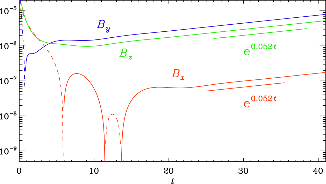
Figure 1. The three components of the magnetic field,  $B_{x}$ (red), $B_{y}$ (blue) and $B_{z}$ (green), at an arbitrarily selected point $\boldsymbol{x}_{\ast }$ within the domain for the Willis flow with $\unicode[STIX]{x1D702}=0.35$, which is supercritical. All three components begin to grow exponentially at the same rate. Solid (dashed) lines denote positive (negative) values.
For the Willis flow, as we will see below, equation (4.1) possesses solutions with non-vanishing planar or  $xy$ averages. It turns out that there is a finite mean field, $\overline{\boldsymbol{B}}(z_{\ast },t)$, where $z_{\ast }$ is a fixed position. In figure 2, we show its $x$ and $y$ components. Note that $\overline{B}_{z}=0$ at all times owing to the fact that $\unicode[STIX]{x1D735}\boldsymbol{\cdot }\overline{\boldsymbol{B}}=\unicode[STIX]{x2202}\overline{B}_{z}/\unicode[STIX]{x2202}z=0$ and that the mean field was vanishing initially. We see that $\overline{B}_{x}(z_{\ast },t)$ grows with the same growth rate as the actual magnetic field at any arbitrarily selected point (see figure 1), but $\overline{B}_{y}(z_{\ast },t)$ is seen to decay in an oscillatory fashion with frequency $\text{Im}\,\unicode[STIX]{x1D706}\approx 0.58$ at a rate $\text{Re}\,\unicode[STIX]{x1D706}_{\text{mean}}^{(y)}\approx -0.26$. The occurrence of different growth rates for different components is unusual and very different from the more familiar $\unicode[STIX]{x1D6FC}^{2}$ and $\unicode[STIX]{x1D6FC}\unicode[STIX]{x1D6FA}$ dynamos (Krause & Rädler Reference Krause and Rädler1980), where two components (poloidal and toroidal fields) always evolve in tandem. For example, the previously mentioned Roberts flow I is of $\unicode[STIX]{x1D6FC}^{2}$ type, but the dynamos from flows II and III work with time delay, and flow IV generates a negative diffusivity dynamo. The different behaviours between standard $\unicode[STIX]{x1D6FC}^{2}$ and $\unicode[STIX]{x1D6FC}\unicode[STIX]{x1D6FA}$ dynamos on the one hand and negative turbulent diffusivity and time delay dynamos on the other hand is illustrated in figure 3.

Figure 2. Evolution of  $\overline{B}_{x}(z_{\ast },t)$ (red) and $\overline{B}_{y}(z_{\ast },t)$ (blue) for the Willis flow at a fixed position $z_{\ast }$. Note that $\overline{B}_{y}$ decays in an oscillatory fashion with the frequency $\text{Im}\,\unicode[STIX]{x1D706}=0.58$. Again, solid (dashed) lines denote positive (negative) values.

Figure 3. Sketch illustrating the mutual feedbacks between  $\overline{B}_{x}$ and $\overline{B}_{y}$ in $\unicode[STIX]{x1D6FC}^{2}$ or $\unicode[STIX]{x1D6FC}\unicode[STIX]{x1D6FA}$ dynamos (a), and the independent evolution of the two components in negative turbulent diffusivity and time delay dynamos (b). For negative turbulent diffusivity dynamos, the growth rate of $\overline{B}_{x}$ is $-(\unicode[STIX]{x1D702}+\tilde{\unicode[STIX]{x1D702}}_{yy})k^{2}$ and that of $\overline{B}_{y}$ is $-(\unicode[STIX]{x1D702}+\tilde{\unicode[STIX]{x1D702}}_{xx})k^{2}$, and they can be different from each other.
To understand the negative turbulent diffusivity dynamos, we emphasize that, in view of (4.2) and (4.5),  $\tilde{\unicode[STIX]{x1D702}}_{xx}$ affects the evolution of $\overline{A}_{x}$ and thus $\overline{B}_{y}=\unicode[STIX]{x2202}\overline{A}_{x}/\unicode[STIX]{x2202}z$. Therefore, if $\unicode[STIX]{x1D702}+\tilde{\unicode[STIX]{x1D702}}_{xx}<0$, $\overline{B}_{y}$ grows at the rate $-(\unicode[STIX]{x1D702}+\tilde{\unicode[STIX]{x1D702}}_{xx})k^{2}$. On the other hand, $\tilde{\unicode[STIX]{x1D702}}_{yy}$ affects the evolution of $\overline{A}_{y}$ and thus $\overline{B}_{x}=-\unicode[STIX]{x2202}\overline{A}_{y}/\unicode[STIX]{x2202}z$. Therefore, if $\unicode[STIX]{x1D702}+\tilde{\unicode[STIX]{x1D702}}_{yy}<0$, $\overline{B}_{x}$ grows at the rate $-(\unicode[STIX]{x1D702}+\tilde{\unicode[STIX]{x1D702}}_{yy})k^{2}$. For the Willis flow, as we shall see below, the latter can indeed be negative if $R_{\text{m}}$ is large enough, leading to a growth of $\overline{B}_{x}$, as is seen in figure 2. By contrast, $\unicode[STIX]{x1D702}+\tilde{\unicode[STIX]{x1D702}}_{xx}$ turns out to be always positive, so $\overline{B}_{y}$ can only decay.
The magnetic field found in the present simulations can be represented as a superposition of different eigenfunctions – each with a different eigenvalue. The dominant eigenfunction corresponding to the aforementioned growth rate or eigenvalue  $\unicode[STIX]{x1D706}_{\text{mean}}^{(x)}\approx 0.052$ of the horizontally averaged eigenfunction has a vanishing $y$ component, while the eigenfunction corresponding to the eigenvalue $\unicode[STIX]{x1D706}_{\text{mean}}^{(y)}\approx -0.26\pm 0.58\text{i}$ has a vanishing $x$ component. This explains the behaviour seen in figure 2. Without $xy$-averaging, one would only see the fastest growing mode, as was demonstrated in figure 1, where all three components of the original (non-averaged) field grow at a rate equal to the eigenvalue $\unicode[STIX]{x1D706}_{\text{mean}}^{(x)}\approx 0.052$. Thus, it is only after $xy$-averaging that we are able to separate the two dominant eigenfunctions from the numerically determined magnetic field.
To investigate different planar averages in the same set-up, we have rotated the flow in both directions,  $u_{i}(x,y,z)\rightarrow u_{i+1}(z,x,y)$ and $\rightarrow u_{i-1}(y,z,x)$, and found the same behaviour in all three cases. Below, we apply this technique to the NNT flow to study $xz$ averages as a function of $y$. However, to avoid confusion, we always express the final result in the original, unrotated coordinate system.
5.2 Dynamos in the NNT and TTT flows and comparison with the Willis flow
The NNT flow varies very little in the  $y$ direction and is dominated by flow components in the $xz$ plane. The TTT flow, on the other hand, varies more strongly in the $xy$ plane, but its $z$ average still has no significant component in the $z$ direction. For the Willis flow, the flow patterns in the $xy$,
$xy$,  $xz$ and $yz$ planes look the same. In figure 4 we visualize $z$ averages of the Willis and TTT flows in the $xy$ plane and $y$ averages of the NNT flow in the $xz$ plane.
In figure 5(a) we show the evolution of the magnetic field components at selected points for the NNT flow at a 15 % supercritical value,  $\unicode[STIX]{x1D702}=\unicode[STIX]{x1D702}_{\text{crit}}/1.15=0.116$ and $R_{\text{m}}=5.12$. This value of $R_{\text{m}}$, as defined in (5.1), is approximately 2.5 times larger than for the 15 % supercritical case of the Willis dynamo. In figure 5(b) we show the results for $\overline{B}_{x}$ and $\overline{B}_{y}$ using $xz$ averages. The $x$ component of the mean field grows at the same rate as the actual field, but the $z$ component decays.

Figure 4. Comparison of the three mean flows, Willis, NTT and TTT, obtained by averaging over the normal direction. The flow in the plane is indicated by vectors together with the normal component colour coded.


For the TTT flow, we show the results for the marginally excited case with  $\unicode[STIX]{x1D702}=0.083$ in figure 6. For the TTT flow, we show in figure 6 the results for the marginally excited case with $\unicode[STIX]{x1D702}=0.083$. Here, the r.m.s. velocity is smaller than for the NNT flow, so the magnetic Reynolds number is actually slightly less (4.05 instead of 4.47 for the NNT case). Furthermore, $\overline{B}_{x}$ and $\overline{B}_{y}$ now decay, both at different rates.

Figure 6. Similar to figure 5, but for the marginally excited TTT dynamo, using  $xy$ planar averages.
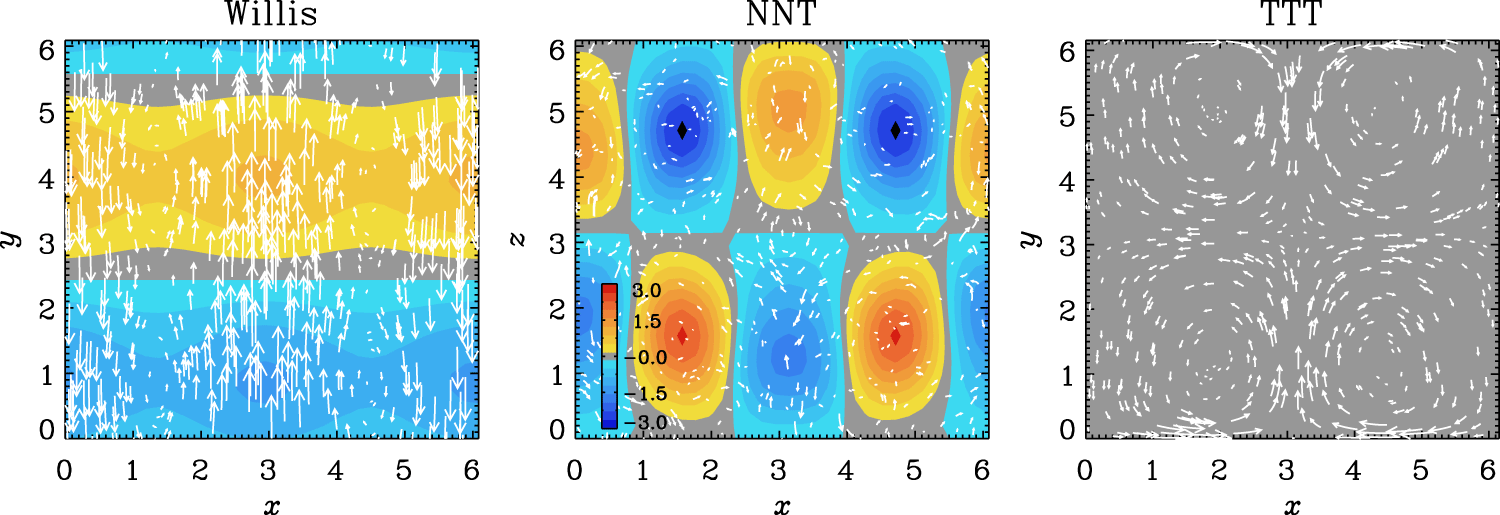
Figure 7. Column averages of the magnetic fields for the Willis, NTT and TTT dynamos. Similarly to figure 4 for the mean velocity, the mean magnetic field in the plane is indicated by vectors together with the normal component colour coded. The normal component is normalized by the r.m.s. value of this mean field based on all three components.
For the 15 % supercritical TTT flow, on the other hand, the actual magnetic field is growing, but the  $xy$ average remains small. This does not necessarily imply that there is no mean field. Indeed, a finite mean field is, in this case, obtained by taking column averages just over the $z$ direction. This is shown in figure 7, where we compare the resulting column averages of the magnetic fields for the Willis, NTT and TTT dynamos. We see that, even though we found a clear mean field for the Willis flow through planar averaging, we also find a clear mean field from just averaging over the $z$ direction. Indeed, by computing the ratio of the r.m.s. values of the column averaged mean field and the total field, $q=\overline{B}_{\text{rms}}/B_{\text{rms}}$, we now find the value 0.81 for the Willis dynamo, 0.08 for the NNT dynamo and 0.45 for the TTT dynamo. The latter value was already indicated in table 1 with an asterisk. The fact that the value for the NNT flow is small suggests that the flow does not have an important column average and that the appropriate average is here indeed the $xy$ average.
It is important to emphasize that the Willis dynamo is completely isotropic with respect to the  $x$,
$x$,  $y$ and $z$ directions. Therefore, all three planar averages give equally strong mean fields in this linear dynamo problem. In figure 2, we plotted $\overline{B}_{x}(z_{\ast })$, but this cannot be the same mean field seen for the Willis dynamo in figure 7, which is instead a field $\overline{B}_{y}(x)$ that is obtained through $yz$ averaging. The third component, $\overline{B}_{z}(y)$, is also excited and can be seen through $xz$ averaging. It is only in the nonlinear case that one of the three planar averages will survive, as has been demonstrated in connection with helical isotropic turbulence; see figure 6 of Brandenburg (Reference Brandenburg2001). The other two planar averages begin to decay in the nonlinear regime.

Figure 8. Dependence of the real and imaginary parts of  $\tilde{\unicode[STIX]{x1D702}}_{ij}$ on $\unicode[STIX]{x1D714}$ for the Willis flow in the marginally exited case with $\unicode[STIX]{x1D702}=0.403$ and for $k=1$. The off-diagonal components vanish, $\text{Re}\,\tilde{\unicode[STIX]{x1D702}}_{xx}$ (blue) is always positive, $\text{Im}\,\tilde{\unicode[STIX]{x1D702}}_{xx}$ (black) is always negative and $\tilde{\unicode[STIX]{x1D702}}_{yy}$ (red) changes sign from negative to positive values as $\unicode[STIX]{x1D714}$ increases. The dotted lines give approximate fits: $\tilde{\unicode[STIX]{x1D702}}_{xx}\approx 0.295/(1+2\text{i}\unicode[STIX]{x1D714})$ and $\tilde{\unicode[STIX]{x1D702}}_{yy}\approx 0.13[-1+(4\unicode[STIX]{x1D714})^{2}]/[1+(3\unicode[STIX]{x1D714})^{2}+(1.6\unicode[STIX]{x1D714})^{4}]$.
Based on the analysis of the time series of the components of the magnetic field, we find mean-field dynamo action for the NNT and TTT cases. However, we still cannot say much more about the nature of the dynamo action. To make further progress, we now use the TFM to determine the underlying mean-field transport coefficients. Their knowledge would allow us to model the generation of mean magnetic fields and thereby to characterize the nature of the dynamo process. This is discussed in the next section.
6 Test-field results for the different dynamos
6.1 Results for the Willis flow
We begin by showing in figure 8 the dependence of  $\tilde{\unicode[STIX]{x1D702}}_{ij}$ on $\unicode[STIX]{x1D714}$ for $k=1$. We recall that $k=1$ corresponds to the lowest wavenumber within our domain of size $2\unicode[STIX]{x03C0}$. We see that $\tilde{\unicode[STIX]{x1D702}}_{xx}$ and $\tilde{\unicode[STIX]{x1D702}}_{yy}$ have non-vanishing real parts at $\unicode[STIX]{x1D714}=0$. Furthermore, $\text{Re}\,\tilde{\unicode[STIX]{x1D702}}_{xx}$ is always positive and approaches zero monotonically. By contrast, $\text{Re}\,\tilde{\unicode[STIX]{x1D702}}_{yy}$ is negative, but grows and crosses zero at $\unicode[STIX]{x1D714}=0.3$, reaches a maximum at $\unicode[STIX]{x1D714}=0.7$ and then falls off toward zero.
For  $\unicode[STIX]{x1D714}\neq 0$, $\tilde{\unicode[STIX]{x1D702}}_{xx}$ becomes complex while $\tilde{\unicode[STIX]{x1D702}}_{yy}$ remains real. The $\tilde{\unicode[STIX]{x1D702}}_{xx}$ component determines the evolution of $\overline{A}_{x}$ and correspondingly $\overline{B}_{y}$, which is decaying even in the marginally excited case; see figure 2. The time dependence of $\overline{\boldsymbol{B}}$ leads a memory effect in the evolution of $\overline{A}_{x}$, i.e. to a frequency-dependent time delay in the electromotive force (Hubbard & Brandenburg Reference Hubbard and Brandenburg2009). By contrast, $\tilde{\unicode[STIX]{x1D702}}_{yy}$ is real for time-independent mean magnetic fields, but it is negative for $\unicode[STIX]{x1D714}\rightarrow 0$ and $k\rightarrow 0$; see figure 9. However, $\tilde{\unicode[STIX]{x1D702}}_{yy}$ is not sufficiently negative to overcome diffusive decay, because $\unicode[STIX]{x1D702}+\tilde{\unicode[STIX]{x1D702}}_{yy}$ is still positive. This is surprising, but we have to realize that $\tilde{\unicode[STIX]{x1D702}}_{yy}$ depends also on $z$; see figure 10.

Figure 9. Dependence of  $\tilde{\unicode[STIX]{x1D702}}_{xx}$ (red) and $\tilde{\unicode[STIX]{x1D702}}_{yy}$ (blue) on $k$ for the Willis flow in the marginally exited case with $\unicode[STIX]{x1D702}=0.403$ and for $\unicode[STIX]{x1D714}=0$. The dashed line denotes the fit $-0.233+0.11k^{2}$ and will be discussed in § 7.2.

Figure 10. Dependence of  $\tilde{\unicode[STIX]{x1D702}}_{xx}(z)$ (blue) and $\tilde{\unicode[STIX]{x1D702}}_{yy}(z)$ (red) on $z$ for the Willis flow in the marginally exited case with $\unicode[STIX]{x1D702}=0.4031$, $k=1$ and $\unicode[STIX]{x1D714}=0$.
In figure 11 we plot the local minima, maxima and averages of  $\tilde{\unicode[STIX]{x1D702}}_{xx}$ and $\tilde{\unicode[STIX]{x1D702}}_{yy}$ versus $\unicode[STIX]{x1D702}$. Those $z$ averages are denoted by an overbar. We see that the onset of dynamo action ( $\unicode[STIX]{x1D702}=\unicode[STIX]{x1D702}_{\text{crit}}\approx 0.403$) coincides with the point where $\unicode[STIX]{x1D702}+\tilde{\unicode[STIX]{x1D702}}_{yy}^{\text{min}}=0$. Interestingly, it is apparently not the spatial average of $\tilde{\unicode[STIX]{x1D702}}_{yy}(z)$ which must become negative for instability, but the minimum of $\tilde{\unicode[STIX]{x1D702}}_{yy}(z)$.

Figure 11. Dependence of  $\tilde{\unicode[STIX]{x1D702}}_{xx}$ (blue) and $\tilde{\unicode[STIX]{x1D702}}_{yy}$ (red) on $\unicode[STIX]{x1D702}$ for the Willis flow using $k=1$ and $\unicode[STIX]{x1D714}=0$. The values of the minima and maxima of $\tilde{\unicode[STIX]{x1D702}}_{xx}$ and $\tilde{\unicode[STIX]{x1D702}}_{yy}$ are shown as dotted lines. Their $z$ averages are denoted by an overbar and are also plotted for comparison. The value of $-\unicode[STIX]{x1D702}$ is overplotted as a solid line to show that $\unicode[STIX]{x1D702}+\tilde{\unicode[STIX]{x1D702}}_{yy}^{\text{min}}=0$ when $\unicode[STIX]{x1D702}\approx 0.403$.
6.2 Results for the NNT and TTT flows
For the NNT flow, the resulting profiles for the components of the turbulent magnetic diffusivity are shown in figure 12. We see that both  $\tilde{\unicode[STIX]{x1D702}}_{xx}$ and $\tilde{\unicode[STIX]{x1D702}}_{yy}$ become negative, but not quite as much as to make the sum of $\unicode[STIX]{x1D702}+\tilde{\unicode[STIX]{x1D702}}_{ij}$ negative. Nevertheless, it is still likely that this mean-field dynamo is due to the negative turbulent magnetic diffusivity, because the full system is more complicated due to the presence of pumping effects and the non-locality in space, for example.
For the TTT case, mean-field dynamo action has only been obtained for column averaged fields. Applying the TFM for  $xy$ averages, we find that the only non-vanishing components of the eight transport coefficients are $\tilde{\unicode[STIX]{x1D702}}_{xx}$ and $\tilde{\unicode[STIX]{x1D702}}_{yy}$. Both are positive, so no mean-field dynamo action can be expected for $xy$ planar averages. As we have seen above, the appropriate average is the column average. This case is more complicated and involves altogether 27 turbulent transport coefficients; see also Warnecke et al. (Reference Warnecke, Rheinhardt, Käpylä, Käpylä and Brandenburg2018) for a recent study in spherical coordinates, where longitudinal averages were used. We will not consider this case here, but adopt instead $xy$ and $xz$ averages, as was done by Andrievsky (Reference Andrievsky2015) in the investigation of the Taylor–Green flow, where mean fields were also only found through column averaging. They confirmed the presence of negative turbulent magnetic diffusivity for this flow, which was first found by Lanotte et al. (Reference Lanotte, Noullez, Vergassola and Wirth1999) and was not seen when using just planar averages (Devlen et al. Reference Devlen, Brandenburg and Mitra2013).

Figure 12. Dependence of  $\tilde{\unicode[STIX]{x1D702}}_{xx}$ (blue) and $\tilde{\unicode[STIX]{x1D702}}_{zz}$ (red) on $y$ for the NNT flow with $\unicode[STIX]{x1D702}=0.133$, $k=1$ and $\unicode[STIX]{x1D714}=0$.
In figures figure 13(a) and 13(b), we show the results for the TTT flow as functions of  $x$ and $y$, respectively. Note that both $\tilde{\unicode[STIX]{x1D702}}_{zz}(x)$ and $\tilde{\unicode[STIX]{x1D702}}_{zz}(y)$ are negative over extended ranges. The sum $\unicode[STIX]{x1D702}+\tilde{\unicode[STIX]{x1D702}}_{zz}$ is still positive, but we have to remember that the mean-field dynamo works in this case with $z$ averages, so the $yz$ and $xz$ averages adopted here are prone to additional cancellation. This suggests that the mean-field generation in this case is indeed of the type of a negative turbulent diffusivity dynamo.

Figure 13. Dependence of  $\tilde{\unicode[STIX]{x1D702}}_{ij}$ on (a) $x$ (for $yz$ averages) and on (b) $y$ (for $xz$ averages) for the TTT flow with $k=1$ and $\unicode[STIX]{x1D714}=0$ in a domain of size $(2\unicode[STIX]{x03C0})^{3}$ using $\unicode[STIX]{x1D702}=0.083$.
As we will show next, for the  $\unicode[STIX]{x03C0}^{3}$ domain, we always find a non-vanishing average, but it may not be a mean-field dynamo, because the scales of averaging and of the fluctuations are very similar. To get an idea about the resulting mean-field transport coefficients, we now solve the test-field equations in a $\unicode[STIX]{x03C0}^{3}$ domain using the standard TFM for the NNT and TTT flows. However, given that the Reynolds rules do not apply here, the TFM results cannot be fully reliable.

Figure 14. Dependences of  $\tilde{\unicode[STIX]{x1D6FC}}_{ij}$ and $\tilde{\unicode[STIX]{x1D702}}_{ij}$ on $y$ for the NNT flow with $k=1$ and $\unicode[STIX]{x1D714}=0$ in a $\unicode[STIX]{x03C0}^{3}$ domain using $\unicode[STIX]{x1D702}=0.133$. For the diagonal components, we show the sum $\unicode[STIX]{x1D702}+\tilde{\unicode[STIX]{x1D702}}_{ii}$. The dotted lines denote the result using averaging over a $(2\unicode[STIX]{x03C0})^{2}$ plane.

Figure 15. Similar to figure 14, but for the TTT flow using  $\unicode[STIX]{x1D702}=0.083$.
In figures 14 and 15 we show test-field results for the NNT and TTT cases in  $\unicode[STIX]{x03C0}^{3}$ domains using the appropriate lateral and vertical boundary conditions. For both flows, we also have done calculations in domains where the extent in the $y$ or $z$ directions for the NNT and TTT flows, respectively, is from 0 to $2\unicode[STIX]{x03C0}$. The only difference to the shorter domain is that all four components of $\tilde{\unicode[STIX]{x1D6FC}}_{ij}$ are antisymmetric around the middle point of the $[0,2\unicode[STIX]{x03C0}]$ domain, while all four components of $\tilde{\unicode[STIX]{x1D702}}_{ij}$ are symmetric. Here we only show the results in the range $0\leqslant y\leqslant \unicode[STIX]{x03C0}$ for the NNT flow and in the range $0\leqslant z\leqslant \unicode[STIX]{x03C0}$ for the TTT flow.
We also compare with solutions over the full  $(2\unicode[STIX]{x03C0})^{2}$ cross-section. The actual solutions for the response to the test fields are then unchanged, but now the planar averages extend over the full $(2\unicode[STIX]{x03C0})^{2}$ plane, so there can be complete cancellation for certain variables – notably the two components of $\tilde{\unicode[STIX]{x1D6FC}}_{ij}$ for $i=j$, as well as for the two components of $\tilde{\unicode[STIX]{x1D702}}_{ij}$ for $i\neq j$.
7 Comparison with mean-field dynamos
7.1 The absence of  $\unicode[STIX]{x1D6FC}$ effect

We now discuss in more detail the possibility of mean-field dynamo action based on the present results. Given that the diagonal components of  $\unicode[STIX]{x1D6FC}_{ij}$ are finite, there is the possibility of $\unicode[STIX]{x1D6FC}^{2}$ dynamo action, except that the values of $\unicode[STIX]{x1D6FC}$ appear too small in the sense that the dynamo number, $|\langle \unicode[STIX]{x1D6FC}\rangle |/\langle \unicode[STIX]{x1D702}+\unicode[STIX]{x1D702}_{\text{t}}\rangle k_{1}$, is below the estimated critical value of unity. Here, $\unicode[STIX]{x1D702}_{\text{t}}$ is the average of the two diagonal components of the magnetic diffusivity tensor. Furthermore, given that the off-diagonal components of $\tilde{\unicode[STIX]{x1D702}}_{ij}$ are finite, there could be a Rädler effect, also known at $\unicode[STIX]{x1D734}\times \overline{\boldsymbol{J}}$ effect, because the off-diagonal components of $\tilde{\unicode[STIX]{x1D702}}_{ij}$ contribute to a term in the mean electromotive force of the form $\overline{\boldsymbol{{\mathcal{E}}}}=\cdots +\unicode[STIX]{x1D739}\times \overline{\boldsymbol{J}}$, where $\unicode[STIX]{x1D739}$ is often also aligned with the axis of rotation, $\unicode[STIX]{x1D734}$. For our planar averages, its components are given by $\unicode[STIX]{x1D6FF}_{i}=-\textstyle \frac{1}{2}\unicode[STIX]{x1D716}_{ijk}\unicode[STIX]{x1D702}_{jk}$.
A well-known problem with this latter idea, however, is that the Rädler effect alone cannot explain an increase of the magnetic energy of the mean field. It can only work in conjunction with other effects such as shear. In the presence of an  $\unicode[STIX]{x1D6FC}$ effect, it can also make the solutions oscillatory and cause migratory dynamo waves, which becomes more pronounced in a periodic domain, as can be seen by solving the corresponding eigenvalue problem.
In the present case, we need to address the questions whether, first, the  $\unicode[STIX]{x1D6FC}$ effect is strong enough to produce $\unicode[STIX]{x1D6FC}^{2}$ or $\unicode[STIX]{x1D6FC}$–shear ( $\unicode[STIX]{x1D6FC}\unicode[STIX]{x1D6FA}$) dynamo action, depending on whether or not the mean flow plays a role, and second, whether the Rädler effect plays a role, possibly in conjunction with effects other than the mean flow, for example the $\unicode[STIX]{x1D6FC}$ effect. The first point, in fact, was already discussed by Andrievsky (Reference Andrievsky2015). Assuming the total magnetic field can be written as a series expansion
 $$\begin{eqnarray}\boldsymbol{B}=\mathop{\sum }_{n=0}^{\infty }\boldsymbol{b}_{n}\unicode[STIX]{x1D716}^{n},\end{eqnarray}$$
 where  $\unicode[STIX]{x1D716}$ is a small scaling factor that relates the slow-changing spatial variables to the fast-changing ones. The $\unicode[STIX]{x1D6FC}$ effect can be written as an eigenvalue problem for the leading term $\boldsymbol{b}_{0}$
 $$\begin{eqnarray}\unicode[STIX]{x1D735}\times \unicode[STIX]{x1D736}\boldsymbol{b}_{0}=\unicode[STIX]{x1D6EC}_{0}\boldsymbol{b}_{0},\end{eqnarray}$$
 where  $\unicode[STIX]{x1D6EC}_{0}$ is the eigenvalue, $\unicode[STIX]{x1D736}$ is a tensor, $\langle \boldsymbol{U}\times \boldsymbol{S}_{i}\rangle$ is the $i$th column of $\unicode[STIX]{x1D736}$, $\boldsymbol{U}$ is the flow field, $\boldsymbol{S}_{i}$ is the solution of
 $$\begin{eqnarray}{\mathcal{I}}\boldsymbol{S}_{i}=-\frac{\unicode[STIX]{x2202}\boldsymbol{U}}{\unicode[STIX]{x2202}x_{i}},\end{eqnarray}$$
 and  ${\mathcal{I}}$ is the induction operator,
 $$\begin{eqnarray}{\mathcal{I}}\boldsymbol{b}_{0}=\unicode[STIX]{x1D735}\times (\boldsymbol{U}\times \boldsymbol{b}_{0})+\unicode[STIX]{x1D702}\unicode[STIX]{x1D6FB}^{2}\boldsymbol{b}_{0}.\end{eqnarray}$$
If the flow is parity invariant,
 $$\begin{eqnarray}\boldsymbol{U}(-\boldsymbol{x})=-\boldsymbol{U}(\boldsymbol{x}),\end{eqnarray}$$
 then  $\boldsymbol{S}_{i}$ must be anti-invariant, so the operator of the $\unicode[STIX]{x1D6FC}$ effect is $\unicode[STIX]{x1D736}=0$. From (3.6) and (3.9), we see that the three optimal flows are all parity invariant in the full $(2\unicode[STIX]{x03C0})^{3}$ domain, hence no $\unicode[STIX]{x1D6FC}$ effect is expected at the leading order.
7.2 The negative turbulent magnetic diffusivity dynamo
To model a negative turbulent magnetic diffusivity dynamo, we must take care of the fact that the high wavenumbers are not being destabilized at the same time. As we have seen from figure 9,  $\unicode[STIX]{x1D702}_{\text{t}}$ is negative only for $k\lesssim 1.5$. A simple way of taking the $k$ dependence of the turbulent magnetic diffusivity into account is to expand $\tilde{\unicode[STIX]{x1D702}}_{yy}(k)$ up to the next order in the diffusive effects (which are even in $k$), i.e.
 $$\begin{eqnarray}\tilde{\unicode[STIX]{x1D702}}_{yy}(k)=\tilde{\unicode[STIX]{x1D702}}_{yy}^{(0)}+\tilde{\unicode[STIX]{x1D702}}_{yy}^{(2)}k^{2}+\cdots .\end{eqnarray}$$
 Looking at figure 9 for the Willis flow, we see that in the proximity of  $k=1$, which corresponds to the largest scale in the computational domain of $2\unicode[STIX]{x03C0}$, the $k$-dependence of $\tilde{\unicode[STIX]{x1D702}}_{yy}(k)$ can well be described by the parameters $\tilde{\unicode[STIX]{x1D702}}_{yy}^{(0)}\approx -0.233$ and $\tilde{\unicode[STIX]{x1D702}}_{yy}^{(2)}\approx 0.11$. In addition, there is still the microphysical magnetic diffusivity, which is positive ( $\unicode[STIX]{x1D702}=0.403$). The mean-field equations for the magnetic field components decouple. For the purpose of this problem, we just need to consider the equation for $\overline{A}_{y}$, which can then be written as
 $$\begin{eqnarray}\frac{\unicode[STIX]{x2202}\overline{A}_{y}}{\unicode[STIX]{x2202}t}=[\unicode[STIX]{x1D702}+\tilde{\unicode[STIX]{x1D702}}_{yy}^{(0)}]\frac{\unicode[STIX]{x2202}^{2}\overline{A}_{y}}{\unicode[STIX]{x2202}z^{2}}-\tilde{\unicode[STIX]{x1D702}}_{yy}^{(2)}\frac{\unicode[STIX]{x2202}^{4}\overline{A}_{y}}{\unicode[STIX]{x2202}z^{4}}.\end{eqnarray}$$
 Note that the minus sign in front of the fourth derivative corresponds to positive diffusion if  $\tilde{\unicode[STIX]{x1D702}}_{yy}^{(2)}$ is positive, and so does the plus sign in front of the second derivative, unless the term in squared brackets is negative, which is the case we are considering here.
We have seen from figure 10 that  $\unicode[STIX]{x1D702}+\tilde{\unicode[STIX]{x1D702}}_{yy}$ just barely approaches zero and does not become negative. This is unexpected. To understand the problem, we now solve (7.7) numerically with an assumed amplitude for the variation of $\tilde{\unicode[STIX]{x1D702}}_{yy}^{(0)}$ of the form
 $$\begin{eqnarray}\tilde{\unicode[STIX]{x1D702}}_{yy}^{(0)}=\overline{\unicode[STIX]{x1D702}}_{yy}^{(0)}(1+\unicode[STIX]{x1D716}\cos 2z),\end{eqnarray}$$
 where  $\unicode[STIX]{x1D716}$ quantifies the amplitude of the spatial variation around the average value, which is $\overline{\unicode[STIX]{x1D702}}_{yy}^{(0)}$. It turns out that, with the parameters given in figure 9, and $\unicode[STIX]{x1D702}=0.403$ for the microphysical magnetic diffusivity, marginally excited solutions are only possible when $\unicode[STIX]{x1D716}>1.99$. On the other hand, when trying to fit the functional form of $\tilde{\unicode[STIX]{x1D702}}_{yy}^{(0)}$ in figure 10, it turns out that it is possible with $\unicode[STIX]{x1D716}=1.99$, but only if $\overline{\unicode[STIX]{x1D702}}_{yy}^{(0)}=-0.133$ instead of $-0.233$, as expected from the fit to the $k$ dependence.
It is not entirely clear how to interpret these findings. We do not know enough about such dynamos whose parameters depend both on  $z$ and $k$ at the same time. Nevertheless, it seems that the overall idea of a negative turbulent magnetic diffusivity dynamo is the right one, but that the correct description is more complicated than what is suggested by (7.7). Effects such as pumping and additional non-localities have been ignored.
7.3 Mean-field excitation conditions for the NNT and TTT cases
To address the possibility of dynamo action from the  $\unicode[STIX]{x1D6FC}$ and Rädler effects, we use the profiles of $\tilde{\unicode[STIX]{x1D6FC}}_{ij}(z)$ and $\tilde{\unicode[STIX]{x1D702}}_{ij}(z)$, as obtained from the TFM. To get an idea of how close to the dynamo onset we are, we scale the dynamo active coefficients by an amplitude factor, i.e. $\tilde{\unicode[STIX]{x1D6FC}}_{ij}\rightarrow \tilde{\unicode[STIX]{x1D6FC}}_{ij}A_{\unicode[STIX]{x1D6FC}}$ for $i=j$, and $\tilde{\unicode[STIX]{x1D702}}_{ij}\rightarrow \tilde{\unicode[STIX]{x1D702}}_{ij}A_{\unicode[STIX]{x1D6FF}}$ for $i\neq j$. We then choose a value of $A_{\unicode[STIX]{x1D6FF}}$ and determine the critical values of $A_{\unicode[STIX]{x1D6FC}}$ above which there is dynamo action, i.e. a growing solution. All solutions are oscillatory and correspond to standing waves. The result is shown in table 2.
Table 2. Critical values of  $A_{\unicode[STIX]{x1D6FC}}$ and the corresponding frequencies $\text{Im}\,\unicode[STIX]{x1D706}$ for different values of $A_{\unicode[STIX]{x1D6FF}}$ for the NNT and TTT dynamos. The type of averaging employed for obtaining the mean-field coefficients is listed under ‘aver’ ( $xy$ or $xz$). All solutions are standing waves.

We see that for the NNT flow,  $A_{\unicode[STIX]{x1D6FC}}$ decreases with increasing values of $A_{\unicode[STIX]{x1D6FF}}\leqslant 5$, so the dynamo becomes slightly easier to excite. For $A_{\unicode[STIX]{x1D6FF}}=10$, however, $A_{\unicode[STIX]{x1D6FC}}$ increases again. The oscillation frequency increases slightly as $A_{\unicode[STIX]{x1D6FF}}$ increases. For the TTT model, on the other hand, $A_{\unicode[STIX]{x1D6FC}}$ always increases with $A_{\unicode[STIX]{x1D6FF}}$, i.e. the $\unicode[STIX]{x1D6FF}$ effect does not contribute to dynamo dynamo action, but suppresses it. In both cases, the values of $A_{\unicode[STIX]{x1D6FC}}$ are small unless the scaling factor $A_{\unicode[STIX]{x1D6FF}}$ is at least $O(10)$.
8 Discussion and conclusions
There is only a small number of successful experimental dynamos to date (Gailitis et al. Reference Gailitis, Lielausis, Dementév, Platacis, Cifersons, Gerbeth, Gundrum, Stefani, Christen and Hänel2000; Stieglitz & Müller Reference Stieglitz and Müller2001; Monchaux et al. Reference Monchaux, Berhanu, Bourgoin, Moulin, Odier, Pinton, Volk, Fauve, Mordant and Petrelis2007). Several other dynamo experiments are currently in operation; see the review by Adams et al. (Reference Adams, Stone, Zimmerman and Lathrop2015), who also discuss the newer Madison dynamo experiment and the Derviche–Tourneur sodium experiment. They all work with liquid sodium, and they all involve flows with significant swirl – in anticipation that those types of dynamos would be most suitable for driving dynamo action most easily. Different classes of optimal dynamos display flows largely reminiscent of those with an  $\unicode[STIX]{x1D6FC}$ effect, so it was natural to ask whether such an effect played a role in generating the magnetic field in those cases. It now turns out that this does not have to be the case. Instead, the optimal dynamo of Willis (Reference Willis2012) is driven by a negative turbulent magnetic diffusivity. This was rather unexpected, because such dynamos are not very common and have not been studied much (Zheligovsky, Podvigina & Frisch Reference Zheligovsky, Podvigina and Frisch2001; Zheligovsky Reference Zheligovsky2012; Devlen et al. Reference Devlen, Brandenburg and Mitra2013).
The concept of negative turbulent magnetic diffusivity is somewhat mysterious and may have seemed to be more like a qualitative excuse for lack of a more definitive term than a quantitative and rigorous statement. In fact, we are not aware of a quantitative mean-field model employing negative magnetic diffusivity until now. This would need to be done with sufficient care to prevent small-scale instabilities. Here we have presented such a model that is stabilized by the inclusion of hyperdiffusivity. In the parameter regime of interest, it turned out that the sign of the coefficient of hyperdiffusivity is indeed such that it has a stabilizing effect. Among the systems with negative diffusivity and a stabilizing hyperdiffusivity is the Kuramoto–Sivashinsky equation, which has been employed as a model of forest fires (Hyman & Nicolaensko Reference Hyman and Nicolaensko1986). In that case, however, there is also an advection term, making the system nonlinear, and also the system size was large compared to the typical size of structures. This led to a rich spatio-temporal evolution. It is therefore of interest to ask whether such dynamics could possibly also be realized in an experimental or at least a numerical dynamo set-up.
Similarly to the Willis dynamo, the NNT dynamo also exhibits negative turbulent magnetic diffusivity. However, unlike the Willis dynamo, it is not isotropic and exists only for one of the three possible planar averages. Finally, the TTT dynamo shows no mean field after planar averaging. Nevertheless, a mean field exists also in this case, but it requires column averaging over only one coordinate direction. It is similar to the Taylor–Green flow, for which Lanotte et al. (Reference Lanotte, Noullez, Vergassola and Wirth1999) also found negative turbulent magnetic diffusivity, and the corresponding mean field can only be found through column averaging (Andrievsky Reference Andrievsky2015). Note that both NNT and TTT flows can be transformed into to a general Taylor–Green flow by a shift of  $\unicode[STIX]{x03C0}/2$ in each direction. The spatial averaging then depends on the specific combination of field coefficients.
To assess the possibility of  $\unicode[STIX]{x1D6FC}$ or $\unicode[STIX]{x1D6FF}$ effect dynamos action in $\unicode[STIX]{x03C0}^{3}$ subdomains, we have compared with the corresponding mean-field dynamos. It turned out that both are strongly subcritical and would only become marginally excited when either the $\unicode[STIX]{x1D6FC}$ effect or the $\unicode[STIX]{x1D6FF}$ effect are scaled up by factors between five and ten. These factors seem rather large, making a mean-field interpretation based on the $\unicode[STIX]{x1D6FC}$ and $\unicode[STIX]{x1D6FF}$ effects in these cases unlikely. Thus, it now seems that the class of dynamos based on negative turbulent magnetic diffusivity is broader than previously anticipated and may include the class of optimal dynamos as well.
Acknowledgements
We thank the anonymous reviewers and P. Livermore for their useful comments and M. Käpylä, A. Pevtsov, I. Virtanen and N. Yokoi for providing a splendid atmosphere at the Nordita-supported program on Solar Helicities in Theory and Observations. We would like to also thank W. Herreman for insightful discussions regarding the mean-field theory. This research was supported in part by the NSF Astronomy and Astrophysics Grants Program (grant 1615100), the University of Colorado through its support of the George Ellery Hale visiting faculty appointment, and the Leverhulme Trust grant PRG-2017-169. We acknowledge the allocation of computing resources provided by the Swedish National Allocations Committee at the Center for Parallel Computers at the Royal Institute of Technology in Stockholm.


 Open access