


1. Introduction
Flows featuring gas–liquid interfaces abound in all areas of fluid dynamics. When the effects of impurities are neglected, the dynamics of these interfacial flows is reasonably well understood. For low enough Froude numbers, the interface is flat. While the usual no-slip condition holds near solid boundaries, for negligible gas viscosity, the dynamics at the gas–liquid interface is usually modelled using a simple stress-free condition along a non-deformable surface. This ‘stress-free’ interface condition expresses the nullity of the gradient of the tangential velocity in the direction normal to the interface, whereas a no-slip condition expresses the nullity of the velocity relative to the interface. Once the boundary conditions are well chosen, solutions to the governing equations can be sought either analytically or numerically.
This simple approach breaks down however in practice when the working fluid is standard or demineralised water, as opposed to e.g. castor oil (Batchelor Reference Batchelor2000). The (unavoidable) presence of dust implies particles of various sizes adhere to the interface via multiple forces such as van der Waals interactions, covalent bonds, dipolar interactions and so forth. As it stands, for relatively low pollutant concentrations, a monomolecular layer of particles forms by adsorption at the interface (Scriven Reference Scriven1960; Bernal et al. Reference Bernal, Hirsa, Kwon and Willmarth1989; Lopez & Hirsa Reference Lopez and Hirsa1998; Ponce-Torres & Vega Reference Ponce-Torres and Vega2016). The surface tension is locally lower where the pollutants are present, which induces a heterogeneous distribution of surface tension and hence tangential Marangoni stresses. This effect has been reported in various interfacial flows including bubbles (see e.g. Batchelor Reference Batchelor2000 or Magnaudet & Eames Reference Magnaudet and Eames2000) and Faraday experiments (Martín & Vega Reference Martín and Vega2006). It is traditionally modelled using boundary conditions that rely on a closure between the local concentration  $c$ and the surface tension $\sigma$. Such models where $\sigma =f(c)$ imply the calibration of many constants, some of them possibly time-dependent (Ponce-Torres & Vega Reference Ponce-Torres and Vega2016), whereas the real chemical composition and even the concentration of the pollutants are rarely known in detail. A really simple phenomenological model is therefore called for to address most polluted interfaces at once, irrespective of their exact composition and properties. The goal of this paper, by considering a simple enough flow prototype, is to introduce and validate such a phenomenological model by comparing its numerical prediction to experimental results.
In this work, the free-surface flow spinning above a rotating disc is considered at low rotation rates. The cylindrical sidewall is held at rest. This flow is characterised geometrically by the aspect ratio  $G=H/R$, where $H$ is the undisturbed fluid height and $R$ the interior radius, and dynamically by a Reynolds number $Re=\rho \varOmega R^2/\mu$ based on the rotation rate $\varOmega$, the liquid density $\rho$ and the dynamic viscosity $\mu$ (Hyun Reference Hyun1985; Spohn & Daube Reference Spohn and Daube1991; Spohn, Mory & Hopfinger Reference Spohn, Mory and Hopfinger1993; Lopez Reference Lopez1995; Iwatsu Reference Iwatsu2004, Reference Iwatsu2005; Piva & Meiburg Reference Piva and Meiburg2005; Bouffanais & Lo Jacono Reference Bouffanais and Lo Jacono2009; Cogan, Ryan & Sheard Reference Cogan, Ryan and Sheard2011). The comparison performed by Spohn & Daube (Reference Spohn and Daube1991) between experimental and computational velocity profiles obtained using the free-slip boundary condition has revealed that for $G=7/4$, there is a mismatch in the tangential velocity profiles especially near the liquid–air interface. The value of $G$ that caught our attention is $G=1/4$. In this geometry, a mode $m=3$ (where $m$ is the dominant azimuthal wavenumber) was identified experimentally as the first instability encountered when increasing $Re$ (Miraghaie, Lopez & Hirsa Reference Miraghaie, Lopez and Hirsa2003; Lopez et al. Reference Lopez, Marques, Hirsa and Miraghaie2004). Numerical simulations were also reported in the same papers and summarised recently by Hirsa & Lopez (Reference Hirsa and Lopez2021). A mode $m=3$ was also reported in this study as the most unstable mode. The numerical domain used consisted however of two mirror-concatenated copies of the original domain, which has the unphysical property of allowing for mass transfer through the mid-plane representing the interface. To our knowledge, no simulation of the original geometry has been reported using stress-free boundary conditions until the recent study of Faugaret (Reference Faugaret2020). In that study, linear stability analysis based on the stress-free boundary condition leads to a modal selection at odds with the experimental results reported earlier: the first unstable mode occurs at higher $Re$ than in the experiment and has the symmetry $m=2$ rather than $m=3$. Thus $G=1/4$ appears particularly demanding from a bifurcation point of view and represents an interesting test for a modelling strategy.
The first investigations to blame the presence of surfactant-like pollutants for the observed mismatch were performed by Spohn & Daube (Reference Spohn and Daube1991), as well as Lopez, Hirsa and co-authors (Lopez & Chen Reference Lopez and Chen1998; Lopez & Hirsa Reference Lopez and Hirsa1998). A numerical investigation of the same system with  $G=1/4$ was conducted by Kwan, Park & Shen (Reference Kwan, Park and Shen2010) by assuming a finite concentration of a given surfactant at the interface rather than using a stress-free boundary condition. A parabolic closure was used to link the surface tension to the superficial concentration field. This work is useful as a confirmation of the modal instability observed in experiments, yet it does not contain any parametric study nor any bifurcation diagram. In general, the stability threshold values found in experiments match those predicted in numerics using free-slip conditions, provided the aspect ratio $G$ is large enough, as in the case where $G=2$ (Lopez et al. Reference Lopez, Marques, Hirsa and Miraghaie2004; Serre & Bontoux Reference Serre and Bontoux2007; Cogan et al. Reference Cogan, Ryan and Sheard2011; Faugaret Reference Faugaret2020). The situation is entirely different for values of $G$ below unity. In a recent publication, Faugaret et al. (Reference Faugaret, Duguet, Fraigneau and Martin Witkowski2020) carried out a joint experimental/numerical study of the same flow for a smaller aspect ratio $G=1/14$. This aspect ratio is characterised by a much greater mismatch between thresholds in $Re$ (Poncet & Chauve Reference Poncet and Chauve2007; Kahouadji, Martin Witkowski & Le Quéré Reference Kahouadji, Martin Witkowski and Le Quéré2010). A simple surfactant-free model, initially suggested by Spohn & Daube (Reference Spohn and Daube1991), was found to lower significantly the stability threshold $Re_c$ without fully resolving the mismatch. In this model, the radial velocity $u_r$ is assumed to be zero over the entire interface, whereas the azimuthal component only has zero normal derivative. This approximation is known in other (often two-dimensional) flow conditions as the ‘stagnant cap approximation’. We do not use this denomination to emphasize that the condition holds here on the radial component only. At the very end of the paper by Faugaret et al. (Reference Faugaret, Duguet, Fraigneau and Martin Witkowski2020), a ‘mixed model’, intermediate between the stress-free and the Spohn–Daube model, was suggested. It was analysed using linear stability theory only. The values of $Re_c$ associated with this model are quantitatively much closer to the experimental thresholds. This suggests a deeper analysis of the model using a fully nonlinear methodology. The goal of the present investigation is first to justify the model based on a new experimental campaign, then assess its ability to reproduce the experimental dynamics qualitatively and quantitatively. The present study relies on an experimental set-up, a linear stability solver and a direct numerical simulation code with the mixed boundary condition implemented. This new study departs from the former numerical investigation of Faugaret (Reference Faugaret2020) and Faugaret et al. (Reference Faugaret, Duguet, Fraigneau and Martin Witkowski2020) by the use of fully nonlinear simulations as well as the different physics associated with another value of $G$.
$G$.
The plan of the paper is as follows: § 2 contains a description of the tools used in the whole study. In § 3, the validity of the stress-free boundary conditions is questioned in light of a new Lagrangian tracking experiment. The model is introduced both in stationary and non-stationary flow conditions. The joint experimental/computational analysis of the bifurcations resulting from the modified base flow is reported in § 4 before the conclusions in § 5. The numerical methods and their validation are explained in the Appendices A and B, while Appendix C details both experimental and numerical protocols followed to highlight the hysteresis.
2. Experimental set-up and numerical tools
2.1. Experimental set-up
The experimental set-up is sketched in figure 1. It consisted of a cylindrical Plexiglas cavity with an internal radius of  $R = 140.3 \pm 0.05$ mm. The cavity was closed at its bottom to prevent any leak. A disc of radius $R_d=139.6$ mm was mounted inside the cavity. The gap between the disc and the cavity was filled with liquid. The angular rotation $\varOmega$ of the disc was accurately controlled using a closed-loop tachometer. The liquids used in this experimental investigation were tap water, demineralised water and a water–glycerol mixture with 60 % glycerol in terms of mass. Their temperature was not controlled but was known with an accuracy of 0.1 K. The corresponding kinematic viscosity was then evaluated using an empirical formula (Cheng Reference Cheng2008). Overall, the experimental Reynolds number was known with an accuracy of the order of a percent for the parameters investigated.
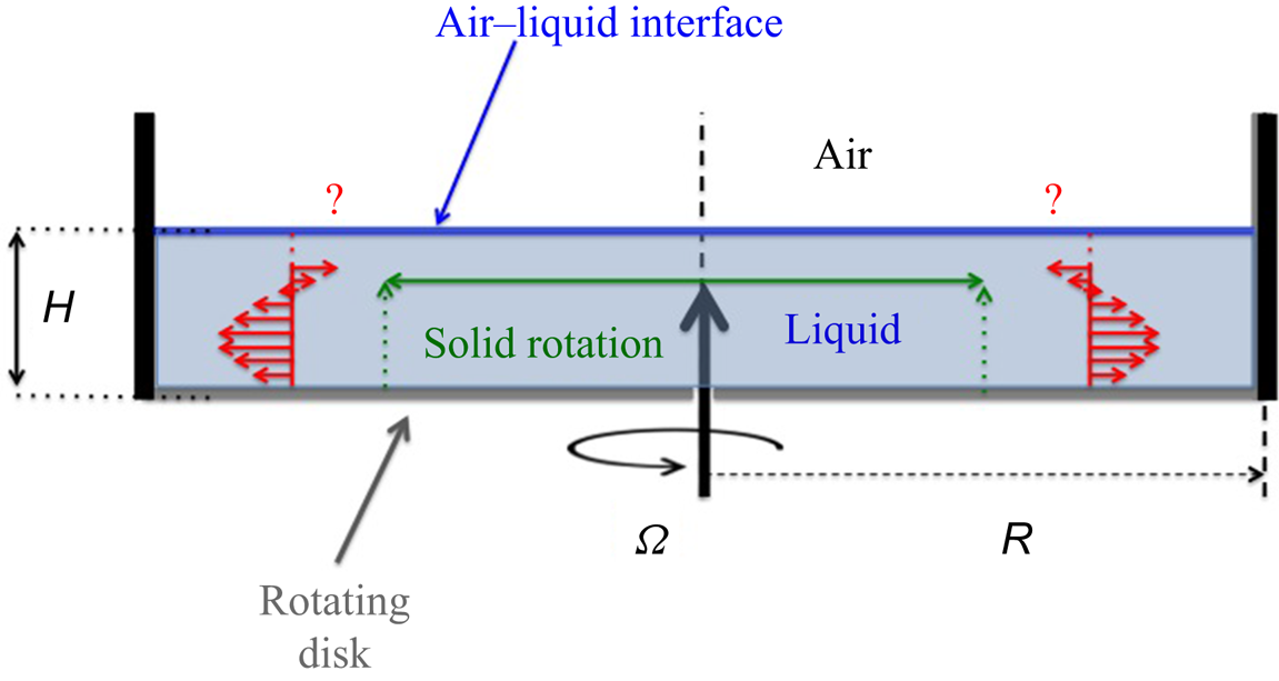
Figure 1. Sketch of the flow over a rotating disc with fixed cylindrical sidewall, with geometrical parameters indicated. The exact boundary condition at the air–liquid interface in the presence of a polluted interface is being questioned.
Pointwise velocity measurements were made using a one-component laser Doppler velocimetry (LDV) device composed of a Dantec laser linked to a BSAFlow processor. The liquid was seeded with Dantec 10  ${\rm \mu}{\rm m}$ diameter silver-coated hollow glass spheres. Optical deviation problems were fixed a posteriori using the method described by Huisman, van Gils & Sun (Reference Huisman, van Gils and Sun2012). The standard deviation ( $u_z^{rms}$) of the instantaneous axial velocity component was monitored at the location $(r=0.74\pm 0.01,z=0.5G)$, at an azimuthal position fixed in the laboratory frame. The choice of the axial component was dictated by the ease of optical access. As for visualisations, non-axisymmetric flow patterns were highlighted by injecting ink into the fluid. When a glycerol mixture was used as a working fluid, ink of lighter density did not sink and stayed at the interface. The syringe used to inject ink was carefully hung with the needle barely touching the fluid interface to avoid disturbing the flow. A 26G (0.26–0.464 mm) inside–outside diameter needle proved to be a good compromise for being small enough while injecting sufficient ink flow to be visible.
Lagrangian tracking of a small particle at the interface was also performed with the 60 % glycerol mixture. The tracer in question was either ink (as mentioned above) or a solid tracer consisting of a small portion (less than 1 mm in diameter) from the outer protective sheath of an electric cable. In the latter case, the sheath could accommodate an air bubble, which together with capillary effects ensured that it stayed at the liquid interface. The respective trajectories of the ink and the tracer were monitored by filming at 30 f.p.s. using an IDS UI 3370 CP camera ( $2048 \times 2048$ pixels) mounted above the liquid. Even though each of them was intrusive, the use of two different measurement techniques allowed us to cross-check and validate both trajectory and velocity. In particular, the good match indicated that, despite the non-negligible size of the particle, its superficial trajectory could be considered in a first approximation as non-inertial.
Whatever the liquid mixture used, no instability was detected below  $Re=1500$. Above this value, the experimental protocol was to increase $Re$ in steps by adjusting the rotation speed. Several step values were investigated: $1/3, 1/2, 1$ or $2$ r.p.m.. Each step was then observed and analysed over a time ranging from 20 to 90 min, which corresponded to at least 35 disc revolutions for water and 62 disc revolutions for the $60\,\%$ glycerol mixture. To improve the experimental reproducibility, the mixed up solution was stored for 1 to 3 days inside the vessel, with a cover plate on top to reduce contact between the air and the interface.
2.2. Numerical tools
In all numerical approaches deployed here, only the liquid phase was simulated in the non-deformable cylindrical domain  $\{(r,\theta,z) \in (0:1) \times (0:2{\rm \pi} ) \times (0:G)\}$. The height-to-radius ratio $G$ was fixed to 1/4. After non-dimensionalisation by the angular velocity $\varOmega$, the radius $R$, the liquid density $\rho$ and the dynamic viscosity $\mu$, the incompressible Navier–Stokes equations in the bulk of the flow can be written as
 \begin{gather} \boldsymbol{\nabla} \boldsymbol{\cdot} \boldsymbol u = 0, \end{gather}
 \begin{gather}\frac{\partial \boldsymbol u }{\partial t} + (\boldsymbol u \boldsymbol{\cdot} \boldsymbol{\nabla})\boldsymbol u ={-} \boldsymbol{\nabla}p + \frac{1}{Re} \nabla^2{\boldsymbol u}, \end{gather}
where  $Re=\rho \varOmega R^2/\mu$. The boundary conditions which are not discussed in this work concern the sidewall ( $r=1$) and the rotating bottom ( $z=0$), both characterised by no-slip. By contrast, we have not yet specified the boundary conditions used at the liquid–gas interface located at $z=G$. The several codes described below can deal with the classical types of boundary conditions such as Neumann, Dirichlet or Robin. A given rotational symmetry $\mathcal {R}_m$, characterised by a fundamental azimuthal wavenumber $m> 0$, can be imposed such that the velocity field verifies
 \begin{equation} (\mathcal{R}_m{\boldsymbol u})(r,\theta,z)={\boldsymbol u}\left(r,\theta+\frac{2{\rm \pi}}{m},z\right)={\boldsymbol u}(r,\theta,z).\end{equation}
 Steady states are defined by  $\partial _t {\boldsymbol u}={\boldsymbol 0}$ in (2.2). They were identified numerically using a Newton solver. The spatial discretisation in this solver is based on a Cartesian finite difference representation in primitive variables using the exact same boundary conditions as above. The code has been validated against the formulation used by Kahouadji (Reference Kahouadji2011). It yields a numerical estimation of the base flow whose associated velocity field can be written $(U_r,U_{\theta },U_z)$ and depends on $r$ and $z$ only. The stability analysis of the base flow was carried out using an Arnoldi algorithm described in Appendix B.
As for the unsteady nonlinear simulations, we used the direct numerical simulation (DNS) code Sunfluidh developed for incompressible flows, described in Appendix A. It is based on a projection method to ensure a divergence-free velocity field. The governing (2.1) and (2.2) were discretised on a staggered structured non-uniform grid using a finite volume scheme with a second-order centred formulation in space. A second-order Backward Euler Differentiation was used for time discretisation. The nonlinear simulations were conducted without any azimuthal symmetry imposed.
The grid consisted of  $160\times 180\times 160$ cells in $r, \theta$ and $z$, respectively. The timestep was set to ${\rm \Delta} t= 4 \times 10^{-3}$ in units of $\Omega ^{-1}$. In the radial direction, the grid cell size varied from $8\times 10^{-3}$ at $r=0$ to $1.2\times 10^{-3}$ at $r=1$, and from $6\times 10^{-4}$ at $z=0$ to $8\times 10^{-4}$ at $z=G$ with a maximum of $10^{-3}$ in the axial direction. The mesh was thus more refined near the periphery $r=1$, close to the rotating disc as well as near the interface. The discretisation was uniform in the azimuthal direction.
3. Are free-slip boundary conditions appropriate?
3.1. Statement of the problem
As mentioned in § 1, determining an exact or at least effective boundary condition at the liquid–gas interface is the main goal of this study. Although a derivation from first principles is possible, it would invariably clash with the indetermination of the actual experimental conditions. We adopt here first a purely phenomenological approach that focuses on consequences rather than causes: instead of deriving the boundary conditions analytically by assessing the underlying physical mechanisms at play, we choose to simply gather experimental evidence as to how these interfacial conditions can be approximated in practice. Importantly, we begin by considering the steady regime. This regime is encountered experimentally for  $Re=3300$, the value at which these Lagrangian experiments are reported.
3.2. A Lagrangian tracking experiment
The main idea behind the present Lagrangian tracking is to quantify one of the macroscopic consequences of the interfacial boundary conditions, namely the radial drift of non-inertial tracers. Two different experimental tracking techniques have been used, one using ink and the other with a solid tracer (the sheath from an electric cable described earlier). The respective trajectories of the ink and the tracer are displayed in a sequences of superimposed images in figure 2. The trajectories of the ink and the sheath are quantitatively similar after almost two revolutions of the bottom disc. This good match ensures that both tracers, despite their differences in relative weight and the fact that one diffuses while the other does not, behave almost as neutral fluid tracers and remain at the interface. These experimental trajectories are compared with the numerical trajectories predicted for a given set of boundary conditions. Because the dynamics is steady, these numerical trajectories are evaluated by first determining the base flow  ${\boldsymbol U}=(U_r,U_{\theta },U_z)$ corresponding to the boundary conditions imposed, using the Newton solver mentioned earlier. The trajectories are later integrated numerically from solving the two-dimensional autonomous equation $(\dot {r}_p,\dot {\theta }_p) =(U_r,U_{\theta }/r_p)$, where $(r_p,\theta _p)$ denotes the position of the particle in the interface plane $z=G$. In particular, the numerical trajectory corresponding to the free-slip conditions $\partial _z U_r=0$ and $\partial _z U_\theta =0$ is shown in red in figure 2. This trajectory circles inward until it saturates at a fixed radial location, at approximately $r=R/2$. By contrast, the ink and the sheath trajectories (departing from the same initial radius located near the periphery of the flow) also spiral in but they experience a much shorter radial drift, approximately one tenth of a radius in one revolution. The fourth trajectory displayed in figure 2 in green (labelled ‘ $U_r=0$’) corresponds to the trivial integration, over the same duration, of a tracer without any radial drift, i.e. with $U_r=0$ and $\partial _z U_\theta =0$ for all $r$. This last case corresponds also to the model of Spohn & Daube (Reference Spohn and Daube1991). One of the visual conclusions from figure 2 is that the small radial drift of the two experimental trajectories (ink and sheath) is much closer quantitatively to the vanishing radial drift of the new model than to the large radial drift of the stress-free model.

Figure 2. Lagrangian tracking experiment. Comparison between model and free-slip boundary condition, ink injection and particle tracking for  $Re=3300$, and trajectories predicted by the numerical integration of the tracer position for the stress-free model ( $\partial _z U_r=0$, red) and the new model ( $U_r=0$, green). The liquid in the experiment is a 60 % glycerol mixture. Photograph taken after the disc has achieved $1.94$ revolutions after ink injection.
The radial drift of the tracer makes it move along the planar interface. The tracer hence visits the whole range of radius values from the periphery to the central zone. Both radial and azimuthal position are monitored at every time. Given that the base flow is axisymmetric and steady, the respective radial and azimuthal Eulerian velocity profiles can easily be reconstructed using finite differences. They are respectively shown in figures 3(a) and 3(b). The velocity profiles predicted for the base flow by either free-slip (red solid line) or the present model (green solid line) have been added to the figure for comparison. Compared with figure 2, figure 3(a) has the advantage of displaying the entire  $r$-profile. As indicated by the two velocity components, the flow is in solid body rotation for $r<0.4$ in the models, whatever the boundary condition at the interface.

Figure 3. Same conditions and parameters as in figure 2. Velocity profiles  $U_r(r)$ (a) and $U_\theta (r)$ (b) at the interface $z=G$. The cyan solid line for the radial velocity profile is a fit of the experimental data using cubic spline functions.
The comparison of azimuthal velocity profiles  $U_{\theta }(r)$ in figure 3(b) shows a flawless match between the experimental profile and the prediction by the new model. The free-slip profile displays, in turn, a neat excess of azimuthal velocity in the interval $0.4< r<0.6$ not compatible with the measurements. As for the radial component, for the free-slip boundary condition, it departs from zero and reaches negative values down to $-$0.17 over the range $0.6< r<0.8$. This is to be compared with the radial tracer velocity measured experimentally, which departs from zero only for $r>0.6$ and does not exceed 0.03 in magnitude. The experimental radial velocity profile is hence reasonably well approximated by $U_r=0$ for all $0< r<1$, rather than by the free-slip profile. This highlights again the limited relevance of the free-slip boundary condition in the steady regime.
The tracer has a finite size and cannot legitimately be considered non-inertial, which suggests that the tracer drift velocity is not exactly the radial velocity of the fluid. As a verification, the tracer is also tracked in a range of radii  $[0.14 - 0.2]$, where the velocity field obeys solid body rotation (see figure 3b). The order of magnitude of the radial drift velocity of the tracer in this region is a measure of the inertial effects (here only owing to centrifugal acceleration). The mean value of the tracer drift velocity is $8.3 \times 10^{-4}$, which is barely visible on the scale of figure 3(a). It indicates that inertial effects have a weak influence on the radial fluid velocity measurements.
The Dirichlet condition  $U_r=0$ is only an approximation, and it is a relatively strong hypothesis. To better judge the quality of this approximation, an alternative radial velocity profile is suggested as a boundary condition. This new data-driven profile is obtained in figure 3(a) by simply fitting (rather than approximating) the experimental radial profile of $U_r$ for $Re=3300$ using cubic spline functions. The new profile $U_r^{exp}(r)$, compared with its experimental counterpart, displays the same variations yet in a smoother way. It can later be imposed directly in the numerical codes as another Dirichlet boundary condition $u_r(z=G)=U_r^{exp}(r)$. As a rough model allowed only in the frame of a robustness test, the same radial velocity profile is imposed independently of the value of $Re$.
$Re$.
3.3. Model boundary conditions for the steady base flow
The reasons why the usual free-slip boundary condition does not apply to the current set-up have been discussed by Lopez & Chen (Reference Lopez and Chen1998), Faugaret et al. (Reference Faugaret, Duguet, Fraigneau and Martin Witkowski2020) and Faugaret (Reference Faugaret2020). It is important to recall that the free-slip condition itself comes from an approximation of the force balance between the liquid and the gas at the interface. As the viscosity and surface tension of the gas phase are often neglected, the interfacial force balance reduces to the steady balance between viscous stresses and Marangoni forces in the liquid at every point of the interface.
Starting from the Boussinesq–Scriven surface fluid model for a Newtonian fluid–gas interface (Scriven Reference Scriven1960), assuming that the interface remains flat at all times, and under the hypothesis of negligible surface dilatational viscosity and surface shear viscosity (Hirsa, Lopez & Miraghaie Reference Hirsa, Lopez and Miraghaie2001), the force balance leads to the following boundary conditions:
 \begin{equation} \frac{\partial u_r}{\partial z} = \frac{1}{Ca}\frac{\partial \bar{\sigma}}{\partial r}, \quad \frac{\partial u_{\theta}}{\partial z} = \frac{1}{Ca}\frac{1}{r}\frac{\partial \bar{\sigma}}{\partial \theta},\quad u_z=0, \end{equation}
where  $\bar {\sigma }=\sigma /\sigma _0$, with $\sigma$ the surface tension of the liquid and $\sigma _0$ the reference surface tension. The capillary number is defined as $Ca =\mu \Omega R/\sigma _0$, with $\mu$ the dynamic viscosity. A closure $\sigma =f(c)$ for the surface tension $\sigma$ is necessary, here as a function of the concentration $c=c(r)$ only. The important physical property to capture in the closure is the decrease of $\sigma$ with increasing concentration, while the concentration $c(r)$ is governed by in-plane advection and diffusion only (Stone Reference Stone1990; Kwan et al. Reference Kwan, Park and Shen2010). It is also assumed that surfactants remain at the interface at all times and that they neither sink towards the bulk nor undergo desorption. This is justified for low enough pollutant concentrations in the steady regime (Bandi et al. Reference Bandi, Akella, Singh, Singh and Mandre2017). The effective radial velocity profile resulting from this interplay is not trivial. Faugaret et al. (Reference Faugaret, Duguet, Fraigneau and Martin Witkowski2020) have demonstrated for the base flow for another value of $G$, in the limit of large concentrations, the radial profile evolves non-uniformly towards $U_r=0$. We assume that the same result also holds here for $G=1/4$. As for the azimuthal velocity profile, (3.1b) together with axisymmetry yields $\partial _z U_{\theta }=0$, like in the free-slip boundary conditions. This is perfectly consistent with the findings of Miraghaie et al. (Reference Miraghaie, Lopez and Hirsa2003) in a related geometry. The impermeability condition yields $U_z=0$.
The suggested synthetic boundary conditions for the base flow hence write:
 \begin{equation} U_r=0, \quad \frac{\partial U_{\theta}}{\partial z} = 0, \quad U_z=0.\end{equation}
3.4. Comparison of stationary velocity profiles
The steady base flow with either the free-slip, the new model or the fitted boundary condition has been computed for  $Re=3300$ using the Newton solver. The corresponding $z$-profiles for the radial component are shown in figure 4 for increasing values of $r$, i.e. from the axis towards the sidewall. For all values of $r$, the three profiles match very well from $z=0$ up to a given value dependent on $r$. Above this value of $z$, the free-slip profile deviates significantly from the two other base flow profiles. This $r$-dependent match is consistent with the radial development of the Ekman-like boundary layer on the rotating plate. Remarkably, the volumetric profile resulting from the fitted condition $U_r=U_r^{exp}$ differs very little from the one induced by $U_r=0$, except very close to the interface.

Figure 4. Radial velocity profiles at  $r=0.55$ (a), 0.70 (b), 0.85 (c) for the base flow at $Re=3300$. Boundary conditions: free-slip (red); $U_r=0$ (green); radial profile fitted from experiments at the same value of $Re$ (cyan).
A qualitative comparison of the global distribution of  $U_r$ in the meridian plane is possible at that stage. The recirculation in the meridian $(r,z)$ plane is known to be caused by the axial gradients of $u_{\theta }$. These gradients primarily arise from the lack of azimuthal entrainment at the interface, so that the flow entrained by the rotating disc is slowed down by the friction at the sidewall. The recirculating meridian flow invariably takes, near the rotating bottom wall at $z=0$, the form of a radial flow outwards. Continuity imposes the flow to loop and recirculate inwards near the upper interface at $z=G$, with the exact profile in the upper half depending on whether free-slip or no-slip is imposed.
3.5. Unsteady regime
It is known from former investigations that for  $Re$ large enough, the axisymmetric base flow loses its stability. The resulting instability patterns are characterised by an integer $m$, the leading azimuthal wavenumber selected by the instability. Structurally, the corresponding modes display at saturation exactly $m$ off-centred co-rotating vortices. These vortices are clearly visible from above using ink in the experimental figures 5(a), 5(c), 5(d) and 5(f). The approximately circular ink trajectories in the off-centred vortices are a priori incompatible with the condition $U_r=0$, because vortices need a genuinely two-dimensional velocity field (note however that axial vorticity at the interface is not excluded because $\omega _z$ also contains, by definition, radial derivatives of $u_{\theta }$). As a consequence, the frozen model suggested by Spohn & Daube (Reference Spohn and Daube1991) becomes ill-adapted to unsteady simulations for which it requires a non-trivial generalisation.

Figure 5. Instability observed for  $Re=2100 (\textit {a},\textit {d},\textit {g}), Re=3300$ (b,e,h) and $Re=5545$ (c,f,i). (a,b,c) 60 % glycerol experiment, short time after ink injection. (d,e,f) Same experiment, long time after ink injection. (g,h,i) Top view of three-dimensional axial vorticity isolevels. The four blue and the four red isosurfaces are linearly spaced in $[- 0.016,-0.04]$ and [0.1,0.4], respectively.
New boundary conditions were suggested in the last part of the paper by Faugaret et al. (Reference Faugaret, Duguet, Fraigneau and Martin Witkowski2020) and used only in the context of linear stability analysis. This model assumes a decomposition of the velocity field  ${\boldsymbol u}=\boldsymbol {U} + \boldsymbol {u'}$ into an axisymmetric part ${\boldsymbol U}$ with $\partial _{\theta }\boldsymbol {U}=0$ and a residual perturbation $\boldsymbol {u'}$. Faugaret et al. (Reference Faugaret, Duguet, Fraigneau and Martin Witkowski2020) explicitly chose ${\boldsymbol{U}_{b}}$ as the base flow solution of the steady (2.1) and (2.2) (with $\partial _t=0$) and computed with the boundary condition $U_r=0$ at $z=G$. Such a solution is found either using the Newton method or by timestepping the unsteady equations under an axisymmetry assumption, because no axisymmetric instability occurs for the range of $Re$ investigated. The perturbation remains subject to the classical stress-free boundary condition $\partial _z u'_r=0$. This is different from the approach adopted by Miraghaie et al. (Reference Miraghaie, Lopez and Hirsa2003), where the doubt about the stress-free boundary conditions is on the perturbations rather than on the base flow like in the present model.
In the present study, we also perform unsteady nonlinear simulations based on a pre-existing well-tested numerical code. For this purpose, another decomposition  $\boldsymbol {u}=\bar {\boldsymbol {U}}+\tilde {\boldsymbol {u}}$ into mean flow $\bar {\boldsymbol {U}}$ and fluctuation $\tilde {\boldsymbol {u}}$ is preferred for its computational simplicity. The mean flow $\boldsymbol {U}(r,z,t)$ is defined as the instantaneous azimuthal average
 \begin{equation} \bar{\boldsymbol{U}}(r,z,t)=\frac{1}{2{\rm \pi}}\int_{0}^{2{\rm \pi}} {\boldsymbol u}(r,\theta,z,t) \, \textrm{d} \theta. \end{equation}
In practice, this average needs only be performed at the interface  $z=G$. Mean flow and base flow do not strictly coincide except in the linearised regime around the steady axisymmetric solution $\boldsymbol {U_b}$, where the velocity field can be written ${\boldsymbol u}(r,\theta,z,t)={\boldsymbol U_b}(r,z) + \varepsilon \tilde {\boldsymbol {u}}(r,z,\theta,t) + O(\varepsilon ^2)$. At order $O(\varepsilon )$, because nonlinear interactions of the perturbations to the base flow are neglected, $\bar {\boldsymbol {U}} \approx \boldsymbol {U_b}$ because $<\tilde {\boldsymbol {u}}>=0$.
The suggested synthetic boundary conditions for the mean flow in the linear regime can be written, as for the base flow, by
 \begin{equation} \bar{U}_r=0, \quad \frac{\partial \bar{U}_{\theta}}{\partial z} = 0, \quad \bar{U}_z=0.\end{equation}
 The fluctuating velocity field  $\tilde {\boldsymbol {u}}(r,\theta,t)$ is however subject to the regular stress-free boundary conditions
 \begin{equation} \frac{\partial \tilde{u}_r}{\partial z} =0, \quad \frac{\partial \tilde{u}_{\theta}}{\partial z} = 0, \quad \tilde{u}_z=0.\end{equation}
This full model amounts to neglecting the effect of the surfactants on the fluctuations while it is fully taken into account for the mean part.
4. Bifurcations
In this section, we present a joint experimental/numerical investigation of the onset of unsteadiness. The numerical approach is based on the model suggested in § 3.5 and detailed in Appendices A and B.
4.1. Modal selection in experiments
We begin by explaining the modal selection as observed in the experimental campaign. The protocol was carefully designed with measurements as  $Re$ is increased in small steps. We report here first only stable states that can be observed on long enough timescales from 1 to 3–4 days after the preparation of the solution. As $Re$ is increased from rest, the first instability is well identified. It corresponds to the instability of a mode with $m=3$. Its onset in Reynolds number $Re_c^{(m=3)}$ depends on the experimental details such as the amount of glycerol in the solution: for a glycerol amount of 60 $\,\%, Re_c^{(m=3)} \approx 1550\pm 50$, while for no glycerol it lies in the range $1600 - 1700$. This is to be compared with the value of $Re \approx 2000$ at which the instability was reported experimentally by Lopez et al. (Reference Lopez, Marques, Hirsa and Miraghaie2004) and Vogel et al. (Reference Vogel, Miraghaie, Lopez and Hirsa2004). The same instability was also identified numerically by Kwan et al. (Reference Kwan, Park and Shen2010) using a quadratic surfactant model, although some parameters (which need to be calibrated) have no equivalent in our study.
The exact threshold value turns out to be very sensitive to the experimental conditions. The mode  $m=3$ is observed visually and attested in the LDV time series up to a second critical value of $Re \approx 2500$ for glycerol and 3100 for water. Above this threshold, the axisymmetric base flow is recovered over a finite range of values of $Re$ called a stability island. Above a second onset value $Re_c^{(m=2)}$, the base flow is again unstable, yet to a mode with symmetry $m=2$. This onset value varies within the $Re$-interval 3800–4800, and depends on the direction in which $Re$ is varied. This is a clear signature of hysteresis that will be tackled later. Measurements were not attempted beyond $Re=5600$ because for the glycerol mixture, the Froude number ( $\varOmega ^2 R/g$, where $g$ is gravity) is no longer small and the validity of a flat free-surface approximation becomes questionable. A sequence of flow visualisations covering the three main zones ( $m=3$, stability island, $m=2$) is shown in figure 5 for $Re=2100$, 3300 and 5545. In the first row, the photographs are taken a few revolutions after ink injection, but the number of peripheric vortices is already well identified. In the second row, the photographs are taken at a later time at which the ink patterns are only diffusing. At this later time, the ink ends up concentrated in the core of these vortices which, as a consequence, appear thinner in figure 5(d) and 5(f). This introduces a qualitative distinction between short and long observation times, related to the typical shearing timescale of the ink. Visualisations stemming from the nonlinear simulations of the new model have been included in the last row for the exact same values of $Re$. These visualisations will be discussed later.
We briefly comment on the robustness of these results with respect to experimental conditions, especially the age of the aqueous preparation. Two extreme situations can occur if the preparation is either too young or too old. If the measurements are performed on the same day as the preparation, the variability of the results is much higher and the modal selection is impacted in a way inconsistent with the tracing of a reproducible bifurcation diagram. Instead of the first unstable mode  $m=3$, LDV measurements as well as visualisations indicate the occurrence of modes $m=2$ in water, or even $m=4$ in glycerol mixtures (the latter with amplitudes barely higher than the noise level). The higher variability and the possible occurrence of an $m=4$ mode were confirmed experimentally for lower glycerol contents of $20\,\%$ and $40\,\%$. The dependence of the modal selection on the quality of water has been raised by Lopez et al. (Reference Lopez, Marques, Hirsa and Miraghaie2004). Indeed, if the preparation is left at rest in the laboratory for longer than a day, the modal selection favours the appearance of an $m=3$ mode at onset, whatever the fluid. The protocol of waiting for 1 day to obtain a contaminated surface is consistent with that of Bernal et al. (Reference Bernal, Hirsa, Kwon and Willmarth1989). Fluid ageing also impacts the selection of the second unstable mode, especially the hysteresis: beyond 3–4 days, in glycerol experiments with descending $Re$ (see Appendix C), a mode $m=2$ has been identified to persist down to values of $Re$ for which a stable base flow is expected. This mode $m=2$ may even overlap completely with the stability island. This confirms that the instantaneous chemistry of the interface does influence crucial stability characteristics such as the modal selection. The difficulties associated with the accurate tracking in time of the chemical composition reinforce the need for a simple model. In the remainder of this article, to avoid the complications associated with multistability, we only focus on the time window between 1 and 3 days where the experimental variability is minimal and the results are self-consistent.
4.2. Linear stability analysis
The linear stability analysis (LSA) of the base flow is the classical numerical way to predict the modal selection from the governing equations, at least in the presence of supercritical bifurcations. Assuming a perturbation to the base flow in the form  $\textrm {e}^{\lambda t + \textrm {i}m\theta }$, a mode is unstable if the real part $\textrm {Re}(\lambda )$ of the complex associated eigenvalue $\lambda$ is strictly positive, else it is linearly stable. LSA parametrised by $Re$ was performed for the two main models, respectively free-slip and the model with $U_r=0$. $\textrm {Re}(\lambda )$ is shown versus $Re$ in figures 6(a) and 6(b). Only the modes with $m=2$, 3 and 4 were considered. For the free-slip model, the first unstable mode is the mode $m=2$ above $Re=3505$. No branch of $m=3$ is unstable before $Re=4755$. In contrast, for the new model, a branch of $m=3$ modes destabilises somewhere between $Re=1580$ and $2650$. The next instability involves a mode $m=2$ from $Re=3635$ on. All critical Reynolds numbers are given rounded by $\pm 5$, with an accuracy of a few percent (see Appendix B). They have been computed using a grid of $160\times160$ cells in $r$ and $z$ like in the nonlinear simulations. The curve $\textrm {Re}(\lambda )=f(Re)$ for the $m=2$ mode appears in figures 6(a) and 6(b), common to the two models. However, the most unstable $m=3$ branch seems specific to the new model and has no obvious stress-free counterpart. Additionally, the experimental selection mimics qualitatively the stability of the base flow for the new model, whereas the instabilities of the stress-free model are not consistent with the experimental observations. In particular, the stress-free model does not predict the first $m=3$ instability and, as a consequence, misses the instability island altogether.

Figure 6. Growth rate  $\textrm {Re}(\lambda )$ of the least damped eigenmodes versus $Re$ (blue, $m=2$; red, $m=3$; green, $m=4$). (a) Stress-free boundary condition; (b) new boundary condition (open symbols) and fitted boundary condition (closed symbols). The thick red dots correspond to the values of $Re$ with visualisations in figure 5.
Eventually, the robustness of the bifurcation diagram in figure 6(b) was investigated by considering, instead of the base flow predicted by the exact model with  $U_r=0$, the base flow reconstructed from the fitted experimental profile at the interface (see § 3.3). Although the reconstructed velocity fields differ (see figure 4), their stability characteristics for $m=2$ and 3 are very similar, as shown in figure 6(b). In particular, the modal selection $m=3$, 0 and 2 obtained as $Re$ increases is common to both new models whereas it is missed by the free-slip model.
4.3. Quantitative bifurcation diagrams
If the modal selection process can be well explained and predicted by linear theory, quantitative bifurcation diagrams demand nonlinear simulations. We demonstrate below that nonlinear simulations of the suggested model respect the modal selection predicted by LSA, but also match well the amplitude levels measured experimentally.
The main quantity measured experimentally using LDV is the pointwise axial velocity at a given location in the fixed laboratory frame. In such a frame, the saturation of a mode with both  $\textrm {Im}(\lambda )$ and $m$ non-zero leads in the simplest scenario to a rotating wave with angular phase velocity $\textrm {Im}( - \lambda )/m$. The amplitude of the associated time oscillations is characterised by the standard mean deviation of the measured velocity probe, denoted $u_z^{rms}$. This quantity is depicted in figure 7. Two different campaigns corresponding to two different fluids are reported: water as well as a water–glycerol mixture with 60 $\,\%$ glycerol in mass. The same quantity $u_z^{rms}$ was measured in the nonlinear simulations at essentially the same measurement station $(r,z)=(0.8,0.125G)$. For both fluids and for values of $Re$ around 3000, the experimental noise represents less than 0.5 $\,\%$ of the amplitude. Both experiments as well as the DNS display a clear bump in their bifurcation diagram corresponding to the occurrence of the saturated $m=3$ mode. All three datasets predict a maximum amplitude of approximately 0.0097–0.012 located in the $Re$-interval 2000–2400. The maximum amplitude obtained for water occurs at the larger Reynolds number. Considering the differences between the experimental fluids and the crudeness of the model, this appears hence as a quantitatively decent comparison, especially when compared with the stress-free model which does not capture the instability with $m=3$. The stability island is also well captured by the nonlinear simulations, although they tend to overpredict its width in the case of water.

Figure 7. Amplitude bifurcation diagram. Temporal standard deviation  $u_z^{rms}$ versus $Re$. Experimental LDV measurements at location $(r,z)=(0.74 \pm 0.01,0.5G)$ with water (blue dots) or 60 % glycerol–water mixture (red dots) versus DNS using the new model (black lines) at location $(r,z)=(0.8,0.5G)$. The blue and red solid lines correspond to local second-order polynomial fits. A hysteresis area has been indicated symbolically in grey.
The occurrence of the  $m=2$ instability is harder to quantify because of the presence of a hysteresis zone. The bounds of this hysteresis zone have been estimated experimentally by raising $Re$ up to 5600, and decreasing $Re$ from there in steps of 100 to 200. The DNS data confirms this hysteresis by revealing the existence of two different amplitude levels, the lower one with $u_z^{rms} \approx 5 \times 10^{-3}$ and the higher one with amplitudes closer to $3 \times 10 ^{-2}$. Such a distinction is not possible in the present experiment, because the level $5 \times 10^{-3}$ appears comparable to the noise level. The details of the experimental and numerical protocols are given in Appendix C.
The angular phase velocities for the rotating wave, estimated from experiments, DNS and LSA, compare very well. In the experiments at  $Re=2100$ and $Re=5545$, the modal structure (respectively $m=3$ and $m=2$) precesses in the prograde direction with a lag, as it propagates at angular velocity 0.65 (respectively 0.55). The corresponding values are 0.63 (respectively 0.54) in DNS and 0.64 (respectively 0.54) in LSA, which suggests that the angular phase velocity is weakly affected by nonlinearity. Further analysis of the spectrum at $Re=5545$ shows that in addition to the dominant modes $m=2$ and $m=3$, only few harmonics are of significant energy level. These values also compare well with the angular velocity of 0.62 reported by Miraghaie et al. (Reference Miraghaie, Lopez and Hirsa2003) for $Re=2000$. We are confident that the structures identified both experimentally and using the new model correspond to the same mode.
Furthermore, the location of the vortical structures can be compared between experiments and numerics by monitoring respectively the location where the ink (respectively a passive tracer) concentrates (figures 5d and 5f). In the rotating frame of the wave, the numerical velocity field at the interface is steady but not incompressible in the plane. The vortex centres in this plane stand here as stable fixed points for the Lagrangian motion of passive tracers. These points are located at a radius 0.62 for  $Re=2100$ and 0.65 for $Re=5545$, whereas experiments with ink suggest the respective values of 0.64 and 0.68. These values are consistent with the location of the extrema of axial vorticity below the interface (see figures 5g and 5i). Despite a small shift in the radial position, the match is fair given the experimental uncertainty.
We define next the instantaneous flow rate  $Q(t)$ through any meridian cross-section by
 \begin{equation} Q=\int_{0}^{G}\int_0^{1}u_{\theta}\, \textrm{d} r\, \textrm{d} z.\end{equation}
In practice, we use a normalised form of  $Q$, namely $Q^*=Q/Q_0$, where $Q_0=\iint r\, \textrm {d} r\, \textrm {d} z$ is the flow rate corresponding to the equivalent solid body rotation flow with the same angular velocity. Because the present flow is entrained only by the rotating disc, less fluid is entrained compared to solid-body rotation, and hence $0< Q^*<1$. Here, $Q^*$ can not be estimated experimentally, but its estimates from DNS are reported in figure 8 versus $Re$. One advantage of the quantity $Q^*$ over the variance of $u_z$ is that rotating waves are associated with fixed points of $Q^*$ rather than limit cycles, while unsteady time series of $Q^*(t)$ are the signature of temporally modulated rotating waves. Two supplementary modulational instabilities of the rotating wave with $m=2$ have been identified in figure 8, one with very small modulational amplitude and another one (which we refer to as ‘lower branch’) with larger amplitudes, bifurcating from a new (disconnected) branch of rotating waves. The existence of several such branches is consistent with the hysteresis mentioned in the description of figure 7. Figure 9 contains an additional characterisation of the states found along the lower branch of figure 8, extracted from the times series of $Q^*(t)$. It contains notably the modulation amplitude $A_{Q^*}$ versus $Re$, extracted from the min–max extrema and the main modulation frequency $f_0(Re)$ deduced from the frequency spectrum. The continuous growth of the amplitude versus $Re$ in panel (a) and the almost constant frequency in panel (b) both support the emergence of this branch via a supercritical Neimark–Säcker bifurcation. Characteristics of the modulational states found along the lower branch, such as their amplitude and temporal frequency, are reported in figure 9. The onset of the modulation for $m=2$ lies at $Re=Re_{M}^{(m=2)}$ between 4250 and 4400. The modulation amplitude increases apparently with $Re$ but was not monitored beyond $Re=5500$ (note that the snapshot displayed in figure 5(i) corresponds to a time prior to the development of the temporal modulation). The experimental measurements are not accurate enough to reveal whether this modulation is present or not, at least when $Re$ is sufficiently low. Interestingly, preliminary nonlinear simulations of the stress-free model with similar resolution have indicated a similar modulational instability (Faugaret Reference Faugaret2020). The modulation of the saturated mode $m=2$ seems thus to be common to both models, although a deeper investigation of the limitations of the model would be necessary to conclude.

Figure 8. Normalised azimuthal flow rate  $Q^*$ versus $Re$ (DNS). Stable steady axisymmetric base flow (solid green), unstable axisymmetric base flow (dashed green), rotating wave $m=3$ or lower/upper branch $m=2$ mode (blue dots) and time-modulated $m=2$ mode (red dots). The vertical bars indicate the temporal fluctuations.

Figure 9. Characteristics of modulated states along the lower branch of figure 8 as a function of  $Re$: (a) amplitude $A_{Q^*}(Re)$; (b) frequency $f_0(Re)$.
5. Conclusions
The present experimental and numerical study sheds light on the effect of arbitrary pollutants on the stability of a model swirling flow. This flow is generated by a rotating bottom lid and open at the top. It was originally selected because of previously ambiguous conclusions about the selection of the most unstable modes at least for small aspect ratios. The modal mismatch, as in Faugaret et al. (Reference Faugaret, Duguet, Fraigneau and Martin Witkowski2020), is attributed to the small but unavoidable presence of pollutants on the free surface. Although small and poorly measurable in practice, these pollutants turn out to have a strong influence on the stability of the flow. Simulating the whole system of equations together with the transport of the pollutants (modelled as simple-species surfactants) should include the precise knowledge of the chemical composition of the interface, a Marangoni closure and many physical constants to be determined. We circumvent this complexity by assuming a parameter-free description both easily accessible and easy to implement in a numerical code. We suggest hence a Dirichlet boundary condition for the radial velocity field alone. The steady base flow and the perturbation are treated separately: the radial velocity is assumed to vanish for the base flow while for the perturbation, the usual stress-free conditions are retained. This paper explores the nonlinear dynamics of the flow for an aspect ratio of  $G=1/4$, as in Hirsa et al. (Reference Hirsa, Lopez and Miraghaie2001), both using an experimental set-up and an adapted DNS code with the aforementioned boundary condition. The stability thresholds for modes with different rotational symmetries are well reproduced by the model, where the stress-free boundary conditions fails quantitatively as well as qualitatively. The experimental bifurcation diagram, including as $Re$ increases a saturated $m=3$ mode followed by a stability island and the emergence of an $m=2$ mode, are all well reproduced quantitatively by the nonlinear simulations. Both models predict a modulational instability of the $m=2$ wave, a result yet to be verified experimentally. The different modal selections and the associated nonlinear dynamics result from subtle changes in the structure of the base flow. The instability of the $m=3$ mode and the stability island are both absent in the more common stress-free model. This emphasizes the relevance of the new model. However, the applicability of this new model has also limitations revealed by the comparison with experiments. Aqueous solutions either too fresh (yet unaffected by the adsorption of pollution) or too old possess instability features not captured by the model. For a too young liquid mixture, the modal selection is no longer predicted by the model, with modes $m=2$ and $m=4$ replacing the mode $m=3$ for the same parameters. For a too old liquid mixture instead, the width of the hysteresis zone overlaps with the stability island and the bifurcation diagram of figure 7 becomes invalid. The experimental variability appears also less pronounced for tap water than for the water–glycerol mixtures. This suggests, for the present experimental water set-up, a need to select a specific temporal window from one to 3–4 days such that experimental variability is minimised. This result is experiment-dependent but has proven robust regardless of the exact water mixture considered. Future desirable developments of this modelling approach include non-flat interfaces when the Froude number increases (Kahouadji & Martin Witkowski Reference Kahouadji and Martin Witkowski2014; Carrión et al. Reference Carrión, Herrada, Shtern and López-Herrera2017; Tasaka & Iima Reference Tasaka and Iima2017) and possible dewetting regimes (Jansson et al. Reference Jansson, Haspang, Jensen, Hersen and Bohr2006; Mougel et al. Reference Mougel, Fabre, Lacaze and Bohr2017; Yang et al. Reference Yang, Delbende, Fraigneau and Martin Witkowski2019, Reference Yang, Delbende, Fraigneau and Martin Witkowski2020; Rashkovan et al. Reference Rashkovan, Amar, Bieder and Ziskind2021). Using a multiphase formalism, Yang et al. (Reference Yang, Delbende, Fraigneau and Martin Witkowski2020) have shown that the motion in the gas phase above the interface is not relevant. However, the influence of denser fluids, as in the recent numerical simulations of Carrión et al. (Reference Carrión, Naumov, Sharifullin, Herrada and Shtern2020), should be investigated. Two-dimensional particle image velocimetry, as used in the same flow set-up by Miraghaie et al. (Reference Miraghaie, Lopez and Hirsa2003) in horizontal planes or by Carrión et al. (Reference Carrión, Naumov, Sharifullin, Herrada and Shtern2020) in meridian planes, could be a complementary way of analysing experiments. The approach developed in the present paper should also be generalised to non-axisymmetric geometries.
Acknowledgements
The authors thank the technical team CTEMO at LISN for their help with the experimental facility.
Funding
This work was supported by the French Agence Nationale de la Recherche under the ANR ETAE Project No. ANR-16-CE08-0011. HPC resources from GENCI-IDRIS (Grant No. 2017-2a10308) are also acknowledged.
Declaration of interest
The authors report no conflict of interest.
Appendix A. Numerical methods for nonlinear simulations
We present in this appendix the main features of the numerical methods used in the code called Sunfluidh to solve the incompressible Navier–Stokes equations in 3-D cylindrical geometry. We first detail the time-marching procedure to estimate the velocity field at each time step (here, for simplicity  ${\rm \Delta} t$ is assumed constant). We then present the projection method used to ensure a divergence-free velocity field. We conclude with the discrete operators involved in the Navier–Stokes equations in a 3-D cylindrical geometry.
A.1. Time-marching procedure
The time-marching procedure is based on the second-order backward differentiation formula. The viscous terms are treated implicitly to increase the numerical stability with respect to the timestep. We obtain the time-discrete system:
 \begin{equation} \frac{3\boldsymbol{u^{n+1,*}}-4\boldsymbol{u^{n}}+\boldsymbol{u^{n-1}} }{2{\rm \Delta} t}+ \boldsymbol{F_u^{n,n-1}}={-}\boldsymbol{G_p^n} + \boldsymbol{ Lu^{n+1} }, \end{equation}
where the superscripts  $n+1, n$ and $n-1$ denote successive time steps, $\boldsymbol {G_p^n}$ is the discrete pressure gradient at $n{\rm \Delta} t, \boldsymbol {Lu^{n+1}}$ is the viscous term and $\boldsymbol {F_u^{(n,n-1)}}$ is the discrete convection flux estimated at time $(n+1){\rm \Delta} t$ from the linear extrapolation
 \begin{equation} \boldsymbol{F_u^{n,n-1}}= 2\boldsymbol{F_u^{n}} -\boldsymbol{F_u^{n-1}}. \end{equation}
The system is rearranged in an incremental form
 \begin{equation} \boldsymbol{H_u\delta u}= \left(\mathbb{1}- \frac{2{\rm \Delta} t}{3} \boldsymbol{\cdot} \boldsymbol{L}\right) \delta \boldsymbol{u}= \boldsymbol{S^{n,n-1}} \boldsymbol{\cdot} \frac{2{\rm \Delta} t}{3}, \end{equation} $\delta \boldsymbol {u}= \boldsymbol {u^{n+1,*}} - \boldsymbol {u^{n}}$ and $\boldsymbol {S^{n,n-1}}$ is the right-hand side term which gathers all explicit contributions from the time discretisation, the convection terms and the explicit contributions of the viscous terms. We specify each velocity component is solved separately what leads to the resolution of three independent systems $H_i\delta u_i = \frac {2}{3}{\rm \Delta} t \cdot S_i^{n,n-1}$ with $i= r, \theta, z$.
As the spatial discretisation is carried out using a second-order centred scheme (see § A.3.2),  $H_i$ can be approximated by means of a factorisation procedure that leads to the resolution of three tridiagonal systems (one per direction). This technique is based on the work of Peaceman & Rachford (Reference Peaceman and Rachford1955) that has been then adapted and largely used for different applications (see for instance Beam & Warming Reference Beam and Warming1976; Kim & Moin Reference Kim and Moin1985; Verzicco & Orlandi Reference Verzicco and Orlandi1996). At the end of this step, the velocity field $\boldsymbol {u^{n+1,*}}$ is not yet divergence-free.
A.2. Projection method
The divergence-free velocity field  $\boldsymbol {u^{n+1}}$ is obtained by means of a projection method (Guermond, Minev & Shen Reference Guermond, Minev and Shen2006) used in an incremental form proposed by Goda (Reference Goda1979). This consists in solving the Poisson equation
 \begin{equation} \nabla^{2} \phi = \frac{\boldsymbol{\nabla} \boldsymbol{\cdot} \boldsymbol{u^{n+1,*}} } {{\rm \Delta} t}, \end{equation}
with zero normal derivative as boundary condition. The pressure and the velocity fields are thus updated between time  $n$ and $n+1$ according to
 \begin{gather} p^{n+1}= p^n+\phi, \end{gather}
 \begin{gather}\boldsymbol{u^{n+1}}= \boldsymbol{u^{n}}- \frac{2 {\rm \Delta} t}{3} \boldsymbol{\nabla} \phi - \frac{1}{Re}\boldsymbol{\nabla} \boldsymbol{\cdot} \boldsymbol{u^{n+1,*}}. \end{gather}
The resolution of the Poisson equation is performed using a direct method based on a Fourier expansion along the azimuthal direction coupled with a partial diagonalisation technique. This method is based on the work of Haidvogel & Zang (Reference Haidvogel and Zang1979) and has been used for instance by Barbosa & Daube (Reference Barbosa and Daube2005).
A.3. Spatial discretisation
A.3.1. Grid and coordinates
The Navier–Stokes equations are discretised on a staggered grid in cylindrical geometry. The indexation is defined as  $r_i, \theta _j$ and $z_k$ for the radial, azimuthal and axial coordinates, respectively. For each cell $\mathcal {C}(i,j,k)$, the scalar quantities (i.e. the pressure $P$) are evaluated at the cell centre whereas the velocity components ( $u_r, u_\theta, u_z$) are evaluated at the centre of cell faces, see figure 10(a). For the cells adjacent to the axis, only the radial velocity component is evaluated at the axis (see figure 10b).

Figure 10. Coordinate location and positions of the physical quantities evaluated in the cells  $\mathcal {C}(i,j,k)$ (black tag, scalar quantities; red tags, velocity components). Cells away from the axis (a). Cells adjacent to the axis (b).
The relations between the radial coordinate sets are given by
 \begin{gather} r_{i} = \tfrac{1}{2}(r_{i+{1}/{2}}+r_{i-{1}/{2}}) , \end{gather}
 \begin{gather}{\rm \Delta} r_{i}= r_{i+{1}/{2}}-r_{i-{1}/{2}}, \end{gather}
 \begin{gather}{\rm \Delta} r_{i+{1}/{2}}=r_{i+1}-r_{i}. \end{gather}
For the sake of simplicity, we suppose a regular distribution along the radius. We thus have  ${\rm \Delta} r_{i,j,k}={\rm \Delta} r_{i+{1}/{2},j,k}= {\rm \Delta} r$. The same convention is considered to define the azimuthal ( $\theta$) and axial ( $z$) coordinates along the $j$ and $k$ directions, respectively.
A.3.2. Discrete operators
The operators applied to the pressure  $P$ and velocity components $(u_r,u_{\theta },u_z)$ are discretised using a second-order centred scheme. For the sake of clarity, only the varying index is written down. We also define the space averaging operator in the $l$-direction for any quantity $\phi$ as
 \begin{equation} \bar{\phi}^l= \tfrac{1}{2}(\phi_{l+1}+\phi_{l}). \end{equation}
• The pressure gradient operator $\boldsymbol {G_P}$:
• in the
$u_r$ equation along the radial direction, $G_{i+{1}/{2}}(p) = ({p_{i+1}-p_{i}})/{{\rm \Delta} r}$;• in the
$u_\theta$ equation along the azimuthal direction, $G_{j+{1}/{2}}(p) =\! ({p_{j+1}\!-\!p_{j}})/({r_{i}{\rm \Delta} \theta })$;• in the
$u_z$ equation along the axial direction, $G_{k+{1}/{2}}(p) = ({p_{k+1}-p_{k}})/{{\rm \Delta} z}$.
• The velocity divergence operator (in the source term of the Poisson equation):
(A11)\begin{align} \boldsymbol{\nabla}\boldsymbol{\cdot} \boldsymbol{u}&= \frac{1}{r_i {\rm \Delta} r} ( r_{i+{1}/{2}} u_{r,i+{1}/{2}}-r_{i-{1}/{2}} u_{r,i-{1}/{2}}) \nonumber\\ &\quad + \frac{1}{r_i {\rm \Delta} \theta} ( u_{\theta,j+{1}/{2}} - u_{\theta,j-{1}/{2}} ) \nonumber\\ &\quad + \frac{1}{{\rm \Delta} z}( u_{z,k+{1}/{2}} -u_{z,k-{1}/{2}}). \end{align}• The convective flux balance in a conservative form
$F_{\boldsymbol u}= \boldsymbol {\nabla } \boldsymbol {\cdot } ( {}^t \boldsymbol {u} \otimes \boldsymbol {u})$:
• for
$u_r$ at $(i+\frac {1}{2},j,k)$,
(A12)\begin{align} F(u_r)&= \frac{1}{r_{i+{1}/{2}} {\rm \Delta} r} ( r_{i+1}\overline{u_r}^i_{i+1}\overline{u_r}^i_{i+1} - r_{i}\overline{u_r}^i_{i}\overline{u_r}^i_{i} ) \nonumber\\ &\quad + \frac{1}{r_{i+{1}/{2}} {\rm \Delta} \theta} ( \overline{u_r}^j_{j+{1}/{2}}\overline{u_\theta}^i_{j+{1}/{2}} - \overline{u_r}^j_{j-{1}/{2}}\overline{u_\theta}^i_{j-{1}/{2}} ) \nonumber\\ &\quad + \frac{1}{{\rm \Delta} z} ( \overline{u_r}^k_{k+{1}/{2}}\overline{u_z}^i_{k+{1}/{2}}- \overline{u_r}^k_{k-{1}/{2}}\overline{u_z}^i_{k-{1}/{2}} ) \nonumber\\ &\quad - \frac{u_{r,i+{1}/{2},j,k}^2}{r_{i+{1}/{2}}}; \end{align}• for
$u_\theta$ at $(i,j+\frac {1}{2},k)$,
(A13)\begin{align} F(u_\theta)&= \frac{1}{r_{i} {\rm \Delta} r}( r_{i+{1}/{2}}\overline{u_\theta}^i_{i+{1}/{2}} \overline{u_r}^j_{i+{1}/{2}} - r_{i-{1}/{2}}\overline{u_\theta}^i_{i-{1}/{2}} \overline{u_r}^j_{i-{1}/{2}} ) \nonumber\\ & \quad + \frac{1}{r_{i} {\rm \Delta} \theta} ( \overline{u_\theta}^j_{j+1}\overline{u_\theta}^j_{j+1} - \overline{u_\theta}^j_{j}\overline{u_\theta}^j_{j} ) \nonumber\\ & \quad + \frac{1}{{\rm \Delta} z}( \overline{u_\theta}^k_{k+{1}/{2}} \overline{u_z}^j_{k+{1}/{2}}- \overline{u_\theta}^k_{k-{1}/{2}} \overline{u_z}^j_{k-{1}/{2}} ) \nonumber\\ & \quad + \frac{\frac{1}{2}(\overline{u_r}^j_{i+{1}/{2}}+ \overline{u_r}^j_{i-{1}/{2}} )u_{\theta,i,j+{1}/{2},k} } {r_{i}}; \end{align}• for
$u_z$ at $(i,j,k+\frac {1}{2})$,
(A14)\begin{align} F(u_z)&= \frac{1}{r_{i} {\rm \Delta} r}( r_{i+{1}/{2}}\overline{u_z}^i_{i+{1}/{2}} \overline{u_r}^k_{i+{1}/{2}} - r_{i-{1}/{2}}\overline{u_z}^i_{i-{1}/{2}} \overline{u_r}^k_{i-{1}/{2}} ) \nonumber\\ & \quad + \frac{1}{r_{i} {\rm \Delta} \theta}( \overline{u_z}^j_{j+{1}/{2}} \overline{u_\theta}^k_{j+{1}/{2}} - \overline{u_z}^j_{j-{1}/{2}}\overline{u_\theta}^k_{j-{1}/{2}} ) \nonumber\\ & \quad + \frac{1}{{\rm \Delta} z}( \overline{u_z}^k_{k+1}\overline{u_z}^k_{k+1}- \overline{u_z}^k_{k}\overline{u_z}^k_{k} ). \end{align}
• The viscous terms (Laplacian operator) :
• for
$u_{r}$ at $(i+\frac {1}{2},j,k)$,
(A15)\begin{align} L(u_r) &= \frac{1}{r_{i+{1}/{2}}{\rm \Delta} r} ( r_{i+1} \frac{u_{r,i+{3}/{2}} - u_{r,i+{1}/{2}} } {{\rm \Delta} r} - r_{i} \frac{ u_{r,i+{1}/{2}} - u_{r,i-\frac{1}{2}} } {{\rm \Delta} r} ) \nonumber\\ & \quad + \frac{1}{r_{i+{1}/{2}}^2 {\rm \Delta} \theta} \left( \frac{u_{r,j+1}-u_{r,j} }{{\rm \Delta} \theta} - \frac{u_{r,j}-u_{r,j-1} }{{\rm \Delta} \theta} \right)\nonumber\\ & \quad + \frac{1}{{\rm \Delta} z} \left( \frac{u_{r,k+1}-u_{r,k} }{{\rm \Delta} z} - \frac{u_{r,k}-u_{r,k-1} }{{\rm \Delta} z} \right) \nonumber\\ &\quad - \frac{2}{r_{i+{1}/{2}}^2}\left(\frac{\overline{u_\theta}^i_{j+{1}/{2}} - \overline{u_\theta}^i_{j-{1}/{2}}}{{\rm \Delta} \theta}\right) \nonumber\\ &\quad -\frac{u_{r,i+{1}/{2},j,k}}{r_{i+{1}/{2}}^2}; \end{align}• for
$u_{\theta }$ at $(i,j+\frac {1}{2},k)$,
(A16)\begin{align} L(u_\theta) &= \frac{1}{r_{i}{\rm \Delta} r} \left( r_{i+{1}/{2}} \frac{u_{\theta,i+1} - u_{\theta,i} } {{\rm \Delta} r} - r_{i-{1}/{2}} \frac{ u_{\theta,i} - u_{\theta,i-1} } {{\rm \Delta} r} \right)\nonumber\\ & \quad + \frac{1}{r_{i}^2 {\rm \Delta} \theta} \left( \frac{u_{\theta,j+{3}/{2}}- u_{\theta,j+{1}/{2}}}{{\rm \Delta} \theta} - \frac{u_{\theta,j+{1}/{2}} -u_{\theta,j-{1}/{2}} }{{\rm \Delta} \theta} \right)\nonumber\\ & \quad + \frac{1}{{\rm \Delta} z} \left( \frac{u_{\theta,k+1}-u_{\theta,k} }{{\rm \Delta} z} - \frac{u_{\theta,k}-u_{\theta,k-1} }{{\rm \Delta} z} \right) \nonumber\\ & \quad + \frac{2}{r_{i}^2}\left(\frac{\overline{u_r}^i_{j+1} - \overline{u_r}^i_{j}}{{\rm \Delta} \theta} \right)\nonumber\\ &\quad -\frac{u_{\theta,i,j+\frac{1}{2},k}}{r_{i}^2}; \end{align}• for
$u_{z}$ at $(i,j,k+\frac {1}{2})$,
(A17)\begin{align} L(u_z) &= \frac{1}{r_{i}} \left(\frac{1}{{\rm \Delta} r} \left( r_{i+{1}/{2}} \frac{u_{z,i+1} - u_{z,i}}{{\rm \Delta} r} - r_{i-{1}/{2}} \frac{ u_{z,i} - u_{z,i-1} }{{\rm \Delta} r} \right) \right)\nonumber\\ & \quad + \frac{1}{r_{i}^2 {\rm \Delta} \theta} \left( \frac{u_{z,j+1}-u_{r,j} }{{\rm \Delta} \theta} - \frac{u_{z,j}-u_{z,j-1}}{{\rm \Delta} \theta} \right)\nonumber\\ & \quad + \frac{1}{{\rm \Delta} z} \left( \frac{u_{z,k+{3}/{2}}-u_{z,k+{1}/{2}} }{{\rm \Delta} z} - \frac{u_{z,k+{1}/{2}}-u_{z,k-{1}/{2}} }{{\rm \Delta} z} \right). \end{align}


A.4. Estimation of the radial velocity at the axis
Consistently with the numerical scheme detailed above, we need to estimate the radial velocity component  $u_r$ at the axis (see figure 10b). We rely on results from Lewis & Bellan (Reference Lewis and Bellan1990), where non-zero values of $u_r$ and $u_\theta$ at the axis are only related to the first (complex) azimuthal Fourier mode ( $\widehat {u_r}^{(1)},\widehat {u_\theta }^{(1)}$), for any $z$ plane. They showed that
 \begin{equation} \widehat{u_r}^{(1)}={-}i \boldsymbol{\cdot} \widehat{u_\theta}^{(1)} \quad (\textrm{with } i^2={-}1), \end{equation}
with
 \begin{equation} \widehat{u_\theta}^{(1)}=\lim_{r \to 0} \frac{1}{2{\rm \pi}}\int_0^{2{\rm \pi}} u_\theta(r,\theta) \, \textrm{e}^{{-\textrm{i}\cdot\theta}} \, \textrm{d} \theta. \end{equation}
Thanks to (A18) and (A19), we can estimate the values of  $u_r$ at the axis as a function of $\theta$, for any $z$ plane,
 \begin{equation} u_r(0,\theta)=\widehat{u_r}^{(1)}\textrm{e}^{{-}i\cdot \theta}= u_x^0\cos{\theta}+u_y^0\sin{\theta}, \end{equation}
linked to the Cartesian velocity components  $u_x^0$ and $u_y^0$. The latter are easily evaluated as
 \begin{gather} u_x^0=\lim_{r \to 0} -\frac{1}{2{\rm \pi}}\int_0^{2{\rm \pi}} u_\theta(r,\theta) \sin{\theta} \, \textrm{d} \theta \approx{-}\frac{1}{2{\rm \pi}} \sum_{j} \widetilde{u_\theta}_{j+{1}/{2}} \cdot\sin{\theta_{j+{1}/{2}}}\cdot {\rm \Delta} \theta, \end{gather}
 \begin{gather}u_y^0=\lim_{r \to 0} \frac{1}{2{\rm \pi}}\int_0^{2{\rm \pi}} u_\theta(r,\theta) \cos{\theta} \, \textrm{d} \theta \approx \frac{1}{2{\rm \pi}} \sum_{j} \widetilde{u_\theta}_{j+{1}/{2}} \cdot\cos{\theta_{j+{1}/{2}}}\cdot {\rm \Delta} \theta, \end{gather}
where  $\widetilde {u_\theta }_{j+{1}/{2}}$ is an extrapolation of $u_\theta$ to the axis along the radial direction.
Appendix B. Numerical methods for the linear stability analysis (LSA)
The numerical linear stability analysis is a two-step process. The first step consists in computing the nonlinear steady axisymmetric base flow for a given Reynolds number. The second step consists in finding the eigenmodes (eigenvalues and eigenvectors) associated with the Navier–Stokes equations linearised around the base flow for a given azimuthal mode  $m$. In our approach, we solve all the equations coupled as a large-size sparse linear system arising from the spatial discretisation. The choice of an efficient linear solver for non-Hermitian matrices is crucial for good performances.
B.1. Base flow computations
In the radial and axial directions, we have used the same spatial discretisation as for the nonlinear code Sunfluidh (cf. Appendix A). There is no temporal discretisation as only steady-state solutions are sought. Instead of solving a Poisson equation for the pressure, the divergence-free velocity field is obtained by solving the genuine velocity divergence operator on pressure grid nodes. This equation is coupled with the momentum equations. To avoid indeterminacy, a reference value for the pressure is imposed at an arbitrary grid point. The large algebraic nonlinear system of equations is solved using a Newton–Raphson algorithm. In the present configuration, five iterations are typically enough to obtain convergence to machine precision when starting from a well-chosen initial guess. This guess is either a zero velocity field if  $Re$ is small enough (typically $Re=500$) or a solution already computed for a near Reynolds number value. For each Newton–Raphson iteration, the algebraic system is solved owing to a direct sparse solver provided by common scientific packages, like Pardiso (Bollhöfer et al. Reference Bollhöfer, Schenk, Janalik, Hamm and Gullapalli2020) or Umfpack (Davis Reference Davis2004).
To validate the axisymmetric base flow, we also ran the three-dimensional Sunfluidh code at values of  $Re$ for which the flow is stable. At steady state and using the same grid in the meridional plane, both velocity fields match within $10^{-7}$. An alternate formulation, namely a vorticity-stream function, (in fact a third code detailed by Kahouadji, Houchens & Martin Witkowski Reference Kahouadji, Houchens and Martin Witkowski2011) has been used for cross-checking purposes. In this latter comparison, the same results are obtained below 1 %, which is consistent with the second-order finite difference discretisation used for both approaches.
B.2. Linear stability analysis
Once the base flow is obtained, the linearised Navier–Stokes equations together with the boundary conditions yield a generalised eigenvalue problem. To compute simultaneously a few selected eigenvalues, we use the implicit restarted Arnoldi method implemented in the Arpack library (Lehoucq, Sorensen & Yang Reference Lehoucq, Sorensen and Yang1998). We focus on the eigenvalues that have the largest real part by selecting the shift-and-invert strategy in Arpack. In addition to the tolerance on the computed eigenvalues, set to machine accuracy, other choices must be prescribed: the shift value, the number of eigenvalues sought around the shift and the maximal dimension of the Krylov subspace. The shift value is chosen along the imaginary axis and should ideally be close to the imaginary part of the most unstable eigenmode. Experimental observations are a useful guide, we chose  $-0.6$ m where $m$ is the azimuthal mode. Forty eigenvalues are computed for a Krylov subspace dimension of 100. The most unstable eigenvalue can be overlooked if inappropriate choices are made for the shift and the number of eigenvalues. However, in addition to experimental evidence, a posteriori checks with the nonlinear code Sunfluidh show consistency between all approaches, as detailed below.
B.3. Validations
The adequacy of the  $160 \times 160$ grid in $(r,z)$ was checked in a spatial resolution convergence study for the three Reynolds numbers where there is a transition from (or to) an axisymmetric base flow in figure 6(b). The critical values $Re_c$ of the Reynolds number are given in table 1 for the new model (open symbols).
Table 1. Critical Reynolds number values  $Re_c$: $Re_c^{(m=3)}$ for the transition from mode 0 to 3, $Re_c^{(m=0)}$ from 3 to 0 and $Re_c^{(m=2)}$ from 0 to 2 for three different grid resolutions. The cell size is halved every time the number of cells is doubled.

The results obtained using LSA shows variations of  $Re_c$ of less than 1 % as the grid size varies. This yields an estimate on the relative error for $Re_c$ in numerical simulations. We can also be confident that a $160 \times 160$ grid resolution in the meridional plane for Sunfluidh is a good compromise between accuracy and computational cost.
Further validation is given by comparing the value of  $Re_c$ obtained by LSA and Sunfluidh using the following technique. With Sunfluidh, once the axisymmetric steady state is reached with machine accuracy in a stable region, a perturbation is applied to the velocity field with random noise, with an amplitude of 1 % of the maximum velocity. As seen in figure 6(b), the real parts of the eigenvalues are well separated, so that there is eventually a clear oscillatory exponential decay of the least unstable mode. Two decay rates have been estimated in the stability island for $Re=2700$ and $Re=2800$, with a fit in a logarithmic scale on the temporal series of any probe. Linear extrapolation of the two decay rates yields $Re_c = 2652.55$ with ${\rm \Delta} t= 4 \times 10^{-3}$ and using the same meridional grid resolution as in LSA. This value compares favourably with the value $2648.76$ in table 1. The spatial structure of the mode $m=3$ is also recovered when subtracting the base flow. This last test validates the choice of the azimuthal mode and of the shift for the LSA.
Appendix C. Experimental/numerical protocol for the investigation of hysteresis
In this section, we detail the exact protocol followed in parameter space to highlight hysteresis as a function of  $Re$. In addition to the threshold detection experiments detailed in § 2.1, several other experiments were performed to estimate the bounds of the hysteresis zone. These experiments consist in starting from $Re=5600$, with a fully established mode $m=2$, and then to decrease the Reynolds number in steps of 100 or 200. With the $60\,\%$ glycerol mixture, the Reynolds number was dropped to 2500. The decay of the mode $m=2$ was observed for $Re$ in [3800 : 4200]. The number of disc rotations at these steps was at least 80. With water, the return from the mode $m=2$ to the axisymmetric case was observed for $Re$ in [4300 : 4400]. Because of the lower kinematic viscosity of water and despite a two-to-four times longer time span per step compared with the glycerol experiments, the minimum number of disc rotations was only 45 for these values of $Re$. Yet, even with a number of disc rotations almost divided by two, transition happened at higher $Re$ for water.
Hysteresis is also verified numerically for the same range of values of  $Re$. A first set of DNSs was initialised by a zero velocity field for different values of $Re$ in $[4400\,:\,5545]$, and a second set by decreasing $Re$ from $4500$ to $3600$. Each new case had started from the last temporal solution calculated at the previous $Re$. Similarly, a third set was carried out by increasing $Re$ from $3600$ to $4100$. For each set, the steps in $Re$ were fixed to values between $100$ and $200$. In each case, the observation time considered was chosen at least $1000$ time units after reaching the established flow state.


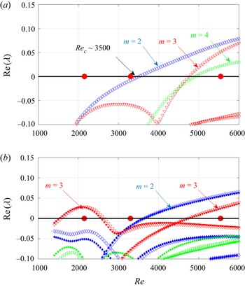


 Open access