


Introduction
Ice spikes have puzzled observers for decades. Published reports and theories go back to Reference DorseyDorsey (1921) and Reference BallyBally (1933). Since then, numerous reported observations have appeared (Reference BellBell, 1959; Reference HaywardHayward, 1966; Reference Krauz, Harron and LitvanKrauz and others, 1967; Reference ThainThain, 1985; Reference LoebeckLoebeck, 1986; Reference WhiddetWhiddet, 1986; Reference NishiyamaNishiyama, 1987; Reference LewisLewis, 1988; Reference ClarkClark, 1991; Reference TurnerTurner, 1991; Reference BjorbaekBjorbaek, 1994; personal communication from D. O’Dowd, 2003), as well as various explanations and discussions (Reference DorseyDorsey, 1948; Reference BlanchardBlanchard, 1951; Reference MaybankMaybank, 1959; Reference HallettHallett, 1960; Reference MorrisMorris, 1993; Reference PerryPerry, 1993, 2001; Reference AbrusciAbrusci, 1997), and, quite recently, a number of websites (http://www.physics.utoronto.ca/~ smorris/edl/icespikes/icespikes.html; http://www.its.calte-ch.edu/-atomic/snowcrystals/icespikes/icespikes.htm).
Nevertheless, little systematic research has been performed to determine, quantitatively, the conditions necessary for the development of ice spikes, or the details of their growth (Reference Mason and MaybankMason and Maybank, 1960; Reference WascherWascher, 1991; Reference Maeno, Makkonen and TakahashiMaeno and others, 1994). The companion paper in this issue (Reference Libbrecht and LuiLibbrecht and Lui, 2004) is one of few attempts to document the growth conditions of ice spikes in the laboratory. In this paper, we focus on the growth behaviour of ice spikes in ice-cube trays, using a combination of cold-room experiments and simple analytical modelling.
We use the term “ice spike” to refer to long, thin ice protrusions that emerge from a confined volume of partly or completely frozen water that has solidified from the outside in. Most reports of ice spikes have them protruding upward from horizontal surfaces such as ice cubes and small pools of water. However, similar features have also been seen on freezing water drops (Reference BlanchardBlanchard, 1951; Reference Mason and MaybankMason and Maybank, 1960), and natural icicles (Reference Maeno, Makkonen and TakahashiMaeno and others, 1994; see also Fig. 1).
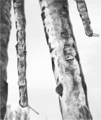
Fig. 1. Ice spikes near the tips of icicles hanging below a roof, observed by R. D. Sampson in Mansfield Center, Connecticut, 18 February 2003. The air temperature at the time of ice-spike growth was about -4.4°C.
Without complete confirmation of initiation and growth mechanisms, it is difficult to identify the necessary conditions and triggers for ice-spike growth. Reviewing the literature suggests that the following conditions appear to be of significance for ice-spike initiation and growth: air temperature, freezing rate (which is influenced by various factors, including air temperature, wind speed and relative humidity), container characteristics (shape, size, material, surface roughness, wall thickness), water impurities and vibrations. Reference Libbrecht and LuiLibbrecht and Lui (2004) have examined the influence of air temperature and salinity on the probability of ice-spike formation but there has been virtually no investigation of the other factors.
Methods
We used a 20 m3 Coldstream walk-in freezer for the experiments. In it, we were able to maintain a relatively constant air temperature, along with a presumably constant level of turbulence produced by the fans. Because of the size of the freezer, the thermal effects of opening and closing the door and observing the experiments were minimized. In a smaller setting, such as a home refrigerator freezer, opening a door to observe the growth could seriously disturb the freezing process by introducing additional turbulence, vibrations and sudden temperature changes.
Two types of container were used in the experiments: a blue commercial plastic ice-cube tray with stiffeners between compartments, and individual transparent Lexan containers of similar volume to the commercial tray compartments. In previous experiments and observations, commercial ice-cube trays available at local supermarkets have been successfully used to produce ice spikes on a regular basis (Reference WascherWascher, 1991). The commercial tray was stiffer than the Lexan tray. It was also different thermally, offering less exposure to the cold airflow than the Lexan tray. Each commercial tray contained 14 ice-cube compartments and was constructed with thin (< 2 mm) walls. The compartment dimensions in the commercial tray increased from 3.7cm × 2.1 cm at the base to 4.2 cm × 2.8 cm at the top with a depth of 2.3 cm, giving a filled volume of 22.3 mL. The Lexan tray had vertical walls and a flat bottom with dimensions 4.4cm × 2.9 cm × 3.0 cm and a filled volume of 38.3 mL. Affixed to it was a millimeter-scale grid to facilitate taking measurements from digital images. We thought that the transparent sides would aid in viewing the interior behaviour.
The ice-cube trays were supported on a wire rack during the experiments. The rack held the trays approximately 15 cm above the surface of a workbench. In this way, the entire surface of the trays was exposed to the turbulent air stream produced by the freezer’s cooling fans. This insured that freezing occurred from the outside in, leaving unfrozen liquid in the center of the ice cube.
The experiments were performed in three groups: the first used tap water in the commercial ice-cube tray, the second distilled water in the commercial tray, and the third distilled water in the Lexan tray. The City of Edmonton tap water was not tested for acidity, salinity or contaminants. The initial water-temperature range during experiments with the tap water was 27.0-44.3.°C. With the distilled water, the initial temperature range was 21.2-25.4°C. The range of initial water temperature was based on a recommendation by K. Wilkes (personal communication, 2003), who observed ice-spike growth in ice-cube trays only when the initial water temperature was 25-45°C. It is conceivable that colder water has enough dissolved air that the air bubbles formed on cooling allow room for ice expansion through compression of the gas, thereby reducing the volume of liquid available for ice-spike formation. All containers were filled to nearly full.
The air temperature in the freezer was measured with a copper constantan thermocouple. Measurements at 1s intervals were averaged over 1 minute and stored in a Campbell Scientific CR21X datalogger. The air temperature in the freezer was set at approximately -11.5°C, while the measured temperature fluctuated between -13°C and -10°C over approximately a 20 min period. The defrost cycle, which runs during a 90 min interval every 6 hours, resulted in a maximum temperature of -8.4°C and a minimum of-13.8°C. We tried to avoid experiments during the defrost cycle. Nevertheless, since ice-spike growth takes about 0.5 hours, the air-temperature range over a typical experiment was about 2°C, with a mean of-11 to -12°C.
The two cooling fans within the freezer created a weak, turbulent breeze (mean wind speed < 1ms-1) in the experimental area. No effort was made either to suppress or to enhance this ambient wind. Hence, we can say nothing about the impact of winds over the trays on ice-spike development, other than to observe that weak ambient winds do not appear to be a major inhibiting factor.
Water temperature within an ice-cube compartment was measured using a copper-constantan thermocouple on four separate occasions in three different positions along the vertical center line: slightly below the top surface, in the center of the compartment, and at the bottom. We did not make measurements at all three positions simultaneously since we were concerned that the thermocouples and their wiring might interfere with ice-spike formation. The thermocouple was placed into the water immediately upon inserting the ice-cube tray into the freezer. As with the air temperature, the water temperature data were stored as 1 min averages of 1s samples. Unfortunately, no ice spikes formed during any of the four temperature measurement experiments.
A tripod-mounted Canon PowerShot G3 (4.0 megapixel) digital camera was used to photograph the ice spikes. Using the macro setting, images of ice spikes at the highest resolution were captured at regular intervals, ranging from 10 to 60 s, during their growth. Scion Image software was used for digital measurements of the position of the tip and the diameter of the ice spikes as they evolved during growth, thereby allowing determination of the growth rate. We estimate that errors in the measured position information could result in a maximum growth-rate error of the order of 10%.
Results
Table 1 displays the results of38 experiments we performed using various water types and containers. Distilled water was much more conducive to producing ice spikes in a commercial ice-cube tray than tap water. Our probability of spike formation is in good quantitative agreement with Reference Libbrecht and LuiLibbrecht and Lui (2004) at a temperature of-11.5°C. That is to say, we observe a tap-water frequency of occurrence of 3.1%. Libbrecht and Lui suggest that medium-hard tap- water is equivalent to about a 10-3 mol L 1 solution of NaCl. Their figure 3 would suggest an occurrence frequency of 2.5-7.5% at this molarity and at -7°C. According to their figure 2, reducing the temperature to -11.5°C should reduce the occurrence probability to about 1.5-5%. Our value lies near the middle of this range.
Table 1. Ice-spike occurrence statistics

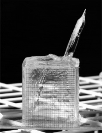
Fig. 2. Ice spike grown using distilled water in a Lexan container. Amillimeter-scale grid is affixed to the front surface of the container.
The Lexan container was somewhat less successful at producing spikes than the commercial ice-cube tray. This could possibly be the result of the thermal differences between the two containers. We suspect, however, that it may be the result of the fact that the Lexan container was somewhat less rigid than the commercial tray. This would provide greater room for expansion of the ice, thus making less liquid available for ice-spike formation.
An ice spike observed during an experiment with a Lexan container is shown in Figure 2. Other spikes were more tapered than this one. Some grew in several distinct stages with successively diminishing diameters. A high-resolution, time-lapse movie of the growth of a spike, made by animating the still images taken with the G3, can be viewed on the website of S. Morris (http://www.physics.utoronto.ca/-smorris/edl/icespikes/icespikes.html).
Three cases of ice-spike growth were analyzed using digital imaging software. Figure 3 shows the growth-rate variation with time for one of these cases, which is typical of the others. It is reminiscent of icicle growth behaviour. Initially, the growth rate is slow, but it accelerates to a maximum and this is followed by a sudden deceleration. Figure 4 shows how growth rate increases with decreasing tip diameter for the three cases combined.

Fig. 3. Ice-spike growth-rate variation with time. The plotted data were obtained by analysis of digital photographs of an ice spike grown in a Lexan container using distilled water. Other cases of ice-spike growth show similar growth-rate behaviour. The growth rate is plotted against elapsed time since the moment when distinct ice-spike growth was first observed. The diameter of the ice spike was not constant throughout its growth. The ice spike stopped growing after approximately 260 s. The data points are connected by a smooth curve to guide the reader’s eye. The experimental error in the growth-rate measurements is about ±0.00001 ms-1.

Fig. 4. Ice-spike growth rate as a function of ice-spike diameter for three cases combined. The ordinate is the growth rate in length (axially) while the abscissa is the diameter at the tip of the orifice. The error bars are estimates based on errors in the image analysis procedures. The two smooth curves are the theoretical growth rate calculated by combining Equations (2) and (3), where D is the thickness of the growing ice shell. D values of 0.0025 m and 0.0037 m are estimates, based on Equation (3), of the shell thickness after 30 and 45 min respectively. Distinct ice-spike growth was first observed between 30-45 min after the ice-cube tray was placed in the freezer, in all three cases.
Using small crystals of potassium permanganate, we confirmed that the ice spike is hollow. Crystals dropped on to the tip of a spike fell through the spike to rest in the unfrozen water in the container. It was also inferred using dye that there is often little flow of water down the outside of the spike during its growth.
The cooling rate of water within a Lexan compartment was determined using a copper constantan thermocouple. Figure 5 shows the cooling rate with the thermocouple junction placed near the center of the container. Note that in Figure 5 “cooling rate” is the actual rate of change of temperature, which is negative. When we refer to “cooling rate” increasing, we mean that the absolute value of the rate of change of temperature is increasing. For a system temperature above freezing, the cooling rate generally diminishes to zero at the freezing point, exhibiting a spike along the way at around 4°C. Once the system temperature drops below the freezing point, the cooling rate increases once again and then finally drops to zero as the system temperature reaches the air temperature.

Fig. 5. Cooling rate at the center of the Lexan container as a function of temperature at the same location. The cooling rate was determined by finite differencing the 1min average thermocouple temperatures. The data points are 1 min apart. Negative values imply heat loss from the water or ice. Time proceeds from right to left along the abscissa, as the system cools. A smooth curve has been added to guide the reader’s eye. The experimental error in the cooling rate is about ±5%.
We originally thought that good air circulation about the ice-cube trays might be an important factor in producing spikes. Hence the trays were placed on a wire mesh rack. However, one spike formed during a trial with the tray sitting on the particle-board surface of the workbench.
Interpretation of Cooling Curve
The cooling curve in Figure 5 exhibits several regimes. The results for the upper and lower positions of the thermocouple are qualitatively similar, although the measurements were made on separate occasions. Initially, there is a brief transient phase during which the cooling rate rapidly increases. This is probably the result of rapid surface cooling accompanied by convection, which allows the center to begin to cool. The transient is followed by almost linear behaviour reminiscent of a lumped capacity version of Newton’s law of cooling, in which the rate of cooling is proportional to the temperature difference between the water mass and its environment:
where m is total water mass, c w specific heat capacity of water, A water surface area, h effective total heat transfer coefficient and T a air temperature. Equation (1) lumps together the heat transfers due to evaporation from the upper surface, conduction through the container walls, convection to the air stream and longwave radiation. Not all of these are linearly dependent upon the air-water temperature difference, but a linear dependence can be a reasonable approximation if the temperature difference is not too large. In using Equation (1), we also assume that the water temperature field can be represented by a single value, the “system temperature”, T, which requires that the internal mixing processes should be efficient. Finally, we need to assume that the measured temperature in the very center of the container is representative of this system temperature. The system temperature is a bulk temperature or average temperature for the ice and liquid in the container.
At a temperature near 4°C, the cooling rate drops, then increases suddenly, finally dropping to zero at 0°C as latent heat is released. Once freezing is complete, the cooling rate rises from zero and then finally falls to zero again as the ice temperature reaches the air temperature. The behaviour near 4°C is possibly caused by a change in the internal convection regime, related to the fact that liquid water achieves its maximum density near 4°C. We suspect that, when the measured center temperature reaches 4°C, there is a transition from an upper convection cell overlying a lower stable layer to a lower convection cell underlying an upper stable layer. This could happen if the center temperature is higher than the temperature at both the upper and lower boundaries of the liquid. Unfortunately, we cannot explain why such a convective transition should give rise to a sudden increase in the cooling rate. Future experiments using flow tracers may help to answer these questions. The peak in cooling rate near -4°C is probably a result of the fact that, between 0°C and -4°C, some regions of the system remain unfrozen, with a temperature near 0°C, even though the measured center temperature is below freezing. The release of latent heat from these regions prevents the center from cooling as quickly as it would if the entire system were at the same temperature. Hence the cooling rate rises with time for a while and then eventually drops once the entire system has frozen. This illustrates the interpretational difficulty that arises when using a single temperature, the center temperature, to represent the entire system. It also suggests that, in future experiments, one should attempt to measure the temperature field in the container more completely.
Using the observed linear cooling rate, between about 16°C and 8°C, and the measured air temperature, it is possible to use Equation (1) to estimate the effective heat transfer coefficient. We determined a value of 37 W m-2 K-1. While its magnitude seems reasonable, this value must be treated with some caution, since the strict application of Equation (1) requires a Biot number, Bi <1, while in our case Bi ~1, based on internal conduction alone. However, convective stirring within the liquid may help to reduce the effective Biot number. The Biot number is a non-dimensional number expressing the ratio of internal conductive heat-transfer resistance to external convective heat-transfer resistance. A Biot number exceeding unity suggests that the resistance to internal heat conduction is greater than the resistance to external convection at the surface, and hence that internal temperature gradients cannot be ignored.
Simple Analytical Growth Model
It is possible to predict the growth rate of an ice spike if one assumes that its volumetric growth is entirely accounted for by the extrusion of liquid water from the interior of the container, as a solid ice shell of uniform thickness grows inward. We will make no allowance for dendritic growth or deformation of the ice cube and container walls. We will further assume that the ice spike has access to the entire unfrozen water supply within the container. A simple relation can then be derived by assuming the ice cube to be perfectly cubic of side H, and the ice spike to be a circular cylinder of length L and diameter d, measured perpendicular to the spike axis. If, at time t, the ice shell has grown to a thickness D, and the shell is continuing to grow inward at a rate dD/dt, then the growth rate of the ice spike may be expressed as:

where ρ w and ρ i are the density of water and ice respectively. The term 6(H – 2D)2 is just the instantaneous interfacial area between the water and ice. For non-cubic containers, it can be replaced by an appropriate expression for this area.
If the ice shell is thin, its growth equation may be written as (Reference Lozowski, Jones and HillLozowski and others, 1991):

where T f is the equilibrium freezing temperature, l f is the specific latent heat of freezing at T f and h is the heat-transfer coefficient for heat transport away from the phase boundary. Although we are not certain exactly where ice-spike growth might occur in Figure 5 since no spikes actually formed during this particular experiment, we have nevertheless used the value of the heat-transfer coefficient determined from Equation (1). Since ice spikes represent a relatively small fraction of the system mass, it is likely that the cooling-rate curves with ice-spike formation will be similar to Figure 5.
Combining Equations (2) and (3) allows us to estimate the growth rate of an ice spike. The dashed curves in Figure 4 are predicted ice-spike growth rates at 30 and 45 min after insertion of the container into the cold room. All of the ice spikes considered in Figure 4 grew during this interval. There is fair agreement with the observations. The significant discrepancy at the smallest diameter most probably occurs because freezing near the base of the spike eventually cuts off the liquid core of the spike from the liquid reservoir in the container. At this point, further growth results from extrusion of liquid from the much smaller liquid reservoir within the spike itself, leading to a lower growth rate.
Discussion
The process of ice-spike formation begins with the cooling of the liquid in the container. The data used to plot Figure 5 reveal that the center temperature dropped from 16.4°C to -0.2°C in 18 min following insertion into the cold room. It then remained at -0.2°C, with fluctuations of a few hundredths of a degree, for the next 114 min, after which it cooled to -10.0°C in a further 47 min. Although an ice spike did not actually occur during this experiment, spikes typically began to form, in other experiments, around 30-45 min after insertion into the cold room. This is early in the “constant temperature” phase, where the central temperature is slightly supercooled and ice needles have already been observed to form at the top surface and in the interior of the liquid. At this point, the ice thickness, were it uniform, would be only 2-3 mm, as suggested by Figure 4. Hence the ice is quite fragile at the onset of spike formation, suggesting that spikes are unlikely to be a high-pressure phenomenon.
Instead, ice-spike growth begins when a sessile liquid drop is extruded from a small unfrozen hole in the ice surface. The boundaries of the hole appear to be formed by several ice needles, which grow along the surface. The hole is typically triangular, presumably because the probability of two or three needles intersecting is greater than the probability of four or more intersections (two needles plus a container wall can form a triangular hole). We can merely speculate as to why the hole remains unfrozen. Reference HallettHallett#x2019;s (1960) explanation is that the c axis (optic axis) of each of the bordering needle crystals lies close to the surface. Hence the inward growth rate, towards the center of the hole, is slow. Such a requirement could explain why ice-spike formation has a stochastic component, since the crystallographic growth directions will be determined by whatever nucleates the needles. Once a hole of this type has been formed, the process becomes somewhat more deterministic, but crystallography continues to play an important role. Expansion due to freezing beneath the surface leads to extrusion of a liquid drop through the hole. The perimeter of the drop begins to freeze in the form of a thin ice shell, while the tip remains unfrozen as more liquid is extruded upward to renew the sessile drop. Surface tension tends to round out the initially triangular cross-section. Hence the ice spike is effectively a dynamic pipe that propagates upward as the water in it is pushed towards its upper, open end.
The structures that are most likely to be recorded as spikes are the fastest-growing ones. Such spikes occur when the length growth rate of the wall of ice is just fast enough that it keeps up with the rate of liquid extrusion into the sessile drop. Obviously the wall cannot grow faster than this or there would be no liquid for it to grow into. On the other hand, if the wall growth rate is too slow, the liquid tends to overflow and produce a “volcanic” cone rather than a spike. Such“volcanic” bumps on frozen ice cubes are actually quite common. The requirement for rapid upward wall growth is that the a-axis direction be nearly vertical. A necessary condition for this is that the c-axis direction be nearly horizontal. Hence the nucleation events that produce the unfrozen hole in the surface also help to determine whether or not a spike will form.
It is conceivable that a crystallographic explanation of ice-spike growth, such as we have suggested above, may also explain, at least qualitatively, Reference Libbrecht and LuiLibbrecht and Lui’s (2004) observation of a maximum in spike frequency at a temperature near -7°C. Near 0°C, the a-axis wall growth rate may not be sufficient to keep up with the rate of water extrusion, leading to volcanic cones but no ice spikes. On the other hand, at low temperatures, the c-axis growth rate may be high enough to close the surface hole before significant liquid extrusion can occur. This could lead to a build-up of internal pressure, causing internal cracking and a bulging of the ice surface but, again, no ice spikes. Ice-spike formation should therefore prevail at an intermediate temperature where the a-axis growth rate is a maximum and the c axis growth rate a minimum. Perhaps it is coincidental but, in growth from the vapour, such a situation prevails around – 6°C, very close to Reference Libbrecht and LuiLibbrecht and Lui’s (2004) observation of -7°C.
Once initiated, the ice-spike growth process continues until ongoing freezing of the spike wall near its base cuts off access to the liquid in the container. This cut-off can readily be observed. At this point, freezing of the liquid within the spike it self may give rise to a sequence of secondary spikes of successively smaller diameter. We have observed as many as two secondary spikes. Occasionally, the secondary spikes appear to freeze at both ends simultaneously, leading to a build-up of internal pressure and subsequent fracture.
Conclusions
As a result of these experiments, several extant hypotheses for ice-spike growth can be rejected. We saw no evidence for sublimative growth, for example. There was also no evidence supporting mechanical fracture of the ice shell, followed by sudden freezing of an emerging liquid jet. Rather our results support the Bally-Dorsey hypothesis, which predicts relatively slowly growing spikes with low water pressures and growth times of several minutes to tens of minutes. Our observations are also consistent with a formation mechanism that is dominated by crystallographic effects.
Numerous uncertainties remain regarding the growth mechanism of ice spikes. We do not, for example, understand what controls the onset time of ice-spike growth, the initial spike diameter, the growth angle and the tapering angle. Because of the stochastic effects alluded to above, it may be that these parameters are essentially unpredictable. It would be interesting to know if the larger spikes seen on bird-baths and elsewhere are also produced by the same mechanism. If so, our theory would suggest that they grow rather more slowly than spikes on ice cubes. We do not understand why some ice spikes seem to retain faceted walls (personal communication from D. O’Dowd, 2003) while most others develop a rounded cross-section. Perhaps, as Reference HallettHallett (1960) suggests, a faceted wall is an indication that the c axis is almost horizontal. Certainly a more thorough study, including flow visualization, that examines the crystal structure within an ice cube prior to, during and after ice-spike growth, is in order. While Reference Libbrecht and LuiLibbrecht and Lui (2004) have established the effects of salinity and air temperature, the possible influence of dissolved air should be further explored, along with the influence, if any, of wind speed and direction, compartment shape and size, initial water temperature and vibrations.
Acknowledgements
The senior author (Hill) is grateful for the award of an Undergraduate Summer Research Assistantship from the Natural Sciences and Engineering Research Council of Canada (NSERC), while the participation of the junior authors (Lozowski and Sampson) was made possible through an NSERC Discovery Grant to Lozowski. We wish to thank T. Forest and the Mechanical Engineering Shop, University of Alberta, for fabricating the Lexan trays and reviewing the manuscript. J. Wilson kindly provided a data logger and helpful experimental advice. S. Morris, University of Toronto, offered us inspiration and a lot of clues through his website and paper referenced below. Many thanks to K. Wilkes andJ. Melenko, whose ice-spike experiments in 1992 as part of Lozowski’s cloud physics course set the stage for the present work. Finally, thanks to W. Weekes and C. Knight for their reviews, which forced us to think hard about the problem.


