


Background
The last few years have seen exponential growth in the use of cryo-electron microscopy (cryo-EM) by structural biologists. In 2013, only seven cryo-EM density maps were deposited at the Electron Microscopy Data Bank (EMDB, www.emdatabank.org) at resolutions better than 4 Å, but as of March 2020, over 2000 density maps have been deposited with resolutions better than 4 Å. The vast majority of these maps have also been of a quality that is good enough to be interpreted in terms of an atomic model of the constituent proteins and related macromolecules. Cryo-EM methods can thus be clearly viewed on par with other experimental approaches, such as X-ray crystallography and nuclear magnetic resonance spectroscopy, in terms of their potential for atomic-resolution structure determination.
Structure determination by cryo-EM involves numerous experimental and computational steps, but the prohibitive cost of purchasing, maintaining, and operating state-of-the-art microscopes remains a major barrier to using these methods to advance the study of biological mechanisms. Recognizing this need, the National Cancer Institute (NCI) launched the National Cryo-EM Facility (NCEF) in May of 2017 as a federally funded pilot effort to begin meeting the needs of cancer researchers in United States academic labs who do not have adequate access to these instruments. The goal of the facility is to provide rapid access to users at no cost and with a simplified access model.
Our intention in compiling this summary of the NCEF is three-fold. The first aim is to present a standardized method for data collection, enabling accurate citation by users when publishing structures based on data generated at the NCEF. Second, we note observable trends in parameters that appear to be predictive of success in achieving higher resolution based on >350 data collection sessions at the NCEF since its launch (see Figure 1 for some representative structures published using data collected at NCEF). Third, we present a description of our operational procedures that could potentially serve as a reference point for other newly launched cryo-EM user facilities that wish to adopt a similar model for user access.

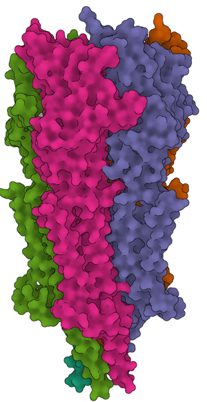
Figure 1: Examples of structures solved with the help of data collection at the NCEF. (a) 5-HT3A serotonin receptor in complex with serotonin [Reference Basak8]. (b) Gasdermin A3 membrane pore [Reference Ruan9]. (c) Active Dot1L nucleosome complex [Reference Worden10].
Access to NCEF
NCEF resources are accessible to any United States researcher from a non-profit organization. There is no cost for access, and there is no prerequisite for prior NCI or NIH funding. Users are not required to provide a research proposal but are required to state that their project is cancer-related, which admits a relatively broad scope of projects given that a large number of basic questions in cell biology are relevant to cancer research. Researchers contact the NCEF by sending a submission form (“Sample Information Form” [SIF] available at https://www.cancer.gov/research/resources/cryoem/access) along with screening images from their grids. If the screening images indicate that the user's grids are of a quality adequate for data collection, the application is approved, typically within 24 hours after submission of the application. When the images are deemed to be inadequate to meet standards for data collection at the NCEF, more information might be requested from users, or the NCEF staff will engage with users to help improve sample quality. Once the request is approved, the frozen samples are shipped to the NCEF, and the project enters a scheduling queue once samples are received. The various stages of user engagement with the NCEF are schematically summarized in Figure 2.

Figure 2: General schematic of the workflow that a user experiences when interacting with the NCEF. 1) The user purifies their protein of interest. 2) The user optimizes freezing conditions for their grids. 3) The user screens grids for quality and sample concentration on a cryo-electron microscope. 4) If screened images are of low quality (damaged grid, thick ice, and/or low sample concentration), the user starts over at either steps 1 or 2 depending on the nature of the problem. 5) If screened grids are of high quality (intact grid, thin ice, and high sample concentration), then the user proceeds with submission. 6) The user fills out a Sample Information Form (SIF) and submits it to the NCEF for review. 7) The SIF is reviewed by NCEF staff, which is either approved within 24 hours or sent back with suggestions on what needs to be done for the submission to be approved. 8) If the sample is approved, the user sends frozen grids to NCEF in an approved dry shipper with grid inventory and return shipment label enclosed. 9) Prior to imaging, NCEF staff makes contact with users to determine imaging parameters, usually via an online video conference. 10) After the imaging session has been completed, the user is able to download their images from the NCEF's Globus endpoint and receives a detailed report by email.
Because samples are not scheduled for a specific date, the queue at NCEF is dynamic and can adapt rapidly to any delays. Users are encouraged to ship their samples by mail rather than visit in person so that the need for coordination of microscope operations with travel schedules can be minimized. Data runs are set up with the users, directly engaged via video conferencing. Remote access to a monitoring website, providing on-the-fly feedback on imaging during the run, is available to users and NCEF microscopists. To minimize wait time, only one user project from each principal investigator's lab is in the active queue at any one time, and data collection is restricted to 48 hours, unless technical problems with the microscope lead to significant loss (>4 hours) of data collection time.
Data Collection and Transfer Process
A typical 48-hour user session starts with transfer of grids into the microscope and screening of each grid for 10–15 minutes to determine the amount of area that can be imaged and to check the quality of particle projection images. This is followed by checking column alignment, including gun and condenser alignment, and collection of a fresh gain reference for the detector. Following these steps, a video conference is initiated with the user to discuss targeting and imaging parameters. Once imaging parameters are set, an automated data collection run is set up, and a sufficient number of target areas are selected to sustain approximately 40 hours of data collection. For quality-control purposes, data quality is analyzed concurrently with data collection using Scipion software [Reference de la Rosa-Trevín1], by MotionCor2 [Reference Zheng2] and CTFFind4 [Reference Rohou and Grigorieff3], and the results are streamed to a website that can be accessed by the users. At the end of data collection, the data are compressed and transferred to a storage server where they can be downloaded by the users through the Globus GridFTP client. A full report is sent to each user with information on how to download the data. This report includes all the imaging settings, comments and recommendations on grid and sample quality, and the results from the quality-control analysis. Roughly one month after data collection, the NCEF submits a questionnaire to each user to receive feedback on the data collection process and the quality of the data.
Methods
Cryo-EM data collection.
Vitrified grids are imaged using a Titan Krios transmission electron microscope (Thermo Fisher Scientific) at 300 kV equipped with a K3 direct electron detector and Quantum energy filter (both from Gatan Inc.) with a slit width of 20 eV. Data are typically collected with a 100 nm C2 aperture and no objective aperture. Data are usually collected with an unbinned pixel size of 0.85–1.3 Å, a total electron dose between 40–60 e−/Å2, and a defocus range of -1.0 to -2.5 µm. Common camera setups use an imaging dose rate of 14–20 e−/px/s on the K3 camera (2–8 e−/px/s on the K2 camera). Automated data collection is performed using Latitude S software from Gatan Inc. To minimize beam tilt distortion, which Latitude S does not currently correct for, image shifts are set up over short distances of less than 2 µm when multiple images are collected following the move of the stage to a given position. The precise settings for data collection vary according to user requests and requirements.
Determination of ice thickness from a single image.
Electrons passing through a vitreous ice layer may experience either elastic or inelastic scattering. Without an objective aperture, few scattered electrons have scattering angles large enough to prevent them from contributing to the final image. An objective aperture can be used to block out electrons with the largest scattering angles, thus increasing image contrast. An energy filter can block almost all inelastically scattered electrons (which only contribute noise to an image) and consequently increase the signal-to-noise ratio in the image. The amount of scattered electrons is also proportional to the ice thickness and can be described as follows:

with t being the ice thickness, Λ the inelastic mean free path, I 0 the unfiltered intensity of the beam, and I zlp the filtered intensity. In principle, Λ is dependent only on voltage and the composition of the sample, but in more practical settings some elastically scattered electrons are also filtered in the optical path through the electron microscope, specifically when an objective aperture is used. In such cases Λ cannot be described purely as inelastic mean free path and is also dependent on the optical path and particularly on the size of the objective aperture.
Determining both the unfiltered and filtered intensity on each data position is a generally accepted way of measuring the ice thickness [Reference WJ4], but it increases the time per image during data collection. However, it is possible to simplify the process on the Krios because the optics on the Krios are such that very few scattered electrons are eliminated without an objective aperture and the energy slit on the energy filter. This means that the unfiltered intensity is very close to the intensity of the electron beam without a sample, and in this case we can neglect the difference and change (1) to:

With I tot the intensity of a beam without sample, D tot the total electron dose on the sample and D image the dose measured on the image. This assumption is only correct for weakly scattering samples like thin ice and carbon films. It does not hold for very thick films (>>200 nm) or other strongly scattering material films (for example, gold foil). To determine average ice thickness for each image from the average dose (and the known total dose during the session), one must determine Λ on the system at conditions close to standard single-particle imaging conditions. Λ was measured to be 250 nm according to the method described by [Reference Angert5] and [Reference Feja and Aebi6]. With the measured value Λ, Equation (2) can be used to determine the average ice thickness of each image in an imaging session using the dose per pixel (or per Å2) measured from the image. The value of D tot is measured carefully before each data collection and specifically set to a particular value (standard is 40 or 50 e/ Å2). In our experience, beam stability on the Titan Krios is excellent, and D tot does not change significantly (<1%) during a 2–3 day run.
Effect of Ice Thickness on Data Quality
Since ice thickness seems to be a very important factor to determine data quality, it should be strongly considered when optimizing plunging conditions and screening grids. The visual appearance of the “vitreous ice ring” in the image FFT, the broad diffraction peak corresponding to distances of water molecules in vitreous ice, is dependent on ice thickness. This can be used as a rough rule of thumb. As can be observed in Figure 3, in ice that is thinner than ~50 nm, no vitreous ice ring is observed in the power spectrum, whereas with ice thickness >50 nm, the ring becomes progressively more prominent in the power spectrum.

Figure 3: Power spectra provide approximate guidelines for estimating ice thickness. Examples are shown for power spectra of different images collected from a single NCEF imaging session. The average ice thickness of the corresponding images is given in the top right of each power spectrum. The vitreous ice ring at about 0.39 Å (marked with a white arrow in the bottom right image) becomes progressively more visible as the ice thickness in the sample increases. Only in vitreous ice thicker than ~50 nm is the ring clearly visible.
The thickness of ice can sometimes vary widely within a single grid, as shown in an example presented in Figure 4A. The information limit is also determined by ice thickness, with thinner regions producing images with information extending to higher resolution (Figure 4B) [Reference WJ4]. As users have shared results obtained from data collected at NCEF, a measurable trend has emerged that correlates resolution with ice thickness. Specifically, thinner ice strongly correlates with higher reported resolutions (Figure 4C). Interestingly, there was no obvious correlation between the extent of motion in the movie frames and the reported resolution (Figure 4D), indicating that the software for motion correction available to most users is sufficient enough to compensate for beam-induced and stage motion that occurs during data collection.

Figure 4: Effect of ice thickness on data quality: (a) Ice thickness distribution for a single NCEF imaging session. (b) CTFFIND4 resolution limit versus ice thickness for each image in the same imaging session. We find that ice thickness is usually a good predictor for resolution limits (as determined by CTF fitting with CTFFIND4), with only images that have ice thinner than ~50 nm resulting in achieved resolutions between 3 Å and 4 Å. (c) User-reported resolution values versus average ice thickness of the corresponding imaging session for a subset of the imaging sessions where ice thickness measurements were carried out. (d) User-reported resolution versus average motion between frame 1 and frame 2 of the corresponding imaging session. While ice thickness values show strong correlation with reported resolution, no obvious correlation is observed between average motion and the reported resolution.
Summary and Future Perspective
Since its inception in May 2017, the NCEF has executed over 350 data collection runs, providing services to 72 investigators in 39 institutions (Figure 5), operating at an overall uptime of >90%. Operations between May 2017 and February 2020 were carried out with a single Titan Krios microscope, but as of April 2020, the facility will operate with two Titan Krios microscopes, each equipped with Falcon 3EC and GIF/K3 cameras. Automated imaging on the K3 cameras is performed using either Latitude S (Gatan, Inc.) or SerialEM software [Reference Mastronarde7], whereas collection on the Falcon 3EC is performed with EPU (Thermo Fisher Scientific). The average size of data collected per session increased from under a terabyte to several terabytes as we transitioned from a K2 to K3 camera, but the overall trends in data size (Figure 6) help us anticipate requirements for data storage. As we look ahead to the coming years, we foresee that biologists with minimal cryo-EM or structural biology experience will likely constitute the dominant user community. We therefore anticipate enhancing our services to offer progressively more advanced feedback by providing image processing results so that users can quickly assess the feasibility of obtaining useful 3D structures from the data collected at the NCEF.

Figure 5: Monthly (orange) and cumulative (blue) imaging sessions at the NCEF. Logos for all participating user institutions are shown above. The data show that the microscope averages ~10 imaging sessions per month.

Figure 6: Data collection results from earlier data collection runs that used the K2 summit camera (orange circles) and later data collection runs that used the K3 camera (blue triangles). (a) The total number of movies collected in each imaging session depends on imaging strategy (image shift or stage shift) and on the actual imaging time (standard 48-hour runs or the occasional 72-hour runs on some weekends and holidays). (b) shows the total compressed size for each imaging session. The total compressed size depends on the number of movies, but also on the use of the super-resolution mode for data collection.
Acknowledgments
This project has been funded in whole with Federal funds from the Frederick National Laboratory for Cancer Research, National Institutes of Health, under contract HHSN261200800001E. The content of this publication does not necessarily reflect the views or policies of the Department of Health and Human Services, nor does mention of trade names, commercial products, or organizations imply endorsement by the US Government.


