


Introduction
Multitemporal satellite imagery and older aerial photography have been used extensively in the last decade to quantify glacier changes in mountainous areas throughout the world, including Patagonia (Reference Aniya, Sato, Naruse, Skvarca and CasassaAniya and others, 1996), the Swiss Alps (Reference Kääb, Paul, Maisch, Hoelzle and HaeberliKääb and others, 2002; Reference Paul, Kääb, Maisch, Kellenberger and HaeberliPaul and others, 2002), central Asia (Reference Khromova, Dyurgerov and BarryKhromova and others, 2003, Reference Khromova, Osipova, Tsvetkov, Dyurgerov and Barry2006; Reference Surazakov and AizenSurazakov and Aizen, 2006; Reference Aizen, Kuzmichenok, Surazakov and AizenAizen and others, 2007; Reference BolchBolch, 2007), the Peruvian Andes (Reference GeorgesGeorges, 2004; Reference Silverio and JaquetSilverio and Jaquet, 2005) and the Himalaya (Reference Kulkarni and BahugunaKulkarni and Bahuguna, 2002; Reference Kulkarni, Rathore, Mahajan and MathurKulkarni and others, 2005). More recently, satellite images have been used to estimate glacier mass balances and equilibrium-line altitudes (ELAs) (Reference Khalsa, Dyurgerov, Khromova, Raup and BarryKhalsa and others, 2004; Reference Rabatel, Dedieu and VincentRabatel and others, 2005; Reference Berthier, Arnaud, Kumar, Ahmad, Wagnon and ChevallierBerthier and others, 2007). There is continued interest in mapping the world’s glaciers using satellite data. The Global Land and Ice Measurements from Space (GLIMS) project was initiated with the goal of mapping the world’s glaciers using satellite imagery (Reference KargelKargel and others, 2005). Remote-sensing methods are useful for detecting glacier changes in a timely manner in remote regions where traditional field-based glaciological methods are limited by difficult logistics and lack of support.
Tropical glaciers of the Cordillera Blanca, Peru, are of interest for several reasons. At local scales, glacier runoff constitutes the main water source for hydropower generation, irrigation for agriculture use, and domestic or animal consumption. Rapid melting of Andean glaciers in recent decades (Reference Kaser, Juen, Georges, Gomez and TamayoKaser and others, 2003) poses a threat to local water resources. There is also concern about glacier-related hazards such as glacier lake outburst floods (GLOFs) associated with moraine-dammed lakes. An extensive glacier inventory for the Cordillera Blanca was compiled on the basis of 1970 aerial photography (Reference AmesAmes and others, 1989). More recent Landsat Thematic Mapper (TM) and Système Probatoire pour l’Observation de la Terre (SPOT) satellite imagery was used to estimate changes in glacier extents at different time-steps (Reference Kaser, Georges and AmesKaser and others, 1996; Reference GeorgesGeorges, 2004; Reference Silverio and JaquetSilverio and Jaquet, 2005). Glacier lengths and mass balance have been reported for a limited number of glaciers with field measurements (Reference Hastenrath and AmesHasternath and Ames, 1995; Reference Ames and HastenrathAmes and Hasternath, 1996). However, there remains a paucity of information on glacier parameters such as glacier area, length, terminus elevations, hypsography, ELA, accumulation-area ratio (AAR), mass balance and hypsometry, due to a lack of reliable elevation data from which these parameters can be extracted. Furthermore, the relationship between glacier parameters and glacier area changes has not been investigated thoroughly in the Cordillera Blanca. Only one study (Reference Mark and SeltzerMark and Seltzer, 2005) evaluated the spatial distribution of glacier fluctuations with respect to climate forcing in the Andes.
The availability of new remote-sensing platforms with high spatial and temporal resolution, global coverage and reasonable financial costs provides the potential to evaluate glacier parameters in remote areas such as the Andes. Updated glacier parameters are needed to assess spatial patterns of glacier changes and their connections with climate fluctuations at local and regional scales. This study combines data from SPOT with field measurements and Geographic Information Systems (GIS) to understand spatial patterns of glacier fluctuations in the Cordillera Blanca at decadal scales. Specific objectives include (1) estimating the glacierized area in 2003, (2) estimating changes in glacier area from 1970 to 2003, (3) estimating changes in the elevations of glacier termini over the same time-span, (4) quantifying hypsometry changes and (5) evaluating air-temperature and precipitation trends in the last 30 years.
Study Area
The study area is the Peruvian Cordillera Blanca (Fig. 1), the largest glacierized area in the tropics, stretching 180 km north–south between 8°30′ S and 10° S (Reference Kaser, Ames and ZamoraKaser and others, 1990). The glacierized area was estimated to be 723.37 km2 based on 1970 aerial photography, with an average thickness of 31.25 m (Reference AmesAmes and others, 1989). The Cordillera Blanca comprises valley glaciers with elevations ranging from ∼3000 to ∼6800 m and very steep slopes. Some of the glacier tongues are covered with debris, and many of them terminate at moraine-impounded glacier lakes. Climatically, the Cordillera Blanca is situated in the outer tropics, characterized by an absence of thermal seasonality and a distinct seasonality of precipitation, with one distinguishable wet season (austral summer) and one dry season (winter) (Reference Kaser and OsmastonKaser and Osmaston, 2002). Snow accumulation occurs during the wet season, and there is relatively little accumulation in the dry season. Ablation occurs year-round, with higher rates in the wet season (Reference Kaser and OsmastonKaser and Osmaston, 2002). Southeasterly winds bring precipitation from the Amazon basin, making the windward (eastern) side of the cordillera two to three times wetter than the leeward (western) side (Reference Johnson and SchwerdtfegerJohnson, 1976).

Fig. 1. Cordillera Blanca study area. Spatial domain 1 is the area covered by the two orthorectified SPOT scenes from August 2003. Also shown are ground-control points acquired in the field (white stars), and climate stations with complete 30 year temperature and precipitation records (white squares).
Methods
Data sources
The baseline dataset for this study was the 1970 glacier inventory for the Cordillera Blanca, constructed from aerial photography and published by Reference AmesAmes and others (1989). We obtained the digital version of the inventory from Unidad de Glaciología y Recursos Hídricos (UGRH) of Instituto Nacional de Recursos Naturales Ancash (INRENA), Peru. In 2004, we acquired 24 ground-control points (GCPs) on non-glaciated terrain (road intersections, curves and buildings visible on the satellite images) using an Ashtech ProMark2 differential global positioning system (DGPS). The horizontal and vertical accuracy of the GPS points after post-processing was <1 m. These GCPs were used for orthorectification of the satellite scenes and validation of the digital elevation data. We constructed a digital elevation model (DEM) with 30 m cell size by interpolating contour lines digitized from two 1 : 100 000 topographic maps based on 1970 aerial photography, using the TOPOGRID algorithm (Reference Burrough and McDonnellBurrough and McDonnell, 1998). We denote this DEM as the ‘1970 DEM’. The methodology was tested at a different site in Peru and was found to yield satisfactory results (Reference Racoviteanu, Manley, Arnaud and WilliamsRacoviteanu and others, 2007). We estimate the horizontal accuracy of the DEM to be less than half the contour interval (25 m). Its vertical accuracy (root-mean-square error in the vertical coordinate (RMSE z ) with respect to the GCPs) is 18 m. All the datasets were projected to Universal Transverse Mercator (UTM) zone 18S, with the World Geodetic System 1984 (WGS84) horizontal datum and the Earth Geopotential Model 1996 (EGM96) vertical datum.
The SPOT5 sensor launched in 2002 acquires data in multispectral and panchromatic mode, suitable for glaciological applications. Bands 1 (0.50–0.59 μm) and 2 (0.61–0.68 μm) of SPOT5 are in the visible part of the electromagnetic spectrum (VIS), band 3 (0.79–0.89 μm) is in the near-infrared (NIR) and band 4 is in the mid-infrared (MIR) (1.58–1.75 μm). The spatial resolution of the sensor is 10 m for the VIS and NIR bands and 20 m for the MIR. Two scenes were needed to cover about 90% of the Cordillera Blanca. The scenes were acquired in August 2003, at the end of the dry season to ensure minimal snow cover, and had no cloud cover. The scenes were orthorectified using the field-based GCPs and the DEM using Toutin’s model (Reference Toutin, Chénier and CarbonneauToutin and others, 2002). The horizontal root-mean-square error (RMSE x , y ) with respect to GCPs was <5 m for both images, which is considered appropriate as it is half of the SPOT5 image pixel size.
Long-term changes in annual temperature and precipitation were evaluated from climate records provided by Servicio Nacional de Meteorología e Hidrología (SENHAMI), Peru. Climate stations are located on the western side of the Cordillera Blanca; there are no long-term climate records from the eastern side (Fig. 1). We selected climate stations based on two criteria: (1) continuous and complete long-term records of 30 years, from 1970 to 1999; and (2) representation of an elevation gradient from 3000 to >4000 m (Table 1). We evaluated the statistical significance of temperature and precipitation trends and determined the linear slopes for significant trends using the Mann–Kendall non-parameteric test (Reference Del Río, Fraile, Herrero and PenasDel Río and others, 2007).
Table 1. Climate stations with complete records from 1970 to 1999 (Fig. 1), with parameters measured, and the total changeover the 30 year period. Temperature and precipitation trends for the 1970–99 period for the different elevations are based on the Mann–Kendall non-parametric test

Glacier delineation and analysis
We tested various image classification techniques such as single-band ratios and ratio images with various band combinations, as well as unsupervised classification techniques (ISODATA) and supervised techniques (maximum likelihood classification). The normalized-difference snow index (NDSI) method (Reference Hall, Riggs and SalomonsonHall and others, 1995) proved to be superior to other band combinations based on visual inspection of color composites. The NDSI is a robust, easily applied method and is less sensitive to illumination variations than non-ratio techniques. The technique is similar to the normalized-difference vegetation index (NDVI) used for vegetation mapping and is calculated as (VIS − NIR)/ (VIS + NIR). It takes advantage of the high brightness values of snow and ice in the visible wavelengths (0.4–0.7 μm) vs low brightness value in the near and mid-infrared (0.75–1.75 μm) to separate them from darker areas such as rock, soil or vegetation. The NDSI is also useful to discriminate clouds if the 1.6–1.7 μm band is available (band 4 of SPOT), because at these wavelengths, clouds are reflective and snow/ice is absorbing (Reference DozierDozier, 1984). Band 4 was resampled to 10 m to match the resolution of the visible bands, using a bilinear method. The resulting NDSI image with values from −1 to 1 was segmented using a threshold value of 0.5 to obtain a binary map of glacier/non-glacier areas. Debris-covered glaciers were digitized manually using a slope map derived from the DEM and a color composite map (SPOT 234). The raw ice polygons were visually checked for classification errors such as persistent seasonal snow, rock outcrops and moraines. Ice divides were computed using watershed delineation commands, following the protocol of Reference Manley, Williams and FerrignoManley (in press). Resulting ice divides were visually inspected and refined manually, based on a shaded relief map constructed from the 1970 DEM.
To separate the ice mass into glaciers, we used the GLIMS definition of a ‘glacier’ tailored to remote sensing, compliant with the World Glacier Monitoring Service (WGMS) standards (B.H. Raup and S.J.S. Khalsa, http://www.glims.org/MapsAndDocs/assets/GLIMS_Analysis_Tutorial_a4.pdf). Under these standards, the bodies of ice above the bergschrund that are connected to the glacier are considered part of the glacier, as they contribute snow (through avalanches) and ice (through creep flow) to the glacier mass (Raup and Khalsa, http://www.glims.org/MapsAndDocs/assets/GLIMS_Analysis_Tutorial_a4.pdf). We excluded exposed rock, including nunataks and snow-free steep rock walls, from the glacier area calculations. Each glacier was assigned an ID based on its geographic location (latitude and longitude coordinates). Glacier fragments that separated from a main ‘parent’ glacier from 1970 to 2003 were assigned a single ID of that parent glacier to facilitate subsequent comparison with the 1970 inventory. The resulting polygons were coded as ‘internal rock’, ‘glacier boundary’, ‘proglacial lakes’, ‘supraglacial lakes’ and ‘debris boundary’ following specifications of Raup and Khalsa (http://www.glims.org/MapsAndDocs/assets/GLIMS_Analysis_Tutorial_a4.pdf). The accuracy of the SPOT-derived glacier outlines was computed using the ‘Perkal epsilon band’ and implemented as a buffer operation in vector GIS (Reference Perkal and NystuenPerkal, 1966; Reference Burrough and McDonnellBurrough and McDonnell, 1998). This method was shown to slightly overestimate the error (Reference Hoffman, Fountain and AchuffHoffman and others, 2007). Digitizing errors and ‘sliver’ polygons arising from overlay operations in mismatch areas (Reference Burrough and McDonnellBurrough and McDonnell, 1998) were eliminated manually. Confusion between shadowed glacier areas and internal rocks was eliminated by comparing these areas against the high-quality 1 : 100 000 Alpenvereinskarte Cordillera Blanca (Reference Moser, Georges and SchimmerMoser and others, 2000), to minimize classification errors. The SPOT5 glacier outlines were assigned positional accuracies and ingested in the GLIMS glacier database (http://nsidc.org/glims) maintained at the US National Snow and Ice Data Center (NSIDC) in Boulder (A.E. Racoviteanu and Y. Arnaud, http://www.glims.org).
The analysis of glacier changes was conducted at different spatial scales, so that we could compare our results with those of other investigators. The spatial domains, with their extents and characteristics, are shown in Table 2. Spatial domain 1 includes glaciers encompassed by the two SPOT scenes (Fig. 1). The two northernmost groups Rosco and Pelegatos) and two southernmost groups (Pongos and Caullaraju) were outside the two SPOT images and were not included in this domain. We first compared the 2003 SPOT-derived glacier outlines with the 1970 inventory for this domain to derive changes in glacier area, glacier terminus elevations and glacier median elevations. We constructed glacier hypsographies from the 1970 and 2003 outlines using elevations extracted from the 1970 DEM for both datasets. For each glacier in spatial domain 1, we calculated its area, terminus elevation, maximum elevation, median elevation, average slope angle and average aspect using grid-based modeling and zonal functions. Glaciers that broke into different parts were counted and analyzed as part of the same ‘parent’ glacier.
Table 2. The spatial domains used for analysis, with their characteristics

Spatial domain 2 is a subset of spatial domain 1 comprising 367 glaciers covering about 71% of the glacierized area, selected based on: (1) ice divides in 2003 matching closely those from the 1970 inventory; (2) glacier area greater than a cut-off value of 0.01 km2, which eliminated very small glaciers; and (3) minimal debris cover on glacier tongues. We investigated changes in glacier area from 1970 to 2003 and correlated these changes with glacier parameters using GIS methods and univariate statistics. The analysis of glaciers in spatial domain 1 was conducted separately for glaciers on the eastern and western sides of the Cordillera Blanca.
Spatial domain 3 is the total glacierized area covered by the 1970 Institut Géographique National (France) (IGN) inventory (Reference AmesAmes and others, 1989), and corresponds to our spatial domain 1 plus the four mountain groups at the northern and southern edges of the SPOT scenes (Fig. 1). To estimate the area of those glaciers outside the SPOT imagery in 2003, we used the recession technique developed by Reference Kaser, Georges and AmesKaser and others (1996) and Reference GeorgesGeorges (2004). The overall factor of recession calculated as Area2003/Area1970 was derived from spatial domain 1 and applied to the missing mountain groups.
Results and Discussion
The SPOT5 glacier inventory: spatial domain 1
The classification of the two SPOT5 satellite images in 2003 yielded 485 glaciers, covering an area of 516.1 km2. Out of these, 57 glaciers had debris-covered tongues, totaling an area of 14.9 km2, which is 3% of the total glacierized area. Descriptive statistics for the 485 glaciers derived from SPOT imagery are presented in Table 3. Elevations of the glacier termini range from 4204 to 5369 m, with a mean of 4881 m. On average, glacier termini are 102 m higher on the western slope of the Cordillera Blanca (4914 m) than on the eastern slope (4812 m) (Table 4). The median elevation of glaciers in spatial domain 1 ranges from 4420 to 5695 m, with an average of 5150 m (Table 3). Glaciers on the western side of the Cordillera Blanca have median elevations 116 m higher than those on the eastern side (Table 4). The median elevation of glaciers decreases from southwest to northeast, a trend represented by a tilted surface, oriented towards the northeast. This southeast–northwest trend in glacier termini and median elevation reflects the orographic effect of the Cordillera Blanca, and is consistent with the regional gradient noted in previous studies (Reference Kaser and GeorgesKaser and Georges, 1997). On the eastern side, increased precipitation due to orographic uplift from the Amazon basin favors the extension of glacier termini to lower elevations and induces lower ELAs (Reference Kaser and GeorgesKaser and Georges, 1997).
Table 3. Comparison of IGN 1970 and SPOT 2003 glacier inventories for spatial domain 1. Glacier elevations are based on the 1970 DEM for both the IGN 1970 and SPOT 2003 datasets
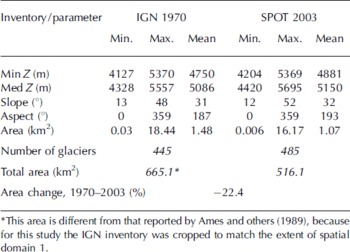
Table 4. Comparison of glacier parameters on the eastern vs the western side of the Cordillera Blanca (CB) for the glaciers in spatial domain 1

SPOT-derived glaciers range in size from 0.006 to 16.17 km2, with a mean size of 1.07 km2 (Table 3). There are only five glaciers with area smaller than 0.01 km2, which are remnants of larger glaciers. The frequency histogram of glacier area (Fig. 2) shows the non-linear decrease in the number of glaciers with glacier size, suggesting that small glaciers (<1 km2) are much more common than large glaciers (>10 km2). For example, 73% of glaciers are smaller than 1 km2, and 48% of glaciers are smaller than 0.3 km2. The Cordillera Blanca may be particularly sensitive to small changes in climate because of the large number of small glaciers.

Fig. 2. Area frequency distribution of the 485 glaciers in spatial domain 1 of the Cordillera Blanca, derived from the analysis of SPOT5 images. Glaciers smaller than 1 km2 are prevalent in this area.
On average, glaciers on the eastern side of the Cordillera are slightly larger than those on the western side (Table 4). There is a negative correlation between terminus elevation and glacier area (r = −0.6): larger glaciers tend to extend down to lower elevations, while smaller glaciers have higher termini. These patterns were observed in other glacier areas (e.g. Alaska Brooks Range (Reference Manley, Williams and FerrignoManley, in press) and the Swiss glaciers (Reference Kääb, Paul, Maisch, Hoelzle and HaeberliKääb and others, 2002)).
The average slope of the glaciers in spatial domain 1 is 32° (Table 3), with an almost normal distribution (Fig. 3). The average glacier orientation is 193° (southwest) (Table 3), with 32% of the glaciers oriented towards the south and southwest (Fig. 4). These results are similar to the Reference AmesAmes and others (1989) inventory from 1970, which reported an average orientation of 187° (Table 3). In the outer tropics of the Southern Hemisphere, these aspects are more shaded in the day during the wet (accumulation) season (Reference Mark and SeltzerMark and Seltzer, 2005). Hence, the net energy balance is likely lower on southwest-facing aspects during the wet season, favoring precipitation as snow compared to rain, and reducing ablation from sublimation and melt.

Fig. 3. Slope frequency distribution of the 485 glaciers in spatial domain 1. On average, glaciers in this area are steep, with a mean slope of 32°.

Fig. 4. Aspect frequency distribution of the 485 glaciers in spatial domain 1. Numbers represent the percent of glacier area in 22.5° aspect bins. Glaciers in the Cordillera Blanca have a southwest preferred aspect.
The comparison of glacier statistics for the 1970 and 2003 inventories (Table 3) points to some changes in glacier parameters in spatial domain 1. The digital version of the 1970 IGN inventory covered an area of 665.1 km2. The SPOT-derived glacier area was 516.1 km2 in 2003, indicating a loss in glacier area of ∼22.4% in 33 years (0.68% a−1). The average glacier size decreased by about 0.4 km2 from 1970 to 2003 (Table 3). At the same time, the number of glaciers increased from 445 in the IGN inventory to 485 in the SPOT inventory, perhaps due to the disintegration of ice bodies. Similar fragmentation trends have been reported from other glacierized areas of the world (Reference Paul, Kääb, Maisch, Kellenberger and HaeberliPaul and others, 2004; Reference KulkarniKulkarni and others, 2007) and have been associated with thinning of the glacier surface which favored break-up.
The difference in glacier hypsographies corresponding to 1970 and 2003 glacier outlines (Fig. 5) shows the decrease in glacier area along with the shift of glacier ice to higher elevations. The largest loss in glacier area (∼80 km2) occurred between elevations of 4800 and 5100 m, with little change in glacier extents above 5400 m.

Fig. 5. Distribution of glacier area with elevation in 1970 (black bars) and 2003 (grey bars). The hypsographies are constructed from the 1970 DEM for the 1970 IGN glacier outlines and the 2003 SPOT glacier outlines. Most of the loss in glacier area occurred below 5400 m; the shift of glacier ice to higher elevations is also notable.
Glacier-by-glacier comparison for spatial domain 2
For the subset of 367 glaciers selected for detailed analysis, the loss in glacier area ranged from 90.9% to 1.3%, with an average loss of 22.1% (Table 5). There was no statistically significant difference in glacier area changes between 1970 and 2003 for glaciers located on the western side (−22.2%) vs those located on the eastern side (−21.9%) of the Cordillera Blanca at the 95% confidence interval. On average, small glaciers (<1 km2) lost more of their area from 1970 to 2003 (Fig. 6). The non-linear relationship between glacier size and percent area loss is significant at the 95% confidence interval (p < 0.05). There is high variability in the percent area lost by small glaciers, ranging from 2% to 90% (Fig. 6). The wide range in the magnitude of glacier area changes for small glaciers (<1 km2) may be partly explained by factors such as (a) differences in the maximum elevation of glaciers relative to their ELAs, (b) the elevation of the mountain on which they are located and (c) the altitudinal range of the glaciers. First, we found a significant negative relationship between percent area change and the difference between the maximum elevation of the glacier and its median elevation. This indicates that glaciers with median elevations closer (in altitude) to their maximum elevations are losing more area. Second, regression analysis showed a significant negative relationship between the maximum elevation of the glacier (at the head) and the percent area loss (p < 0.05), indicating that glaciers located on lower summits are also losing more area. Third, we found a significant negative relationship (p < 0.05) between the change in area vs the altitudinal range of a glacier, calculated as maximum minus minimum elevation. This suggests that glaciers with a smaller altitudinal range are losing more of their area. Correlation analysis showed that small glaciers tend to have both smaller altitudinal ranges and median elevations closer to the glacier head (r = 0.7).
Table 5. Glacier elevation and area changes from 1970 (IGN digital inventory) to 2003 (SPOT-derived glacier outlines) for the 367 selected glaciers in spatial domain 2


Fig. 6. Non-linear relationship between percent area loss and glacier size from 1970 to 2003 for the 367 glaciers included in spatial domain 2 (grey circles); curve fit using a second-order power function.
These statistical results support the idea that small glaciers with narrow altitudinal range are losing more of their area, also noted in other studies in the area (Reference Kaser and OsmastonKaser and Osmaston, 2002; Reference Mark and SeltzerMark and Seltzer, 2005). This may be explained by the fact that a change in local climate may raise the ELA of those glaciers above their maximum elevation, putting the whole area of the glacier in the year-round ablation zone (Reference Kaser and OsmastonKaser and Osmaston, 2002). In contrast, larger glaciers have a very wide altitudinal range, with ELAs well below the maximum elevation at the glacier head.
We noted a difference in the area changes of clean glaciers vs glaciers with debris-covered tongues. Of the 367 glaciers selected for analysis, only 19 were covered by debris, comprising 0.8% of the area of spatial domain 2. On average, these glaciers had a change of 13.3% in area, which is 8.7% less than the system as a whole. The remaining 348 clean glaciers lost on average 23.3% of their areas. The debris-covered glacier tongues appear to lose area at a slower rate than ‘clean’ glacier tongues. Thick debris on glacier tongues was shown to insulate the underlying ice and to prevent melting (Reference Nakawo and RanaNakawo and Rana, 1999). However, the slower rate of area loss by debris-covered glaciers did not influence the overall calculation of glacial retreat because of the small area represented by debris cover.
Glacier termini in this subset area shifted upwards by 113 m on average. The rise in glacier terminus elevations was 38% larger (137 m) on the eastern side of the divide than on the western side (99 m). On average, median elevations increased by 66 m, with 10% more on the eastern side (69 m) than on the western side (63 m) (Table 5). The differences in terminus and median elevation changes between the western and eastern sides may be climate-driven. Glaciers on the wetter eastern side extend to lower elevations due to the increased moisture by convection from the Amazon, which favors lower snowlines (Reference Kaser and GeorgesKaser and Georges, 1997). The greater increase in glacier terminus and median elevations on the wetter eastern side suggests that these glaciers may be more sensitive to climatic change.
The comparison of 2003 SPOT-derived outlines with the 1970 outlines for the Huascarán–Chopicalqui massif (Fig. 7) illustrates a few spatial patterns in the behavior of individual glaciers in the last three decades. We note (1) differential rates of retreat of glacier tongues, ranging from 100 to 800 m, (2) the stagnation of the debris-covered tongues, (3) an increase in the number of glaciers from 18 to 26 from 1970 to 2003, indicating the disintegration of ice bodies into smaller parts, (4) slight differences in the ice divides between the two sets of outlines, and (5) digitizing errors in 1970 glacier outlines, pointing to an apparent advance in the Huascarán area. Debris-free Huascarán–Chopicalqui glaciers lost 18.67% of their area from 1970 to 2003, which is about 4% less than the retreat at the entire extent of spatial domain 1. These glaciers have continued their recession at approximately the same rate as during the decades 1920–70, noted by Reference Kaser, Georges and AmesKaser and others (1996).

Fig. 7. Glacier change in the Huascarán–Chopicalqui massif from 1970 (black curves) to 2003 (light grey curves). The SPOT scene is shown as three-dimensional perspective using the 1970 topography. Labels point to: (a) retreat of glacier tongues; (b) debris-covered tongues; (c) the disintegration of glaciers; (d) differences in ice divides; (e) a digitizing error in the 1970 inventory, suggesting a false advance of the glacier terminus; and (f) internal rock outcrops subtracted from glacier area calculations.
Glacier area change for the entire mountain range (spatial domain 3)
The overall factor of glacier recession for the area covered by spatial domain 1 was 516.1 km2/665.1 km2 = 0.77. Using this recession factor, we estimated the glacier area for the Pongos, Caullaraju, Rosco and Pelegatos mountain groups to be 53.5 km2. After adding these glaciers to the area in spatial domain 1, and applying a GIS ‘buffer’ method, we estimated the glacier area for the entire Cordillera Blanca to be 569.6121 km2 in 2003. The rate of change from 1970 to 2003 derived from this study is −0.68% a−1, which is consistent with recession trends documented in other studies in the same area (Reference Kaser, Ames and ZamoraKaser and others, 1990, Reference Kaser, Georges and Ames1996; Reference Hastenrath and AmesHasternath and Ames, 1995; Reference GeorgesGeorges, 2004; Reference Silverio and JaquetSilverio and Jaquet, 2005) (Table 6; Fig. 8). The recession trends of Cordillera Blanca glaciers are also consistent with the behavior of other tropical glaciers in the last three decades: southern Peruvian Andes–Nevado Coropuna (−0.7% a−1 from 1962 to 2000) (Reference Racoviteanu, Manley, Arnaud and WilliamsRacoviteanu and others, 2007); Qori Kalis glacier, eastern Peruvian Andes (−0.6% a−1) (Reference ThompsonThompson and others, 2006); Kilimanjaro, Tanzania (−1.15% a−1 from 1970 to 1990); and Kenya (−0.8% a−1 from 1963 to 1993) (Reference KaserKaser, 1999). Rates of glacier loss were slightly lower at mid-latitudes in the same period: Tien Shan (0.5% a−1 from 1977 to 2001) (Reference Khromova, Dyurgerov and BarryKhromova and others, 2003); Swiss Alps (0.6% a−1 from 1973 to 1999) (Reference Kääb, Paul, Maisch, Hoelzle and HaeberliKääb and others, 2002; Reference Paul, Kääb, Maisch, Kellenberger and HaeberliPaul and others, 2004); and western India (0.53% a−1 from 1962 to 2001) (Reference KulkarniKulkarni and others, 2007) (Fig. 8). These results suggest that low-latitude glaciers may experience larger changes in area than mid-latitude glaciers.
Table 6. Comparison among different estimates of ice extent for the entire Cordillera Blanca (spatial domain 3) from previous studies. The rate of area change is given with respect to the 1970 glacier inventory (Reference AmesAmes and others, 1989)


Fig. 8. Rates of area change in other glacierized areas of the world, expressed as %a−1 based on various studies. Dark grey bars represent glaciers situated in the tropics; light grey bars represent mid-latitude glaciers.
Temperature and precipitation trends, 1970–99
Annual air temperature showed an upward trend at all three climate stations with a complete 30 year record (Fig. 9). The Mann–Kendall results show a significant increase in annual air temperature at all three sites for α = 0.05 (Table 1). In contrast to annual air temperatures, annual precipitation trends from two out of three climate stations in the Cordillera Blanca with a complete 30 year record (Fig. 10) have a negative trend, which is not significant at α = 0.05 (Table 1). There appears to be an elevational dependency on the rate of air-temperature increase, with air temperature increasing faster at lower elevations. The increase in air temperature at the lowest-elevation site (3000 m) of 0.0928 C a−1 was about three times the rate of air-temperature increase at the highest-elevation site (4100 m) of 0.034°Ca−1. Reference Vuille and BradleyVuille and Bradley (2000) also point to an elevation dependency of air-temperature changes based on empirical data from the western side of the Andes, in agreement with our results. They found a warming trend (1939–98) which decreased linearly with altitude, ranging from 0.39°C (10 a)−1 at elevations less than 1000 m to 0.16°C (10 a)−1 at elevations greater than 4000 m. Similar trends were noted in a recent study in western North America. Reference Regonda, Rajagopalan, Clark and PitlickRegonda and others (2005) suggested higher rates of increasing air temperature at lower elevations based on analysis of climate data from 1950 to 1999. Reference Vuille, Bradley, Werner and KeimigVuille and others (2003, p.84) point out that ‘the vertical structure of the warming trend in the tropics is different than what is observed in Tibet or the European Alps, where the warming is more pronounced at higher elevations. However, the high altitude warming in those regions is probably related to a decrease in spring snow cover, lower albedo values and a positive feedback on temperature (Reference Liu and ChenLiu and Chen, 2000)’. In contrast, these mechanisms are not important in the tropics due to a lack of thermal seasonality (Reference Kaser and GeorgesKaser and Georges, 1999).

Fig. 9. Mean annual temperature trends from three climate stations on the western side of the Cordillera Blanca for the period 1970–99. There is an accentuated increase in temperature at lower elevations (∼3000 m) in the last three decades.

Fig. 10. Mean annual precipitation trends from three climate stations on the western side of the Cordillera Blanca for the period 1970–99. There is a slight decrease in precipitation at all elevations, with high variability in annual precipitation from year to year.
These climate trends may help interpret our results of glacier area changes in the Cordillera Blanca in the last three decades. One possibility is that the pronounced upward shift of glaciers on the eastern side of the cordillera may be a reaction to larger temperature increases at lower elevations, coupled with a slight decrease in precipitation. Changes in air temperature may affect tropical glaciers in two ways: (1) by increasing ablation rates and (2) by shifting the position of the 0°C isotherm and thus determining whether precipitation falls as rain or snow at a particular point. For central Chile, Reference Carrasco, Casassa and QuintanaCarrasco and others (2005) showed an increase in the elevation of the 0°C isotherm by as much as 122 m during the winter, and 200 m during the summer, from 1975 to 2001. Larger increases in air temperature at lower elevations result in a large upward shift of the 0°C isotherm, causing more precipitation to fall as rain than as snow at higher elevations. This diminishes the accumulation area and reduces the local albedo, which in turn increases the net solar radiation and promotes enhanced melting rates at lower elevations. This positive albedo feedback may partly explain the reaction of glaciers on the eastern side to climatic changes. However, we acknowledge that the response of individual glaciers to these fluctuations in climate variables is not uniform, and also depends on local topographic factors such as slope, aspect and glacier hypsometry, as well as thermal distribution of snow/ice and ice-flow dynamics.
Besides these local interactions, strong patterns of loss may be associated with larger atmospheric patterns related to El Niño–Southern Oscillation (ENSO) events (Reference Wagnon, Ribstein, Francou and SicartWagnon and others, 2001; Reference Francou, Vuille, Favier and CáceresFrancou and others, 2004). For example, higher ablation rates were observed on Glaciar Zongo (Reference Wagnon, Ribstein, Kaser and BertonWagnon and others, 1999) and Glaciar Chacaltaya (Reference Wagnon, Ribstein, Francou and SicartWagnon and others, 2001) in Bolivia during the ****El Niño 1997–98 event. In a recent study, Reference Vuille, Kaser and JuenVuille and others (2007) found the negative mass balance of glaciers in the Cordillera Blanca is correlated with dry warm phases of ENSO. During such events, higher temperatures affect mass balance either directly by decreasing the percent of precipitation falling as snow, or indirectly by lowering the surface albedo and increasing the amount of shortwave radiation absorbed (Reference Francou, Ramírez, Cáceres and MendozaFrancou and others, 2000). It is quite possible that the glacier retreat in the last three decades in the Cordillera Blanca may be a cumulative result of negative mass balance over prolonged periods, related to warm dry phases of ENSO.
Lastly, we need to consider the observed retreat of Cordillera Blanca glaciers in the context of longer-term climatic trends in the region. Reference KaserKaser (1999) concluded that glaciers of the Cordillera Blanca have been in a state of general retreat following their maximum extent at the end of the Little Ice Age around the mid-19th century, with a large advance in the 1920s and a smaller advance in the 1970s. Since the 1970s, glaciers have started to retreat again at accelerated rates (Reference KaserKaser, 1999). This continued retreat suggests that the small glaciers of the Cordillera Blanca have not yet adjusted to the warmer temperatures since the 1970s, and are still in disequilibrium with the present-day climate.
Uncertainties and limitations
Because our study integrates various data sources at different spatial and temporal resolutions, evaluating sources of uncertainty and their effect on glacier change estimations is crucial. Sources of uncertainty in this study arise from: (1) errors embedded in the various data sources used (remote sensing-derived data, 1970 topographic maps and aerial photography, GPS measurements and climate station data); (2) processing errors associated with DEM generation from 1970 topographic maps, glacier delineation algorithms, resolution manipulation, raster to version conversion, and misidentification of ice bodies; and (3) conceptual errors associated with defining a glacier and differences in delineating ice divides in various datasets.
Positional uncertainties in the 2003 glacier outlines from orthorectification of the SPOT5 imagery are minimal. The horizontal root-mean-square error (RMSE x ,y ) from orthorectification was <5 m with respect to GCPs, and is considered negligible. We estimate the accuracy of the glacier outlines derived from image classification to be one pixel (10 m), as cited in most accuracy studies (Reference CongaltonCongalton, 1991; Reference Zhang and GoodchildZhang and Goodchild, 2002). The overall error in glacier area, estimated using the GIS ‘buffer’ method, is 3.6%, or ±21 km2.
Other errors in SPOT5 data processing are associated with the precision of geographical coordinates (the number of bits used to store geographical coordinates); spurious polygons called ‘sliver’ polygons; atmospheric and topographic effects; and data smoothing during resampling. These are also considered minimal. Atmospheric effects are negligible. Topographic effects caused by differential solar illumination of the Earth’s surface in the complex terrain of the Cordillera Blanca are minimized with the use of the NDSI classification method. Other sources of error in the SPOT5 imagery, including limitations of the sensor itself, such as the sensor’s instantaneous field of view (IFOV), altitude, velocity and attitude (Reference Dungan and AtkinsonDungan, 2002), point-spread function (PSF; Reference Manslow, Nixon and AtkinsonManslow and Nixon, 2002) and spectral mixing (Reference Atkinson and Van der MeerAtkinson, 2004; Reference Foody and Van der MeerFoody, 2004), are of unknown extent, but considered negligible.
We acknowledge that our estimates of glacier elevations are highly sensitive to the quality of the DEM used for analysis. Previous studies (Reference KääbKääb and others, 2003; Reference Berthier, Arnaud, Vincent and RémyBerthier and others, 2006; Reference Racoviteanu, Manley, Arnaud and WilliamsRacoviteanu and others, 2007) have shown the difficulty of distinguishing between glacier surface elevation changes and the bias present in DEMs constructed from various sources, including the Advanced Spaceborne Thermal Emission and Reflection Radiometer (ASTER) and Shuttle Radar Topography Mission (SRTM). In this study, we used a single set of elevations derived from 1970 topographic data to extract glacier parameters. This ignores potential changes in glacier elevations that may have occurred since the 1970s, but minimizes the bias introduced by using different elevation datasets.
However, the largest source of error in this study comes from measurement errors embedded in the 1970 glacier data derived from topographic maps and aerial photography, which affect the comparison with the SPOT-derived glacier areas. Errors in the 1970-derived DEM may be due to (1) difficulties in the stereoscopic process in the accumulation areas of glaciers due to lack of contrast in the aerial photos, resulting in misinterpretation of glacier elevations, (2) whether or not the aerial photographs were orthorectified, (3) digitizing errors, particularly in glacier areas covered by debris, and (4) the accuracy of the interpolation algorithm used to create a DEM. The horizontal accuracy of the topographic DEM is estimated to 12.5 m, which is only 2.5% larger than one pixel size of the SPOT imagery (10 m), and its vertical accuracy is 18 m. Errors embedded in processing of the 1970 aerial photographs are unknown, but some of them were discussed by Reference GeorgesGeorges (2004). He reanalyzed the 1970 images of the Cordillera Blanca using land-based photos, and found the glacier area in 1970 to be 658.6 km2, instead of 723.3 km2 as reported by Reference AmesAmes and others (1989). This suggests that the glacierized area was overestimated by as much as 10% in the inventory of Reference AmesAmes and others (1989). For our study, this results in a difference of 7% in the estimate of glacier change from 1970 to 2003 depending on whether the glacier area from Reference AmesAmes and others (1989) or Reference GeorgesGeorges (2004) is used as baseline.
Lastly, there are conceptual errors related to confusion over the definition of a glacier, and/or the lack of standardized methods for abstracting and representing a glacier in a GIS database. This poses issues related to: (1) how ice divides should be defined; (2) whether or not internal rocks should be included as part of area calculations; (3) whether perennial snowfields should be considered part of the glacier; (4) what threshold for surface area, if any, should be used for glacier delineation; (5) how fragmented glaciers should be treated; (6) whether steep rock walls that avalanche snow onto a glacier should be included as part of the glacier; and (7) whether ‘inactive’ bodies of ice above a bergschrund connected to a glacier should be considered as part of the glacier. Currently, there is no consensus within the glaciological community on these issues. For example, some previous inventories (e.g. Reference GeorgesGeorges, 2004) excluded the inactive parts at the heads of glaciers, whereas our study included them. Furthermore, our SPOT ice divides, derived by semi-automatic methods, did not match perfectly the ice divides from the 1970 inventory. We also assumed no migration of ice divides. While at the mountain-range scale these inconsistencies seemed to cancel out, the area comparison on a glacier-by-glacier basis was more prone to uncertainty. This shows the need to establish standard processing protocols for deriving glacier change from various data sources, which is addressed by efforts within the framework of the GLIMS project.
Conclusions and Further Work
We have combined geospatial analysis techniques with remote-sensing and field data to document spatial patterns of glacier changes in the Peruvian Cordillera Blanca from 1970 to 2003. Storing the glacier outlines in a GIS enabled us to perform spatial analyses at different scales, and to update glacier statistics for the entire mountain range. This is the first comprehensive geospatial glacier inventory for the Cordillera Blanca since 1970. We summarize as follows:
-
1. Glaciers of the Cordillera Blanca lost 22.4% of their area from 1970 to 2003, with no significant difference between glaciers on the eastern and western side of the divide;
-
2. Small low-lying glaciers, with a large proportion of their area in the ablation zone, lost ice at higher rates than larger glaciers;
-
3. Debris-covered glaciers lost a smaller proportion of their area than clean glaciers;
-
4. There is a notable shift in glacier ice to higher elevations, with more pronounced shifts on the eastern side of the cordillera;
-
5. Mean temperature increases over the past three decades have been greater at lower elevations than at higher elevations, with little change in precipitation.
Further work is needed to use these multitemporal datasets, derived from various remote sensors, for glacier change detection and mass-balance applications. In particular, careful error evaluation and quantification of each data source used for change detection are critical. Inconsistencies among the various datasets, and the errors inherent in the data sources used by previous studies constitute the main source of uncertainty in our estimations of glacier change. Uncertainty and error propagation need to be better addressed in the context of glaciological studies using available GIS technologies detailed in recent studies (Reference Burrough and McDonnellBurrough and McDonnell, 1998; Reference Atkinson, Foody and AtkinsonAtkinson and Foody, 2002; Reference Zhang and GoodchildZhang and Goodchild, 2002; G.B.M. Heuvelink, http://www.ncgia.ucsb.edu/giscc/units/u098/u098.html). For future work, we suggest the following steps to minimize inconsistencies: (a) consistency in defining the inactive parts of the glaciers; (b) deriving ice divides automatically, to be used consistently for all subsequent glacier datasets; (c) using an agreed definition of what a ‘glacier’ includes (e.g. nunataks and supraglacial lakes); (d) deriving accurate elevation datasets from each time-step to quantify changes in glacier volume; and (e) developing robust algorithms for automatic mapping of debris-covered glaciers. Once these procedures are in place, further work can be undertaken towards using multitemporal glacier datasets for mass-balance studies and estimations of future water resources.
Acknowledgements
We thank the Great Ice research unit of the Institut de Recherche pour le Développement, France, for providing access to SPOT satellite images, software and field support; the GLIMS project at the NSIDC for facilitating data transfer and providing input; the Peruvian National Meteorological and Hydrological Service (SENHAMI) for providing unpublished climate data; the Peruvian National Institute of Natural Resources (INRENA) Glaciology Unit (J. Gomez López and M. Zapata) for providing logistical support and help in the field data collection stage of the project; and the Niwot Ridge Long-Term Ecological Research (LTER) project funded by the US National Science Foundation, which provided computer and salary support. Reviews from D. Quincey and C. Huggel improved the quality of the paper.


