


1. Introduction
The transient response of glaciers to climate variations is one of the fundamental topics of glaciology. The response of glaciers to changes in mass balance has been investigated for both step changes (Reference NyeNye, 1960, Reference Nye1963; Reference HutterHutter, 1983; Reference Jóhannesson, Raymond and WaddingtonJóhannesson and others, 1989; Reference Van de Wal and OerlemansVan de Wal and Oerlemans, 1995; Reference Pfeffer, Sassolas, Bahr and MeierPfeffer and others, 1998; Reference Harrison, Elsberg, Echelmeyer and KrimmelHarrison and others, 2001, Reference Harrison, Raymond, Echelmeyer and Krimmel2003; Reference OerlemansOerlemans, 2001; Reference Leysinger Vieli and GudmundssonLeysinger Vieli and Gudmundsson, 2004) and small periodic oscillations (Reference NyeNye, 1965; Reference HutterHutter, 1983).
Glacier response times have been determined by investigating the asymptotic transitions between steady states under step changes in climate. For small changes, a good fit to the volume evolution is
where ΔV ∞ is the ultimate volume change and the time constant τ v is called the volume timescale.
While steady states are important limiting cases, most glaciers are not near an equilibrium for most of the time. Reference Harrison, Raymond, Echelmeyer and KrimmelHarrison and others (2003) investigated the transient response of out-of-equilibrium glaciers. Assuming that a glacier is characterized by its volume and area, they obtained an elegant description of the macroscopic glacier response as a critically damped harmonic oscillator in glacier volume or area.
A low-order macroscopic glacier model is developed, yielding an approximate scaling relation between glacier volume and length and explicit expressions for volume and area timescales dependent upon a parameter ζ (determined by glacier geometry). Combining these relations, a dynamical system in the variables glacier length L and volume V is formulated (referred to as the LV-model). For small deviations from a steady state, the LV-model is equivalent to the damped harmonic oscillator derived by Reference Harrison, Raymond, Echelmeyer and KrimmelHarrison and others (2003).
To investigate the transient response of glaciers to climate variations and the performance of the LV-model, a full-Stokes finite-element (FE) model with transient evolution of glacier geometry (referred to as the FS-model) is used. The response of both models to periodic forcing shows all the features described in the linearized treatment for assumed distributions of kinematic wave velocity and diffusivity (Reference NyeNye, 1965; Reference HutterHutter, 1983). The transition from a steady state to periodic oscillations (and vice versa) is characterized by surprisingly large transients. While surprising for glaciers, such a behaviour is well known for dynamical systems such as a forced, linearly damped harmonic oscillator.
2. Model Assumptions
With the goal of determining the basic aspects of glacier reaction to climate, a very simple glacier geometry is investigated. The model glaciers are assumed to be infinitely wide, such that boundary effects of valley walls do not play a role (two-dimensional, or 2-D, plane strain). To calculate volumes, a width of W = 1 m is assumed such that given glacier volumes correspond to the vertical cross-sectional areas. Consequently, the variable W is suppressed throughout the paper. The simplest bedrock geometry was chosen (Fig. 1): a plane of constant inclination β with slope m b = tan β = dz b/dx, highest elevation z 0 and parameterized by

Fig. 1. The geometry of the LV-model of a glacier resting on bedrock of inclination ,β. The glacier parts ![]() and
and ![]() have volumes
have volumes ![]() and
and ![]() . They are linked by a flux element at the location of the equilibrium line with horizontal coordinate G, where the ice thickness is H. The vertical distances Z, between the highest point of the bedrock and the equilibrium line, and Z
⋆, between the equilibrium line and the glacier terminus, are indicated on the right.
. They are linked by a flux element at the location of the equilibrium line with horizontal coordinate G, where the ice thickness is H. The vertical distances Z, between the highest point of the bedrock and the equilibrium line, and Z
⋆, between the equilibrium line and the glacier terminus, are indicated on the right.
At x < 0 the bedrock elevation increases almost vertically. Net mass balance b is assumed to be elevation-dependent with a constant mass-balance gradient db/dz = γ and is parameterized by
where z s is the elevation of the glacier surface and z ELA is the equilibrium-line altitude (ELA). For convenience we consider mass balance in ice-equivalent units in the remainder, for which b has units of velocity.
A power-law rheology for isothermal ice is assumed. Glen’s flow law (e.g. Reference PatersonPaterson, 1999) relates the deformation rate tensor
to the deviator of the Cauchy stress tensor
by
where σ e is the effective shear stress defined as
The second expression in Equation (4) serves to obtain a timescale for deformation, given a reference stress σ
0. Using standard values for temperate ice, i.e. n = 3, A = 0.215 bar−
3 a−
1 (Reference PatersonPaterson, 1999), and a reference stress σ
0 = 1 bar = 1 × 10⁵ Pa leads to a reference strain rate of ![]() .
.
The ice flux through a vertical section of thickness h and surface inclination
in the shallow-ice approximation (i.e. neglecting longitudinal stress gradients) is

where G and ρ denote gravitational acceleration and ice density, respectively, and r. = 2.912 × 10⁻⁴ m−2.
3. Properties of the LV-Model
In this section some properties of steady-state, out-ofequilibrium and periodically forced glaciers are derived. First we obtain relations for ice thickness at the equilibrium line and ice volume. From these expressions, approximate volume–length scaling relations are derived. Explicit expressions for the characteristic volume and area timescales τ v and τ a are given. We then formulate a dynamical system in the variables length L and volume V (called the LV-model) which reproduces the behaviour of the full system model glaciers (called the FS-model) well. We show that the dynamical system is equivalent to the forced damped harmonic oscillator proposed by Reference Harrison, Raymond, Echelmeyer and KrimmelHarrison and others (2003), for which eigenfrequency and damping constant are explicitly given. All notation is defined in Table 1.
Table 1. List of symbols

3.1. Total balance
Given the bedrock geometry and the altitude of the equilibrium line z
ELA, the total balance (rate of volume change) ![]() of the glacier part between x
1 and x
2 is in the shallow-ice approximation (i.e. neglecting longitudinal stress gradients) is
of the glacier part between x
1 and x
2 is in the shallow-ice approximation (i.e. neglecting longitudinal stress gradients) is

where the net balance (Equation (3)) has been used. Since surface and bedrock elevation are linked by the ice thickness z s(x) = z b(x) + h(x), the above integral becomes

where ![]() is the ice volume between x
1 and x
2 and
is the ice volume between x
1 and x
2 and ![]() is the mean elevation of the bedrock. Total balance of our simple glaciers is determined by their volume V = V
(0,L) and length L; evaluating Equation (7) shows that
is the mean elevation of the bedrock. Total balance of our simple glaciers is determined by their volume V = V
(0,L) and length L; evaluating Equation (7) shows that
Obviously, the mean bedrock elevation ![]() is dependent upon L.
is dependent upon L.
3.2. Geometrical properties of steady states
Steady states serve as reference states to which the transient and periodically forced glaciers can be compared. In a steady state the glacier geometry and the flow field are stationary, and the total volume balance is B = 0 which facilitates the derivation of several important relations.
The first aim is to calculate the volume of a steady-state glacier. Using B (0,L) = 0 in Equation (8), the ice volume and mean thickness are
The above expressions are important since they relate volume and mean ice thickness to bedrock geometry and glacier length only, without explicit dependence on mass-balance gradient γ or flow law parameter ![]() . We should note, however, that Equation (9a) is not generally a linear relationship between volume and length, since glacier length is implicitly included in
. We should note, however, that Equation (9a) is not generally a linear relationship between volume and length, since glacier length is implicitly included in ![]() . Assuming a constant bedrock slope (Equation (2))
. Assuming a constant bedrock slope (Equation (2)) ![]() , the steady-state volume becomes
, the steady-state volume becomes
where Z = z 0 − z ELA has been introduced for convenience. The mean ice thickness is then (cf. Reference OerlemansOerlemans, 2001, equation (5.21))
We also note that net mass balance is zero at the equilibrium line (with horizontal coordinate x ELA = G), such that the ice thickness there is
To proceed, we make use of the fact that glacier shapes are approximately similar for glaciers of different sizes. The volumes of the accumulation area, ablation area and the whole glacier are therefore written as ![]() and V = fHL, where the fs are factors dependent upon the longitudinal profiles of the glacier parts. Typical values from the FS-model results are
and V = fHL, where the fs are factors dependent upon the longitudinal profiles of the glacier parts. Typical values from the FS-model results are ![]() ,
, ![]() and f ∼ 0.88 (for 5° bed slope). Total mass balances of the accumulation and ablation area can be calculated with these declarations and the mean bedrock elevations:
and f ∼ 0.88 (for 5° bed slope). Total mass balances of the accumulation and ablation area can be calculated with these declarations and the mean bedrock elevations:
Evaluating B (0,G) and B (G,L) with Equation (7) and substituting H with Equation (12) yields


In a steady state, the ice flux through a vertical section at the equilibrium line equals the total mass balance of the accumulation area. Combining Equations (14a) and (5), evaluated at x = G and for n = 3, yields

where m s is now the surface slope at the equilibrium line. The thickness and length of a glacier are ultimately controlled by the size of the accumulation area, which can be derived numerically from Equations (12) and (15).
3.3. Volume–area scaling relations
The steady-state values of H and G can be explicitly calculated from Equations (12) and (15) for the special values m
b = 0 or Z = 0, or if a reasonable assumption about m
s and ![]() can be made.
can be made.
The case m
b = 0 corresponds to an ice sheet on a flat base, the elevation of which is arbitrarily set to z
b = 0. The length L can be interpreted as the distance from the ice divide to the margin. Equation (9b) shows that ![]() , and Equation (12) shows that −Z = H. Therefore
, and Equation (12) shows that −Z = H. Therefore ![]() (and therefore f = 1) and, from Equation (12), Equation (15) simplifies to
(and therefore f = 1) and, from Equation (12), Equation (15) simplifies to
which is only valid if ![]() . Introducing the accumulation area ratio (AAR), r = G/L allows us to replace G with rL, and yields
. Introducing the accumulation area ratio (AAR), r = G/L allows us to replace G with rL, and yields

The first expression in brackets depends on the parameters related to mass balance (γ) and ice deformation ![]() ; the second expression depends upon the ice-sheet geometry. Under the assumption that the shape of an ice sheet is invariable for different sizes,
; the second expression depends upon the ice-sheet geometry. Under the assumption that the shape of an ice sheet is invariable for different sizes, ![]() , m
s and r are constants and Equation (16) is a volume–length scaling relation. The scaling exponent μ = 1.25 is the same as that derived by Reference PatersonPaterson (1972) and Reference Bahr, Meier and PeckhamBahr and others (1997) for ice sheets on flat bedrock.
, m
s and r are constants and Equation (16) is a volume–length scaling relation. The scaling exponent μ = 1.25 is the same as that derived by Reference PatersonPaterson (1972) and Reference Bahr, Meier and PeckhamBahr and others (1997) for ice sheets on flat bedrock.
In the special case m b > 0, Z = z 0 − z ELA = 0 and the equilibrium line is at the highest point of the bedrock. Since Z = 0 implies m b G = H (Equation (12)), Equation (15) gives a unique value of H:

from which the length can be calculated as L = 2fH/m b using Equation (11).
For the remainder of this discussion we assume m
b > 0 and Z > 0, which corresponds to a mountain glacier geometry. To derive a volume–length scaling relation, we have to make assumptions about m
s and ![]() . Results from the FS-model show that the mean ice thickness in the accumulation area is similar to the ice thickness at the equilibrium line
. Results from the FS-model show that the mean ice thickness in the accumulation area is similar to the ice thickness at the equilibrium line ![]() , so that
, so that ![]() . Under the additional assumption that the surface slope at the equilibrium line is equal to the bed slope (m
s ∼ m
b), Equation (15) yields
. Under the additional assumption that the surface slope at the equilibrium line is equal to the bed slope (m
s ∼ m
b), Equation (15) yields

Since the AAR is almost constant at r ∼ 0.53 for all steady FS-model glaciers, G can be replaced by rL, yielding


As in the case of an ice sheet, the first expression in parentheses depends upon the parameters for mass balance and ice deformation; the second expression depends upon geometry. The scaling exponent μ = 1.4 is similar to the value of 1.36 obtained by Reference Bahr, Meier and PeckhamBahr and others (1997), although for a different geometric setting. Moreover, the dependence of the scaling factor a on mass-balance gradient γ, ice flow-rate factor ![]() and bedrock slope m
b is explicitly given in Equation (21).
and bedrock slope m
b is explicitly given in Equation (21).
From the three expressions relating steady-state volume to glacier length (Equations (10) and (21) and V = fHL), only Equation (21) relates V and L directly (although only approximately). Nevertheless, it is used below in Equation (27) to obtain estimates of the characteristic timescales.
3.4. Transient response and timescales
Next we investigate the transient reaction of a glacier to changes in ELA. The dynamic reaction is governed by characteristic timescales for volume and area, which are given explicitly.
Total balance B(V, L, t) is a function of glacier volume, length and, through z ELA, time (Equation (8)). The linear expansion around an arbitrary reference state (V′, L′) with total balance B′(t) = B(V′, L′, t) is

where ΔV = V − V′, ΔL = L − L′, b e is an effective net balance, γe an effective mass-balance gradient and B′(t) is the extra mass balance on the initial geometry (Reference Harrison, Elsberg, Echelmeyer and KrimmelHarrison and others, 2001). In the absence of basal or internal volume changes, B = dV/dt = dΔV/dt (since V′ is constant) and Equation (22) becomes an evolution equation for ΔV:
After the replacement ΔL = (∂L/∂V)ΔV = (1/H e)ΔV, the evolution of glacier volume becomes (Reference Harrison, Elsberg, Echelmeyer and KrimmelHarrison and others, 2001):

where τ v is the volume timescale and is defined as

The second form highlights that τ v is an extension of the volume timescale H e/(−b e) proposed by Reference Jóhannesson, Raymond and WaddingtonJóhannesson and others (1989), and also shows that τ v can change sign since b e < 0 as is shown in Equation (26) below.
For constant B′ (e.g. a step change in climate), Equation (24) has Equation (1) as solution, with ΔV∞ = B′τ v.
The effective quantities γ e, b e and H e can be explicitly calculated for steady states of the LV-model glaciers. Equation (8) for constant L shows that γ e = γ. Equation (8) for constant V gives:
where the elevation difference Z ⋆ = z ELA −z b(L) = m b L−Z between equilibrium line and terminus has been introduced (Fig. 1), and bL = b(L) is the net balance at the terminus. The effective ice thickness can be approximately obtained from the scaling relation (21) which, together with Equation (20), yields

Since μ = 1.4 and f ∼ 0.88 (from FS-model results; see Table 3) the effective ice thickness is H e ∼ 1.23H.
For the remaining discussion it is advantageous to define the dimensionless quantity
which only depends on geometric quantities, and parameters from the scaling relation (μ) and self-similarity (f). The quantity ζ is the vertical extent of the ablation area scaled by effective ice thickness (essentially the inverse of H/Z t→eq discussed in Reference Harrison, Elsberg, Echelmeyer and KrimmelHarrison and others (2001)). The volume timescale can now be written in the simple form
To describe the dynamic reaction of glacier length, we follow Reference Harrison, Raymond, Echelmeyer and KrimmelHarrison and others (2003) and assume a relaxation-type behaviour of the form
where L a(V) is the area-adjusted state for a certain volume (i.e. the length calculated for a given volume using Equation (21)), which need not be in balance with climate. To write Equation (30) in terms of ΔL = L − L′, we expand L a(V) linearly around V′:

We also extend Equation (30) by adding and subtracting L′/τ a, and note that dL/dt = dΔL/dt since L′ is constant, yielding
where ΔL 0 = L′ − L a(V′) quantifies how far L is from an equilibrium state.
For an estimate of τ a we consider a length deviation ΔL from a steady state while H and G are held constant at their steady-state values H′ and G′. In the theory outlined above, a length change happens only because of a change in total balance of the ablation area, which itself depends only on volume and length of the ablation area. The volume difference ΔV = V − V′ = f ⋆ HΔL is not unique and will be parameterized by f ⋆ (f ⋆ > 0). The change in total mass balance is the difference between the new and the steady state and (using Equation (8) and neglecting a term in ΔL 2) amounts to:

Using ΔV = f ⋆ H′ΔL, ΔB can be replaced with
Combining Equations (33) and (34), while simplifying notation by introducing ν = f ⋆ /μf, leads to

With the above definitions of ν and ΔV, Equation (32) for ΔL 0 = 0 becomes

and τ a follows from a comparison with Equation (35):
The derived area timescale is not unique, but depends on the volume perturbation and therefore f
⋆. It seems reasonable to choose an f
⋆ between ![]() and 1, corresponding to ν = 0.65–0.81. Which values are useful is investigated in section 6.5 by comparing the dynamical system derived from the LV-model with the FS-model.
and 1, corresponding to ν = 0.65–0.81. Which values are useful is investigated in section 6.5 by comparing the dynamical system derived from the LV-model with the FS-model.
Both the volume and the area timescale are inversely proportional to the mass-balance gradient γ. Their variation with ζ is similar, as shown in Figure 2a. The relation τ v > τ a obviously holds in the domain ζ > 1. The volume timescale has a singularity at ζ crit = 1, is positive and monotonically falling above and negative below the singularity. The significance of a negative volume timescale is discussed in section 6.3.

Fig. 2. (a) Variation of timescales τ
v and τ
a with ζ. The dashed curve is for ![]() and the dotted curve for f
⋆ = 1. Curves are scaled with γ. (b) Variation of the parameters ω
0 (solid and dash-dot) and λ (dashed and dotted) for
and the dotted curve for f
⋆ = 1. Curves are scaled with γ. (b) Variation of the parameters ω
0 (solid and dash-dot) and λ (dashed and dotted) for ![]() and f
⋆ = 1, respectively. Curves are scaled with 1/γ. The values ζ
eq where ω
0 = λ are indicated with a dot (for f
⋆ = f
B) and a triangle (for f
⋆ = 1).
and f
⋆ = 1, respectively. Curves are scaled with 1/γ. The values ζ
eq where ω
0 = λ are indicated with a dot (for f
⋆ = f
B) and a triangle (for f
⋆ = 1).
A noteworthy property of both timescales is that they decrease with increasing ζ and therefore glacier length for constant m b and γ. To see this, we rewrite ζ using Equations (12) and (20) and G = rL:

3.5. Dynamical system
It is now possible to formulate a dynamical system in L and V that describes the evolution of the glacier. With the identification B = dV/dt, the assumption of a simple bed (Equation (2)) and the scaling relation Equation (21)

The dynamical system, Equation (40), contains an external forcing term in Z which is given by the ELA variation. The behaviour of the system close to a steady state (V′, L′) is determined by the linear expansion in the variables ΔV = V − V′ and ΔL = L − L′:

This, of course, is the same as the system formed by Equations (23) and (32), but with the forcing terms omitted. The qualitative behaviour and the stability of the dynamical system around the steady state are determined by the trace and determinant of the system Jacobian:
The eigenvalues of J are then given by
and are real for ω 0 < λ, complex for ω 0 > λ and coincide for ω 0 = λ. By inserting the timescales Equations (29) and (37) into Equations (42), the parameters λ and ω 0 can be written as

Figure 2b shows ω 0 and λ as functions of ζ for two different choices of f ⋆. The condition that a steady state is a stable attractor is a negative real part of the eigenvalues or equivalently tr J < 0 (e.g. Reference SprottSprott, 2003). This is the case if λ > 0 or
for ![]() . For negative λ, the steady states are unstable.
. For negative λ, the steady states are unstable.
The values for which ω
0 = λ (ζ
eq ∼ 1.41 for ![]() and ζ
eq ∼ 1.06 for f
⋆ = 1) are marked with symbols in Figure 2b. Since ω
0 ≤ λ in the whole domain, steady states are centres with non-spiralling trajectories (e.g. Reference SprottSprott, 2003).
and ζ
eq ∼ 1.06 for f
⋆ = 1) are marked with symbols in Figure 2b. Since ω
0 ≤ λ in the whole domain, steady states are centres with non-spiralling trajectories (e.g. Reference SprottSprott, 2003).
3.6. Harmonic oscillator
A somewhat different view of the linearized dynamical system is gained if the two equations are combined. Solving Equation (23) for ΔL and inserting into Equation (32) yields
which is a driven, damped harmonic oscillator in ΔV with eigenfrequency ω 0 and damping constant λ (first derived by Reference Harrison, Raymond, Echelmeyer and KrimmelHarrison and others, 2003).
The dynamics of a harmonic oscillator is again governed by the relation between ω
0 and λ, where ω
0 > λ indicates an under-damped, ω
0 < λ an over-damped and ω
0 = λ a critically damped oscillator (the case investigated by Reference Harrison, Raymond, Echelmeyer and KrimmelHarrison and others, 2003). Figure 2b shows that for ![]() , we should generally expect a slightly over-damped reaction since λ exceeds ω
0.
, we should generally expect a slightly over-damped reaction since λ exceeds ω
0.
4. Full-Stokes Flow Model
To calculate glacier response to climate forcing on arbitrary geometries, a full-Stokes FE model of ice flow with free surface evolution was implemented, referred to as an FS-model. Such models have a long history in glaciology (e.g. Reference IkenIken, 1977) and are becoming a standard tool (e.g. Reference PattynPattyn and others, 2008). Velocity fields were calculated using the Stokes equations on a given geometry. The force- and mass-conservation equations, expressed in terms of the field variables velocity v and pressure p, are written
where D = (1 /2) (∇v + (∇v) T ) is the strain-rate tensor and η is the effective viscosity calculated from Glen’s flow law (Equation (4)). We have

where t D is the deviatoric Cauchy stress tensor and II D = (1/2)tr(D : D). These equations were solved numerically with the FE method implemented in the libMesh FE library (Reference Kirk, Peterson, Stogner and CareyKirk and others, 2006). To obtain a numerically stable solution, P2P1 and Q2Q1 Taylor–Hood elements (six-node triangles and nine-node quadrilaterals which fulfil the inf-sup condition) were used.
A full Lagrange evolution of the model geometry was implemented. Given the flow field from the previous time-step, all node positions x were updated during the time-step Δt according to the local flow velocity by Δx = vΔt. Nodes on the glacier surface were moved according to
where b is the net balance and e z is a vertical unit vector. The time-step Δt was chosen so that the maximum displacement was 2 m. This led to typical time-steps of Δt = 0.2–1 years. If mesh quality became unsatisfactory due to distorted elements, the surface node positions and the bedrock geometry were fed into an automatic mesh generator (GMSH, www.geuz.org/gmsh) to generate a new mesh with smaller elements at the terminus and in areas of high velocity gradients.
A Dirichlet boundary condition v = 0 (no sliding) was applied everywhere on the bedrock. The advance of the glacier consequently led to a very steep or bulging glacier snout and overriding of bedrock.
The flow model was checked for the conservation of mass by running it for 1000 model years (about 4000 time-steps) with zero net mass balance. The model leaked mass at a rate of < 1 × 10⁻⁵ per model year, or < 1% for the whole model run. Expressed in terms of mass balance, the mass loss is < 3 mm a−1, which is small compared to the surface mass balance.
5. Numerical Experiments
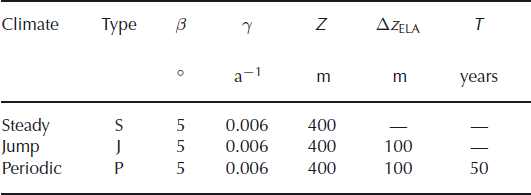
A series of numerical experiments was conducted with varying climate-forcing parameters and different bedrock slopes. To investigate the reaction of the model glacier to climate variations, the equilibrium-line altitude z ELA was changed. As an example, we consider the model experiment with the designation [P/5/0.006/400/100/50] and the corresponding steady state [S/5/0.006/400]. Table 2 defines the model parameters where Δz ELA and T characterize climate oscillations (Equation (50) below), Z = z 0 − z ELA and z 0 is arbitrarily set to 2000 m.
Table 2. Parameters used for designation of FS-model runs
All model runs start from a steady-state geometry which was obtained by letting the glacier evolve for 500 model years at constant z ELA until changes in geometry become negligible (e.g. model run [S/5/0.006/400]). Starting from the steady-state geometry, the glacier is forced by sinusoidally varying the equilibrium line with period T during nT periods, according to the history

Figure 3 shows the climate forcing and the resulting changes in glacier length and volume for nT = 30 (which was mostly used). The reaction of the glacier is initially dominated by large transients that die out after several climate cycles, when the glacier reaction settles into a periodic succession of values with the same period as the external forcing. Four distinct stages of glacier evolution are indicated in Figure 3: the initial and final steady states (SS), the initial transients (IT) after the beginning of periodic forcing, the periodic response (PR) under periodic forcing of the ELA and the final transients (FT) after periodic forcing has been switched off. The response is similar (with opposite sign) for the cases of initially rising or falling ELA. The different stages are investigated in this section.

Fig. 3. (a) The model glaciers are forced with sinusoidal variations of the ELA with 100 m amplitude for 30 climate cycles of length T = 50 years. Solid curves indicate initially rising ELA, and dotted curves initially falling ELA. The response of (b) glacier length and (c) volume (curve styles correspond to the forcing) are shown. Model runs [P/5/0.006/400/±100/50].
A useful way to display the glacier response is the phase space diagram. Figure 4 shows the deviations of glacier length and ice volume from the steady state during the history of Figure 3a. After initial transients (IT, spiralling loops on the left) the response becomes periodic (PR, limit cycle). During the final transients (FT) after the climate becomes constant, the glacier advances considerably at an almost constant volume.

Fig. 4. Phase space diagram showing relative deviations from the steady state (solid dot) during the climate history of Figure 3a. The solid curve represents the response to an initially rising ELA [P/5/0.006/400/100/50] and the dotted line represents the steady states for [S/5/0.006/300…500].
5.1. Steady states
Modelled steady-state glacier geometries are shown in Figure 5. The ice thickness in the upper part of the glacier varies only moderately for different ELAs (different values of Z). The mass flux is maximum at the equilibrium line (indicated with symbols). Due to the varying surface slope, the location of the maximum ice thickness is above the equilibrium line and the maximum flow velocity is below.

Fig. 5. Surface geometries for different ELAs between Z = 100 and Z = 600 m (indicated below the glacier terminus) (runs [S/5/0.006/100 … 600]). Solid dots indicate the horizontal location of the equilibrium line, upward-pointing triangles the maximum ice thickness and downward-pointing triangles maximum flow velocities.
Modelled steady-state glacier geometries for different accumulation rates are plotted in Figure 6. Glaciers are thicker under high mass-balance gradients. Their increased length is mainly due to the mass-balance–elevation feedback, which shifts the horizontal location of the equilibrium line downstream. An eightfold increase of mass-balance gradient (from γ = 0.006 to 0.048 a−1) has only a moderate effect on glacier length and barely doubles glacier volume (Table 3).
Table 3. Results from steady states of the FS-model are shown in columns 2–4. Columns 9–11 show the relative deviations from the FS-model thickness H and volume V of δHG = (HG − H)/H, δHL = (HL − H)/H and δVL = (VL − V)/V calculated with the scaling relations Equations (19), (20) and (21) using r = 0.53 and f = 0.88


Fig. 6. Surface geometries for different mass-balance gradients (runs [S/5/0.006 . . . 0.048/400] indicated below the glacier terminus).The dashed curve shows the glacier geometry of [S/5/0.006/500] for comparison. Solid dots indicate the horizontal location of the equilibrium line, upward-pointing triangles the maximum ice thickness and downward-pointing triangles maximum flow velocities.
The relation between glacier length and volume is shown in Figure 7 for mass-balance gradients γ = 0.006–0.048 a−1 and Z = 100–600 m at bed inclinations of 5° and 10°.

Fig. 7. Volume vs length for steady states at different accumulation rates (runs [S/5/0.006…0.048/100…600]) and for run [S/10/0.006…0.012/100…600] (symbols and dotted lines). Numbers at the right indicate bedrock inclination (5° and 10°) and mass-balance gradient γ; numbers on top represent the elevation difference Z = z
0 − z
ELA. Solid lines show the volumes corrected by ![]() .
.
The steady-state volume can be related to glacier length with a power-law relation V = aLμ . The best fit for various values of γ and Z is μ ∼ 1.39–1.40, as shown in Table 3. Ice thicknesses calculated with Equations (19) and (20) and glacier volumes from Equation (21) agree with the FS-model results (Table 3) within a few percent.
The scaled shapes of steady-state glaciers in a wide range of values for γ and Z is compared in Figure 8. Larger glaciers are somewhat thinner in the accumulation area in a relative sense, and somewhat thicker in the ablation area than small glaciers. This influences the values of ![]() and
and ![]() , but not f (Table 3).
, but not f (Table 3).

Fig. 8. Scaled shapes of steady-state glaciers for Z = 600 m (solid curves) and Z = 200 m (dotted curves) and for mass-balance gradients between 0.006 (uppermost curves) and 0.06 a−1 (lowermost curves). Dots indicate the location of the equilibrium line (β = 5°).
The variation of ice-flow velocity at the surface is shown in Figure 9. The velocity maximum is reached downstream of the half-length of the glacier, with a value within 5% of the velocity calculated with the shallow-ice approximation for the ice thickness H (at the equilibrium line) and the bedrock slope m b:

Fig. 9. Flow velocities for ELAs z ELA between 1900 and 1400 m (Z = 100–600 m indicated). Dotted curves indicate a quadratic function (Equation (52)) for comparison [S/5/0.006/*].
The velocity variation is well approximated by a quadratic function (Reference NyeNye’s (1965) ‘special model’, as indicated in the figure):
where L ∗ = (1 + δ)L corresponds to Nye’s L and δ = 0.07.
5.2. Periodic response
After any initial transients have died out, the glacier response becomes periodic. The glacier geometry, and all associated quantities such as flow velocity, undergo a periodic succession of states f(t) = f(t + T), where T is the forcing period. In a phase space diagram such as Figure 4, the periodic response appears as a closed loop.
Figure 10a shows a phase space diagram of the reaction of a glacier to a forcing with period T between 10 and 1000 years. The volume varies during rapid oscillations, while the glacier length is almost constant (vertical bar in the centre of Fig. 10a). For long oscillation periods, the relative variations in volume and length become nearly equal (20–25%). The long axis of the limit cycle approaches the slope of the steady-state volume–length relation (dotted line in Fig. 10a) with the slope μ from the scaling relation Equation (21). (The same slope is apparent at the low-frequency end of the solid curve in Figure 10b with value arctan μ ∼ arctan 1.41 = 55°.)

Fig. 10. (a) Phase space limit cycles for the periodic response at different forcing periods T = 10–1000 years [P/5/0.006/400/100/T]. Model states follow the cycles in a clockwise direction, starting at the locations indicated with dots. The innermost limit cycle corresponds to a forcing period of 10 years; the outermost to 1000 years. The dotted line indicates the steady states for [S/5/0.006/300…500]. (b) Ellipses were fitted to the limit cycles for different oscillation frequencies. The ellipse orientation (solid) and lengths of the long (dashed) and the short (dotted) axis are plotted. The oscillation period in years is indicated on the top horizontal axis.
The reaction of the glacier lags behind the external forcing. Figure 11 depicts the phase lag and the oscillation amplitude of length, volume and mean ice thickness as a function of oscillation frequency. For very slow climate oscillations, the glacier can adapt to the forcing and the phase lags are small. The amplitude amounts to the differences between the steady-state glaciers at the corresponding ELAs. The phase lag increases with increasing oscillation frequency while the corresponding oscillation amplitudes decrease. At ELA oscillation periods shorter than the volume timescale, glacier volume lags by roughly 90° and glacier length is out of phase (>180°, Fig. 12). These results agree qualitatively with the responses obtained by Reference NyeNye (1965) and Reference HutterHutter (1983) for their ‘special model’.

Fig. 11. (a) Relative oscillation amplitude and (b) phase lag of volume (solid), length (dash-dotted) and mean thickness (dashed) as a function of frequency [P/5/0.006/400/100/*]. The oscillation period in years is indicated on the top horizontal axis.
Figure 12 shows that the ice thickness (and with it, the flow velocity) has a delayed reaction to a change in climate along the whole glacier. The amplitude and the phase lag increase along the glacier flowline and markedly increase towards the snout, which may be a feature of the no-slip basal boundary condition adopted here. Both amplitude and phase lag depend on the forcing frequency in a manner similar to the change in mean thickness in Figure 11. In practice, this has the consequence that observed changes of glacier surface elevation are not indicators of present climate, but are a delayed reaction to past climate variations.

Fig. 12. (a) Oscillation amplitude and (b) phase shift along the glacier of ice thickness (solid curve) and flow velocity (dashed curve) [P/5/0.006/400/100/50].
5.3. Transient response
During the transitions from steady state to periodic oscillations and back, the model glaciers experience large transient oscillations (Fig. 3). The size and number of initial transient oscillations depend strongly on the forcing period. Figure 13 shows that, for short forcing periods (compared to τ v), the trajectory in phase space wanders far away from the limit cycle of the periodic oscillation and arrives there only after several loops. In contrast, for long forcing periods (compared to τ v) the transient trajectory is always close to the limit cycle. Figure 14a shows that the amplitudes of the initial and final transient oscillations increase with forcing period. Since the size of the limit cycle increases, the relative size of the transients decreases. From Figure 14b it is clear that both the initial and final transients mainly affect glacier length for forcing periods that are shorter than τ v, whereas variations are approximately constant. The phase space diagrams (Figs 4 and 13) illustrate this nicely.

Fig. 13. Phase space diagrams showing relative deviations from the steady state (solid dot) during forcing at periods of T = 20, 50, 90, 120 years [P/5/0.006/400/100/T]. The volume timescale is τ v = 79 years. The dotted line indicates the steady states for [S/5/0.006/300… 500].

Fig. 14. (a) Relative sizes of the initial and final transients for different forcing frequencies ω for model runs [P/5/0.006/400/100/10… 1000]. The volume timescale is τ v = 79 years. (b) Size of initial and final transients with respect to the size of the limiting cycle. Shown are initial transient length (solid) and volume (dash-dotted) and final transient length (dashed) and volume (dotted). The oscillation period in years is indicated on the top horizontal axis.
6. Discussion
6.1. Scaling relations
Scaling relations of the form V = aLμ relating glacier volume to length have been derived in Equations (16) and (21). Even if our assumptions about glacier geometry are different from those exploited by Reference Bahr, Meier and PeckhamBahr and others (1997), the exponents μ = 1.25 and 1.4 are almost the same. In our approximation, the glaciers are infinitely wide such that no valley shapes are taken into account. Our mass balance varies with elevation and therefore only implicitly over the distance along the glacier. That these very different approaches yield similar results can be taken as a confirmation of the universality of such scaling relations.
A major improvement over previous approaches is that the dependence of a on mass-balance gradient and mean bed and surface slope is made explicit and is of the form
for flat-bed and inclined glaciers, respectively. Even if our assumptions about geometry are simplistic, we still suspect that Equation (53) should be applicable for more realistic geometries. Figure 7 shows that correction of the FS-model volumes leads to a very close clustering of values along a line (solid lines). It is likely that empirical data, corrected for mean bed slope and mean mass-balance gradient, would show a similar improvement. Resulting volume–area plots would then show a smaller spread of the data from which better scaling parameters could be deduced.
6.2. Volume timescale
Equation (29) shows a decrease of τ v with increasing ζ (and therefore L, Equation (38)). This is the essence of Equation (25): as glacier length increases, the terminus moves to a lower elevation and the net balance at the terminus becomes increasingly negative. This is partially compensated by the simultaneous increase in ice thickness H to provide enough mass flux from the accumulation area to the ablation area. Our result agrees qualitatively with Reference Bahr, Pfeffer, Sassolas and MeierBahr and others (1998) but with a different functional relation between τ v and ζ.
In nature, small glaciers are usually steeper and thinner than long glaciers. The strong dependence of ζ on m
b in Equation (38) shows that long glaciers have long reaction times not because of their size, but because of their relative flatness compared to short glaciers. The geometric quantity ![]() in Equation (38) can be written in terms of total bedrock elevation difference Δz
b = m
b
L as
in Equation (38) can be written in terms of total bedrock elevation difference Δz
b = m
b
L as ![]() Thus ζ increases (τ
v decreases) as the elevation difference Δz
b increases for constant glacier length. Conversely, longer glaciers have smaller ζ and therefore longer reaction times for constant total elevation difference Δz
b.
Thus ζ increases (τ
v decreases) as the elevation difference Δz
b increases for constant glacier length. Conversely, longer glaciers have smaller ζ and therefore longer reaction times for constant total elevation difference Δz
b.
As has been pointed out (Reference Harrison, Elsberg, Echelmeyer and KrimmelHarrison and others, 2001), the volume timescale not only determines how long it takes to reach a new steady state after a step change in climate (according to Equation (1)), but is also a scale for the ultimate volume change ΔV ∞ = B′τ v, where B′ is the change in net balance integrated over the initial geometry. This assumption works very well for the volume timescale calculated with Equation (29), even for large changes in ELA. An example of the reaction of the FS-model glacier [S/5/0.006/400] to a step change in ELA of ±100 m is shown in Figure 15.

Fig. 15. Reaction of the FS-model glacier [S/5/0.006/400] to a step disturbance in climate. (a) The ELA is shifted by ±100 m. (b) Solid curves show the reaction of glacier volume [J/5/0.006/400/±100]. Dashed lines show the reaction of the dynamical system (Equation (40)) for Ta calculated with ![]() and dotted curves for f
⋆ = 1. (c) The length change, as for (b). The grey bar marks the arrival of a kinematic wave.
and dotted curves for f
⋆ = 1. (c) The length change, as for (b). The grey bar marks the arrival of a kinematic wave.
Glacier volume starts changing immediately due to balance changes everywhere. In contrast, the length change is only substantial after a certain delay which is due to glacier dynamics. For an advancing glacier, the explanation is that ice thickness close to the terminus has to increase to provide higher mass flux to the terminus, which is nicely described by the theory of kinematic waves (e.g. Reference NyeNye, 1960; Reference HutterHutter, 1983). Indeed, a kinematic wave starting at the equilibrium line and moving with a four- to five-fold surface velocity would arrive at the terminus after 19 years (marked with a bar in Fig. 15).
6.3. Minimum glacier size
Equation (29) predicts that glaciers with the same value of ζ, and therefore (Equation (38)) the same value of
have the same volume timescale. Decreasing the steady-state glacier length for given m b and γ eventually leads to a critical length L crit corresponding to ζ crit = 1 (from Equation (29)) for which the volume timescale becomes infinite. For glaciers that are shorter than L crit, the volume timescale is negative and steady-state configurations are not stable. Upon a slight change of ELA, the total mass balance B′ is either positive or negative and the glacier volume either grows or decays exponentially (as described by Equation (1)). As a consequence, no steady-state glaciers that are shorter than L crit can exist. Figure 16 shows the minimum stable glacier lengths on inclined bedrock for different mass-balance gradients.

Fig. 16. Minimum stable steady-state glacier lengths plotted against bedrock slope m b for different mass-balance gradients γ (indicated next to curve).
6.4. Transient response
The response of simple model glaciers to periodic changes in ELA has some interesting aspects. During the transition from a steady-state to a periodically varying climate, glacier volume and length show large transients for forcing periods that are shorter than the volume timescale (marked IT in Figs 3 and 4). These transients eventually fade after several climate cycles.
The large initial transients are caused by the rapid initial depletion (or overfilling) of the ice reservoir in the accumulation area, and are not an effect of the mass-balance–elevation feedback. FS-model runs with a position-dependent mass-balance distribution, and with a comparable variation of the equilibrium line, qualitatively give the same results as obtained with the elevation-dependent mass balance (Equation (3)). The evolution of ice thickness and velocity under the climate scenario of Figure 17a is shown in Figure 18. The initial rapid thinning in the accumulation area (Fig. 18a) leads to lower flow velocities and therefore to slower mass transport (Fig. 18b), which in turn is responsible for the increasingly rapid volume loss in the ablation area. After the perturbation, ice thickness slowly recovers to the initial state.

Fig. 17. Reaction of the FS-model glacier [S/5/0.006/400] to a short disturbance in climate. (a) The ELA is sinusoidally varied for 25 years. (b) Solid curves show the reaction of glacier volume to short disturbances and periodic forcing [P/5/0.006/400/100/50]. Dashed curves show the reaction of the dynamical system (Equation (41)) for τ
a calculated with ![]() and dotted lines for f
⋆ = 1. (c) The length change as for (b).
and dotted lines for f
⋆ = 1. (c) The length change as for (b).

Fig. 18. Transient response of the FS-model glacier [S/5/0.006/400] to a short sinusoidal disturbance in climate for 25 years (Fig. 17a). Changes of (a) ice thickness and (b) flow velocity along the glacier are shown every 10 years for the first 40 years (solid curves). Dashed curve: 50 years; dotted curvevs: 100, 200 and 300 years.
The final transient (marked FT in Figs 3 and 4) occurs during the transition from an oscillating climate to a steady state. During this phase, volume remains nearly constant but glacier length shows a pulse which is due to a kinematic wave originating from the under- or overfull reservoir area.
6.5. Dynamical system
How well the dynamics of the FS-model glaciers can be reproduced with the dynamical system Equation (40) or the linearized version Equation (41) (corresponding to the harmonic oscillator Equation (46)) can be assessed by comparing the evolution for different forcing scenarios. The assumption of a relaxation-type length response (Equation (30)) is ad hoc, and therefore a mismatch will most likely be visible in the length change.
The dynamical system solution in Figure 15 for a step change in climate follows the FS-model results closely, especially for the volume change. Results for both dynamical systems (Equations (40) and (41)) are almost indistinguishable. In the dynamical system, the length change sets in immediately whereas it is delayed in the FS-model.
To test the response to periodic forcing, the steady-state FS-model glacier [S/5/0.006/400] is forced with short (nT = 0.5) and long (nT = 30) periodic ELA variations (Equation (50; Figs 17a and 3a). Figure 17b shows that the volume is closely reproduced by the dynamical system with τ v = 79 years and τ a = 15 years calculated from Equations (29) and (37). The corresponding ω 0 = 0.029 and λ = 0.030 indicate that this corresponds to a slightly overdamped harmonic oscillator.
While the dynamical system satisfactorily reproduces the modelled volume change, the phase of the length changes differs greatly from the FS-model result. This indicates that a relaxation-type evolution of glacier length is not useful to predict the evolution of glacier length at forcing periods shorter than the volume timescale, and should be replaced by a better parameterization of glacier terminus dynamics. Such an improved parameterization would likely contain an inertia term producing a delay in reaction.
The exact value of the parameter f
⋆ in the length evolution equation seems not to be crucial, as ![]() and f
⋆ = 1 give similar results (Figs 15 and 17). It therefore seems reasonable to adopt
and f
⋆ = 1 give similar results (Figs 15 and 17). It therefore seems reasonable to adopt ![]() or f
⋆ = f, the latter of which would lead to simplified Equation (37) for τ
a.
or f
⋆ = f, the latter of which would lead to simplified Equation (37) for τ
a.
6.6. Critically damped harmonic oscillator
From South Cascade Glacier (Washinton, USA) data, Reference Harrison, Raymond, Echelmeyer and KrimmelHarrison and others (2003) assumed that the glacier response can be described with a critically damped harmonic oscillator (λ = ω 0). Indeed, using values for South Cascade Glacier (γ = 0.024 a−1, m b = 0.14, L = 3 km, H e = 123 m ⇒ H ∼ 100 m and Z = 190 m) gives ζ ∼ 1.87, ω 0 = 0.0517 and λ = 0.0522 which is close to critical damping. With the above selection of values, we also obtain τ v = 48 years and τ a = 7.8 years, in agreement with the values given by Reference Harrison, Raymond, Echelmeyer and KrimmelHarrison and others (2003).
7. Conclusions
A novel low-order model of a simple glacier (called the LV-model) was developed, consisting of two volumes joined at the equilibrium line by a flux element. Exact and approximate analytical expressions were derived, which include
-
1. a dynamical system (Equation (40)) in the variables L and V that describes glacier evolution under variations of the equilibrium line;
-
2. volume–length scaling relations (Equations (17) and (21)) of the form V = aLμ , with μ = 1.25 and a
 for a flat base (m
b = 0), and μ = 1.4 and a
for a mountain glacier geometry (m
b > 0);
for a flat base (m
b = 0), and μ = 1.4 and a
for a mountain glacier geometry (m
b > 0); -
3. a correction factor that can be used to improve empirical volume–area scaling relations by taking mass-balance gradient γ and mean bedrock slope m b into account;
-
4. explicit values for the volume and area timescales as a function of a parameter ζ, the elevation difference of the ablation area scaled by the effective ice thickness; and
-
5. a minimum size for stable glaciers, depending on mass-balance gradient and bedrock slope.
For comparison and further experiments, a transient, full-Stokes FE flow model for arbitrary flowline bedrock geometries (FS-model) was developed. Results from this model on constant bedrock slopes under transient variations of the ELA show that
-
1. the transient response of glacier volume to periodic forcing is delayed by one-quarter of the forcing period for periods smaller than τ v;
-
2. the transient response of glacier length to periodic forcing is delayed by one-half of the forcing period for periods smaller than τ v;
-
3. glacier length and volume show large initial and final transient responses to periodic forcing, which render the climatic interpretation of such records difficult; and
-
4. surface elevation and velocity changes along a glacier show an important time lag to climate forcing (careful evaluation is therefore needed when interpreting surface elevation changes as a climate signal).
Comparison of results of the LV-model and the FS-model under the same climate variations shows that simple, low-order or macroscopic glacier models give very good results for the transient evolution of glacier volume. For the prediction of glacier length changes on timescales shorter than τ v, the commonly assumed relaxation-type relation for glacier length (Equation (30)) should be replaced by a more realistic parameterization including a delay term. The description of a glacier as a critically damped harmonic oscillator captures the essential dynamics for the investigated simple geometries.
Acknowledgements
This work greatly profited from discussions and thoughtful comments on earlier versions by W. Harrison, M. Funk, M. Truffer and K. Hutter. Valuable reviews by C. Raymond and T. Jóhannesson and by the scientific editor R. Greve are gratefully acknowledged. This research was financed by Swiss National Science Foundation grant No. 200021-113503/1 and US National Science Foundation grant No. OPP-0327067.


