


Introduction
Satellite passive microwave data indicate an accelerated decline in the Arctic sea-ice extent over the last decade (Reference StroeveStroeve and others, 2008), and a record minimum ice extent was observed in September 2007 (Reference Maslanik, Fowler, Drobot and ZwallyMaslanik and others, 2007). Submarine measurements of ice draft have hinted at a similar demise in the thickness of the ice pack (e.g. Reference Rothrock, Yu and MaykutRothrock and others, 1999); new laser and radar altimetry measurements from satellites such as Envisat and the Ice, Cloud and land Elevation Satellite (ICESat) are now providing the further detail needed to resolve sea-ice volume on basin scales (e.g. Reference Kwok, Cunningham, Wensnahan, Zwally and YiKwok and others, 2009). the latest satellite altimetry observations of sea-ice freeboard (height of sea-ice floe above local sea level) indicate a decline in sea-ice thickness and volume over the last 5 years (e.g. Reference Giles, Laxon and RidoutGiles and others, 2008; Reference Farrell, Laxon, McAdoo, Yi and ZwallyFarrell and others, 2009; Reference Kwok, Cunningham, Wensnahan, Zwally and YiKwok and others, 2009). These observations show a particular thinning over the perennial ice regions (e.g. Reference Farrell, Laxon, McAdoo, Yi and ZwallyFarrell and others, 2009), which is consistent with the observed loss of the oldest, multi-year ice-pack (Reference Maslanik, Fowler, Drobot and ZwallyMaslanik and others, 2007; Reference Nghiem, Rigor, Perovich, Weatherly and NeumannNghiem and others, 2007; Reference Comiso, Parkinson, Gersten and StockComiso and others, 2008). Continued monitoring of Arctic-wide sea-ice thickness and volume change during the coming decade using satellite altimetry is necessary to determine whether these recent observations are part of a sustained negative trend in Arctic ice thickness or a reflection of the natural, interannual variability. Continued loss of Arctic sea ice will have major environmental and societal implications (e.g. see ACIA, 2005).
To meet such requirements, the European Space Agency (ESA) launched the CryoSat-2 satellite radar altimeter system on 8 April 2010, and the US National Research Council decadal survey has recommended a follow-on mission to ICESat (NRC, 2007). the primary goal of ICESat-2 is to measure changes in the Earth’s ice sheets and sea ice with an accuracy and precision that allows for elevation change detection. the satellite, which NASA plans to launch in late 2015, will also measure vegetation canopy height for large-scale vegetation biomass estimates (Reference AbdalatiAbdalati and others, 2010). the Advanced Topographic Laser Altimeter System (ATLAS) instrument on board ICESat-2 is designed to obtain precise laser altimetric measurements of surface elevation over the Earth’s cryosphere, specifically the Greenland and Antarctic ice sheets, and Arctic and Southern Ocean sea ice. ICESat-2 builds on the technological achievements demonstrated by its predecessor ICESat, whilst offering considerable improvements over ICESat in that it will provide year-round measurements of sea-ice surface elevation. the design of the ATLAS instrument is currently in the planning stages and may differ considerably from the Geoscience Laser Altimeter System (GLAS) on board ICESat. A digital laser altimetry approach has been proposed which would consist of a high-pulse-repetition laser with overlapping ~10m footprints, dense along-track sampling, and energy output split into nine beams. Laser output energy will be selected so that the photon-counting detector will detect one photon for each overlapping footprint with a probability of ~80% (Reference AbdalatiAbdalati and others, 2010).
To maintain continuity between the end of the ICESat mission, in late 2009, and the launch of ICESat-2, NASA has established the IceBridge mission (see http://www.espo.nasa.gov/oib/). IceBridge comprises a series of airborne surveys of the cryosphere, in areas of critical importance including the Arctic and Southern Ocean sea ice, to be conducted over the next 6 years. Laser and radar altimetric mapping of sea-ice elevation and snow thickness will be used to derive the sea-ice freeboard and thickness of the winter-time ice pack in both hemispheres. IceBridge aircraft typically carry two laser altimeters, the Airborne Topographic Mapper (ATM; Reference KrabillKrabill and others, 2002) and the Land, Vegetation and Ice Sensor (LVIS; Reference Hofton, Blair, Luthcke and RabineHofton and others, 2008).
These systems operate at different flight altitudes and offer a range of spatial coverage of the ice pack from the 100mscale (ATM) to the km scale (LVIS) in the across-track direction.
While all four instruments (ICESat/GLAS, ICESat-2/ATLAS, LVIS and ATM) use a common measurement approach in laser altimetry, each system obtains a unique geospatial sampling of the ice pack, such that the resolution of the sea-ice freeboard measurement is different in each case (Table 1). A major aim of the IceBridge mission is to provide a continuous sea-ice thickness time series over the next 6 years, thereby ‘bridging the gap’ between ICESat and ICESat-2. Therefore data from all four sensors will necessarily be combined and compared. To address the issue of combining measurements with varying resolutions and investigate its potential impact on estimates of sea-ice freeboard, we compare the sampling methods utilized by the conventional analogue systems of ICESat, LVIS and the ATM, with the multi-beam, digital photon-counting system proposed for ICESat-2. We construct two sea-ice models, which represent typical first-year and multi-year sea-ice regimes. We assess the ability of each laser system to reproduce the mean freeboard, lead and ridge height of the reference sea-ice model and we discuss potential biases in lead detection and sea surface elevation. Given the multi-beam, photon-counting approach proposed for ICESat-2, we consider the use of along-track sampling for unambiguous identification of leads within the ice pack. Accurate identification of leads is critical for precise estimation of sea-ice freeboard and hence ice thickness (Reference Farrell, Laxon, McAdoo, Yi and ZwallyFarrell and others, 2009).
Table 1. Specifications for current satellite and airborne laser altimetry systems compared with those proposed for the ICESat-2 system. Estimated precision (1σ) is based on system performance over ice sheets, with the exception of GLAS where precision refers to performance over sea ice

Current and Planned Laser Altimetry Systems
Table 1 summarizes the specifications for the four satellite and airborne laser altimeters considered in this study, indicating the measurement resolution of each system. To aid the reader’s visualization of differences between each laser instrument, a depiction of footprint configurations, including footprint diameter, along-track and across-track spacing, is illustrated in Figure 1a. As indicated in Table 1, both the LVIS and ICESat-2 systems comprise ground-track coverage that extends beyond the 100m across-track segment, shown in Figure 1a.

Fig. 1. (a) Schematic diagram of footprint configuration (diameter, along-track and across-track spacing) for each laser altimeter system (ICESat/GLAS, LVIS, ATM and proposed ICESat-2/ATLAS system) across a 100m wide swath. Note the full LVIS swath extends to ~2 km and is thus beyond the 100m across-track segment depicted here. Furthermore only the central beam-triplet of the ICESat-2 system is depicted here (two more beam triplets would align ~3 km either side of the central segment). (b) Proposed nine-beam configuration for the ICESat-2 system with high-,medium- and low-energy beam distribution and (c) ICESat-2 beam alignment given a satellite yaw of ~2˚.
The GLAS instrument on ICESat consisted of a single-beam laser altimeter with a 50–70m footprint diameter, spaced every 172 m along-track. the state-of-the-art laser-ranging capabilities of ICESat, and post-processing of reflected laser pulses (waveforms), provides data that are precise to ~2 cm over sea ice (e.g. Reference Kwok, Zwally and YiKwok and others, 2004), and useful for profiling the complex sea-ice environment. LVIS is an airborne laser system, similar to GLAS, that operates at altitudes of about 10 km. Depending on flight altitude, the LVIS scanning laser altimeter obtains footprints 10–25m in diameter, across swath widths of about 2 km (80 footprints), with contiguous footprints in both the across-and along-track directions (Reference Hofton, Blair, Luthcke and RabineHofton and others, 2008). This has advantages for cryospheric investigations since the system provides highly detailed mapping of ice elevation and surface characteristics. Both the ICESat/GLAS and LVIS instruments operate at near-infrared wavelengths (1064 nm).
*From Reference KrabillKrabill and others (2002). †From Reference Hofton, Blair, Luthcke and RabineHofton and others (2008). ‡From Reference Kwok, Zwally and YiKwok and others (2004). ¶From Reference AbdalatiAbdalati and others (2010).
The ATM airborne laser altimeter operates at a wavelength of 532 nm with a pulse repetition frequency of 5 kHz and a scan angle of ~15˚. Depending on flight altitude, swath width can range from 100 to 400 m, while footprint size is ~1m. Footprint separation at the center of the swath is typically ~5m in the along-track direction. the ATM instrument has historically been used for elevation change detection of the Greenland ice sheet (Reference KrabillKrabill and others, 2002; Reference Thomas, Frederick, Manizade and MartinThomas and others, 2009), but data have also been collected over sea ice (e.g. Reference Connor, Laxon, Ridout, Krabill and McAdooConnor and others, 2009).
Figure 1b shows one of the proposed beam configurations for the ICESat-2 system. In this example, the configuration includes a nine-beam approach with a distribution of high-,medium- and low-energy beams. the approach of variable pulse energy is taken so as to obtain unsaturated return pulses across surfaces with a range of albedos, particularly ice-sheet margins, glacier calving fronts and sea ice. the 3×3 square of spots will be rotated by ~2˚ relative to the satellite velocity vector such that the beams will be offset in the across-track direction. Here the three parallel beam triplets align ~3 km apart in the across-track direction, to produce a high-energy central three-beam track, and two lower-energy side beams, also with three beams each (Fig. 1c). A photon-counting approach is utilized where single photons are detected from within 10m diameter footprints (see fig. 12 in Reference AbdalatiAbdalati and others, 2010). Uncertainty in the exact geolocation of photons within the footprint gives rise to a vertical range precision of ~10 cm. A frequency doubler on the laser is used so that efficient photon-counting detectors, which are sensitive to green wavelengths (532 nm), may be used (Reference AbdalatiAbdalati and others, 2010). the probability of detecting one photon per footprint depends on many factors, including surface albedo as well as pulse energy. Here we assume the laser operates at a 15 kHz pulse-repetition frequency, such that footprints are oversampled and overlap every 50 cm along-track. Along-track averaging of a number of pulses will be used to improve measurement accuracy. One advantage of the system will be flexibility in the length scale chosen for such along-track averaging depending on surface conditions (ice sheet, sea ice, vegetation, etc.). the ideal along-track averaging length scale required over sea ice to obtain accurate lead elevations, uncontaminated by freeboard from nearby ice floes, is a key and ongoing investigation of the ICESat-2 science definition team. an assessment of lead width in the Arctic can be used to determine the ideal length scale, which may be as short as ~15 m.
Model Set-Up
We construct a reference sea-ice freeboard dataset in order to compare the various sampling strategies employed by the four laser altimeter systems. To do this we create a high-resolution grid with 50cm×50cm gridcells, placed in a 100m wide by 25 km long model domain. an along-track distance of 25 km is chosen for the model, since this represents the typical length scale along which sea-ice freeboards are averaged for regional and basin-scale studies using actual satellite or airborne data. Initially we use a set of ATM elevation measurements gathered over Arctic sea ice to seed the model grid with a realistic distribution of sea-ice surface elevation and surface roughness. (The ATM data used here were collected in March 2006 during a NASA aircraft survey of sea ice in the Beaufort and Chukchi Seas (Reference Cavalieri and MarkusCavalieri and Markus, 2006), conducted as part of an Aqua Advanced Microwave Scanning Radiometer for Earth Observing System (AMSR-E) instrument validation campaign.) Since the resolution of the ATM data is lower than that of the model, we use the continuous curvature surface gridding algorithm from the Generic Mapping Tools (GMT) software package (Reference Wessel and SmithWessel and Smith, 1998), applying a tension factor of 0.3, to interpolate across gridcells containing no ATM data points. We define local sea level as 0m and set a number of gridcells to sea level, which effectively defines the number and location of leads within the model domain. Sea-ice elevation is referenced to this level, and freeboard is thus defined for all elevations above sea level. Here we define freeboard as the height of the sea ice and snow above local sea level since laser altimeters measure this elevation (Reference Farrell, Laxon, McAdoo, Yi and ZwallyFarrell and others, 2009). In addition to classifying surface elevation and roughness, we prescribe reflectivity, based on the albedo of different sea-ice types at visible wavelengths, as documented by Reference Perovich and rantaPerovich (1998). Leads are prescribed a reflectivity of 0.2, while the reflectivity of sea-ice floes ranges from 0.6 to 0.85, depending on sea-ice freeboard. This step allows for a reasonable calculation of the probability of detecting a return photon over sea ice with a variable surface albedo, in the case of the ICESat-2 photon-counting simulation.
To compare the performance of the laser sensors over realistic sea-ice environments, we construct two sea-ice models: the first represents a first-year sea-ice pack with a high lead fraction; all sea-ice elevations above 0.45 m are defined as sea-ice floes, while any sea ice between 0 and 0.45m is reset to sea level and redefined as a lead. the second model represents a typical multi-year ice pack with a high proportion of thick, ridged sea-ice floes and a lower percentage of leads. All sea-ice floes have freeboard ≥1m, and any data between 0 and 1m are redefined as sea level and prescribed an elevation of 0 m. the resulting step function in freeboard between sea level (elevation = 0 m) and sea-ice floes (elevation ≥0.45m or 1 m, depending on model) allows for easier analysis of the effect of mixed returns, i.e. the contamination of sea surface elevation through inclusion of elevations from nearby sea-ice floes, at lead–floe boundaries.
Since the objective of this study is to compare measurement biases introduced by the spatial sampling of each laser system, we do not treat range delays due to instrument bias, orbit error, atmospheric attenuation or forward scattering. the green wavelength (532 nm) proposed for ICESat-2 will result in penetration of some laser energy into open-water leads. Here we assume that subsurface returns will be filtered to mitigate the impact of laser pulse penetration into open water. Additionally a near-infrared beam used in conjunction with the green channel may be employed to further resolve ambiguities (Reference AbdalatiAbdalati and others, 2010). the ICESat-2 photon-counting simulation presented here assumes that an algorithmic approach for separating ground returns from solar background noise will be utilized for analysis of actual ICESat-2 data. Therefore the effect of solar background photons is not included in this ICESat-2 simulation.
Our analysis has been conducted under the assumption of clear atmospheric conditions with no data loss through cloud obstruction. While airborne campaigns are generally conducted in cloud-free conditions, this is impossible with satellite missions. Analysis of ICESat data suggests that clouds can impact the accuracy of the elevation retrieval (Reference Fricker, Borsa, Carabajal, Quinn and BillsFricker and others, 2005), and in some cases up to 37% of the data were discarded over sea ice (Reference Farrell, Laxon, McAdoo, Yi and ZwallyFarrell and others, 2009). We therefore expect some data loss when analyzing actual ICESat-2 data, but the implications of this are not included in this study.
Results and Discussion
A 2 km segment of the first model, which depicts a thin sea-ice pack with many leads, is shown in Figure 2a, while Figure 3a shows a segment of the second model which describes a thick, ridged sea-ice pack containing a few narrow leads. Based on the footprint specifications outlined in Table 1, the model surfaces are subsequently sampled using the four measurement patterns. We calculate sea-ice freeboard for each laser altimetry scenario and compare these results with the reference data. Examples of the resulting sampling patterns (reflecting footprint size and spacing) across the ice surface, and the derived freeboards, are illustrated in Figures 2b and 3b for both models.

Fig. 2. (a) 2 km segment of modeled first-year sea-ice freeboard (m). (b) Sampling pattern and freeboard (m) as simulated for the ICESat system, LVIS, ATM and the proposed ICESat-2 configurations. (c) Comparison of expected freeboard across model domain segment (black curve) with freeboard derived from ICESat (dark red), LVIS (light green), ATM (dark green) and ICESat-2 (grey dots). the raw ICESat-2 data are processed in the along-track direction, using a 15 m boxcar filter (dark blue), and the local sea surface height profile is defined (cyan line).
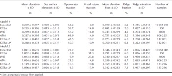
Analysis is conducted using the two 25 km long sea-ice models described earlier, and the results of the individual sampling strategies are compared in Table 2. Derived sea-ice freeboard profiles associated with the 2 km long segments are illustrated in Figures 2c and 3c. the expected sea-ice freeboard (black lines, top panels) may be compared to the freeboard derived for the ICESat (dark red lines), LVIS (light green lines) and ATM (dark green) systems (middle panels). the LVIS and ATM systems accurately reproduce lead elevation, sea-ice freeboard (height above local sea level) and surface variability (or roughness). Slight contamination of the LVIS lead elevation at a lead–floe boundary is observed in model 2 (Fig. 3c) at ~1.5 km along-track, but does not appear to be an issue at other lead–floe transitions. the recorded ICESat freeboards are accurate compared to the expected values, but the along-track sampling at ~172m severely restricts analysis of surface roughness, along-track elevation variability and the ability to resolve leads. This is particularly clear in Figure 3c (model 2) where only one ICESat footprint falls within a lead.

Fig. 3. Same as Figure 2, but for multi-year sea-ice freeboard.
Table 2. Summary of sea-ice freeboard and sea surface elevation, as observed by each laser altimetry system along a 25 km transect, for modeled first-year (model 1) and multi-year (model 2) sea ice. SD: standard deviation
Freeboard measurements yielded by the proposed ICESat-2 photon-counting approach are included in the lower panels of Figures 2c and 3c. Individual measurements of elevation from the three parallel beams (grey dots) produce a data cloud, which represents returns from all overlapping 10m diameter footprints used to sample the model grids. Along-track averaging on a pulse-to-pulse basis (dark blue line) indicates the reduction in noise level that may be expected when a 15 m along-track (boxcar) filter is applied. Flexibility in the along-track averaging length scale will allow for the ideal balance between a reduction in measurement noise and the preservation of surface roughness characteristics and true elevation variability. Furthermore, the individual photon detection of the ICESat-2 system prevents the retrieval of ‘mixed returns’ (i.e. a reflection from the boundary at a lead–floe transition); indeed Figures 2c and 3c illustrate that individual photons are returned from even the narrowest leads. Thus it may be possible to process pulse returns from leads and sea-ice floes separately to obtain more accurate along-track sea surface height profiles. Here we use the first mode of the elevation distribution to indicate lead elevation and define the local sea surface height profile (cyan line, Figs 2c and 3c).
Table 2 summarizes the full set of results obtained after sampling the entire 25 km long model surfaces with each laser sensor and allows for comparison with the expected sea-ice freeboard, water fraction, lead elevation and ridge statistics, as derived directly from the two model datasets. the analysis suggests that the three analogue laser systems (ICESat/GLAS, LVIS and ATM) successfully reproduce mean sea-ice freeboard within 25 km segments to within 1 cm or less (Table 2, column 1). the standard deviation of freeboard is a representation of surface roughness in our simulation study. the ATM system is successful in reproducing the surface roughness statistics defined in the models. This result is expected since ATM data were used to initialize the model elevation distribution and the models therefore describe surface roughness at the scale of the ATM instrument. the larger footprints of the LVIS and ICESat systems result in a slight underestimate of surface roughness since the analogue return pulse acts to average small-scale surface roughness. Results for the photon-counting approach proposed for ICESat-2 suggest mean freeboard biases of ~7–11cm over 25 km segments compared with the reference dataset. the probability of detecting photons reflected from high-albedo surfaces such as ice floes is higher than the probability of detecting photons reflected by dark surface such as leads. the photon-counting simulation used here to illustrate ICESat-2 data will therefore preferentially sample ice floes (rather than leads). This may explain some of the observed elevation bias with respect to the modeled elevation, although further investigation is required. Application of a 15 m along-track smoothing algorithm to the raw data acts to reduce this elevation bias, and results in mean sea-ice freeboards that are within 5 cm of the expected values.
Mean ice-floe elevation is retrieved to within a few centimeters of the expected values by all sensors (Table 2, column 5). the ATM and ICESat-2 sensors produced the most accurate statistics on ridge fraction and height compared with the model data (Table 2, columns 6 and 7). For both ice regimes, the ATM system reproduces ridge height and variability almost exactly, while ICESat-2 resolves ridge fraction, and ridge and ice floe height to cm-level accuracy. Both the LVIS and ICESat sensors underestimate the percentage and height of ridges in the model grids by 10–15cm due to (1) averaging of surface elevation within the 25 or 50 m footprints and (2) the increased potential for obtaining mixed returns at lead–floe boundaries.
The modeled sea-ice surface was constructed such that all leads had an elevation of 0m, and there were no sea-ice floes with elevations between local sea level and a defined elevation threshold (0.45m for model 1; 1 m for model 2). Figure 4 illustrates the freeboard distributions derived for each laser sensor compared with the expected freeboard distribution for the two models. All four laser systems produce anomalous measurements over the elevation range between sea level and the defined ice-floe elevation threshold, suggesting either (1) contamination of lead elevations by nearby sea-ice floes in the case of larger footprints such as those used by ICESat and LVIS (i.e. mixed returns), or (2) measurement noise in the ATM and ICESat-2 cases. Furthermore, the freeboard distributions indicate the underestimation of the open-water fraction by each laser system compared with the models. However, Figure 4 suggests that analysis of the bimodal freeboard distributions, which are reproduced by all sensors, could help define local sea surface elevation, since the first mode is associated with sea level, while the second mode represents sea-ice floe elevation.

Fig. 4. Elevation distribution for modeled (a) first-year (model 1) and (b) multi-year (model 2) sea ice derived for the model data and each laser altimetry system simulation. *15m along-track boxcar filter applied to ICESat-2 data.
Using the lowest mode of the elevation distributions to indicate local sea level, we calculate sea surface elevation (Table 2, column 2). For model 1, which represents a first-year ice pack with a high lead fraction, sea surface elevation bias is low (~1 cm or less), although variability about the mode is at the decimeter level, indicating measurement noise (precision). All systems resolve an open-water fraction that is slightly lower than the model value, and the ICESat, LVIS and ICESat-2 distributions all include a mixed return fraction of 10–14% (Table 2, column 4). In the case of the multi-year ice model (model 2) which has thicker freeboard and fewer, narrow leads, sea surface elevation bias is of order 1 cm to several centimeters, and the variability about the first mode is also higher for the model 2 results. the fraction of open water (Table 2, column 3) is underestimated by the ICESat, LVIS and ICESat-2 systems, and the fraction of mixed returns is also high. the potential exists for mixed returns to bias the estimate of sea surface elevation if these returns are incorrectly flagged as leads. Significant bias in the estimation of local sea surface elevation would impact the derived sea-ice freeboard and hence ice thickness. Along-track filtering or other post-processing could potentially reduce the impact of mixed returns.
Conclusions
Continuous sea-ice monitoring over basin scales is becoming increasingly important in light of recent satellite observations showing the loss of the areal extent, thickness and volume of the Arctic sea-ice pack. NASA plans the launch of ICESat-2 in late 2015 to continue the time series of sea-ice elevation measurements and volume change detection begun with ICESat in 2003. To mitigate the inevitable loss of data due to the gap in satellite coverage between the end of the ICESat mission and the launch of ICESat-2, NASA has initiated Operation IceBridge, a series of airborne surveys that will continue to collect cryospheric data in key areas.
Here we have considered potential difficulties when comparing and combining data from four currently operating or planned laser altimetry sensors (ICESat/GLAS, LVIS, ATM and ICESat-2/ATLAS). Each altimeter yields spatial sampling of the sea-ice pack at different resolutions and along-track scales. We have investigated the impact of such spatial sampling on estimates of sea surface elevation and sea-ice freeboard. We have compared the sampling methods utilized by the conventional analogue systems (ICESat, LVIS and ATM) and the multi-beam, digital system proposed for ICESat-2, with modeled sea-ice elevation distributions. Overall the analogue laser systems perform well, reproducing mean freeboard height along 25 km segments in both first-year and multi-year sea-ice regimes to cm-level accuracy or better. Both LVIS and ICESat underestimate surface roughness, and ridge fraction and elevation, due to averaging of elevations within their 25 or 50m footprints, while the ATM system performed better, accurately reproducing all characteristics of the sea-ice surface as prescribed in the models.
The simulation of the digital photon-counting approach, which has been proposed for the ICESat-2 system, resulted in freeboard heights that were biased high compared to the expected solution. However, the ICESat-2 simulation yielded accurate statistics on floe elevation, and ridge fraction and height, compared to the model data, and thus performed better than ICESat and LVIS. the probability of detecting photons reflected from high-albedo surfaces (e.g. snow) is higher than the probability of detecting photons reflected by dark surface (e.g. leads), which may explain some of this potential bias in measured mean elevation. Further investigation is required to better understand this issue and devise an approach to reduce or eliminate the problem. Here an along-track averaging approach mitigated the problem and reduced the elevation bias to within a few centimeters.
Accurate identification of leads and measurement of sea surface elevation are both critical for precise estimation of sea-ice freeboard and hence ice thickness. Therefore we investigated which sampling strategy provides the optimum identification of leads within the ice pack while minimizing contamination of sea surface elevation with freeboard from nearby ice floes at lead–floe boundaries. We found that the dense along- and across-track sampling of the ATM and ICESat-2 instruments was best suited for identifying leads within the ice pack and accurately reproduced sea surface elevation and open-water fractions which were consistent with our model data. We also assessed sea surface elevation bias and the fraction of ‘mixed returns’ (returns from a mixed lead/sea-ice floe footprint) for each system. For the first-year ice model, lead elevation bias was low (~1 cm or less), with the ATM and ICESat-2 sensors performing best. Lead elevation bias was more significant for the multi-year ice model (~1–10 cm), and all systems except the ATM underestimated open-water fraction and included a high percentage of mixed returns.
ICESat-2 offers some considerable improvements compared to its predecessor ICESat: in particular, its dense along-track sampling of the surface will allow flexibility in the post-processing algorithmic approaches taken to optimize the signal-to-noise ratio and obtain accurate and precise surface elevation measurements. In this regard, the photon-counting approach represents an excellent option for space-based satellite laser altimetry of the sea-ice pack. Furthermore it is anticipated that ICESat-2 will provide year-round measurements of sea-ice freeboard height, from which sea-ice thickness can be inferred. ICESat-2 will therefore allow the seasonal and interannual changes in Arctic and Antarctic sea-ice thickness to be estimated.
Our results not only offer insights into current processing approaches for the analysis and intercomparison of ICESat, LVIS and ATM laser altimetry over sea ice during the IceBridge mission, but also inform the optimal design of future satellite laser altimetry missions, such as ICESat-2, for sea-ice profiling. the ICESat-2 analysis presented here is a useful tool for designing algorithms to process raw photon-counting data from the ICESat-2 detectors. For example, along- and across-track averaging procedures could be optimized for detecting leads and obtaining unbiased lead elevations, as well as measuring surface elevation to an accuracy suitable for extracting sea-ice freeboard, from which ice thickness is derived. Future work will include extending this analysis beyond 25 km long models to basin scales, so as to continue testing the ICESat-2 multi-beam design, as well as investigating the potential impact of cloud cover on ICESat-2 measurements. Sea-ice surveys will be conducted in late 2010/early 2011 using an airborne laser designed to simulate the ICESat-2 photon-counting system. Analyses of these data will help to further define the optimal along- and across-track sampling, as well as the post-processing, required to retrieve sea-ice surface elevation at an accuracy and precision that will allow for the derivation of sea-ice freeboard and thickness using a digital photon-counting laser altimetry approach.
Acknowledgements
We acknowledge the efforts of the NASA ATM research team for their expertise and assistance with ATM data processing. We thank J.M. Kuhn for technical assistance with the model set-up and data simulations, D.C. McAdoo for helpful discussions and review of the manuscript, and two anonymous reviewers, whose comments contributed significantly to the clarity of the paper. This work was supported under the NASA Cryospheric Sciences Program.


