


1. Introduction
Let X be a discrete random variable with support S of cardinality N and with probability vector $(p_1,\ldots,p_N)$
. In 1948, Shannon [Reference Shannon16] introduced a measure of information or uncertainty about X, known as Shannon entropy, as
$(p_1,\ldots,p_N)$
. In 1948, Shannon [Reference Shannon16] introduced a measure of information or uncertainty about X, known as Shannon entropy, as
 \begin{equation*} H(X)=-\sum_{i=1}^N p_i \log p_i,\end{equation*}
where $\log$
denotes the natural logarithm. Shannon’s paper is considered to be pioneering and several studies have been devoted to measures of information or discrimination; see, for instance, [Reference Di Crescenzo and Longobardi7], [Reference Mirali and Baratpour13], [Reference Rao, Chen, Vemuri and Wang14], and [Reference Toomaj, Sunoj and Navarro18]. Recently, a new measure, known as extropy, has been proposed by Lad et al. [Reference Lad, Sanfilippo and Agrò11] as a measure dual to Shannon entropy, and is defined by
$\log$
denotes the natural logarithm. Shannon’s paper is considered to be pioneering and several studies have been devoted to measures of information or discrimination; see, for instance, [Reference Di Crescenzo and Longobardi7], [Reference Mirali and Baratpour13], [Reference Rao, Chen, Vemuri and Wang14], and [Reference Toomaj, Sunoj and Navarro18]. Recently, a new measure, known as extropy, has been proposed by Lad et al. [Reference Lad, Sanfilippo and Agrò11] as a measure dual to Shannon entropy, and is defined by
 \begin{equation*} J(X)=-\sum_{i=1}^N (1-p_i) \log (1-p_i).\end{equation*}
Another important and well-known generalization of Shannon entropy is Tsallis entropy, defined in [Reference Tsallis19] as
 \begin{equation*} S_{\alpha}(X)=\dfrac{1}{\alpha-1}\Biggl(1-\sum_{i=1}^N p_i^{\alpha}\Biggr),\end{equation*}
where $\alpha$
is a parameter greater than 0 and different from 1. Tsallis entropy is a generalization of Shannon entropy since
$\alpha$
is a parameter greater than 0 and different from 1. Tsallis entropy is a generalization of Shannon entropy since
 \begin{equation*}\lim_{\alpha\to1}S_{\alpha}(X)=H(X).\end{equation*}
It is also possible to study the extropy-based version of Tsallis entropy, namely Tsallis extropy, as studied in detail by Balakrishnan et al. [Reference Balakrishnan, Buono and Longobardi2]. In that paper, two equivalent expressions for Tsallis extropy are given by
 \begin{align*} JS_{\alpha}(X)&= \dfrac{1}{\alpha-1}\Biggl(N-1-\sum_{i=1}^N (1-p_i)^{\alpha}\Biggr) \\[5pt] &= \dfrac{1}{\alpha-1}\sum_{i=1}^N (1-p_i)\bigl(1-(1-p_i)^{\alpha-1}\bigr),\end{align*}
where $\alpha>0$
and
$\alpha>0$
and $\alpha\ne1$
. Of course, the definition of Tsallis extropy guarantees the preservation of the same relation which holds between Shannon entropy and extropy, in the sense that
$\alpha\ne1$
. Of course, the definition of Tsallis extropy guarantees the preservation of the same relation which holds between Shannon entropy and extropy, in the sense that
 \begin{equation*}\lim_{\alpha\to 1} JS_{\alpha}(X)=J(X).\end{equation*}
The study of measures of uncertainty has recently been extended to the fractional calculus. In that context, Ubriaco [Reference Ubriaco20] defined the fractional version of Shannon entropy, known as fractional entropy, by
 \begin{equation*} H_{q}(X)=\sum_{i=1}^{N}p_{i}[\!-\!\log p_{i}]^{q},\end{equation*}
where $0<q\leq1$
. Note that for
$0<q\leq1$
. Note that for $q=0$
it simply reduces to 1 due to the normalization condition. Moreover, for
$q=0$
it simply reduces to 1 due to the normalization condition. Moreover, for $q=1$
it reduces to the Shannon entropy, i.e.
$q=1$
it reduces to the Shannon entropy, i.e. $H_1(X)=H(X)$
. Up to now, the corresponding version based on extropy has not been studied in detail. Of course, the fractional extropy can be easily defined as
$H_1(X)=H(X)$
. Up to now, the corresponding version based on extropy has not been studied in detail. Of course, the fractional extropy can be easily defined as
 \begin{equation*} J_{q}(X)=\sum_{i=1}^{N}(1-p_{i})[\!-\!\log (1-p_{i})]^{q},\end{equation*}
where $0<q\leq1$
, and this is a particular case of the definition of fractional Deng extropy (see [Reference Kazemi, Tahmasebi, Buono and Longobardi10]) for the choice of a basic probability assignment that degenerates in a discrete probability function. Again, the case
$0<q\leq1$
, and this is a particular case of the definition of fractional Deng extropy (see [Reference Kazemi, Tahmasebi, Buono and Longobardi10]) for the choice of a basic probability assignment that degenerates in a discrete probability function. Again, the case $q=0$
is not of interest since it reduces to a constant, whereas for
$q=0$
is not of interest since it reduces to a constant, whereas for $q=1$
we obtain
$q=1$
we obtain $J_1(X)=J(X)$
.
$J_1(X)=J(X)$
.
Furthermore, the study of measures of uncertainty has been extended to the Dempster–Shafer theory of evidence [Reference Dempster4, Reference Shafer15]. This is a generalization of classical probability theory, which allows better handling of uncertainty. More precisely, the discrete probability distributions are replaced by the mass functions which can give a weight, a sort of degree of belief, towards all the subsets of the space of the events. More details on this theory and on measures of uncertainty developed in its context will be recalled later on.
Recently, Balakrishnan et al. [Reference Balakrishnan, Buono and Longobardi1] proposed a new definition with the purpose of unifying the definitions of Shannon, Tsallis, and fractional entropies. This was called fractional Tsallis entropy, or the unified formulation of entropy, and it is given by
 \begin{align}S_{\alpha}^q(X)=\dfrac{1}{\alpha-1}\sum_{i=1}^N p_i(1-p_i^{\alpha-1})(\!-\!\log p_i)^{q-1},\end{align}
where $\alpha>0$
,
$\alpha>0$
, $\alpha\ne1$
and
$\alpha\ne1$
and $0<q\leq1$
. We can readily observe that the fractional Tsallis entropy is always non-negative and that for
$0<q\leq1$
. We can readily observe that the fractional Tsallis entropy is always non-negative and that for $q=1$
it reduces to the Tsallis entropy, i.e.
$q=1$
it reduces to the Tsallis entropy, i.e. $S_{\alpha}^1(X)=S_{\alpha}(X)$
. Moreover, as
$S_{\alpha}^1(X)=S_{\alpha}(X)$
. Moreover, as $\alpha$
tends to 1, the fractional Tsallis entropy converges to the fractional entropy, and if, in addition,
$\alpha$
tends to 1, the fractional Tsallis entropy converges to the fractional entropy, and if, in addition, $q=1$
, it also converges to Shannon entropy. Balakrishnan et al. [Reference Balakrishnan, Buono and Longobardi1] also proposed a unified formulation of entropy in the context of the Dempster–Shafer theory of evidence.
$q=1$
, it also converges to Shannon entropy. Balakrishnan et al. [Reference Balakrishnan, Buono and Longobardi1] also proposed a unified formulation of entropy in the context of the Dempster–Shafer theory of evidence.
The purpose of this paper is to give the corresponding unified version of extropy, a definition which includes all previously defined extropies as special cases. Furthermore, a unified formulation for extropy is proposed also in the context of the Dempster–Shafer theory of evidence.
2. Preliminaries on the Dempster–Shafer theory
Dempster [Reference Dempster4] and Shafer [Reference Shafer15] introduced a theory to study uncertainty. Their theory of evidence is a generalization of classical probability theory. In the Dempster–Shafer theory (DST) of evidence, an uncertain event with a finite number of alternatives is considered, and a mass function over the power set of the alternatives, i.e. a degree of confidence to all of its subsets, is defined. If we assign positive mass only to singletons, we recover a discrete probability distribution. By DST it is possible to describe situations in which there is less specific information.
Let X be a frame of discernment (FOD), i.e. a set of mutually exclusive and collectively exhaustive events denoted by $X=\{\theta_1,\theta_2,\ldots,\theta_{|X|}\}$
. The power set of X is denoted by
$X=\{\theta_1,\theta_2,\ldots,\theta_{|X|}\}$
. The power set of X is denoted by $2^X$
and has cardinality
$2^X$
and has cardinality $2^{|X|}$
. A function
$2^{|X|}$
. A function $m\colon 2^X\rightarrow [0,1]$
is called a mass function or a basic probability assignment (BPA) if
$m\colon 2^X\rightarrow [0,1]$
is called a mass function or a basic probability assignment (BPA) if
 \begin{equation*}m(\emptyset)=0\quad \text{and}\quad \sum_{A\in 2^X} m(A)=1.\end{equation*}
If $m(A)\ne0$
implies
$m(A)\ne0$
implies $|A|=1$
, then m is also a probability mass function, i.e. BPAs generalize discrete random variables. Moreover, the elements A such that
$|A|=1$
, then m is also a probability mass function, i.e. BPAs generalize discrete random variables. Moreover, the elements A such that $m(A)>0$
are called focal elements.
$m(A)>0$
are called focal elements.
In DST, there are different indices to evaluate the degree of belief in a subset of the FOD. Among them, we recall here the definitions of belief function, plausibility function, and pignistic probability transformation (PPT). The belief function and plausibility function are defined as
 \begin{align*}\operatorname{Bel}(A)=\sum_{\emptyset\neq B\subseteq A }^{}m(B),\quad \operatorname{Pl}(A)=\sum_{B\cap A\neq \emptyset }^{}m(B), \end{align*}
respectively. Note that the plausibility of A can also be expressed as 1 minus the sum of the masses of all sets whose intersection with A is empty. Moreover, both the belief and the plausibility vary from 0 to 1 and the belief is always less than or equal to the plausibility. Given a BPA, we can evaluate for each focal element the pignistic probability transformation (PPT) which represents a point estimate of belief and can be determined as
 \begin{equation}\operatorname{PPT}(A)=\sum_{B\colon A\subseteq B} \dfrac{m(B)}{|B|}\end{equation}
(see [Reference Smets17]).
Recently, several measures of discrimination and uncertainty have been proposed in the literature and in the context of the Dempster–Shafer evidence theory (see e.g. Zhou and Deng [Reference Zhou and Deng21], where a belief entropy based on negation is proposed). For a detailed review we refer to Deng [Reference Deng6]. Among them, one of the most important is known as Deng entropy, which was introduced in [Reference Deng5] for a BPA m as
 \begin{equation*} ED(m)=-\sum_{A\subseteq X \colon m(A)>0}m(A)\log_2 \biggl(\dfrac{m(A)}{2^{|A|}-1} \biggr).\end{equation*}
This entropy is similar to Shannon entropy and they coincide if the BPA is also a probability mass function. The term $2^{|A|}-1$
represents the potential number of states in A. For a fixed value of m(A),
$2^{|A|}-1$
represents the potential number of states in A. For a fixed value of m(A), $2^{|A|}-1$
increases with the cardinality of A and then Deng entropy does too. Moreover, the fractional version of Deng entropy was proposed and studied by Kazemi et al. [Reference Kazemi, Tahmasebi, Buono and Longobardi10], whereas Tsallis–Deng entropy was introduced by Liu et al. [Reference Liu, Gao and Deng12]. Based on these measures, Balakrishnan et al. [Reference Balakrishnan, Buono and Longobardi1] defined a unified formulation of entropy also in the context of Dempster–Shafer theory. This formulation of entropy is also called the fractional version of Tsallis–Deng entropy, and it is
$2^{|A|}-1$
increases with the cardinality of A and then Deng entropy does too. Moreover, the fractional version of Deng entropy was proposed and studied by Kazemi et al. [Reference Kazemi, Tahmasebi, Buono and Longobardi10], whereas Tsallis–Deng entropy was introduced by Liu et al. [Reference Liu, Gao and Deng12]. Based on these measures, Balakrishnan et al. [Reference Balakrishnan, Buono and Longobardi1] defined a unified formulation of entropy also in the context of Dempster–Shafer theory. This formulation of entropy is also called the fractional version of Tsallis–Deng entropy, and it is
 \begin{align*} SD_{\alpha}^q(m)= \dfrac{1}{\alpha-1}\sum_{A\subseteq X\colon m(A)>0} m(A)\biggl[1-\biggl(\dfrac{m(A)}{2^{|A|}-1}\biggr)^{\alpha-1}\biggr]\biggl(\!-\!\log \dfrac{m(A)}{2^{|A|}-1}\biggr)^{q-1},\end{align*}
where $\alpha>0$
,
$\alpha>0$
, $\alpha\ne1$
,
$\alpha\ne1$
, $0<q\leq1$
. It is a general expression of entropy as it includes several versions of entropy measure, in the context of both DST and classical probability theory.
$0<q\leq1$
. It is a general expression of entropy as it includes several versions of entropy measure, in the context of both DST and classical probability theory.
In analogy with the relation between Shannon entropy and extropy, Buono and Longobardi [Reference Buono and Longobardi3] defined Deng extropy as a measure of uncertainty dual to Deng entropy. The definition was given in order to satisfy the invariant property for the sum of entropy and extropy. For a BPA m over a FOD X, the Deng extropy is defined by
 \begin{equation}JD(m)=-\sum_{A\subset X \colon m(A)>0}(1-m(A))\log \biggl(\dfrac{1-m(A)}{2^{|A^c|}-1} \biggr),\end{equation}
where $A^c$
is the complementary set of A in X and
$A^c$
is the complementary set of A in X and $|A^c|=|X|-|A|$
. In addition, in the context of fractional calculus, Kazemi et al. [Reference Kazemi, Tahmasebi, Buono and Longobardi10] defined the fractional version of Deng extropy as
$|A^c|=|X|-|A|$
. In addition, in the context of fractional calculus, Kazemi et al. [Reference Kazemi, Tahmasebi, Buono and Longobardi10] defined the fractional version of Deng extropy as
 \begin{align}JD^{q}(m)=\sum_{A\subset X\colon m(A)>0}^{}(1-m(A))\biggl[\!-\!\log\biggl(\dfrac{1-m(A)}{2^{| A^{c}|}-1}\biggr)\biggr]^{q}, \quad 0<q\leq 1.\end{align}
To the best of our knowledge, the corresponding measure related to Tsallis entropy has not yet been studied. Here this measure is called Tsallis–Deng extropy, and is defined by
 \begin{equation}JD_{\alpha}(m)=\dfrac{1}{\alpha-1}\sum_{A\subset X\colon m(A)>0}^{}(1-m(A))\biggl[1-\biggl(\dfrac{1-m(A)}{2^{| A^{c}|}-1}\biggr)^{\alpha-1}\biggr], \quad \alpha>0,\ \alpha\ne1.\end{equation}
3. Fractional Tsallis extropy
In this section we introduce the unified formulation of extropy in the context of classical probability theory. We refer to this formulation as fractional Tsallis extropy and, for a discrete random variable X, it is
 \begin{equation}JS_{\alpha}^q(X)=\dfrac{1}{\alpha-1}\sum_{i=1}^N (1-p_i)[1-(1-p_i)^{\alpha-1}][\!-\!\log (1-p_i)]^{q-1},\end{equation}
where $\alpha>0$
,
$\alpha>0$
, $\alpha\ne1$
, and
$\alpha\ne1$
, and $0<q\leq1$
. As mentioned above, the purpose of giving this definition is based on the fact that this expression includes the classical, Tsallis, and fractional extropies as special cases.
$0<q\leq1$
. As mentioned above, the purpose of giving this definition is based on the fact that this expression includes the classical, Tsallis, and fractional extropies as special cases.
Remark 1. The fractional Tsallis extropy is non-negative for any discrete random variable. In fact the term $1-(1-p_i)^{\alpha-1}$
is positive for
$1-(1-p_i)^{\alpha-1}$
is positive for $\alpha>1$
and negative for
$\alpha>1$
and negative for $0<\alpha<1$
, so that the sum in (6) has a definite sign and it is the same sign as
$0<\alpha<1$
, so that the sum in (6) has a definite sign and it is the same sign as $\alpha-1$
.
$\alpha-1$
.
Remark 2. This extropy is non-additive. In fact, if we consider X with probability vector $(\frac{1}{3},\frac{2}{3})$
and Y with probability vector
$(\frac{1}{3},\frac{2}{3})$
and Y with probability vector $(\frac{1}{4},\frac{3}{4})$
, it is easy to show that
$(\frac{1}{4},\frac{3}{4})$
, it is easy to show that $JS_{\alpha}^q(X*Y)\ne JS_{\alpha}^q(X)+JS_{\alpha}^q(Y)$
. For particular choices of
$JS_{\alpha}^q(X*Y)\ne JS_{\alpha}^q(X)+JS_{\alpha}^q(Y)$
. For particular choices of $\alpha$
and q, we obtain
$\alpha$
and q, we obtain $JS_{2}^{0.5}(X*Y)=1.2341$
, whereas
$JS_{2}^{0.5}(X*Y)=1.2341$
, whereas $JS_{2}^{0.5}(X)=0.5610$
,
$JS_{2}^{0.5}(X)=0.5610$
, $JS_{2}^{0.5}(Y)=0.5088$
.
$JS_{2}^{0.5}(Y)=0.5088$
.
Proposition 1.
If $q=1$
the fractional Tsallis extropy is equal to Tsallis extropy.
$q=1$
the fractional Tsallis extropy is equal to Tsallis extropy.
Proof. The proof follows from (6) for $q=1$
.
$q=1$
.
Proposition 2.
The fractional Tsallis extropy converges to the fractional extropy as $\alpha$
goes to 1.
$\alpha$
goes to 1.
Proof. By taking the limit for $\alpha$
to 1 in (6) and by applying L’Hôpital’s rule, we obtain
$\alpha$
to 1 in (6) and by applying L’Hôpital’s rule, we obtain
 \begin{align}\lim_{\alpha\to 1} JS_{\alpha}^q (X)&= \lim_{\alpha\to1}\dfrac{1}{\alpha-1}\sum_{i=1}^N (1-p_i)[1-(1-p_i)^{\alpha-1}][\!-\!\log (1-p_i)]^{q-1} \nonumber \\[5pt] &= \lim_{\alpha\to1} \sum_{i=1}^N (1-p_i)[\!-\!(1-p_i)^{\alpha-1}]\log(1-p_i)[\!-\!\log (1-p_i)]^{q-1} \nonumber \\[5pt] &= \lim_{\alpha\to1} \sum_{i=1}^N (1-p_i)^{\alpha}[\!-\!\log (1-p_i)]^{q}=\sum_{i=1}^N (1-p_i)[\!-\!\log (1-p_i)]^{q} \nonumber \\[5pt] &= J_q(X).\end{align}
Corollary 1. If both parameters of the fractional Tsallis extropy go to 1, then
 \begin{equation*}\lim_{\alpha,q\to1} JS_{\alpha}^q(X)=J(X).\end{equation*}
The results given in Propositions 1, 2, and Corollary 1 are summarized in Figure 1 in the form of a schematic diagram, by displaying the relationships between different kinds of extropy.

Figure 1. Relationships between different versions of extropy in classical probability theory.
In the following proposition, we show that the fractional Tsallis entropy and fractional Tsallis extropy satisfy a classical property of entropy and extropy related to their sum.
Proposition 3.
Let X be a discrete random variable with finite support S and with corresponding probability vector $\textbf{p}$
. Then
$\textbf{p}$
. Then
 \begin{equation*}S_{\alpha}^q(X)+JS_{\alpha}^q(X)=\sum_{i=1}^N S_{\alpha}^q(p_i,1-p_i)=\sum_{i=1}^N JS_{\alpha}^q(p_i,1-p_i),\end{equation*}
where $S_{\alpha}^q(p_i,1-p_i)$
and
$S_{\alpha}^q(p_i,1-p_i)$
and $JS_{\alpha}^q(p_i,1-p_i)$
are the fractional Tsallis entropy and extropy of a discrete random variable taking on two values with corresponding probabilities
$JS_{\alpha}^q(p_i,1-p_i)$
are the fractional Tsallis entropy and extropy of a discrete random variable taking on two values with corresponding probabilities $(p_i,1-p_i)$
.
$(p_i,1-p_i)$
.
Proof. The second equality readily follows by observing that, for a random variable with support of cardinality 2, the fractional Tsallis entropy and extropy coincide. In order to prove the first equality, by (1) and (6), note that
 \begin{align*}&S_{\alpha}^q(X)+JS_{\alpha}^q(X)\\[5pt] &\quad =\dfrac{1}{\alpha-1}\sum_{i=1}^N \bigl[p_i(1-p_i^{\alpha-1})(\!-\!\log p_i)^{q-1}+(1-p_i)[1-(1-p_i)^{\alpha-1}][\!-\!\log (1-p_i)]^{q-1} \bigr],\end{align*}
and then the statement follows.
Theorem 1.
The supremum of the fractional Tsallis extropy as a function of $q\in(0,1]$
is attained in one of the extremes of the interval, while the infimum is attained in one of the extremes of the interval or it is a minimum assumed in a unique point
$q\in(0,1]$
is attained in one of the extremes of the interval, while the infimum is attained in one of the extremes of the interval or it is a minimum assumed in a unique point $q_0\in(0,1)$
.
$q_0\in(0,1)$
.
Proof. The fractional Tsallis extropy is a convex function of q. Thus there are three possible cases to consider. In the first case it is strictly increasing in q, so that the infimum is attained at 0 and the maximum at $q=1$
. In the second case it is strictly decreasing in q and then the minimum is reached at
$q=1$
. In the second case it is strictly decreasing in q and then the minimum is reached at $q=1$
while the supremum is reached at 0. In the last case it is decreasing up to
$q=1$
while the supremum is reached at 0. In the last case it is decreasing up to $q_0\in(0,1)$
and then increasing, so that
$q_0\in(0,1)$
and then increasing, so that $q_0$
is the minimum and the supremum is reached at one of the extremes of the interval (0,1).
$q_0$
is the minimum and the supremum is reached at one of the extremes of the interval (0,1).
Example 1. Consider a discrete random variable X with support of cardinality 4 and probability vector $(0.1,0.2,0.3,0.4)$
. It is possible to study the fractional Tsallis extropy as a function of either
$(0.1,0.2,0.3,0.4)$
. It is possible to study the fractional Tsallis extropy as a function of either $\alpha$
or q by fixing the other one as shown in Figure 2. There it is possible to observe a decreasing monotonicity for all the choices of
$\alpha$
or q by fixing the other one as shown in Figure 2. There it is possible to observe a decreasing monotonicity for all the choices of $\alpha$
and q.
$\alpha$
and q.
Example 2. Consider $X_N$
as a discrete random variable uniformly distributed over a support of cardinality N. Then the components of the probability vector are
$X_N$
as a discrete random variable uniformly distributed over a support of cardinality N. Then the components of the probability vector are $p_i={{1}/{N}}$
,
$p_i={{1}/{N}}$
, $i=1,\ldots,N$
, and the fractional Tsallis extropy is obtained by
$i=1,\ldots,N$
, and the fractional Tsallis extropy is obtained by
 \begin{equation}JS_{\alpha}^q(X_N)=\dfrac{N-1}{\alpha-1}\biggl[1-\biggl(1-\dfrac{1}{N}\biggr)^{\alpha-1}\biggr]\biggl[\!-\!\log\biggl(1-\dfrac{1}{N}\biggr)\biggr]^{q-1},\end{equation}
for $\alpha>0$
,
$\alpha>0$
, $\alpha\ne1$
, and
$\alpha\ne1$
, and $0<q\leq1$
. In Table 1, the values of
$0<q\leq1$
. In Table 1, the values of $JS_{\alpha}^q(X_N)$
are given as a function of N for different choices of the parameters
$JS_{\alpha}^q(X_N)$
are given as a function of N for different choices of the parameters $\alpha$
and q. Moreover, these values are plotted in Figure 3, showing that they increase with N. By considering the Taylor expansion of equation (7), we note that as N goes to infinity,
$\alpha$
and q. Moreover, these values are plotted in Figure 3, showing that they increase with N. By considering the Taylor expansion of equation (7), we note that as N goes to infinity, $JS_{\alpha}^q(X_N)$
is asymptotically
$JS_{\alpha}^q(X_N)$
is asymptotically $N^{1-q}$
. Thus it diverges, and this explains why the cases related to the same value of q seem to be paired in Figure 3.
$N^{1-q}$
. Thus it diverges, and this explains why the cases related to the same value of q seem to be paired in Figure 3.
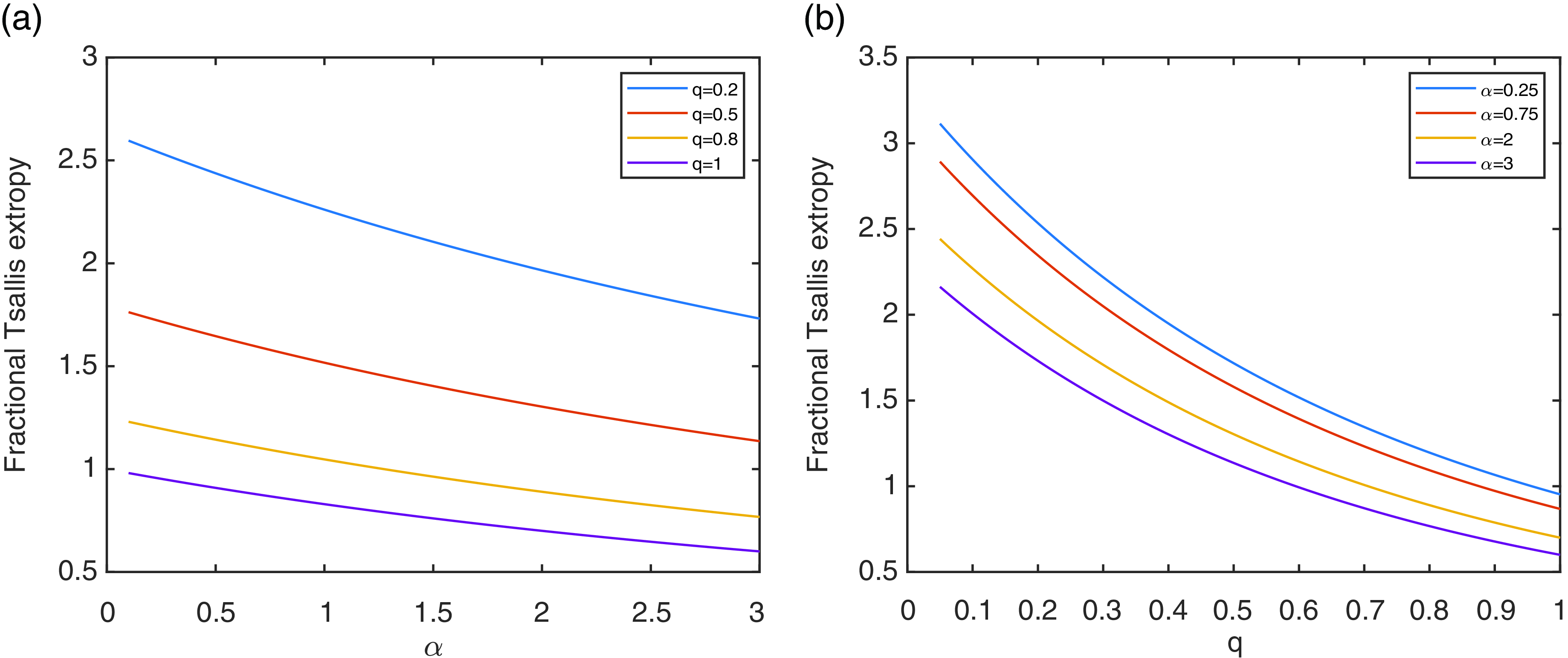
Figure 2. The fractional Tsallis extropy in Example 1 as a function of $\alpha$
for different choices of q (a), and as a function of q for different choices of
$\alpha$
for different choices of q (a), and as a function of q for different choices of $\alpha$
(b).
$\alpha$
(b).
Table 1. Values of the fractional Tsallis extropy for the discrete uniform distribution as a function of N, for different choices of q and $\alpha$
.
$\alpha$
.


Figure 3. The fractional Tsallis extropy in Example 2 as a function of N with different choices of the parameters $\alpha$
and q.
$\alpha$
and q.
4. A unified formulation of extropy
Now we introduce a unified formulation of extropy in the context of the Dempster–Shafer theory of evidence via
 \begin{align}JD_{\alpha}^q(m)= \dfrac{1}{\alpha-1}\sum_{A\subset X\colon m(A)>0} (1-m(A))\biggl[1-\biggl(\dfrac{1-m(A)}{2^{|A^c|}-1}\biggr)^{\alpha-1}\biggr]\biggl(\!-\!\log \dfrac{1-m(A)}{2^{|A^c|}-1}\biggr)^{q-1},\end{align}
where $\alpha>0$
,
$\alpha>0$
, $\alpha\ne1$
, and
$\alpha\ne1$
, and $0<q\leq1$
. As well as the fractional Tsallis extropy, this is a general formulation, since it includes several versions of extropy measures in the context of both DST and classical probability theory.
$0<q\leq1$
. As well as the fractional Tsallis extropy, this is a general formulation, since it includes several versions of extropy measures in the context of both DST and classical probability theory.
Remark 3. The unified formulation of extropy (8) is also non-negative.
Proposition 4.
If $q=1$
, the unified formulation of extropy in (8) is equal to Tsallis–Deng extropy in (5).
$q=1$
, the unified formulation of extropy in (8) is equal to Tsallis–Deng extropy in (5).
Proof. By taking $q=1$
in (8), we have
$q=1$
in (8), we have
 \begin{equation}JD_{\alpha}^1(m)=\dfrac{1}{\alpha-1}\sum_{A\subset X\colon m(A)>0} (1-m(A))\biggl[1-\biggl(\dfrac{1-m(A)}{2^{|A^c|}-1}\biggr)^{\alpha-1}\biggr]=JD_{\alpha}(m).\end{equation}
Proposition 5.
The unified formulation of extropy in (8) converges to the fractional Deng extropy in (4), as $\alpha$
goes to 1.
$\alpha$
goes to 1.
Proof. By taking the limit for $\alpha$
going to 1 in (8), and by using L’Hôpital’s rule, it follows that
$\alpha$
going to 1 in (8), and by using L’Hôpital’s rule, it follows that
 \begin{align*}\lim_{\alpha\to1}JD_{\alpha}^q(m)&= \lim_{\alpha\to1}\sum_{A\subset X\colon m(A)>0} (1-m(A))\biggl[\biggl(\dfrac{1-m(A)}{2^{|A^c|}-1}\biggr)^{\alpha-1}\biggr]\biggl(\!-\!\log \dfrac{1-m(A)}{2^{|A^c|}-1}\biggr)^{q} \\[5pt] &= \sum_{A\subset X\colon m(A)>0} (1-m(A))\biggl(\!-\!\log \dfrac{1-m(A)}{2^{|A^c|}-1}\biggr)^{q}\\[5pt] &=JD^q(m),\end{align*}
and the proof is complete.
Corollary 2.
When both parameters $\alpha$
and q in (8) tend to 1, the unified formulation of extropy in (8) converges to Deng extropy in (3), that is,
$\alpha$
and q in (8) tend to 1, the unified formulation of extropy in (8) converges to Deng extropy in (3), that is,
 \begin{equation*}\lim_{\alpha,q\to1} JD_{\alpha}^q(m)=JD(m).\end{equation*}
Remark 4. If the BPA m is such that all focal elements have cardinality $N-1$
, then in the expression of the unified formulation of extropy,
$N-1$
, then in the expression of the unified formulation of extropy, $|A^c|=1$
for each term in the sum. Hence the unified formulation of extropy reduces to
$|A^c|=1$
for each term in the sum. Hence the unified formulation of extropy reduces to
 \begin{align*}JD_{\alpha}^q(m)&= \dfrac{1}{\alpha-1}\sum_{A\subset X\colon m(A)>0} (1-m(A))\bigl[1-(1-m(A))^{\alpha-1}\bigr][\!-\!\log (1-m(A))]^{q-1}\\[5pt] &= JS_{\alpha}^q(Y),\end{align*}
where Y is a discrete random variable with support $X=\{\theta_1,\ldots,\theta_N\}$
such that
$X=\{\theta_1,\ldots,\theta_N\}$
such that $p_i=\mathbb P(\theta_i)=m(X\smallsetminus\{\theta_i\})$
, for
$p_i=\mathbb P(\theta_i)=m(X\smallsetminus\{\theta_i\})$
, for $i=1,\dots,N$
.
$i=1,\dots,N$
.
To summarize the results given in Propositions 4 and 5, Corollary 2, and Remark 4, the relationships between different formulations of extropy are depicted in Figure 4 in the form of a schematic diagram.

Figure 4. Relationships between different entropies in DST (blue) and classical probability theory (yellow).

Figure 5. The unified formulation of extropy in Example 3 as a function of $\alpha$
for different choices of q (a), and as a function of q for different choices of
$\alpha$
for different choices of q (a), and as a function of q for different choices of $\alpha$
(b).
$\alpha$
(b).
Theorem 2.
The supremum of the unified formulation of extropy in (8), as a function of $q\in(0,1]$
, is attained at one of the extremes of the interval, and the infimum is either attained at one of the extremes of the interval or it is a minimum at a unique
$q\in(0,1]$
, is attained at one of the extremes of the interval, and the infimum is either attained at one of the extremes of the interval or it is a minimum at a unique $q_0\in(0,1)$
.
$q_0\in(0,1)$
.
Proof. The proof is similar to that of Theorem 1.
Example 3. Let X be a frame of discernment with cardinality 4 and consider the BPA $m^*$
such that
$m^*$
such that
 \begin{equation*}m^*(A)=\dfrac{2^{|A|}-1}{\sum_{B\subseteq X} (2^{|B|}-1)}, \quad A\subseteq X.\end{equation*}
It is a well-known BPA which gives the same mass to all the subsets with the same cardinality. More precisely, with $|X|=4$
, we have four subsets with cardinality 1 and mass
$|X|=4$
, we have four subsets with cardinality 1 and mass $1/65$
, six subsets with cardinality 2 and mass
$1/65$
, six subsets with cardinality 2 and mass $3/65$
, four subsets with cardinality 3 and mass
$3/65$
, four subsets with cardinality 3 and mass $7/65$
, and one subset with cardinality 4 and mass
$7/65$
, and one subset with cardinality 4 and mass $15/65$
. Remember that the last one, i.e. the entire frame of discernment X, is not involved in the evaluation of the unified formulation of extropy. In Figure 5, the values of the unified formulation of extropy of
$15/65$
. Remember that the last one, i.e. the entire frame of discernment X, is not involved in the evaluation of the unified formulation of extropy. In Figure 5, the values of the unified formulation of extropy of $m^*$
are plotted as a function of
$m^*$
are plotted as a function of $\alpha$
or q.
$\alpha$
or q.
4.1. Application to classification problems
The measures of uncertainty are an efficient tool in the classification problems; see, for instance, [Reference Balakrishnan, Buono and Longobardi1], [Reference Balakrishnan, Buono and Longobardi2], and [Reference Buono and Longobardi3]. Here the unified formulation of extropy is applied to the classification problem based on the Iris flowers dataset given in [Reference Dua and Graff8]. It is composed of 150 instances equally divided into three classes, Iris setosa ( $\operatorname{Se}$
), Iris versicolor (
$\operatorname{Se}$
), Iris versicolor ( $\operatorname{Ve}$
), and Iris virginica (
$\operatorname{Ve}$
), and Iris virginica ( $\operatorname{Vi}$
), and, for each of them, four attributes are known, i.e. the sepal length in cm (SL), the sepal width in cm (SW), the petal length in cm (PL), and the petal width in cm (PW). By using the method of max–min values, the model of interval numbers is obtained and is presented in Table 10 in [Reference Balakrishnan, Buono and Longobardi1]. Suppose the selected instance is
$\operatorname{Vi}$
), and, for each of them, four attributes are known, i.e. the sepal length in cm (SL), the sepal width in cm (SW), the petal length in cm (PL), and the petal width in cm (PW). By using the method of max–min values, the model of interval numbers is obtained and is presented in Table 10 in [Reference Balakrishnan, Buono and Longobardi1]. Suppose the selected instance is $(6.3, 2.7, 4.9, 1.8)$
. It belongs to the class Iris virginica and our purpose is to classify it correctly. Four BPAs, one for each attribute, are generated by using the similarity of interval numbers proposed by Kang et al. [Reference Kang, Li, Deng, Zhang and Deng9]. Without any additional information, the final BPA is determined by giving the same weight to each attribute. In order to discriminate between classes, we evaluate the PPT (2) of singleton classes for the final BPA obtaining
$(6.3, 2.7, 4.9, 1.8)$
. It belongs to the class Iris virginica and our purpose is to classify it correctly. Four BPAs, one for each attribute, are generated by using the similarity of interval numbers proposed by Kang et al. [Reference Kang, Li, Deng, Zhang and Deng9]. Without any additional information, the final BPA is determined by giving the same weight to each attribute. In order to discriminate between classes, we evaluate the PPT (2) of singleton classes for the final BPA obtaining $\operatorname{PPT}(\operatorname{Se})=0.1826$
,
$\operatorname{PPT}(\operatorname{Se})=0.1826$
, $\operatorname{PPT}(\operatorname{Ve})=0.4131$
,
$\operatorname{PPT}(\operatorname{Ve})=0.4131$
, $\operatorname{PPT}(\operatorname{Vi})=0.4043$
. Thus the focal element with the highest PPT is the class Iris versicolor, which would be our final decision but which is not the correct one. Hence we try to improve the method by using the unified formulation of extropy in (8), by choosing as parameters
$\operatorname{PPT}(\operatorname{Vi})=0.4043$
. Thus the focal element with the highest PPT is the class Iris versicolor, which would be our final decision but which is not the correct one. Hence we try to improve the method by using the unified formulation of extropy in (8), by choosing as parameters $q=0.5$
and
$q=0.5$
and $\alpha=5$
. The unified formulation of extropy of BPAs obtained by using the similarity of interval numbers is evaluated and the corresponding results are given in Table 2.
$\alpha=5$
. The unified formulation of extropy of BPAs obtained by using the similarity of interval numbers is evaluated and the corresponding results are given in Table 2.
Table 2. The unified formulation of extropy of BPAs based on similarity of interval numbers.

A greater value of the unified formulation of extropy represents a higher uncertainty, so it is reasonable to give more weight to the attributes with a lower value of that measure. Here we define the weights by normalizing to 1 the reciprocal values of the unified formulation of extropy, and the results are given in Table 3.
Table 3. The weights of attributes based on the unified formulation of extropy.

Based on the weights in Table 3, a weighted version of the final BPA is obtained. Then the PPTs of the singleton classes are computed as $\operatorname{PPT}(\operatorname{Se})=0.1156$
,
$\operatorname{PPT}(\operatorname{Se})=0.1156$
, $\operatorname{PPT}(\operatorname{Ve})=0.4360$
,
$\operatorname{PPT}(\operatorname{Ve})=0.4360$
, $\operatorname{PPT}(\operatorname{Vi})=0.4485$
. Hence the focal element with the highest PPT is the type Iris virginica, and it would therefore be our final decision, which is the correct one. By using the method based on the unified formulation of extropy, a gain in terms of recognition rate is obtained going from 94% of the non-weighted method to
$\operatorname{PPT}(\operatorname{Vi})=0.4485$
. Hence the focal element with the highest PPT is the type Iris virginica, and it would therefore be our final decision, which is the correct one. By using the method based on the unified formulation of extropy, a gain in terms of recognition rate is obtained going from 94% of the non-weighted method to $94.67\%$
of the method explained here.
$94.67\%$
of the method explained here.
5. Conclusions
The recent study of the extropy as a dual measure of uncertainty has inspired us to introduce its unified formulation. We have obtained well-known concepts of extropy for particular choices of the two parameters involved. This unified formulation has also been analyzed in the context of the Dempster–Shafer theory of evidence. Further, an application to classification problems of the proposed measure is described.
Acknowledgements
The authors thank the Editor-in-Chief and the anonymous reviewers for their insightful comments and suggestions, which have helped to improve the quality of the manuscript. Francesco Buono and Maria Longobardi are members of the research group GNAMPA of INdAM (Istituto Nazionale di Alta Matematica) and are partially supported by MIUR – PRIN 2017, project ‘Stochastic Models for Complex Systems’, no. 2017 JFFHSH.
Funding information
There are no funding bodies to thank relating to this creation of this article.
Competing interests
There were no competing interests to declare which arose during the preparation or publication process of this article.


