


1. Introduction
One of the most striking features of the ice-core records from Greenland is a sudden drop in oxygen-isotope values (δ 18O) between roughly 12 000 and 11 000 years ago. This Younger Dryas event was an intense return to ice-age conditions during a lime of general deglaciation. As recorded in the ice cores, temperatures in Greenland cooled by roughly 7 K.
Reference Broecker and DentonBroecker and Denton 1989) and Reference FairbanksFairbanks (1989) have proposed competing explanations for the cooling and cause of this “aborted ice age”. One supposes that the 7 deg cooling is real and results from a shut-down in the North Atlantic Ocean circulation; the other, that it is largely fictitious and records an intrusion of isotopically light glacial meltwater into the ice-core records.
Due to its great thickness, the temperatures within the Greenland ice sheet have a memory of the past climate. In principle, those temperatures should provide an independent record of the past surface temperature. That record might help resolve the controversy.
In a seminal study, Reference Dahl-Jemen and JohnsenDahl-Jensen and Johnsen (1986) used a simple heat-flow model to reproduce the temperatures measured in the Dye 3 borehole in south central Greenland. Through trial and error, they were able to construct a simple temperature history showing many of the known temperature changes of the last few millennia. Reference MacAyeal, Firestone and WaddingtonMacAyeal and others (1991) repeated the analysis using more aggressive optimal control methods in the hope of detecting temperature changes around the lime of the Younger Dryas. They obtained a very close match to the measurements and a detailed surface-temperature history with an apparent Younger Dryas event consistent with Fairbanks’s explanation.
The temperature history, however, is troubled by severe oscillations that may distort, obscure or exaggerate the paleoclimate information contained in the measurements. The authors ’ paper was intended as a tutorial introducing the control method; it was not meant to be a convincing resolution of the controversy. “Whether [the history] supports the possibility of a Younger Dryas event in Greenland”, remarked the authors, “remains to be established”.
In his Ph.D. thesis, Reference FirestoneFirestone (1992) sought to refine the control method and convincingly answer the question: is it possible to resolve the Younger Dryas event through borehole thermometry? Although recent studies have changed the nature of the original Younger Dryas controversy (cf. e.g. Reference Charles and FairbanksCharles and Fairbanks, 1992; Reference JohnsenJohnsen and others, 1992; Reference Lehman and KeigwinLehman and Keigwin, 1992), the ideas and methods involved in answering this question are still exciting. This paper presents the author’s Ph.D. thesis in condensed form.
2. A Heat-Flow Model
To resolve the Younger Dryas event through borehole thermometry first requires a heat-flow model. The model is a reduced version of the finite-element model Reference Firestone, Waddington and CunninghamFirestone and others (1990) applied at the Summit ice divide, central Greenland. The model solves the two-dimensional, time-dependent heat-flow equation

where x is along the direction of ice flow, z is positive upwards, u and w are the velocity components in those same directions, T is the temperature, t is the time, ρ, c and K are the density, heat capacity and conductivity, and finally, f is the heat of deformation.
The model represents the combined ice and firn at Dye 3 as 2000 m of ice-equivalent. The model assumes no melting at the ice-bedrock interface and includes a 3000 m thick layer of bedrock below the ice to model the effects of bedrock thermal inertia.
The model decouples the heat and ice-flow equations. It assumes the thickness of the ice sheet has not changed over time and that the ice velocities assume a fixed profile determined from: observed tilting of the Dye 3 borehole, a simple velocity model and the age depth relation measured in the Dye 3 ice core.
The model assumes the heat flow at Dye 3 is linear (i.e. ρ, c and K arc constant) and primarily one-dimensional. The model solves for heat conduction and advection in the vertical but includes the effects of strain heating and horizontal heat advection. The model uses three-node, quadratic, one-dimensional finite elements, three-point Gaussian quadrature and a fully implicit time-stepping scheme.
At the bottom of the 3000 m of bedrock, I introduce a constant geothermal heat flux. At the ice-sheet surface, I apply a time-dependent temperature or heat-flux forcing. I step the model through time and scale the fixed velocity pattern to a simple mass-balance history (Reference Paterson and WaddingtonPaterson and Waddington, 1986, Fig 1).

Fig. 1. The present-day borehole-temperature response to a step change in surface temperature applied at various times in the past. The responses shown are for step changes at 208, 416, 649, 996, 1522, 2317, 3516, 5237, 8062, 12199, 18447 27886, 42148. 63699, 96262, 145459, 219 789, 332095 and 501779 year BP. The shaded region shows responses from roughly the last deglaciation.
3. Some Fast Science
The isotope values recorded in the Dye 3 ice core suggest that Greenland cooled roughly 7 K during the Younger Dryas (Reference Dansgaard, White and JohnsenDansgaard and others, 1989). As a first test of the model, I apply a glacial/interglacial temperature forcing (Reference Paterson and WaddingtonPaterson and Waddington, 1986, Fig 1) with a present-day temperature of-20.1 °C and an ice-age temperature 12 K colder than today. I run the model through a number of glacial cycles to make the model “forget” its initial condition. During the last cycle, I add a 7 K cooling between 11 500 and 10 700 year BP to simulate a Younger Dryas cooling event, I find that at no time does the ice sheet reach the melting point and that remnants of a Younger Dryas cooling should appear in today’s borehole temperatures as roughly 0.2 K of added cooling near the bed of the ice sheet.
Ice-sheet temperature observations typically have an accuracy of ~10mK, an order of magnitude smaller. In principle, it should be possible to detect a cooling during the Younger Dryas in the temperatures measured at Dye 3. In practice, the cooling may not be resolvable. Thermal diffusion makes the temperatures measured today an average of the past temperature; noise in the temperature observations and models make solutions of the ice-sheet temperature problem non-unique. Consequently, there are an infinite number of temperature histories that will match the Dye 3 borehole observations within their error. The cooling during the Younger Dryas may have been too short to distinguish unambiguously from other smaller and more recent temperature changes. To prove convincingly or disprove a cooling, I must show that these more recent changes cannot explain the observations.
Resolving the Younger Dryas event in the Dye 3 borehole, temperatures will be a subtle proposition. From a space of possible forcings, I must choose a particular forcing or set of forcings that “best” explain the observations in some sense. To prove convincingly or disprove a Younger Dryas cooling, I will develop objective methods that find an “optimum” surface-temperature history from the temperatures observed today. Before I describe those somewhat complicated methods, 1 perform some quick and simple sensitivity tests, some fast science, to establish the rough boundaries of the solution space.
I start the heat-flow model at some time in the past and apply a single surface-temperature step change. I run the model and follow the response of the ice sheet’s temperature field up to the present day. I repeal this process starting at other times and obtain present-day temperature responses for a range of past surface-temperature step changes.
Figure 1 shows the responses I obtain. The shaded part shows the responses from step changes during the last deglaciation. The effect of vertical advection is most impressive. It concentrates in the bottom third of the ice sheet the response from surface-temperature changes around the time of the Younger Dryas and it transports into the ice sheet’s bed, roughly one-half the response from a step change at 18 000 year BP. The concentration of the responses into the lower third of the ice sheet suggests that different temperature changes around the time of the Younger Dryas event may produce responses with only slight differences. It may be difficult to discern the event’s precise onset and duration.
Next, I trace the half-response heights shown in Figure 1. I obtain a temperature-change “time-scale” (Fig. 2. solid line): the age of the surface-temperature spike that registers a peak response at each depth in the Dye 3 borehole. I compare this against a time-scale I determine from the Dye 3 ice-core isotope values (Fig. 2, dashed line). The two generally agree. This confirms that surface temperature changes at Dye 3 are propagated principally by advection and that the model’s vertical velocity profile was derived from the Dye 3 ice-core time-scale.

Fig. 2. The Dye 3 ice-core time-scale (dashed line) compared against the Dye 3 temperature-change time-scale: the age of the surface-temperature spike whose peak response is at a given depth (solid line). Near the surface and near the bed. heat conduction propagates temperature changes more rapidly than advection. Consequently, the temperature-change time-scale begins slightly lower than the ice-core time-scale, and then further diverges below 250 m.
Vertical advection determines the ice-core time-scale, whereas both vertical advection and conduction determine the temperature-change time-scale. Near the surface, heat conduction propagates changes more rapidly than advection. Consequently, the temperature-change time-scale starts off slightly lower than the ice-core time-scale. Approaching the bed, the vertical velocity at Dye 3 rapidly decreases to zero. Heat conduction again propagates changes more rapidly, causing the temperature-change and ice-core time-scales to diverge further.
The divergence of the time-scales starts around 10 000 year BP. This suggests that mass-balance changes during and after the Younger Dryas will have a greater effect on the borehole-temperature response than mass-balance changes before. Temperature histories for Dye 3 should therefore be less sensitive to earlier ice-age mass-balance changes. This may improve the prospects for resolving the Younger Dryas event as those changes can be considerable.
Since the heat-flow model is linear, I ran difference the responses shown in Figure 1 and synthesize the response to a surface-temperature pulse of arbitrary width at an arbitrary time. From such an analysis, I can determine which borehole observations I need consider to detect and distinguish a possible Younger Dryas cooling. Assuming a χ2 detectabilily criterion, I find that I can disregard the temperature observations in the upper 300 m of the Dye 3 borehole, assuming those observations have a noise level of around 10 mK. I therefore confine my analysis to the temperatures between 0 and 1700 m above the bed.
By the same analysis, 1 determine the shortest surface-temperature pulse that should be detectable in the Dye 3 borehole temperatures, assuming observations having different noise levels, σ (Fig. 3). For a 10 k surface-temperature cooling and observations with 10 mK of noise, the shortest detectable pulse is given by the σ = 0.001 curve of Figure 3. For a 7 k cooling around the time of the Younger Dryas, the shortest detectable pulse is on the order of 100 years. The Dye 3 ice-core record suggests that the Younger Dryas event lasted about 5-7 times longer. Thus, it should seem possible to detect a Younger Dryas cooling in the present-day Dye 3 borehole temperatures.

Fig. 3. The shortest surface-temperature pulses detectable in the Dye 3 borehole temperatures at observation noise levels of 0.001, 0.01 and 0.1. Variations caused by the assumed ice-sheet surface-precipitation history (dashed line) appear in the curves for all noise levels. Strong numerical interpolation noise appears in the curve for an 0.001 noise level.
4. Least-Squares Minimization
I will now examine the Dye 3 borehole temperatures measured in 1983 and 1986 (Reference Gundestrup and HansenGundestrup and Hansen, 1984; Reference Hansen and GundestrupHansen and Gundestrup, 1988). From those temperatures, I will try to find the essential surface-temperature history implied by the simple heat-flow model. I will compare this history against the Dye 3δ180 record (Reference Dansgaard, Clausen, Gundestrup, Johnsen, Rygner, langway, Oeschger and DansgaardDansgaard and others, 1985) and try to answer: do the low isotope values during the Younger Dryas reflect a marked cooling or do they indicate something else?
To find the essential history and produce a convincing answer, I make the classical statistical assumptions regarding the data and carry out a least-squares/ maximum likelihood analysis. I estimate variances for the data, ![]() and form the χ2 mismatch between the temperatures measured in the Dye 3 borehole,
and form the χ2 mismatch between the temperatures measured in the Dye 3 borehole, ![]() , and the terminal (present-day) borehole temperatures,
, and the terminal (present-day) borehole temperatures, ![]() , calculated by the simple heat-flow model
, calculated by the simple heat-flow model

Using a variable metric (quasi-Newton) optimization program (Reference Press, Flannery, Teukolsky and VetterlingPress and others, 1986, section 10.7), I minimize Equation (2). I run the heat-flow model with various surface-temperature histories until I find the history that produces borehole temperatures that most closely match the observations. To speed convergence to a minimum, the optimization program considers the gradient of the mismatch with respect to the forcing. In the first minimizations, I calculate the gradient by finite differences.
For efficiency, I reduce the size of the simple heat-flow model’s spatial and temporal mesh while being careful to preserve the accuracy of the model. Using simple sensitivity tests, I find a finite-element mesh with nodes spaced further apart where the borehole temperatures vary less rapidly. I also determine a set of 1400 unequally spaced time steps between 675 and 0 kyear BP (Fig. 4) that are consistent with the shortest surface-temperature pulse detectable in the Dye 3 borehole temperatures (Fig. 3).

Fig. 4. The placement and sizes of the 1400 model time steps determined through a “fast science” analysis of Figure 3.
A temperature change over each of these “equal-influence” time steps yields an equal χ 2 response in the model’s terminal temperatures. This fixes the “regularizaron” of the solution, the amount of variation I allow in the surface-temperature solution over each interval of time. As Figure 4 shows, I allow recent parts of the solution to vary more rapidly. In this way, I account for the greater information (more detailed variations) recorded in the upper borehole temperatures (cf. Reference FirestoneFirestone, 1992, chapter 5, appendix A).
To begin, I find simple temperature histories and geothermal heat-flux values consistent with the borehole temperature measured in 1983. (This section combines sections 4.3 and 5.3 of the thesis (Reference FirestoneFirestone, 1992).) I apply to the model: a geothermal heat flux, a simple temperature history inspired by the Dye 3δ18O record, and the simple precipitation pattern of Figure 3 scaled to have minimum ice-age precipitation rates of one-half, one-third or one-fifth of today’s value. I run the optimization program and heat-flow model to find surface-temperature histories and geothermal heat-flux values that best match the 31 borehole observations between 0 and 1700 m.
I obtain geothermal heat-flux values and simple histories (Fig. 5) that agree with results quoted previously (e.g. Reference Dahl-Jemen and JohnsenDahl-Jensen and Johnsen, 1986). The values suggest that air temperatures in Greenland were roughly 2 k warmer during the climatic optimum and 12-16 k colder during the last ice age.

Fig. 5. The model parameters determined in the first minimizations: the most likely geothermal heat-flux values and simple surface-temperature histories that match the 1983 Dye 3 temperature observations, assuming the precipitation pattern of Figure 3 and minimum ice-age precipitation rates of one-half, one-third and one-fifth of today’s value.
At depth, the residuals produced in the three minimizations (Fig. 6) generally fall within the quoted accuracy of the 1983 observations, 0.03 k (Reference Gundestrup and HansenGundestrup and Hansen. 198 Ii. Approaching the surface, the residuals show large and regular biases. These result from more recent surface-temperature changes omitted from the simple surface-temperature histories.

Fig. 6. The mismatches between the 1983 Dye 3 temperature observations and the terminal model temperatures produced by the three simple, temperature histories of Figure 5. The mismatches are almost indistinguishable, probably because the assumed precipitation pattern and calculated surface-temperature histories follow the same pattern. The dashed lines show the estimated, worst-case accuracy of the observations.
5. Optimal Control
After making these “most likely” fits, there remain slight biases in the residuals below 1000 m. The 1983 data set is too small and too inaccurate to recognize these as remnants of a Younger Dryas cooling. Fortunately, there exist the several thousand temperatures measured in 1986. 1 combine these with the 1983 observations to form a much larger and accurate data set.
Hope for discerning the Younger Dryas in these combined borehole temperatures rests with explaining the remaining biases by additional ancient surface-temperature variations and then demonstrating that those variations are necessary. The difficulty in this is that the ice-sheet heat-flow problem is “ill-posed”. In order to obtain a stable solution, I must place constraints on it, These constraints are largely arbitrary, and consequently, to some degree, so is any solution I obtain.
In the first minimizations, I forced the surface-temperature history to have a very simple, five-kink variation, and thus made the heat-flow problem well-posed. I now want to find a more complicated history to explain the residuals left by the first minimizations. In the spirit of Occam’s razor (Reference Constable, Parker and ConstableConstable and others, 1986), I will seek a more complicated history that is still the simplest possible that explains the observations. To allow the solution the greatest possible freedom of expression, I make the surface temperature forcing over each time step, an unknown in the minimizations. Then, I force this detailed solution to be simple by penalizing its departure from one of the simple, five-kink surface-temperature solutions of Figure 5.
To simplify the mathematics, I apply and manipulate heat-flux forcings rather than temperatures. I apply a flux forcing at the surface rather than a temperature history. I then encourage the flux forcing to resemble the surface-flux equivalent of the simple, five-kink history. I append to the observation-model mismatch Equation (2) the χ 2 mismatch of the detailed surface-flux forcing and the simple five-kink history. I produce the performance function:

where Q f is the basal and surface-flux forcing, P is the flux-forcing equivalent to the five-kink temperature history, and S p arc the variances I assign to this simple, flux-forcing “pre-conception”. The “regularization” parameter, ∈ specifies how much I penalize the departure of the detailed solution from the simple preconception.
I find detailed solutions that best match the observations using the variable metric optimization program. I must supply to this program the gradient of the performance function, L, with respect to each forcing variable, about 1401 values. The cost of calculating this gradient by finite differences is prohibitive. However, I can reduce the cost by three orders of magnitude if I recast the calculation of the gradient as a problem in optimal control.
I introduce vectors of Lagrange undetermined multipliers, λ(m), one set for each time step, and I define an augmented performance function to minimize (Reference Thacker and LongThacker and Long, 1988). To Equation (3), I add the heat-flow model as a constraint. I obtain:

The terms within curly braces represent the heat-flow model at times m = 0, …, M where C(m) is the “thermal mass” (heat capacity) at time m, K(m) the “thermal stiffness” (thermal conductivity), Q(m) the nodal heat-flux forcings and R(m) the nodal heat sources due to horizontal advection and strain heating.
I find the minimum of the augmented performance function, L′, by taking its variation with respect to the unknown Lagrange multipliers, λ(m), the model state variables, T(m) and the model forcings, Q f. I obtain, respectively, the original heat-flow model, Equation (5); its adjoint, Equation (6) and Equation (7); and the gradient of the performance with respect to the 1401 flux-forcing values, Equation (8):


In Equations (6) and (8), the terms ![]() and
and ![]() represent the terminal temperature/nodal temperature Jacobian and the nodal flux/flux-forcing Jacobians.
represent the terminal temperature/nodal temperature Jacobian and the nodal flux/flux-forcing Jacobians.
Starting with a first guess for the flux forcing, I solve these equations, in turn. From Equation (5), I obtain a first match to the data; from Equation (6), the initial condition of the adjoint trajectory (Reference Thacker and LongThacker and Long, 1988); from Equation (7), its evolution backwards in time; and from Equation (8), the gradient leading to a closer match. I feed to the optimization program the performance of the first guess Equation (4) and its gradient Equation (8). The program then tests and obtains a second, improved guess. I repeat this process for the second guess, and for successive guesses, until I find the simplest flux forcing that produces the best match to the observations. I define “simplest” and “best matches” by the second and first terms of Equation (4). Ft ’om the temperatures calculated for the model’s surface node, I obtain the equivalent surface-temperature forcing.
6. Resolving The Younger Dryas Event
Having constructed a suitable heat-flow model, chosen flexible model forcings, calculated a simple solution to use as a preconception and established efficient means to find a simplest, best-matching solution, 1 shall now try to determine the essential climate history recorded in the Dye 3 temperature data.
A first, detailed, “unconstrained” minimization demonstrates that the borehole data poorly constrain the surface temperatures over the last glacial cycle. Therefore, I impose as a preconception, the temperatures from the simple solutions before 14 984 year BP. As a first attempt, I give the preconceptions fairly high weight (∈ = 1000). By the procedure just described, I find forcing solutions that are close to the simple preconceptions prior to 14 984 year BP and that produce terminal model temperatures that are closest to the 1983-86 temperature observations.
I obtain the geothermal heat-flux values of before and terminal model temperatures that more closely match the Dye 3 observations. Figure 7 shows the mismatch assuming an ice-age precipitation rate one-third today’s value. (The mismatches for the two other precipitation histories look similar.) Above 200 m height, the residuals largely fall within the most optimistic error bands I can assign to the data. The residuals show rapid milli-degree oscillations and short spikes. The former probably represent data-logger digitization noise, and the latter, temperature-step changes caused by thermal convection cells in the borehole Quid Hansen and Gundestrup, 1988).

Fig. 7. The mismatch between the 1983 86 Dye 3 temperature observations and the terminal model temperatures produced in the constrained minimization, assuming an ice-age precipitation rate one-third of today’s value. The dashed lines show the estimated, best-case accuracy of the observations. Precipitation histories with ice-age precipitation rates one-half and one-fifth of today’s value yield similar mismatches.
The residuals at 0 and 16 m height are roughly 0.03 and 0.07 k too warm and fall outside the most optimistic error bands. This may be due to biases in the model fits caused by: poor physics, numeric ringing in the temperature solution or severe instrumentation noise that existed in the 1983 data-logging system personal communication from N.S. Gundestrup, 1991).
Figure 8a shows the surface-temperature histories I obtain. Starting at 675 000 year BP. the forcings closely follow the preconceptions until the preconceptions end at 14 984 year BP. At 14 984 year BP, the temperatures jump to warmer values; around the time of the Climatic Optimum they reach their maximum values, 1.8-2.1 k warmer than today. The peak temperature shifts slightly and changes value depending on the assumed ice-age precipitation rate.

Fig. 8. The detailed surface-temperature histories that produced the mismatch shown in Figure 7 (or something similar). The older parts of the histories (panel a, chained lines) closely follow the forcing preconceptions to their end at 14 984 year BP. The recent parts (panel b) show the Climatic Optimum and an early medieval warming.
Figure 8b shows the recent surface-temperature histories in greater detail. After peaking at 4500 4000 year BP, the temperatures smoothly and gradually decrease to today’s value, while slightly warming during the “medieval” period around 1500 year BP.
The temperature histories show no evidence of a Younger Dryas cooling. This could be because the cooling did not occur. Alternatively, the temperature data sets, from which I determined the histories, may contain too little information for the model to distinguish it. To test the latter hypothesis, that the observations are insufficient, I suppose that the Dye 3 temperature observations indicate that the Younger Dryas cooling had not occurred.
Using the heat-flow model, I synthesize the changes that would appear in the Dye 3 borehole temperatures had a 7 k cooling occurred during the Younger Dryas. I add the synthetic changes to the observations, run more minimizations and try to detect this synthetic cooling. First, I compute a set of preconceptions following the procedure of section 5 above.
Figure 9 shows the temperature histories and geothermal flux values I obtain and compares them to those I obtained earlier. Had something like a Younger Dryas cooling occurred, the geothermal flux value would have been 1 mWm−2 higher; while the surface temperatures would have been 1 k cooler during the last ice age, 0.4 k cooler at 9624 year BP and largely unchanged at later times.

Fig. 9. The geothermal keat-flux values and simple surface-temperature histories that best match the 1983 temperatures with an added Younger Dryas cooling pulse. For comparison, the figure shows the original flax values and temperature histories I Fig. 5) in light type and with dashed lines.
Figure 10 plots the residuals from the preconceptions with and without an added Younger Dryas cooling. To the accuracy at which I can draw lines on the page, they arc identical.
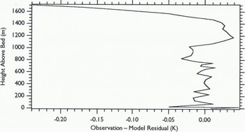
Fig. 10. The mismatch between the 1983 Dye 3 temperature observations with an added Younger Dryas cooling pulse and the terminal model temperatures produced by any of the six preconceptions of Figure 9. By slight adjustment of the geothermal heat-flux values and ice-age temperatures, the new preconceptions have removed nearly all traces of the Younger Dryas cooling pulse.
With just minor adjustments to the preconceptions, 1 have produced nearly identical matches to the Dye 3 observations. The final preconceptions leave no hint of a Younger Dryas cooling. There is little point in running a detailed minimization. With these minor adjustments, the new preconceptions have removed any residual that might have been left by a Younger Dryas cooling.
I can only conclude that I cannot detect a Younger Dryas event with the present Dye 3 temperature observations.
7. Prospects
If the temperatures in the Greenland ice sheet show any remnants of a Younger Dryas cooling, those remnants will be subtle and difficult to distinguish from observation and modeling errors. To identify the remnants in a set of borehole temperatures, and so say something about the Younger Dryas. will require more accurate observations, better models and a more refined uncertainty analysis.
On the first two counts, Dye 3 is not an ideal site to detect and resolve the Younger Dryas event. It often shows some surface melting in the summer, it is far from the ice divide and it has very rough bed topography upstream. The high accumulation rate at Dye 3 also severely compresses the climatic record from the last ice age to a thin layer near the bed. For these and other reasons, investigators have looked to central Greenland for more favorable drilling sites.
The GISP2 and GRIP groups have now drilled a pair of deep boreholes near the Summit ice divide (72 °18′. 37 °55′W) and have retrieved two detailed ice cores spanning several glacial cycles. Extensive geochemical analyses of the cores are now under way and within the next few years the temperatures in the two boreholes will be measured. To determine whether these observations might distinguish the Younger Dryas event, I conduct an identical twin experiment to determine the minimum observation accuracy needed to resolve the Younger Dryas at Summit.
I modify the model to have ice flow like at Summit Reference Schøtt, Waddington and RaymondSchott and others. 1992), an appropriate set of equal-influence time steps, and a liner spatial mesh. I run the model with a simple Younger Dryas cooling history and I obtain a set of terminal model temperatures which I call the “observations”. I minimize as before and obtain a surface-temperature history that best matches these synthetic observations. A sufficiently accurate model and proper procedure should produce a history from the “observations” that is an identical twin of the original.
Figure 11 shows the twin surface-temperature histories: the history that created the observations and the history I recover from them. Despite a very close match to the synthetic observations (better than 10 μK), the recovered history shows little indication of the Younger Dryas cooling. There is a general cooling of ~1 k between 15 000 and 9000 year BP. This is, however, less than the observed temporal and spatial uncertainties of the δ 18O records from Greenland. To test the Younger Dryas “cooling” in the Summit isotope values, we will need to recover a larger temperature change. On that basis, the identical twin experiment shows that the model 1 have just constructed is incapable of distinguishing a Younger Dryas event.

Fig. 11. The Younger Dryas cooling history that produced the synthetic Summit borehole observations and the recovered temperature history whose terminal temperatures most closely match them. The history shows little or no hint of the Younger Dryas cooling pulse.
Through several sensitivity tests. 1 find that this failure is due to numerical diffusion introduced by the model’s implicit time-stepping scheme. This diffusion adds roughly 3 mK of noise to the terminal model temperatures. Since the synthetic observations are terminal model temperatures, this implies that we will need to measure the borehole temperatures to much better than 3 mK accuracy.
Supposing that we can measure the temperatures at Summit to a much higher accuracy, we will then require a much more accurate and detailed model than I use here. Further sensitivity tests suggest that the model will need to include temperature-dependent thermal properties, two-dimensional heat flow and shorter-term precipitation-rate changes. It also will need to consider the effects of ice-flow pattern and ice-sheet thickness changes, and recent movements of the Summit ice divide.
To distinguish the Younger Dryas event will most likely require a coupled, thermo-mechanical model of the Summit ice divide with heat flow and ice (low responding to past changes in precipitation and temperature. Such a complicated model is feasible and it can be managed and brought into agreement with the observations by extending the optimal control methods presented here.
The results produced by such a model will require a better uncertainty analysis. We can obtain refined uncertainties through a straight-forward analysis of the Hessian produced in the optimizations.
8. Summary and Conclusions
The controversy surrounding the Younger Dryas event remains unresolved. Borehole thermometry was unable to distinguish the event at Dye 3 because the observations were too inaccurate. The prospects for Summit are more favorable but remain unclear. In principle, an improved model and more accurate observations may resolve the event. In practice, they may not because neither may ever be known in sufficient detail. Nonetheless, resolving the Younger Dryas event through borehole thermometry is still well worth attempting.
That claim may seem dubious. The chemical species in ice cores already provide a detailed record of the past climate. Furthermore, that record will always be much more detailed than any history we produce from a set of ice-sheet borehole temperatures, as those temperatures are the product of much greater diffusion. What, then, is the use of borehole thermometry? It may never be able to resolve the Younger Dryas event and, at best, all it might do is confirm the past climate found in the geochemical record.
The geochemical record, however, is not without its difficulties. Its values are the product of complicated, multistage processes that arc incompletely known and only partially calibrated.
In contrast, the temperature history implied by a set of borehole temperatures results from simpler, more readily described, geophysical heat flow and ice flow. While it may lack detail, the history is a more direct proxy of its supposed forcings. That directness may allow borehole thermometry to determine and explain past climate obscured by complicating effects in the isotopic records. This directness may suggest the complicating effects in those records as well.
As an example, Figure 12 compares the surface-temperature history determined from the 1983-86 Dye 3 temperatures against the δ 18O values from the Dye 3 ice core, after I have assigned the values a time-scale, averaged them and corrected them for elevation effects. The figure plots the δ 18O values as the temperatures implied by a recent calibration of δ 18O paleothcrmometer (Reference Johnsen, Dansgaard and WhiteJohnsen and others, 1989).

Fig. 12. The temperature history determined from the Dye 3 borehole temperatures (Fig. 8a) compared against elevation-corrected δ18O values from the Dye 3 ice core. The warmest ice-age temperature suggested by the borehole temperatures is considerably colder than the average temperature implied by the δ 18O values. Between 5500 and 400 year BP, the history implied by the borehole temperatures generally agree with the isotope values. The isotope values show short-term variations which may or may not reflect changes in surface temperature.
Between 5500 and 400 year BP, when the borehole-temperature history is well constrained, the two generally agree. Even after 40-45 year averaging, however, the δ 18O values show considerable short-term variations. From the values alone, it is not possible to determine whether these are air-temperature changes or the effects of some complication such as changes in precipitation source.
Borehole thermometry and a refined uncertainty analysis, however, successfully recover the general temperature variation. Removing this temperature signal from the δl8O values leaves a residual showing the magnitude and timing of non-temperature effects. Comparison of this residual against other proxy climatic records may help determine their cause.
The (δ 18O “paleothermometer” has not been calibrated except for temperature changes over fairly recent times (e.g. Reference JohnsenJohnsen, 1977; Reference Cuffey, Alley, Grootes and AnandakrishnanCuffey and others, 1992). It is probably unrealistic to assume that the observed presentelas relation between δ 18O and mean annual air temperature in Greenland has held at all times.
Over the last ice age, the borehole temperatures suggest average air temperatures that are considerably colder than the value implied by the δ 18O record. About 4deg of the difference is likely caused by the increase in the σ180 value of the ice-age ocean-source water. I bis leaves 2-5 deg of cooling unaccounted for. Several non-temperature effects may cause this failure of the δ18O paleothermometer. for example, changes in the annual distribution of precipitation during the ice age.
Except for large, long-term precipitation-rate changes, the borehole temperatures at Dye 3 arc largely insensitive to such non-temperature effects. Borehole thermometry may thus provide a more realistic calibration of the δ18O paleothermometer. It might suggest a better relation between the values and past air temperatures. After iixing the relation, borehole thermometry might then suggest a broader relation between the values and past climate changes; for example, it might suggest a sensitivity to past changes in precipitation seasonality.
The Younger Dryas event was introduced as an important climatic problem that requires answers for non-temperature effects. Though it is perhaps the most famous, these other problems show that it is not the only one of its kind. As one geophysical modeler is fond of remarking, an explanation for the Younger Dryas controversy may prove to be the “holy grail” of climate research. Borehole thermometry may never resolve the controversy. However, if an impossible quest leads us to understand these other problems better, then resolving the Younger Dryas event through borehole thermometry is worth trying, for no other reason than the answers we may encounter on the way.
Acknowledgements
I should like to thank B. Anderson. D. Dahl-Jensen, P. Grootes, N. Gundestrup. D. MacAyeal. J. Pederson, A. Rasmussen. C. Raymond and E. Waddington for many interesting conversations that contributed to this work. While working on this project. J had the pleasure of visiting the University of Copenhagen. 1 wish to thank the members of the Glaciology Group for their help and hospitality. Two anonymous reviewers offered many helpful suggestions, not all of which I could incorporate into the present work. Their thoughts will live future lives in another paper now in preparation.
Temperature data used in this work were graciously provided by N. Gundestrup. C. Schøtt-Hvidberg kindly provided Summit model velocities. Oxygen-isotope data were supplied by the World Data Center A for Glaciology, Boulder, Colorado. Funding for this work was provided by the University of Washington Gcophvs-ics Program and by the U.S. National Science Foundation under grants DPP 8613935, DPP 891498. DPP 8915924 and DPP 9024098. This is publication No. 823 of the Alfred-Wegener-Institut.


