


1 INTRODUCTION
VLBI observations of extragalactic sources at radio wavelengths are used to define the fundamental celestial reference frame, the International Celestial Reference Frame II (ICRF2; Ma et al. Reference Ma2009; Fey et al. Reference Fey2015). It is well known that due to limited observing capabilities the ICRF is much weaker in the southern hemisphere than in the northern one. In terms of nominal source positions, which are strongly correlated with the number of observations and sessions in which a source is observed, southern sources are much less precise than northern ones (e.g. Plank et al. Reference Plank, Lovell, Shabala, Böhm and Titov2015, Figures 7 and 8).
The AuScope VLBI array (Lovell et al. Reference Lovell2013) was built to address these issues. The new Australian antennas in Katherine (Ke, Northern Territory), Yarragadee (Yg, Western Australia), and Hobart (Hb, Tasmania) have been regularly participating in the international observing programmes coordinated by the International VLBI Service for Geodesy and Astrometry (IVS, Nothnagel et al. Reference Nothnagel, Artz, Behrend and Malkin2016). In parallel, the AUSTRAL observing programme (Plank et al. Reference Plank2017) was established, having the aim to optimally utilise the new VLBI infrastructure and further improve the results for the Australian region. The Warkworth 12-m antenna (Ww) also participates in the AUSTRAL programme. The high cadence as well as the fact that the AUSTRALs have typically more observations than the standard IVS experiments make them an important contributor when counting the total number of observations. This is shown in Figure 1, illustrating the cumulative number of all observations since 2012. By distinguishing between all sessions and all without the AUSTRALs, one clearly sees that the AUSTRALs have been continually increasing their contribution to the total number of observations, also causing a change in the overall rate.
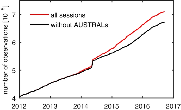
Figure 1. Cumulative number of all (red line) observations of the IVS from 2012 until 2016 September. For the black line, all sessions except the AUSTRAL sessions are considered. It is evident that the AUSTRAL sessions have become increasingly important, changing the overall rate of growth in the number of observations.
However, as the new and typically smaller telescopes are less sensitive than the existing array of IVS radio telescopes, this increase in the number of observations is highly dependent on the strength (respectively flux density) of the source. As illustrated in Figure 2, the distribution of observations amongst bins of source strengths is relatively balanced (≈20 000–40 000) for flux densities down to 0.6 Jy. For weaker sources, it rapidly falls off to about 13 000 observations for flux densities between 0.4 and 0.6 Jy and about 4 500 observations to sources between 0.2 and 0.4 Jy. In total, we find only about 1 500 observations in the AUSTRAL sessions to sources of a nominal flux density lower than 0.2 Jy.
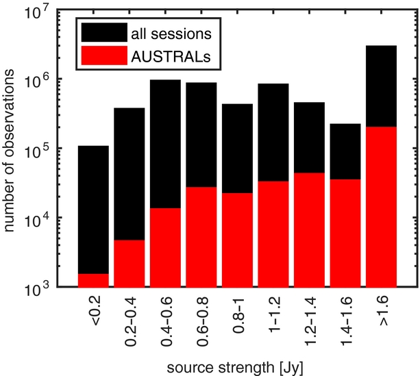
Figure 2. Cumulative IVS observations since 2012 (as shown in Figure 1) sorted in bins of sources with different flux densities (median values). While sources of all strengths are regularly observed in standard IVS sessions (all sessions are considered in the black bars), sources of flux densities lower than 0.6 Jy are significantly less frequently observed in the AUSTRAL sessions (red bars). Note the logarithmic scale.
In order to achieve better geodetic results through more observations, only strong sources are observed in the AUSTRAL sessions (Plank et al. Reference Plank2017). An exception are those sessions with an astrometric purpose or those with the addition of larger and thus more sensitive antennas to the array.
While the current procedure is fine for geodetic purposes, there is motivation to also include observations to weaker sources in the AUSTRAL programme:
-
• Maintaining the ICRF. All sources need to be re-observed regularly in order to monitor their flux densities and to allow a precise determination of their positions. The uneven distribution of position accuracies between the northern and southern sky is a problem and could be mitigated through more frequent observations in the south.
-
• Tie to the optical frame. Gaia, a mission by the European Space Agency, is expected to produce a new celestial reference frame at optical frequencies with unprecedented accuracies (http://sci.esa.int/gaia/). For aligning the optical frame to the ICRF, work has been done in identifying suitable ICRF2-Gaia transfer sources (Bourda et al. Reference Bourda, Charlot, Porcas and Garrington2010, Reference Bourda, Collioud, Charlot, Porcas and Garrington2011), both visible in the optical and radio domain, and including them in regular as well as in dedicated observing programmes of the IVS (Le Bail et al. Reference Le Bail2016). Once more southern sources are problematic to be regularly observed.
-
• Special sources. Due to their high cadence and flexibility in scheduling, the AUSTRAL sessions are also a very attractive option for monitoring special sources. These can be new sources, sources in a certain area used for phase referencing, and sources with a special characteristic or astrophysically interesting behaviour. Decreasing the flux density limit for such sources may increase the scientific output of the AUSTRAL sessions.
The most convenient possibility to increase the network sensitivity of the AUSTRALs is adding the Hobart26 antenna (Ho). Ho is co-located with the Hb telescope and like the AuScope array operated by the University of Tasmania (UTAS). However, when adding one large (i.e. more sensitive) antenna to a network of smaller ones does not necessarily help in scheduling weaker sources, without adapting the scheduling algorithm accordingly. For the particular network of the AUSTRAL sessions, a new strategy—the star mode—has now been developed and is introduced in this paper.
The idea, implementation, and application of this new mode to four AUSTRAL sessions are described in the following Section 2. In Section 3, results of the observations are given. In Section 4, a more general discussion about the new mode is given before concluding in Section 5.
2 STAR SCHEDULING MODE
Scheduling is the task of creating the observation plan, namely telling each antenna which source shall be observed at what time and for how long. This is a complex task, trying to solve multiple optimisation problems depending on the target of a session. Before describing the newly developed star mode algorithm in Section 2.2, an introduction to the basic relations in scheduling is given in the following section.
2.1. Scheduling basics
For a successful observation, the correlation signal of the recorded data at two sites observing an identical source should be strong enough enabling a clear detection. In scheduling, the scan length (t) of an observation is planned so that the source signal-to-noise ratio (SNR) becomes greater than a certain low limit SNR, where this limit is typically 20 for the X-band and 15 for the S-band. The scan length is calculated as the product of the antenna sensitivities (given by the system equivalent flux density, SEFD) of stations 1 and 2, divided by the source strength (flux density F) squared. Further, adding the data rate as a measure of the amount of data recorded per time unit, for up to 2-bit sampling, the following relation holds:
 $$\begin{equation}
{t_{\text{scan}}\propto \left(\frac{\rm {SNR}}{{F}}\right)^2\times \frac{{\rm SEFD}_1\times {\rm SEFD}_2}{\rm data\,\,rate}}.
\end{equation}$$
$$\begin{equation}
{t_{\text{scan}}\propto \left(\frac{\rm {SNR}}{{F}}\right)^2\times \frac{{\rm SEFD}_1\times {\rm SEFD}_2}{\rm data\,\,rate}}.
\end{equation}$$
Typically, small antennas with a smaller collection area have higher nominal SEFDs than large antennas. This means that on a baseline with two small and insensitive antennas, a source needs to be observed longer than on a baseline between one small and one large antenna. Further, weak sources need to be observed longer than strong sources to reach the target SNR.
While an observation is defined as a measurement on one baseline, when more antennas observe the same source at the same time this is called a scan. In one scan containing n st = 4 stations, one usually has n obs = n st(n st − 1)/2 = 6 observations. Since the SNR has to be reached on each baseline of a scan, the most insensitive pair of antennas of the observing array determines how long a source needs to be observed.
The scheduling strategy itself depends on the aim of the session, whether the goal is geodesy to measure station positions and Earth orientation parameters, or something else, for example, to observe a specific source close to the Sun in order to test relativity. For geodesy, a rule of thumb is the more observations the better. More specifically, at each station, one seeks to schedule observations in many different directions to allow for a better estimation of the tropospheric delays affecting the measurements. This is commonly referred to as optimising for sky coverage (e.g. Sun et al. Reference Sun, Böhm, Nilsson, Krásná, Böhm and Schuh2014). A simple quantity to compare the qualities of different schedules is the number of scans per station per hour with a high number usually producing better results.
More detailed information about geodetic scheduling of VLBI can be found in Gipson (Reference Gipson2016), Sun (Reference Sun2013), Petrov et al. (Reference Petrov, Gordon, Gipson, MacMillan, Ma, Fomalont, Walker and Carabajal2009), and Gipson & Baver (Reference Gipson and Baver2016).
2.2. Implementation
The star mode was developed following the original idea that adding the more sensitive (26 m) Ho antenna to the AUSTRAL network would allow for observations of weaker sources. While adding the Ho antenna certainly improves the sensitivity on baselines with Ho, it does not change anything on the baselines between the 12-m antennas. This is illustrated in Figure 3.
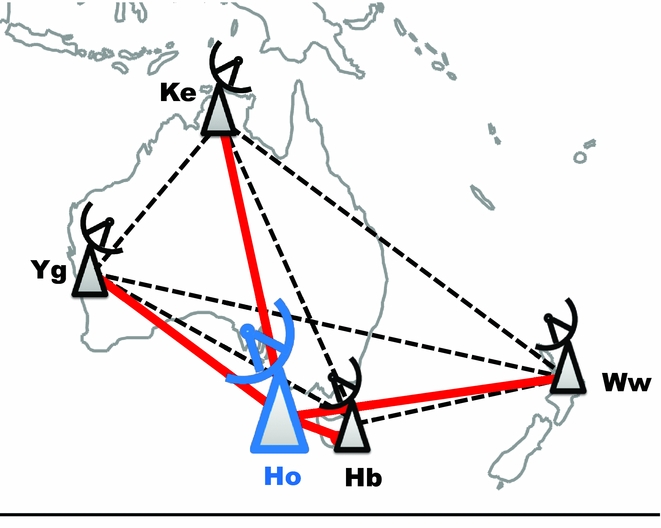
Figure 3. Illustration of the star mode. The scan length is determined only using the baselines including Ho (thick red lines).
In a standard AUSTRAL network, one has four stations (Hb, Ke, Ww, Yg) and six baselines (dashed lines). Since all four antennas are of similar type, they have similar sensitivities of ≈3600–4600 Jy in X-band and ≈4000–5200 Jy in S-band (Plank et al. Reference Plank2017). Using the standard AUSTRAL mode of 1 Gbps (Giga bit per second) recording, sources down to 0.4 Jy flux density can be observed with scan lengths of up to 500 s. Adding the Ho antenna (sensitivity of 1 200 Jy in X-band and 800 Jy in S-band) to the network shortens the scheduled observing time on the new baselines to Ho, while it does not change anything on the original baselines between the 12-m antennas.
The main feature of the star mode is that for a certain list of weak sources of interest, the scan length is only calculated for the baselines to Ho, ignoring the baselines between two 12-m antennas of lower sensitivity. This allows for observations of much weaker sources, in the case of the AUSTRAL array sources with flux densities down to about 0.15 Jy in X-band and 0.2 Jy in S-band. While without modification, these would yield scan lengths of 60 min or more, in the new mode scan lengths of maximum 10 min were scheduled. Examples for sessions scheduled with the star mode are presented in Section 2.4.
Since 2013, the Vienna VLBI Software (VieVS, Böhm et al. Reference Böhm, Böhm, Nilsson, Pany, Plank, Spicakova, Teke and Schuh2009) has been used for scheduling the AUSTRAL experiments. As first mentioned in Plank et al. (Reference Plank, Lovell, McCallum and Mayer2016), this software was amended for the star scheduling mode, as described step-by-step in the next Section (2.3). Since the 12-m telescopes are of similar sensitivities and relatively fast, they typically are scheduled together in the same scan with rapid slew times in between. This leads to many scans per hour (≈30–35) and improved geodetic results (see e.g. Plank et al. Reference Plank2017). By simply adding the slower Ho antenna to the network, the scheduling algorithm would favour larger networks. This in turn would lead to more idle time for the fast antennas, less scans per hour, and consequently a degradation of the geodetic results.
2.3. Scheduling algorithm
The implementation of the star scheduling mode into VieVS is shown in the flow chart of Figure 4.
Figure 4. Algorithm for the implementation of the star mode in VieVS.
In step 1, a list of target sources is defined. These are typically weak radio sources and their approximate flux densities in S- and X-band have to be known. In step 2, the sensitive antenna (Ho) has to be selected. Currently, the implementation was designed for one sensitive and slow antenna being added to a regional network of fast antennas of similar sensitivities. The scheduling itself works scan-by-scan (step 3). It is distinguished between every nth scan and all other scans. For all other scans (right branch in the flow chart), the special antenna (Ho) is removed from the core network. As described in more detail by Sun (Reference Sun2013), the stationwise scheduling algorithm in VieVS first collects all geometrically possible scans and subsequently weights them according to three selection criteria: each scan earns points for improving the sky coverage over each station, for a high number of observations and for a short scan duration. Typically, this process runs until the end of a session is reached. In the star mode, every nth scan deviates from the procedure above (left branch). Instead, the special antenna (Ho) is added to the network and a scan is formed with all stations to one of the target sources defined in step 1. Hereby, the programme cycles through the list of target sources. Also, in these scans, the scan duration is determined only considering the baselines including Ho. For the observed sessions, n was set to 10, which was identified as a good mixture between special scans and geodetic scans.
When the end of the session is reached, the schedule is first scanned for possible fill-in opportunities (step 4). These are additional scans that are added for the core network, when two or more antennas are idling while the others are still observing or slewing. The final step (5) is to identify scans of the core network which can be reached by the special antenna Ho in between the special scans. By adding Ho in so-called tag-along mode, it is guaranteed that the slower antenna does not degrade the geodetically optimised schedule and still increases its number of scans.
The star mode is a new feature of VieVS and was used to schedule four 24-h sessions in 2016.
2.4. Scheduled sessions
The new star scheduling mode was applied to four sessions in 2016 (Table 1). The data were correlated at the Shanghai Astronomical Observatory and fringe fitting was done at UTAS. All information about these experiments, including the schedules, correlated data, and analysis results, can be found via the master file website (http://lupus.gsfc.nasa.gov/sess/master16.html) of the IVS.
Table 1. Sessions scheduled with the new star mode. Each session lasted for 24 h and consisted of three or four 12-m antennas plus the Ho 26-m telescope.
The sessions’ network consisted of the AuScope 12-m antennas in Hb, Ke, and Yg plus Ww. In addition, the Ho 26-m telescope was added as the strong antenna. For the last two sessions, Hb could not observe due to maintenance work during that period.
Two source lists were used for scheduling, one comprising geodetically good and reasonably strong sources and additionally a list of 10–15 target sources per experiment. These target sources (Table 2) were selected from the ICRF2 catalogue, having a particularly low number of observations. Applying the star scheduling mode, we ended up with about 30 scans per hour for the 12-m antennas and 10–12 scans per hour for the Ho telescope. In the regular AUSTRALs, we find a maximum of 35 scans per hour for the 12-m telescopes. It has been shown (Plank et al. Reference Plank2017) that this improves the geodetic results in terms of baseline length repeatabilities compared to typically 10–15 scans per hour in the standard IVS experiments. We conclude that including observations of weak sources in the schedule does not significantly diminish the geodetic quality of the schedule measured by the number of scans for each station.
Table 2. List of target sources observed in aua009, aua010, aug024, and aug026. For each session, the statistics are given about the numbers of scheduled and successfully observed (i.e. correlated) observations. The percentages in columns five and six represent the ratio of successfully correlated observations as well as the percentage of observations that were found to be suitable to be included in the analysis. In the last four columns, the observed flux densities for X-band and S-band are shown together with their corresponding factors from the a priori values used in the scheduling.
3 RESULTS
Overall, the observed sessions were very successful. After analysis and geodetic estimation, a session fit between 33 and 43 ps was found. Despite four sessions being at the margin of statistical significance, baseline length repeatabilities were found to be between 2 and 5 mm for these sessions, indicating good geodetic results. More severe problems were found in aug026 as there are no data from Ww for half of the session due to bad weather. Ho was also intermittently stowed due to high winds, in total accumulating to about 6-h data loss.
In Table 2, the statistics of the observations to the target sources are shown.
In the third column, the number of scheduled observations is given. The target sources were scheduled for between 6 and 90 observations in a 24-h session. However, these cover the observations on all baselines, including the ones between the 12-m antennas. As these observations were not considered when determining the scan lengths, it is expected that they will have low SNR and subsequently are of less precision and not suitable for analysis. Studying Table 2, this is exactly what we find.
While from the originally scheduled observations most were successfully correlated (columns 4 and 5), the number of observations actually used is much lower. In column 6, the numbers of observations that were used in the analysis are given in percentages of the correlated observations. On average, 60% of the correlated observations were also used in the analysis. This means that sometimes also observations on the baselines between the 12-m antennas were used. The explanation for this is that in the scheduling when calculating the scan length the target SNRs are typically set much higher (20 or 15) than the SNR limit for a successful scan (typically 7). This is in order to account for changing source flux densities or other variables influencing the SNR during the observation (see e.g. Gipson & Baver Reference Gipson and Baver2016).
In the last four columns, the flux densities of the observed sources are given for X-band and S-band. They are estimated from the observed SNR for observations with a clear detection compared to the expected values derived from station sensitivities. The first number is the determined value, followed by the ratio of observed to expected flux density. One typically gets more useful observations when the source was assumed to be weaker (factors of >1) than it actually turned out to be and less observations when the factors are <1. These metrics do not include non-detections due to antenna-based problems such as wind stow. It shall also be noted that interference at S-band is particularly strong at Hobart which may be another reason why this relationship does not hold for every source. Overall, we obtained a good number of useful observations of all scheduled sources except one, 1334-649. Though this source has been detected in previous AUSTRAL experiments, it is possibly too weak to be properly observed with this network.
For some of the observed sources, these observations are the first flux density measurement for over 10 yrs. With the flux densities prone to significant variations over time (e.g. Shabala et al. Reference Shabala, Rogers, McCallum, Titov, Blanchard, Lovell and Watson2014), this is important for both determining an appropriate on source time in the scheduling as well as monitoring the sources’ astrophysical behaviour. For the more frequently observed sources, comparison of the flux densities of our sessions with the results of global IVS sessions showed good agreement.
Besides measurements of source flux densities, these sessions can also be used to accurately determine the positions of the observed sources. First, the observations were analysed sessionwise, using VieVS. For the estimation of source coordinates, the Earth orientation was fixed and standard settings were used for the other parameters (see e.g. Plank et al. Reference Plank2017). In Figure 5, the formal uncertainties in right ascension (RA) and declination (Dec) of the estimated source coordinates are given. Note that the standard geodetic and target sources have been plotted separately, with the latter ones typically having less observations and observed mainly on the star baselines only. This does affect the results. While the typical (median) uncertainties for the standard geodetic sources are 224 μas in RA and 276 μas in Dec, one finds higher uncertainties for the target sources, namely 391 μas in RA and 401 μas in Dec, respectively, in the single-session solution.
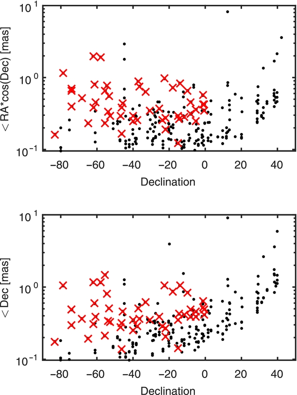
Figure 5. Formal uncertainties σ in right ascension (RA) and declination (Dec). As common, the former ones are scaled with cos(Dec). The sources were estimated in sessionwise solutions for aua009, aua010, aug024, and aug026. The target sources of Table 2 are marked with red crosses, while all other sources are represented by black dots. Note the logarithmic scale.
For final positions of the target sources, a global solution using the history of all VLBI observations since 1979 was calculated (Table 3). Comparing solutions with and without the four sessions described here, one finds significant improvements in the formal uncertainties for some of the target sources. As expected, the largest improvements were found for sources with initially having a very low number of observations. On average (mean over 42 sources), the four sessions improve the uncertainties in RA by 9% and in Dec by 12%.
Table 3. Positions of target sources observed in aua009, aua010, aug024, and aug026, computed at GSFC/NASA using Calc/Solve. A global solution was calculated using 6015 VLBI sessions from 1979 August 03 to 2016 July 13. Units of RA are hours, minutes, and seconds, units of Dec are degrees, minutes, and seconds. The uncertainties a σ are given in mas and σ RA are scaled with cos (Dec). In columns six and seven, the improvement in the uncertainties is shown, when calculating global solutions with the four new sessions compared to a solution without them. Finally, in the last two columns, the numbers of used observations per source are given for the first solution, as well as the additional observations added through the four new sessions.
a The formal errors in the table come directly from the GSFC solution and are likely too optimistic. A more realistic estimate would be obtained by applying a scale factor of 1.5 to the formal uncertainties followed by a root-sum-square increase of 40 μas of error in quadrature to the quoted values. This was the procedure adopted for ICRF2 (Fey et al. Reference Fey2015). That means the formal errors can be compared with each other but should not be compared with some other catalogues.
4 DISCUSSION
The star scheduling mode is a new feature of VieVS and has been successfully applied to four 24-h geodetic VLBI sessions, allowing us to determine the flux densities and positions of 42 target sources. While dropping several baselines will certainly badly affect the uv-coverage and subsequent imaging of the observed radio sources, the new mode does not harm the geodetic quality of the session. With the geodetic observing programme striving to increase the observations to a full 24-h on 7 d a week schedule (Nothnagel et al. Reference Nothnagel, Artz, Behrend and Malkin2016), this mode offers possibilities for other studies. For example, monitoring of changes in the flux densities can indicate astrophysical changes in the sources (Shabala et al. Reference Shabala, Rogers, McCallum, Titov, Blanchard, Lovell and Watson2014).
At the moment the mode was developed for the special case of the AUSTRAL network with the co-located Ho antenna, but it certainly can be applied in other networks. Possible amendments in the scheduling strategy then include a better inclusion of the star antenna into the regular schedule, as an alternative to the currently used tag-along option. For larger networks, a strategy for smart sub-netting should be developed. If a network has more than one antenna of significantly higher sensitivity, the scheduling algorithm needs to be further developed. Though the basic concept of the star mode, that only baselines to the more sensitive antennas are considered for calculating the scan duration would stay the same.
5 CONCLUSIONS
Since the advent of the AuScope VLBI array, its contribution to future improvement of the ICRF has been continually increasing through the observations of the AUSTRAL programme, alongside the classical IVS observations including the new antennas. Due to antenna limitations, the expected improvements are limited to relatively strong sources, with flux densities >0.6 Jy.
A new scheduling mode—the star mode—was introduced in this paper, which allows to include observations of weaker (≈0.2 Jy) radio sources when adding a single stronger radio telescope to the network. The new mode further maintains a high number of observations for the small and fast antennas in the network, which is important in a geodetically optimised schedule designed for measuring precise station coordinates.
The star scheduling mode now allows for the AuScope VLBI array and its AUSTRAL observing programme to take much more responsibilities in maintaining and improving the ICRF and further supporting special observing programmes for ICRF2-Gaia transfer sources or calibrator surveys for space-craft navigation.
Future amendments of this mode will allow it to be applied to other antenna networks, easing the efforts when scheduling inhomogeneous antenna capabilities when pairing the new fast and weak antennas with the slow and more sensitive legacy telescopes.
ACKNOWLEDGEMENTS
This study made use of data collected through the AuScope initiative, contracted through Geoscience Australia. AuScope Ltd is funded under the National Collaborative Research Infrastructure Strategy (NCRIS), an Australian Commonwealth Government Programme. The data correlation was performed at the Shanghai VLBI Correlator within the framework of the International VLBI Service for Geodesy and Astrometry (IVS). We are grateful to the IVS Data Centre at Goddard Space Flight Centre for maintaining statistics about all observations and providing regularly updated flux catalogues. This manuscript was reviewed by one anonymous reviewer, whose comments and suggestions are highly appreciated.
The authors thank the Austrian Science Fund (FWF) for supporting this work (project J 3699-N29 and SORTS I2204).


