


1. Introduction
Compound drops or double emulsions are special classes of drops composed of a core (or inner drop) encapsulated by a shell (or outer drop). Such combinatorial structures find a wide variety of applications, starting from industrial applications such as direct-contact heat exchange and materials processing (Morton, Subramanian & Balasubramaniam Reference Morton, Subramanian and Balasubramaniam1990; Sapei, Naqvi & Rousseau Reference Sapei, Naqvi and Rousseau2012) to biological applications like lipid-bilayer formation and recovery of leucocytes (Kan et al. Reference Kan, Udaykumar, Shyy and Tran-Son-Tay1998; Das, Mandal & Chakraborty Reference Das, Mandal and Chakraborty2020). Moreover, the outer protective shell of such a double emulsion makes it a preferred choice for controlled delivery of drugs, food additives and chemical reactants (Li et al. Reference Li2018; Liu et al. Reference Liu, Zhang, Fontana, Hirvonen and Santos2017; Muschiolik & Dickinson Reference Muschiolik and Dickinson2017; Thammanna Gurumurthy & Pushpavanam Reference Thammanna Gurumurthy and Pushpavanam2020). Such an ever-expanding canvas of applications has accordingly motivated intensified research in the arena of compound droplet generation (Loscertales et al. Reference Loscertales, Barrero, Guerrero, Cortijo, Marquez and Gañán-Calvo2002; Utada et al. Reference Utada, Lorenceau, Link, Kaplan, Stone and Weitz2005; Zhou, Yue & Feng Reference Zhou, Yue and Feng2006), as well as their dynamical manipulation including migration, breakup and coalescence (Chen, Liu & Shi Reference Chen, Liu and Shi2013; Kim & Dabiri Reference Kim and Dabiri2017; Borthakur, Biswas & Bandyopadhyay Reference Borthakur, Biswas and Bandyopadhyay2018), over the past two decades.
Drops are well known to be manipulatable via electric field mediated effects (Poddar et al. Reference Poddar, Mandal, Bandopadhyay and Chakraborty2019a; Vlahovska Reference Vlahovska2019; Wagoner et al. Reference Wagoner, Vlahovska, Harris and Basaran2020; Behera & Chakraborty Reference Behera and Chakraborty2023). Fundamentally, this stems from the establishment of electrical (Maxwell) stresses at the fluid–fluid interface owing to jump discontinuities in the respective electrophysical properties. Starting from the fundamental work of Taylor (Reference Taylor1966), numerous theoretical, experimental and application-oriented perspectives have subsequently been put forward on single-droplet electrohydrodynamics (Lac & Homsy Reference Lac and Homsy2007; Karyappa, Deshmukh & Thaokar Reference Karyappa, Deshmukh and Thaokar2014; Lanauze, Walker & Khair Reference Lanauze, Walker and Khair2015; Xi et al. Reference Xi, Guo, Leniart, Chong and Tan2016; Vlahovska Reference Vlahovska2019), resulting to the establishment of the knowhow of highly precise droplet manipulation and control.
In contrast to single-droplet electrohydrodynamics, studies reporting on the electrically manipulated dynamics of compound droplets have been relatively limited (Behjatian & Esmaeeli Reference Behjatian and Esmaeeli2013; Soni, Thaokar & Juvekar Reference Soni, Thaokar and Juvekar2018; Abbasi et al. Reference Abbasi, Song, Kim and Lee2019). This deficit in fundamental understanding may be attributed to the challenges in deciphering the strong coupling between the respective dynamics of the inner and outer drops as against considering them as isolated entities, bringing in additional geometry-mediated interactions that are by no means trivially tractable via established analytical theories, as aptly featured by early experiments and numerical simulations (Tsukada et al. Reference Tsukada, Mayama, Sato and Hozawa1997). Behjatian & Esmaeeli (Reference Behjatian and Esmaeeli2013) developed a closed-form analytical theory, albeit with certain restrictive assumptions, to explain the preferential occurrence of single or multiple compound droplets, depending on the relative tangential electrical stresses on the inner to outer drop. These findings were further advanced by studies on compound drop electrohydrodynamics under the combined effects of background flow and electric forcing, bringing out the relative role of the hydrodynamic and electrohydrodynmic stresses in dictating the drop migration and destabilization (Abbasi et al. Reference Abbasi, Song, Kim and Lee2019; Santra, Das & Chakraborty Reference Santra, Das and Chakraborty2020a; Santra et al. Reference Santra, Panigrahi, Das and Chakraborty2020b).
Despite the above advancements, the physical paradigms of electrically manipulated compound droplet dynamics have remained far from being well understood, primarily because of the restrictive assumption of either concentric drops (Soni, Juvekar & Naik Reference Soni, Juvekar and Naik2013; Behjatian & Esmaeeli Reference Behjatian and Esmaeeli2015; Abbasi et al. Reference Abbasi, Song, Kim and Lee2017; Su et al. Reference Su, Yu, Wang, Zhang and Liu2020) or only infinitesimal deviation from the same in the underlying theoretical propositions, which may deviate significantly from the physical reality (Gouz & Sadhal Reference Gouz and Sadhal1989; Boruah et al. Reference Boruah, Randive, Pati and Sahu2022). Such deviations from a concentric ideality essentially stem from the fact that, despite highly precise controls exercised during droplet generation, inevitable differences in the viscous drag acting at the two interfaces (Utada et al. Reference Utada, Lorenceau, Link, Kaplan, Stone and Weitz2005; Nabavi et al. Reference Nabavi, Vladisavljević, Gu and Ekanem2015;Yu et al. Reference Yu, Wu, Li and Liu2019), as well as property contrasts between the inner and the outer drops, may result in obvious deviations from concentricity. This, in turn, leads to simultaneous deformation and translation of the compound drop, as against the case of a concentric one that undergoes deformation without any net migration under a uniform external electric field (Baygents, Rivette & Stone Reference Baygents, Rivette and Stone1998; Das, Dalal & Tomar Reference Das, Dalal and Tomar2021; Sorgentone et al. Reference Sorgentone, Kach, Khair, Walker and Vlahovska2021). While the compelling need of rationalizing this deficit in theoretical understanding has been underpinned, the same remains far from being well resolved.
The fundamental origin of the discrepancy in rationalizing the electrically manipulated dynamics of eccentric compound drops based on concentric-drop theory lies in the fact that, despite uniformity in the applied external electric field, the asymmetries in the field lines due to the eccentric drop configuration lead to inhomogeneity in the inner-field distribution, giving rise to dielectrophoretic effects. This renders the situation conceptually analogous to single drops subjected to non-uniform electric fields (Thaokar Reference Thaokar2012; Mandal, Bandopadhyay & Chakraborty Reference Mandal, Bandopadhyay and Chakraborty2016a), resulting in an interplay of the electrohydrodynamic (EHD) and dielectrophoretic (DEP) forces, albeit with an additional complexity of being dynamically coupled with the spatio-temporal evolution of respective encapsulating entities as against a single drop in isolation. The EHD forces, well known to influence the dynamics of the individual droplet entities, essentially originate from the interfacial flow field that acts to balance a jump in the tangential electric stress (Taylor Reference Taylor1966), so as to ensure a continuity of the net local interfacial stress that stems from the cumulative electrical and hydrodynamic stresses. On the other hand, the DEP forces attribute fundamentally to the gradients in the local electric field, with no explicit contextual reference to fluid motion. While the EHD effects are commonly portrayed in the literature as playing a decisive role in the droplet migration under electrical forcing (Gouz & Sadhal Reference Gouz and Sadhal1989; Boruah et al. Reference Boruah, Randive, Pati and Sahu2022), there are, however, no rational premises of precluding a possible emphatic role of the DEP forces as well, typically when the electric field is likely to vary locally, despite its uniformity in the far stream. Further, the DEP effects likely to be inherently imperative for fluid pairs reminiscent of either perfect dielectrics or highly conducting entities suspended in a perfectly dielectric medium (Behjatian & Esmaeeli Reference Behjatian and Esmaeeli2013). However, no theoretical model has thus far been developed to bring out the underlying physics, whereas the standard EHD models for single droplets continue to be extended for explaining the electro-mechanics of compound droplets as well.
Here, we formulate an approximate analytical framework, assuming Stokes flow and negligible deformation limits, to delineate the role of DEP interactions in decisively manipulating the resulting morpho-dynamical evolution of an eccentric compound drop under uniform external electric field. Attributing the underlying physical features to a dynamically evolving eccentricity, we demonstrate the various possible combinations of the inner and the outer drop motion as functions of the pertinent electro-physical properties, eccentricity, and the radius ratio of the inner and the outer drops, based on an axisymmetric configuration. Our results decipher that, depending on these parameters, the relative velocity between the inner and outer drops may be directed alongside or opposite to the electric field direction, leading to four distinctive combinatorial migration characteristics. The results also implicate a non-monotonic trend in the relative velocity between the inner and outer drops with the variations in the eccentricity as well as the radius ratio, as attributed to a dynamic nonlinear coupling between the electrical and the hydrodynamic stresses. These central findings are likely to act as precursors towards the establishment of a design strategy for the active control of morphologically complex drops, cells and capsules in biological and engineered systems.
2. Theory
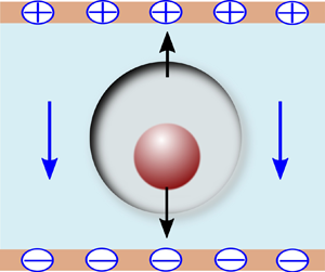
We consider an eccentric compound drop placed in a uniform electric field  $({\boldsymbol{E}_0} ={-} {E_0}{\kern 1pt} {e_z})$ inside an unbounded domain, as shown in figure 1(a). The inner drop (or core) of radius a and outer drop (or shell) of radius b have their centres located at $(0,0,{\tilde{z}_0} - \tilde{e})$ and $(0,0,{\tilde{z}_0})$, respectively, where $\tilde{e}$ is the dimensional distance between their centres and is defined as the eccentricity. The ratio between the drop radii is defined as k = a/b. The core, shell and external phases are denoted by 1, 2 and 3, respectively. All three phases are assumed to have equal density $\rho $, to nullify the buoyancy-driven effects and bring out the sole implications of the contrast of the electro-physical properties of the respective phases as the central focus of this work. The other material properties such as viscosity, electrical conductivity and electrical permittivity of the ith phase are symbolized by $\mu_i$, σi, and εi, respectively, where i = 1, 2 and 3. The ratios between the different physical properties of ith and jth fluid are defined as ${\lambda _{ij}}( = {\mu _i}/{\mu _j})$, ${R_{ij}}( = {\sigma _i}/{\sigma _j})$ and ${S_{ij}}( = {\varepsilon _i}/{\varepsilon _j})$, where i, j = 1, 2 and 3. These notations are in accordance with the previous works reported on related topics (Lac & Homsy Reference Lac and Homsy2007; Das & Saintillan Reference Das and Saintillan2017; Poddar et al. Reference Poddar, Mandal, Bandopadhyay and Chakraborty2019b; Sorgentone et al. Reference Sorgentone, Kach, Khair, Walker and Vlahovska2021; Behera & Chakraborty Reference Behera and Chakraborty2022) The surface tensions at the two interfaces are denoted as ${\gamma _{12}}$ and ${\gamma _{23}}$. Under the action of electric-field-induced forces, the inner and outer drops translate with velocities of ${U_1}$ and ${U_2}$, respectively, which are a priori unknown and are to be obtained from the model calculations.

Figure 1. (a) Schematic showing an unbounded eccentric compound drop placed in a uniform electric field  ${\boldsymbol{E}_0}$. The inner drop of radius a is placed inside a bigger drop of radius b at an off-centric position $(0,0,{\tilde{z}_0} - \tilde{e})$. (b) Geometric orientation of the compound drop in bispherical coordinate system $(\xi ,\eta ,\varPhi )$.
We normalize the model description by introducing the relevant scales consistent with the physics of the problem. Following previously reported studies (Behjatian & Esmaeeli Reference Behjatian and Esmaeeli2013; Santra et al. Reference Santra, Das and Chakraborty2020a; Boruah et al. Reference Boruah, Randive, Pati and Sahu2022), we use the radius of the outer drop, b, as a length scale, whereas the properties of the external medium are used to estimate the orders of magnitudes of the various stress components. The electric field and surface charge density are normalized with the magnitude of applied electric field E 0 and  ${\varepsilon _3}{E_0}$, respectively. The electric and viscous stresses are normalized by ${\varepsilon _3}E_0^2$ and ${\mu _3}{U_c}/b$, where ${U_c} = b{\varepsilon _3}E_0^2/{\mu _3}$ is the characteristic velocity scale, obtained by considering an interplay of these two stresses under the dynamic evolution of the physical system. The relative strengths between the electric stresses $({\varepsilon _3}E_0^2)$ and interfacial stresses (γ 12/a and γ 23/b) further dictate the extent of the drop deformation, as quantified by the respective electric capillary numbers: $C{a_{12}} = a{\varepsilon _3}E_0^2/{\gamma _{12}}$ and $C{a_{23}} = b{\varepsilon _3}E_0^2/{\gamma _{23}}$. Similarly, the ratio between the inertia and viscous stress is estimated by the hydrodynamic Reynolds number $Re = \rho {b^2}{\varepsilon _3}E_0^2/\mu _3^2$.
Whereas in principle an arbitrarily wide parametric space may be mathematically considered, we refer to the experiments of Tsukada et al. (Reference Tsukada, Mayama, Sato and Hozawa1997) for conforming to common practically realizable regimes. In their experiments, vegetable oil ( $\rho = 945\;\textrm{kg}\;{\textrm{m}^{ - 3}},\;\varepsilon = 38.05 \times {10^{ - 12}}\;\textrm{F}\;{\textrm{m}^{ - 1}}$, $\sigma = 1.68 \times {10^{ - 10}}\;\textrm{S}\;{\textrm{m}^{ - 1}},\;\mu = 0.254\;\textrm{Pa}\;\textrm{s}$) was used as the core and continuous phases, whereas silicone oil ( $\rho = 945\;\textrm{kg}\;{\textrm{m}^{ - 3}},\;\varepsilon = 22.1 \times {10^{ - 12}}\;\textrm{F}\;{\textrm{m}^{ - 1}}$, $\sigma = 2.67 \times {10^{ - 12}}\;\textrm{S}\;{\textrm{m}^{ - 1}}\textrm{,}\;\mu = 0.017\;\textrm{Pa}\;\textrm{s}$) was considered for the outer drop or shell phase. Similar oil phases are very common in a wide gamut of process engineering applications. The corresponding interfacial tension is around 3 mN m−1. Thus, for an applied external electric field of 20 kV m−1, and the inner and outer radii of 1 mm and 3 mm, respectively, we get: $C{a_{12}} \approx 0.005$, $C{a_{23}} \approx 0.015$ and $Re \approx 0.002$. In a more recent experimental study of Abbasi et al. (Reference Abbasi, Song, Kim and Lee2019), the core and the external medium were castor oil ( $\rho = 961\;\textrm{kg}\;{\textrm{m}^{ - 3}},\;\varepsilon = 41.6 \times {10^{ - 12}}\;\textrm{F}\;{\textrm{m}^{ - 1}},$, $\sigma = 3 \times {10^{ - 11}}\;\textrm{S}\;{\textrm{m}^{ - 1}},\;\mu = 0.78\;\textrm{Pa}\;\textrm{s}$), whereas silicone oil constituted the shell, having interfacial tension of 4.5 mN m−1. The castor oil–silicone oil pair exemplifies a common system used for studying the compound drop dynamics over experimentally tractable physical regimes (Santra et al. Reference Santra, Panigrahi, Das and Chakraborty2020b; Borthakur, Nath & Biswas Reference Borthakur, Nath and Biswas2021). For the ranges of experimental data traversed in Abbasi et al. (Reference Abbasi, Song, Kim and Lee2019), the above consideration leads to: $C{a_{12}} \approx 0.0037$, $C{a_{23}} \approx 0.011$ and $Re \approx 0.0002$. Irrespective of the wide variabilities in the physical data for these reported experimental studies, a common consensus is thus: $C{a_{12}},C{a_{23}} \ll 1$ and $Re \ll 1$. Physically, the same conforms to undeformed drops dynamically evolving under creeping flow conditions. Further note that the charge relaxation time scales for the above fluids, i.e. ${\varepsilon _1}/{\sigma _1}$ and ${\varepsilon _2}/{\sigma _2}$, are negligible compared with the fluid flow time scale ${\mu _3}/{\varepsilon _3}E_0^2$. Thus, the charging of the drops occurs much earlier than the flow development, so that the temporal regime of the dynamic distribution of the surface charge in effect becomes ‘instantaneous’.
2.1. Bispherical coordinates
We adopt a bispherical coordinate system (ξ, η, Φ), as depicted in figure 1(b), to gain theoretical insights into the electric field and fluid flow. The corresponding cylindrical coordinate system (r, z, Φ) may be described as (Happel & Brenner Reference Happel and Brenner1981; Poddar, Bandopadhyay & Chakraborty Reference Poddar, Bandopadhyay and Chakraborty2020, Reference Poddar, Bandopadhyay and Chakraborty2021)
 \begin{equation}r = \frac{{{c_0}\sin (\eta )}}{{\cosh (\xi ) - \cos (\eta )}},\quad z = \frac{{{c_0}\sinh (\xi )}}{{\cosh (\xi ) - \cos (\eta )}},\quad \varPhi = \varPhi .\end{equation}
The axes z = 0 and r = 0 are represented in the bispherical coordinates as  $\xi = 0$ and $\eta = 0\;\textrm{or}\;{\rm \pi}$, respectively. The inner and outer surfaces are denoted by $\xi = {\xi _{12}}$ and $\xi = {\xi _{23}}$, respectively, where ${\xi _{12}} > {\xi _{23}} > 0$. In (2.1), ${c_0}$ is a positive scaling factor, defined as ${c_0} = \sinh ({\xi _{23}}) = k\sinh ({\xi _{12}})$, where $k = a/b$ is the radius ratio. In figure 1(b), the dimensionless distances of the drop centres from the origin are ${z_1} = k\cosh ({\xi _{12}})$ and ${z_2} = \cosh ({\xi _{23}})$. Therefore, the dimensionless eccentricity is denoted as $e = |{z_1} - {z_2}|$. The coordinates of drop interfaces are related to eccentricity and radius ratio as
 \begin{equation}{\xi _{12}} = {\cosh ^{ - 1}}\left( {\frac{{1 - {e^2} - {k^2}}}{{2ek}}} \right),\quad {\xi _{23}} = {\cosh ^{ - 1}}\left( {\frac{{1 + {e^2} - {k^2}}}{{2e}}} \right),\quad k < 1 - e.\end{equation}
Accordingly, the z-coordinates of the drop centres can be obtained as
 \begin{equation}{z_1} = \frac{{1 - {e^2} - {k^2}}}{{2e}}\quad \textrm{and}\quad {z_2} = \frac{{1 + {e^2} - {k^2}}}{{2e}}.\end{equation}
It is to be noted that the limiting case of a concentric compound drop is recovered when  $e \to 0$, leading to ${\xi _{12}},\;{\xi _{23}},\;{z_1},\;{z_2} \to \infty$. With increase in e, the constituting drops would approach closer to the plane z = 0 or equivalently $\xi = 0$.
2.2. Governing equations and boundary conditions
2.2.1. Electrostatic problem
The subjection to the electric field causes drop polarization, leading to the accumulation of charges at the interface only (Melcher & Taylor Reference Melcher and Taylor1969; Saville Reference Saville1997). As per the leaky-dielectric model (Taylor Reference Taylor1966), the electric potentials of each charge-free bulk fluid satisfy the Laplace equation, which in bispherical coordinates reads (Moon & Spencer Reference Moon and Spencer1971)
 \begin{align}{\nabla
^2}{\varphi _i} &= \frac{{{{(\cosh \xi - \cos \eta
)}^3}}}{{c_0^2\sin \eta }}\left\{ {\frac{\partial
}{{\partial \xi }}\left( {\frac{{\sin \eta }}{{\cosh \xi -
\cos \eta }}\frac{{\partial {\varphi_i}}}{{\partial \xi }}}
\right)} \right.\nonumber\\
&\quad \left. { + \frac{\partial }{{\partial \eta
}}\left( {\frac{{\sin \eta }}{{\cosh \xi - \cos \eta
}}\frac{{\partial {\varphi_i}}}{{\partial \eta }}} \right)}
\right\} = 0;\quad i =
1,2,\textrm{3}\textrm{.}\end{align}
\begin{align}{\nabla
^2}{\varphi _i} &= \frac{{{{(\cosh \xi - \cos \eta
)}^3}}}{{c_0^2\sin \eta }}\left\{ {\frac{\partial
}{{\partial \xi }}\left( {\frac{{\sin \eta }}{{\cosh \xi -
\cos \eta }}\frac{{\partial {\varphi_i}}}{{\partial \xi }}}
\right)} \right.\nonumber\\
&\quad \left. { + \frac{\partial }{{\partial \eta
}}\left( {\frac{{\sin \eta }}{{\cosh \xi - \cos \eta
}}\frac{{\partial {\varphi_i}}}{{\partial \eta }}} \right)}
\right\} = 0;\quad i =
1,2,\textrm{3}\textrm{.}\end{align}
At the interface between the ith and jth phases, the surface charge density is calculated as  ${q_{S,ij}} = ({S_{i3}}\nabla {\varphi _i} - {S_{j3}}\nabla {\varphi _j})\boldsymbol{\cdot }{\boldsymbol{n}_{ij}}$. To obtain the final solution of ${\varphi _{1,2,3}}$, the following boundary conditions are further imposed: (i) the electric potential is bounded inside the inner drop, i.e. ${\varphi _1}$ is finite as $\xi \to \infty$; (ii) far away from the drop, the electric potential approaches the applied electric potential, i.e. ${\varphi _3} \to {\varphi _0} = z = {c_0}\sinh (\xi )/(\cosh (\xi ) - \cos (\eta ))$ as $\xi ,\eta \to 0$; (iii) at the interface between the ith and jth phases, the electric potentials satisfy continuity, i.e. ${\varphi _i} = {\varphi _j}\;\textrm{at}\;\xi = {\xi _{ij}}$; (iv) The interfacial charge evolution $\textrm{d}{q_S}/\textrm{d}t$ is governed by the ohmic conduction in the bulk fluids: $({\boldsymbol{J}_j} - {\boldsymbol{J}_i})\boldsymbol{\cdot }{\boldsymbol{n}_{ij}}$ (where Ji = Ri 3Ei is the ohmic current) and surface charge convection ${\nabla _{S,ij}}\boldsymbol{\cdot }({\boldsymbol{u}_{S,ij}}{q_{S,ij}})$ (where ${\nabla _S}$ is the surface gradient operator and ${\boldsymbol{u}_S}$ is the surface velocity). The charge conservation equation at the interface $\xi = {\xi _{ij}}$ takes the form
 \begin{equation}R{e_E}\left\{ {\frac{{\textrm{d}{q_{S,ij}}}}{{\textrm{d}t}} + {\nabla_S}\boldsymbol{\cdot }({\boldsymbol{u}_{S,ij}}{q_{S,ij}})} \right\} + ({\boldsymbol{J}_j} - {\boldsymbol{J}_i})\boldsymbol{\cdot }{\boldsymbol{n}_{ij}} = 0.\end{equation}
Here,  $R{e_E}( = \varepsilon _3^2E_0^2/({\sigma _3}{\mu _3}))$ is the electric Reynolds number that defines the ratio of the charge relaxation time $({\varepsilon _3}/{\sigma _3})$ and flow time scale $(b/{U_C})$. Under the assumption of a negligibly small charge relaxation time (i.e. the electrical Reynolds number $R{e_E} \ll 1$) justified earlier, the charge conservation equation at the interface $\xi = {\xi _{ij}}$ reduces to
 \begin{equation}({\boldsymbol{J}_j} - {\boldsymbol{J}_i})\boldsymbol{\cdot }{\boldsymbol{n}_{ij}} = 0.\end{equation}
The electric potential distribution, satisfying (2.4), is given as
 \begin{align}{\varphi
_i} &= {c_0}\sqrt {\cosh \xi - \cos \eta } \sum\limits_{n =
0}^\infty \{ {\alpha _{n,i}}\cosh (n + 1/2)\xi\nonumber\\
&\quad + {\beta _{n,i}}\sinh (n + 1/2)\xi \} {P_n}(\cos \eta );\quad i
= 1,2,3,\end{align}
\begin{align}{\varphi
_i} &= {c_0}\sqrt {\cosh \xi - \cos \eta } \sum\limits_{n =
0}^\infty \{ {\alpha _{n,i}}\cosh (n + 1/2)\xi\nonumber\\
&\quad + {\beta _{n,i}}\sinh (n + 1/2)\xi \} {P_n}(\cos \eta );\quad i
= 1,2,3,\end{align}where Pn is the nth-order Legendre polynomial and αn,i and βn,i are the unknown coefficients to be obtained using the electrostatic boundary conditions described above. The details of calculating the electric field components are provided in Appendix A. The expressions for the electric potentials for the bulk fluids and the electrostatic boundary conditions as expressed in bispherical coordinates are provided in Appendix B.
Using suitable recurrence relations of Pn in (B6) and (B8), and imposing the orthogonality conditions, one can obtain 6n linear algebraic equations from the electrostatic boundary conditions, which can be solved numerically to obtain the unknown coefficients (αn, 1, βn, 1, αn, 2, βn, 2, αn, 3, βn, 3). Although it is impracticable to consider the contributions of all spherical harmonics, a truncation of the series given (provided in (B3)–(B5) in Appendix B) up to a reasonably high value of n (say N) can be performed, by noting that the said coefficients decay in magnitude after a reasonably large N. The cutoff for N has been chosen such that the relative errors in these coefficients as well as in the values of  ${\varphi _i}$ between the (N + 1) and Nth terms remain less than 10−6, e.g. $|\{ \varphi _i^{(N + 1)} - \varphi _i^{(N)}\} /\varphi _i^{(N)}|< {10^{ - 6}}\textrm{ }$. We observed that the truncation limit N needs to be increased with the eccentricity (e) and radius ratio (k) to retain the same numerical accuracy. A similar observation was reported by Jadhav & Ghosh (Reference Jadhav and Ghosh2021) in the context of a different physical problem of thermo-capillary migration. We verified that, for k = 0.1, the limit N = 20 can produce accurate results for eccentricities e ≤ 0.5. Since the information of the compound drop geometry (e, k) is provided to the theoretical model through the coordinate ξ 23 or ξ 12 (refer to (2.2)), instead of identifying the upper limits of (e, k), we identified the equivalent lower limits of ξ 23 up to which N = 20 can ensure series convergence. (refer to Appendix C).
Now, the electric traction forces exerted by the ith phase can be evaluated as
 \begin{equation}{\boldsymbol{T}_{E,i}} = {\boldsymbol{\tau }_{E,i}}\boldsymbol{\cdot }{\boldsymbol{n}_{ij}} ={-} {S_{i3}}\frac{{E_{\xi ,i}^2 - E_{\eta ,i}^2}}{2}{\boldsymbol{e}_\xi } - {S_{i3}}{E_{\xi ,i}}{E_{\eta ,i}}{\boldsymbol{e}_\eta }.\end{equation}
While the electric tractions combinatorically compel the drop to migrate, the axial component of the corresponding driving force is of particular interest for the focus of the present work because of its explicit contribution to the DEP motion. The total DEP force acting on the inner and outer drops can be calculated by integrating the axial traction acting on an elementary surface area, dS, as (Mandal et al. Reference Mandal, Bandopadhyay and Chakraborty2016a)
 \begin{align}{F_{DEP,1}} &= \int_S {({\boldsymbol{T}_{E,2}} \cdot {\boldsymbol{e}_z})\,\textrm{d}{S_{12}}} = \int_0^{2\mathrm{\pi }} {\int_0^\mathrm{\pi } {({\boldsymbol{T}_{E,2}} \cdot {\boldsymbol{e}_z})} } \frac{{c_0^2\sin \eta }}{{{{(\cosh {\xi _{12}} - \cos \eta )}^2}}}\,\textrm{d}\eta \,\textrm{d}\varPhi ,\end{align}
 \begin{align}{F_{\,DEP,2}} &= \int_S {({\boldsymbol{T}_{E,3}}\boldsymbol{\cdot }{\boldsymbol{e}_z})\,\textrm{d}{S_{23}}} = \int_0^{2\mathrm{\pi }} {\int_0^\mathrm{\pi } {({\boldsymbol{T}_{E,3}}\boldsymbol{\cdot }{\boldsymbol{e}_z})} } \frac{{c_0^2\sin \eta }}{{{{(\cosh {\xi _{23}} - \cos \eta )}^2}}}\,\textrm{d}\eta \,\textrm{d}\varPhi, \end{align}
The tangential component of the electric traction  ${\tau _{\xi \eta ,i}}( = {\boldsymbol{T}_{E,i}}\boldsymbol{\cdot }{\boldsymbol{e}_\eta })$ induces a non-uniform flow field in the drop vicinity, which exerts the electrohydrodynamic force $({F_{EHD}})$ on the inner and outer drops. Evaluation of ${F_{EHD}}$, thus, necessitates the solution of the flow field, as described subsequently.
2.2.2. Flow problem
For Stokes flow, the momentum and continuity equations are expressed as
 \begin{equation}{\lambda _{i3}}{\nabla ^2}{\boldsymbol{u}_i} = \boldsymbol{\nabla }{p_i},\quad \boldsymbol{\nabla }\boldsymbol{\cdot }{\boldsymbol{u}_i} = 0;\quad i = 1,2,3,\end{equation}
where u and p stand for velocity and pressure field, respectively. Here, the sole driving force for the fluid flow, i.e. the external electric field, acts along the z-axis. In the absence of any source of asymmetry about the same axis, (2.11) can be transformed into
 \begin{equation}{\varOmega ^2}({\varOmega ^2}{\psi _i}) = 0;\quad i = 1,2,3.\end{equation}
Here,  $\psi (\xi ,\eta )$ is the streamfunction, and ${\varOmega ^2}$ is a linear operator of the form
 \begin{equation}{\varOmega ^2} = \frac{{\cosh \xi - \zeta }}{{c_0^2}}\left\{ {\frac{\partial }{{\partial \xi }}\left( {(\cosh \xi - \zeta )\frac{\partial }{{\partial \xi }}} \right) + (1 - {\zeta^2})\frac{\partial }{{\partial \zeta }}\left( {(\cosh \xi - \zeta )\frac{\partial }{{\partial \zeta }}} \right)} \right\},\end{equation}
where  $\zeta = \cos (\eta )$. Like the electric potential, the velocity field satisfies the boundedness in the inner drop, i.e. ${\boldsymbol{u}_1}$ is finite as $\xi \to \infty$. Notably, the velocity fields of all the phases are redefined with respect to the reference frame adhering to the outer drop. Thus, the velocity at the far field, i.e. at $\xi \to 0$, $\eta \to 0$, is uniform and is obtained as $- {U_2}{e_z}$. In addition, at the interfaces, the tangential velocities are continuous, i.e. ${\boldsymbol{u}_i}\boldsymbol{\cdot }{\boldsymbol{t}_{ij}} = {\boldsymbol{u}_j}\boldsymbol{\cdot }{\boldsymbol{t}_{ij}}$ at ξ = ξij, and the normal velocity components satisfy the no-penetration boundary condition
 \begin{equation}\left. {\begin{array}{@{}c@{}} {{\boldsymbol{u}_2}\boldsymbol{\cdot }{\boldsymbol{n}_{23}} = {\boldsymbol{u}_3}\boldsymbol{\cdot }{\boldsymbol{n}_{23}} = 0\;\textrm{at}\;\xi \textrm{ = }{\xi_{23}}\textrm{ }}\\ {{\boldsymbol{u}_1}\boldsymbol{\cdot }{\boldsymbol{n}_{12}} = {\boldsymbol{u}_2}\boldsymbol{\cdot }{\boldsymbol{n}_{12}} = ({U_1} - {U_2}){\boldsymbol{e}_z}\boldsymbol{\cdot }{\boldsymbol{e}_\xi }\;\textrm{at}\;\xi \textrm{ = }{\xi_{12}}} \end{array}} \right\}.\end{equation}
The interfacial tangential stress balance concerns the combined electrical and hydrodynamic stresses, so that
 \begin{equation}{[\tau _{\xi \eta }^E]_{ij}} + {[\tau _{\xi \eta }^H]_{ij}} = 0,\end{equation}
where  $\tau _{\xi \eta }^E = {\boldsymbol{t}_{ij}}\boldsymbol{\cdot }({\tau ^E}\boldsymbol{\cdot }{\boldsymbol{n}_{ij}})$ and $\tau _{\xi \eta }^H = {\boldsymbol{t}_{ij}}\boldsymbol{\cdot }({\tau ^H}\boldsymbol{\cdot }{\boldsymbol{n}_{ij}})$ denote the tangential electric and hydrodynamic stresses, respectively, and [ ]ij represents the jump in the physical quantities at the interface $\xi \textrm{ = }{\xi _{ij}}$. The expressions of the electric stress tensor $({\tau _E})$ and the hydrodynamic stress tensor $({\tau _H})$ associated with ith phase, considering the individual phases to be homogeneous, isotropic and Newtonian are as follows:
 \begin{equation}\boldsymbol{\tau }_i^E = {S_{i3}}\{ {\boldsymbol{E}_i}{\boldsymbol{E}_i} - E_i^2\boldsymbol{I}\} ,\quad \boldsymbol{\tau }_i^H ={-} {p_i}\boldsymbol{I} + {\lambda _{i3}}\{ \boldsymbol{\nabla }{\boldsymbol{u}_i} + {(\boldsymbol{\nabla }{\boldsymbol{u}_i})^\textrm{T}}\} .\end{equation}
The general solution to the axisymmetric streamfunctions satisfying the biharmonic equation given in (2.12) is as follows:
 \begin{equation}{\psi _i} = {(\cosh \xi - \cos \eta )^{ - 3/2}}\sum\limits_{n = 0}^\infty {{W_{n,i}}} (\xi )C_n^{ - (1/2)}(\cos \eta ),\quad i = 1,2,3,\end{equation}
where  ${W_{n,i}}(\xi ) = {A_{n,i}}\,{\textrm{e}^{ - (n - 1/2)\xi }} + {B_{n,i}}\,{\textrm{e}^{(n - 1/2)\xi }} + {C_{n,i}}\,{\textrm{e}^{ - (n + 3/2)\xi }} + {D_{n,i}}\,{\textrm{e}^{(n + 3/2)\xi }}$ and $C_{n + 1}^{ - 1/2}$ is the Gegenbauer polynomial. Details regarding the application of different flow boundary conditions and the expressions of the tangential stresses are provided in Appendix B. Applying the useful identities (provided in Appendix D) to the boundary conditions gives us a set of algebraic equations which can be solved to obtain the unknown coefficients An ,1, Bn ,1, Cn ,1, Dn ,1, …, etc. Similar to the electrostatic problem, we have truncated the series of ψ after 20 terms without compromising the accuracy of the solutions. It is verified that in the pertinent limiting conditions (i.e. $e \to 0$), our approximate analytical solutions converge well with the previously reported closed form analytical solutions of Behjatian & Esmaeeli (Reference Behjatian and Esmaeeli2013) (refer to Appendix E).
One apparently paradoxical observation that appears to be evident from the expression of the flow field is that it does not include the surface tension. While this might lead to an inference that the surface tension is neglected in the balance of forces, it may be rationalized by noting that the dynamic surface tension force depends on the extent of deformation of the fluid–fluid interfaces. In the asymptotic theory, the interfacial deformation is rendered inconsequential at the leading order, bearing no influence on the mathematical representation of the normal force balance. Further, in the absence of any Marangoni effect (stemming from possible thermal or concentration gradients that are absent in the present set-up), there is no contribution of surface tension on the tangential stress balance either. Therefore, the overall stress balance depends on the hydrodynamic and the Maxwell stresses alone, with no role for the surface tension mediated interactions in dictating the dynamical evolution of the drop as per the asymptotic theory.
The essential foundations of the asymptotic theory, elucidated above, bring in obvious limitations of the same in capturing both qualitative and quantitative features of the droplet morpho-dynamics beyond a set of restrictive considerations. While these aspects of simplifications in the hydrodynamic model have previously been discussed in the context of the asymptotic analysis, we outline here some of the concerned inadequacies of the coupled electro-mechanical model. For instance, the expression for the outer electric potential  ${\varphi _3}$, can be written in the form: ${\varphi _3} = {\varphi _0} + {\varphi _{3,per}} = z + {\varphi _{3,per}}$, where ${\varphi _0}$ is the unperturbed far-field potential and ${\varphi _{3,per}}$ is the perturbation in the outer electric potential, generated due to the presence of the drop. Looking at the general solution of ${\varphi _3}$ (refer to (B5)), it can be well comprehended that ${\varphi _{3,per}}$ decays with a decrease in ξ and finally comes down to zero at ξ = 0. Accordingly, at the horizontal plane z = 0 (where ξ = 0), the outer electric potential takes the value ${\varphi _3} = z = 0$. This theoretical premise mimics the physical reality quite aptly for small values of the eccentricity because, in these cases, the plane z = 0 (or the fixed potential line) remains far away from the drop, thereby facilitating an asymptotic decay of the imposed perturbations. However, with increase in e, the drop's initial position gets closer to the fixed potential line. This may impact the accuracy of the solution adversely, since the perturbations are to be artificially quenched within a short distance. This results in inevitable inaccuracies in the semi-analytical solution that may best be circumvented by full-scale numerical simulations. We, therefore, perform numerical simulations in parallel to figure out a threshold limit of eccentricity up to which the semi-analytical and the numerical simulations agree, as described in § 3.4. Notably, the small eccentricity limit for the validity of the semi-analytical solution is pertinent only for the electrostatic problem and not for the hydrodynamic problem. The latter becomes the case since z = 0 does not conform to a hydrodynamic confinement, so that the hydrodynamic aspects remain akin to unbounded flows (Gouz & Sadhal Reference Gouz and Sadhal1989; Mandal, Ghosh & Chakraborty Reference Mandal, Ghosh and Chakraborty2016c; Jadhav & Ghosh Reference Jadhav and Ghosh2021; Boruah et al. Reference Boruah, Randive, Pati and Sahu2022).
2.2.3. Evaluation of drop migration velocities
The unknown drop velocities can be obtained by applying the dynamic force balance  $\sum F = {F_{DEP}} + {F_H} = \textrm{0}$ to each drop. Here, FH is the total hydrodynamic force, which is the summation of the viscous drag force Fdrag (due to the translation of the drop with respect to a background fluid medium) and the EHD force ${F_{EHD}}$. The latter originates from the EHD circulations that set in to satisfy the tangential force balance at the interface, which requires the consideration of both the hydrodynamic and the electrical (Maxwell) stress for its rationalization. While ${F_{DEP}}$ on the droplets can be calculated using (2.9) and (2.10), the dimensionless total hydrodynamic force (FH) acting on the droplets can be expressed as (Mandal et al. Reference Mandal, Ghosh and Chakraborty2016c)
 \begin{equation}{F_{H,1}} = \frac{{4\sqrt 2 \mathrm{\pi }}}{{{c_0}}}\sum\limits_{n = 0}^N {({B_{n,2}} + {D_{n,2}})} ,\quad {F_{H,2}} = \frac{{4\sqrt 2 \mathrm{\pi }}}{{{c_0}}}\sum\limits_{n = 0}^N {({B_{n,3}} + {D_{n,3}})} .\end{equation}
Note that the velocity coefficients (Bn ,2, Dn ,2, Bn ,3, Dn ,3) are linear functions of U 2 and U 1, obtained as  ${B_{n,2}} = K_{n,2}^{(B)}{U_1} + L_{n,2}^{(B)}{U_2} + M_{n,2}^{(B)}$, ${D_{n,1}} = K_{n,2}^{(D)}{U_1} + L_{n,2}^{(D)}{U_2} + M_{n,2}^{(D)}$ and so on, where $K_{n,2}^{(B)},L_{n,2}^{(B)}, \ldots M_{n,3}^{(B)}$ are functions of $({\xi _{12}},{\xi _{23}},{R_{23}},{R_{12}},{S_{23}},{S_{12}},{\lambda _{23}},{\lambda _{12}},n)$. Therefore, the force balance conditions can be transformed to
 \begin{align}&{U_1}\sum\limits_{n = 0}^N {(K_{n,2}^{(B)} + K_{n,2}^{(D)})} + {U_2}\sum\limits_{n = 0}^N {(L_{n,2}^{(B)} + L_{n,2}^{(D)})} + \sum\limits_{n = 0}^N {(M_{n,2}^{(B)} + M_{n,2}^{(D)})} + \frac{{{c_0}{F_{DEP,1}}}}{{4\mathrm{\pi }\sqrt 2 }} = 0,\end{align}
 \begin{align}&{U_1}\sum\limits_{n = 0}^N {(K_{n,3}^{(B)} + K_{n,3}^{(D)})} + {U_2}\sum\limits_{n = 0}^N {(L_{n,3}^{(B)} + L_{n,3}^{(D)})} + \sum\limits_{n = 0}^N {(M_{n,3}^{(B)} + M_{n,3}^{(D)})} + \frac{{{c_0}{F_{DEP,2}}}}{{4\mathrm{\pi }\sqrt 2 }} = 0,\end{align}
which are solved to obtain the drop velocities.
The temporal evolution of e can be defined as  $\textrm{d}e/\textrm{d}t = {U_2} - {U_1} = \varDelta U$ (where $\varDelta U$ is the relative velocity), which is inherently nonlinear because U 1 and U 2 are themselves functions of e. The eccentricity as a function of time is obtained using a numerical integration technique. For this purpose, we employ the ODE45 solver in MATLAB as an established means of implementing the Runge–Kutta method (Shampine & Reichelt Reference Shampine and Reichelt1997). This specific solver is robust since it can adaptively vary the time steps to ensure the required relative tolerance is achieved (10−8 in this case) by employing a six-stage fifth-order variant of the Runge–Kutta scheme. The initial condition used here is e(t = 0) = e 0.
3. Results and discussion
In this section, we focus on the key aspects of the droplet migration characteristics as influenced by the eccentricity-induced dielectrophoresis. We demonstrate the variation in results with a wide range of dimensionless electro-physical parameters (R 12, S 12, R 23 and S 23) and configurational variables (e and k). A plausible electro-physical parametric regime can be identified using the properties of vegetable oil, silicone oil and castor oil given in § 2, and by choosing their different combinations as the constituents of the inner drop, outer drop and the carrier phases, respectively. Considering the properties of the above-mentioned fluids, we calculate that the electrical permittivity ratios S 12,  ${S_{23}}\sim O(1)$ and R 12, R 23 to vary between O(10−2) and O(102). From an experimental perspective, different ranges of electro-physical parameters, even beyond the ones described above, can be readily achieved by using the doping technique (Yin & Zhao Reference Yin and Zhao2002), rendering practicable our parametric sweeps over the regimes explored.
Considering that the electric field is the sole driving force for drop motion, we first illustrate the comparison between the electric field distribution around the concentric and eccentric compound drops in figures 2(a) and 2(b), respectively, for R 23 = 0.01, S 23 = 5, R 12 = 0.01 and S 12 = 0.5, in an effort to bring out the exclusive role of the geometric eccentricity. As shown in this figure, the electric field (E) is symmetrically distributed about the equator for a concentric case, i.e. when  $e \to 0$. In the case of e = 0.25, the off-centric positioning of the inner drop towards the polar location η = π causes large perturbations in the local electric field, whereas the perturbations due to the inner drop's existence at the other polar point (at the outer surface of the shell) become less. Consequently, the electric field becomes asymmetric about the equatorial lines of each drop. This deviation from symmetry significantly impacts the electric as well as the hydrodynamic tractions manifested through the interfacial stress balance conditions (refer to (B14)). The intriguing migration characteristics of the drops attributable to the forces, originating from the respective tractions, are explained in detail in the subsequent sections.

Figure 2. Contour plot showing the magnitude of electric field |E| in the region close to the drop for (a) concentric and (b) eccentric compound drop cases for radius ratio k = 0.333. The electrical properties considered are R 23 = 0.01, S 23 = 5, R 12 = 0.01 and S 12 = 0.5. In (a) z 1,  ${z_2} \gg 1$ as $e \ll 1$ (refer to (2.3)).
3.1. Role of DEP force on drop migration
Figures 3(a) and 3(b) depict the effect of eccentricity, e, on the axial components of electric tractions over the interface of the drops. The geometric and electrical parameters are same as that chosen for figure 2. In figure 3, θ 1 and θ 2 represent the angular locations on the inner and outer interfaces, respectively (described in the insets). As shown, for e = 0.001 (nearly concentric case), the axial tractions acting on both the drops are anti-symmetric about the equator. Therefore, the net DEP force acting on the drops becomes zero. On the other hand, for e = 0.25, the axial tractions are conspicuously asymmetric. Although the off-centric positioning leads to a decrease in tractions on both sides of the equator, in the southern half, i.e. θ = π/2 to π, the alterations are comparatively high. Accordingly, the total axial forces acting on the southern half of the drops (which is positive) are relatively lower than their other half (which is negative), encouraging the movement of the drops in the negative z-direction. Note that the electric field, and hence the nature of the tractions, largely depends on the electric properties and geometric parameters. Therefore, multiple migration possibilities can be seen, as discussed next.

Figure 3. Effect of eccentricity (e) on the distribution of axial electric traction at the (a) inner surface, and (b) outer surface. The parameters considered are R 23 = 0.01, S 23 = 5, R 12 = 0.01 and S 12 = 0.5.
The EHD circulations and the concerned forces do not come into play if we disregard the tangential electric stress that drives the EHD circulations in the system, i.e.  $\boldsymbol{\tau }_{\xi \eta ,2}^E = \boldsymbol{\tau }_{\xi \eta ,1}^E = 0$. This mathematical consideration allows us to analyse the sole effects of the DEP forces. Physically, the absence of EHD circulations is possible only if the system is comprised of non-conducting (or perfectly dielectric) fluids. As the perfectly dielectric fluids do not develop charges on the surface, i.e. ${q_S} = 0$, the solutions to such fluid systems can be obtained by setting R 23 = S 23 and R 12 = S 12 (Melcher & Taylor Reference Melcher and Taylor1969). It is to be noted that the present analysis does not entirely stand for the dielectric system (as R 12 and R 23 are subjected to variations keeping S 12 and S 23 constants); however, the above mathematical consideration helps us to uncover the underlying physics dictating the translational dynamics of the compound drop system of concern here.
From the definitions of the DEP forces (refer to (2.8)–(2.10)), it can be inferred that in a functional form  ${F_{DEP}} = f({R_{23}},{R_{12}},{S_{23}},{S_{12}},e)$. Accordingly, in figures 4(a) and 4(b), we depict the effect of R 23 on the velocity of inner (U 1) and outer droplet (U 2), respectively, for different R 12. The conductivity ratio R 23 is varied between ${10^{ - 2}}$ and 102. It is observed that both U 1 and U 2 vary non-monotonically with R 23 as well as R 12. The transition in the trend in the velocity variation occurs at R 23 = 1 for all cases, and therefore, is named as the critical point. For R 12 = 1, the sign of U 1 and U 2 remains negative for all R 23. On the other hand, for R 12 = 0.01 and 100, U 1 changes its sign at R 23 = 1, while the sign of U 2 remains unaltered. For the latter two values of R 12, as R 23 is raised above unity, U 1 continuously increases until specific values of R 23 are reached, hereinafter named as the secondary critical values of R 23. Beyond these critical points, we observe a decreasing trend in U 1. Notably, for R 12 = 100, this secondary critical value of R 23 is greater than that of R 12 = 0.01. With a further increase in R 23, the U 1 versus R 23 curves for different R 12 begin to converge, ultimately following the same increasing (in magnitude) trend. However, R 23 = 1 acts as the point of convergence as far as the outer drop velocity U 2 is concerned.

Figure 4. Variations in (a) inner drop velocity U 1, (b) outer drop velocity U 2 and (c) DEP forces (FDEP ,1, FDEP ,2) with R 23 for different R 12. The other system properties are S 23 = 5, S 12 = 0.5, e = 0.15, k = 0.333 and z 2 = 3.04.
The contrasting set of drop characteristics presented in figures 4(a) and 4(b) can be explained by analysing the DEP force acting on the inner and outer drops, as portrayed in figure 4(c). It is noteworthy that the DEP force acting on the outer drop, FDEP ,2, while considerably varying with R 23, alters negligibly with variation in R 12. Some qualitative insights of the same may be put in perspective by appealing to the previously reported analytical theory on the electrically modulated dynamics of concentric compound drops (Behjatian & Esmaeeli Reference Behjatian and Esmaeeli2013, Reference Behjatian and Esmaeeli2015). Their analysis clearly reveals that the outer electric field has a strong dependence on R 23. In contrast, a significantly weak dependence on R 12 and the size ratio k was reported. However, the electric field inside the shell (or outer drop) strongly depends on R 23, R 12 and k, which is aptly evidenced from the variations of FDEP ,1 as shown in figure 4(c) herein. Depending on the nature of the DEP forces, three distinct regimes can be identified, i.e. regimes I, II and III. In regime I, which is typically restricted up to R 23 = 1, the forces on the inner and outer drop act on the negative z-direction. However, over this regime, as |FDEP ,1| > |FDEP ,2|, faster movement of the inner drop than the outer one occurs. Contrarily, over regime II, FDEP ,1 is positive, but FDEP ,2 is negative.
Despite the overwhelming importance of the DEP forces on the dynamics of the eccentric compound drops, their motions are further hindered by the viscous drag forces that are by themselves proportional to U 2,DEP, and U 1,DEP which are the DEP velocities of the outer and inner drop, respectively. Over regime I, as FDEP ,1, FDEP ,2 < 0, the drops move in the negative z-direction irrespective of the magnitude of the viscous drag. However, in regime II, the viscous drag causes some non-trivial alterations in the drop migration. Even though the signs of the DEP forces (FDEP ,1 > 0 and FDEP ,2 < 0) intuitively suggest that U 1 > 0 and U 2 < 0, respectively, throughout regime II, a sign reversal of U 1 occurs in practice, as delineated earlier. This is because of the fact that, beyond a critical point,  $|{F_{DEP,1}}|\gg |{F_{DEP,2}}|$, causing a much faster movement of the outer drop as compared with the inner one. For the considered parametric space, as the viscous drag acting on the inner drop is stronger than FDEP, 1, sign reversal in U 1 occurs. The reason behind the rapid weakening of FDEP, 1 for R 23 > 1 is that, at the outer boundary, the electric fields satisfy ${\boldsymbol{E}_2}\boldsymbol{\cdot }\boldsymbol{n} = ({\boldsymbol{E}_3}\boldsymbol{\cdot }\boldsymbol{n})/{R_{23}}$ (refer to (2.6)). Thus, an increase in R 23 produces a weaker electric field inside the outer drop (or shell) compared with the external medium, thereby resulting in a relatively weaker DEP force on the inner drop. Over regime III, where ${R_{23}} \gg 1$, the electric field inside the outer drop becomes negligibly small, i.e. ${F_{DEP,1}} \to 0$. However, the force on the outer and, therefore, the viscous drag remains significantly high. This forces the inner drop to migrate along with the outer one in the negative z-direction.
We further probe regime II in an effort to delve deeper into its non-trivial dynamic characteristics mentioned above, for various geometric orientations considering R 12 = 0.01 and R 23 = 1.5, keeping the other electro-physical properties unchanged. Figure 5(a) depicts the effect of the eccentricity of the compound drop configuration on the velocity variations, for different size ratios (k). It is observed that, when k is small, e.g. k = 0.2, the migration velocities of the slightly eccentric drops (i.e.  $e \ll 1$) are negligibly small (O (10−6)). Under such conditions, an increase in the eccentricity results in noticeably faster movements of the inner and outer drops in the negative z-direction, i.e. U 1, U 2 < 0. For higher values of k, although |U 1| and |U 2| vary in a similar manner with e, their directions may alter preferentially. For k = 0.333, for instance, U 1 > 0, and U 2 < 0, whereas for k = 0.55, U 1, U 2 > 0.

Figure 5. Effect of eccentricity e on the (a) velocities of inner and outer drops, and (b) DEP forces acting on the inner and outer drop. The other considered parameters are R 23 = 1.5, S 23 = 5, R 12 = 0.01, S 12 = 0.5 and k = 0.333 (which corresponds to the regime II). The lowest vertical height of outer drop centre (z 2) considered here is 1.52.
To explain the above counterintuitive features, we study the effect of the geometric parameters on the nature of the DEP forces, which is presented in figure 5(b). As shown in this figure, irrespective of considered geometric parameters, FDEP ,1 > 0 and FDEP ,2 < 0. An increase in e enhances the non-uniformity in the tractions, causing increments in FDEP ,1 and FDEP ,2. Conversely, when k is increased, FDEP ,1 increases significantly, whereas FDEP ,2 varies inconsequentially with k. From the expressions of the total DEP forces given in (2.9) and (2.10), it can be inferred that an increase in k leads to a large increment in the surface area of the inner drop  $({\propto} {k^2})$ only. Accordingly, only the inner drop senses large augmentation in the DEP force. On the other hand, the surface area of the outer drop remains unaltered, and thus, FDEP ,2 remains effectively unchanged. For k = 0.2, since $\textrm{|}{F_{DEP,1}}\textrm{|} \ll |{F_{DEP,2}}|$, the flow as triggered by the outer drop's motion is strong enough to overcome the drag produced by FDEP ,1 on the inner one. Therefore, the inner and outer drops move in the same (-z) direction. On the contrary, for k = 0.55, $\textrm{|}{F_{DEP,1}}\textrm{|} \gg |{F_{DEP,2}}|$, resulting in their migrations in opposite directions. For intermediate values of k, for example, for k = 0.333, as $\textrm{|}{F_{DEP,1}}\textrm{|} \approx |{F_{DEP,2}}|$ for each e, the drops are driven in the direction of the respective DEP forces acting on them.
3.2. Combined effect of DEP force and EHD force on the drop migration
Here, we consider both EHD and DEP forces, going beyond the limiting conditions considered in the preceding section. The translational behaviours of the drops are summarized as regime plots in R 12–R 23 space in figures 6(a) and 6(b) for (S 23, S 12) = (5, 0.5) and (S 23, S 12) = (0.5, 5), respectively. Depending on the directions of their movements, three major regimes have been identified, namely regimes A, B and C. For the conductivity ratios within regime A, the inner and the outer drops exhibit motion in the negative z-direction, i.e. U 1, U 2 < 0. On the other hand, regimes B and C are characterized by opposite movements of the drops, i.e. (U 1 > 0, U 2 < 0) and (U 1 < 0, U 2 > 0), respectively. In addition, regime A is discontinuously spanned as a fraction of it is limited up to R 23 ∼ 10, R 12 ∼ 1, whereas the other part of the same regime is encountered when  ${R_{23}} > 25({\gg} 1)$. Regime B is a sandwiched zone between the two halves of regime A. In contrast, regime C can be located towards the increasing R 12 direction of regime A. Notably, in figure 6(b), for a few combinations of R 12 and R 23, a new regime is identified, i.e. regime D, where the condition U 1, U 2 > 0 is met. As the permittivity ratios also play a significant role in dictating the EHD flow and electric tractions (Feng Reference Feng1999; Behjatian & Esmaeeli Reference Behjatian and Esmaeeli2015), variations in these parameters can significantly alter the drop dynamics, as reflected in the alterations in the limits of R 23 and R 12 of the different regimes. In the regime plots shown in figure 6, the locations of regimes B and C with respect to regime A remain the same. The above figures also reveal that a decrease in S 23 leads to the decline in the upper limits of R 23 for both regimes A and C. On the other hand, a reduction of S 12 increases the upper limit of R 12 for regime A (or the lower limit of R 12 for regime C).

Figure 6. Regime plot in R 12–R 23 space classifying different types of drop movements for (a)  $({S_{23}},{S_{12}}) = (5,0.5)$ and (b) $({S_{23}},{S_{12}}) = (0.5,5)$. The geometric parameters considered here are e = 0.15, k = 0.333 and z 2 = 3.04. The nomenclatures of the different regimes presented above are as follows: regime A (U 1, U 2 < 0), regime B (U 1 > 0, U 2 < 0), regime C (U 1 < 0, U 2 > 0) and regime D (U 1, U 2 > 0).
To explain the physics behind the existence of different regimes leading to distinctive drop translation characteristics, we plot the surface velocities ( ${u_{S,2}}$ and ${u_{S,1}}$) with the respective polar angles in figure 7. Figures 7(a) and 7(b) depict the variation in ${u_{S,2}}$ and ${u_{S,1}}$, respectively for the system (R 12, R 23, S 12, S 23) = (0.1, 0.2, 0.5, 5), conforming to regime A. For the concentric case $(e \to 0)$, as the EHD flows are anti-symmetric about the equator (θ = π/2), the drags produced by EHD flow (FEHD) on both the drops are zero, similar to FDEP, thereby not resulting in any drop movements. For the eccentric case (e = 0.15), the flow at the outer surface is slightly asymmetric; however, at the inner surface, the flow is highly asymmetric about the equator. Notably, for $e \to 0$, the flow at the inner surface is directed from the pole to equator (quadrupolar). For e = 0.15, however, a pole-to-pole (bipolar) flow is observed. The reason is that, for the considered properties, the tangential electric stress is much stronger, dominating the flow field inside the shell. The off-centred positioning of the inner drop exposes a larger part of it to the circulations created in the southern half of the shell, forcing the flow at the inner surface to run from north pole to south pole. Such bipolar flows, in practice, generate drag in the downward direction. As the asymmetry in the outer surface flow distribution is negligible, the viscous drag on the outer drop is also dictated by the inner drop motion. Moreover, for the considered electrical properties, FDEP ,2, FDEP ,1 < 0 as presented in figure 4(c). Consequently, we observe U 2, U 1 < 0. From figure 7(a,c,e,g), it can further be seen that the eccentricity-induced perturbations in ${u_{S,2}}$ are negligible. Thus, outer drop motions in all these cases are dictated by the FDEP ,2 and the viscous drag created by the motions of inner drops.

Figure 7. Effect of eccentricity on the surface velocity variation at the outer surface of system (a) (R 12, R 23, S 12, S 23) = (0.1, 0.2, 0.5, 5), (c) (R 12, R 23, S 12, S 23) = (0.1, 10, 0.5, 5), (e) (R 12, R 23, S 12, S 23) = (10, 0.1, 0.5, 5) and (g) (R 12, R 23, S 12, S 23) = (0.1, 2.5, 5, 0.5). The corresponding surface velocity variations at the inner surface are shown in (b), (d), ( f) and (h), respectively. The schematics (not to scale) of the flow structures are provided in the insets for better understanding of the flow physics leading to different nature of drag. The geometric parameters considered for eccentric drop are e = 0.15, k = 0.333 and z 2 = 3.04.
Next, we analyse the flow behaviours of the second system (R 12, R 23, S 12, S 23) = (0.1, 10, 0.5, 5), demonstrated in figures 7(c) and 7(d). For this parameter set corresponding to regime B, the  ${u_{S,1}}$ versus ${\theta _1}$ curves are similar to that obtained for the previous system, whereas the ${u_{S,2}}$ versus ${\theta _2}$ curves are opposite in nature, reflecting equator-to-pole flow at the outer surface. Accordingly, here the off-centred placement of the inner drop leads to a reduction (enhancement) of the flow strength in the northern (southern) half of the inner drop (refer to the schematic provided in the insets). Moreover, the stagnation point (θs) shifts from π/2 to a lower angular position. For such asymmetric flow distribution, the EHD drag acting in the region θ = 0 < θ < θs i.e. FEHD ,1 (0 < θ < θs) < 0, whereas FEHD ,1 (θs < θ < π) > 0. However, as |FEHD ,1 (θs < θ < π)| > |FEHD ,1 (0 < θ < θs)|, as evidenced from figure 7(d), the net EHD drag acting on the inner drop, FEHD ,1 > 0. As for the present system, FDEP ,1 ≈ 0 (refer to figure 4c), ${F_{DEP,1}} + {F_{EHD,1}} \approx {F_{EHD,1}} > 0$, resulting in U 1 > 0. Conversely, for the outer drop, FDEP ,2 < 0 and FEHD ,2 ≈ 0, giving rise to U 2 < 0.
For the third system (R 12, R 23, S 12, S 23) = (10, 0.1, 0.5, 5), belonging to regime C, the surface flow patterns are opposite to that observed for the second system (refer to figures 7e and 7f), leading to reverse migration characteristics (U 1 < 0 and U 2 > 0). For the fourth system (R 12, R 23, S 12, S 23) = (0.1, 2.5, 5, 0.5) (corresponding to regime D), the surface velocity variations are similar to the second system, leading to an upward motion of the inner drop. However, a deviation is found in the outer drop's behaviour. For this system, however, FDEP ,2 < 0, |FDEP ,2| is very small compared with the viscous drag induced by the inner drop's motion. Therefore, the outer drop moves in the direction of the inner drop.
For building a comprehensive understanding of the significance of FDEP, variations in the drop velocities with the eccentricity are shown in figure 8, for (R 12, R 23, S 12, S 23) = (0.1, 10, 0.5, 5) (same as that considered to construct figures 7c and 7d). It is observed that |U 2| increases monotonically with an increase in e, whereas U 1 has a non-monotonic relation with e. There exists a critical eccentricity (ec), at which transition from U 1 > 0 to U 1 < 0 occurs, suggesting that depending on e, a physical system can exhibit features of multiple regimes. The inset of figure 8 shows that, beyond e = ec, the magnitudes of the DEP forces increase exponentially. However, due to the fact that  ${F_{DEP,2}}/{F_{DEP,1}}\sim O({10^2})$, alteration in FDEP ,2 in the limit of e > ec induces a massive upsurge in U 2, forcing the inner drop to move downwards, against the action of viscous drag acting on it (which is positive, as described earlier).

Figure 8. Effect of eccentricity on the velocities of inner and outer drop for the system (R 12, R 23, S 12, S 23) = (0.1, 10, 0.5, 5), and k = 0.333. The lowest vertical height of outer drop centre (z 2) considered here is 1.63.
3.3. Evolution of the eccentricity
Figure 9 demonstrates the variation of e with time for different system properties, simultaneously portraying the effect of the radius ratio, k. The results provided in figure 9(a) show exponential decay in eccentricity for all k for the system (R 23, S 23, R 12, S 12) = (2.5, 0.5, 0.1, 5). For this system, which corresponds to the regime D (U 1, U 2 > 0), we observe that  $\textrm{|}{U_2}\textrm{|} \ll |{U_1}|$ (which implies $\Delta U \approx{-} {U_1}$) irrespective of the value of k. In this case, the faster motion of the inner drop towards the outer drop's centre results in decrease in the eccentricity value. Conversely, for a different system, i.e. R 23 = 0.1, R 12 = 10, S 23 = 5 and S 12 = 0.5, we obtain temporal rise in eccentricity as shown in figure 9(b). This system corresponds to the regime C (U 1 < 0, U 2 > 0) for which we get de/dt = ΔU > 0, with U 1 and U 2 having comparable magnitudes.

Figure 9. Temporal variation of the eccentricity e for the systems (a) (R 23, S 23, R 12, S 12) = (2.5, 0.5, 0.1, 5) and (b) (R 23, S 23, R 12, S 12) = (0.1, 5, 10, 0.5) with different inner drop sizes. The insets show the positions of the drops at different times. The lowest vertical height of outer drop centre (z 2) attained is 1.69.
For the above-mentioned systems, a decrease in de/dt can be observed with an increase in k. For the first case, since  $\Delta U \approx{-} {U_1}$, the reduction in the velocity of the inner drop substantiates a corresponding fall in de/dt. Similarly, a closer look into the insets of figure 9(b) reveals that, for the second case, the displacement of the outer drop for k = 0.55 within the considered time range is higher than the same for k = 0.2. Thus, here also, the fall in de/dt (=ΔU) with the increase in k can be attributed to a decrease in U 1. The explanations for the above effect of k on U 1 are as follows. For the first set of (R 23, R 12), FDEP, 1 is much smaller than FEHD, 1. Consequently, the increase in ${F_{DEP,1}}( > 0)$ with k (refer to the discussion on figure 5b) is overpowered by a corresponding reduction in FEHD, 1. Thus, the fall in U 1 is attributable to decrease in FEHD, 1. As previously found, a larger inner drop produces stronger surface flow at the inner surface, uS ,1 (Behjatian & Esmaeeli Reference Behjatian and Esmaeeli2013). In light of the flow analysis presented in figure 8, it can be inferred that the asymmetry in the inner surface velocity for a given eccentricity is comparatively less for stronger uS ,1, explaining the fall in U 1 observed as above.
The third case presented in figure 10(a) is the most interesting one, where changing k from 0.333 to 0.55 switches the trend of transient eccentricity variation. The considered system (R 23, S 23, R 12, S 12) = (2, 3, 0.5, 100), shows migration characteristics of regime C for k = 0.2 and 0.333 and regime D for k = 0.55 (according to figure 6). Consequently, the temporal variation in e for the former two values of k resembles figure 9(b), whereas, for the latter case, the variations are similar to figure 9(a). To explain this dual nature of the compound drop, we examine the surface flow (uS ,1) for k = 0333 and 0.5 in figure 10(b). It is found that an upsurge in k significantly augments the flow strength in the upper half and reduces the same in the lower half. For k = 0.333, the surface flow in the upper half is weaker than that of the lower half, whereas an opposite scenario can be seen for k = 0.55. These contrasting types of flow asymmetry prompt U 1 < 0 and U 1 > 0 for k = (0.2, 0.333) and k = 0.55, respectively. In addition, for the current system, FDEP ,1 > 0 irrespective of k, thus, further contributing to the augmented upward movement of the inner drop for k = 0.55. Since U 2 < U 1, the off-centric nature of the system gets suppressed, leading to an attenuating eccentricity with time.

Figure 10. (a) Temporal variation of the eccentricity, e, for the system (R 23, S 23, R 12, S 12) = (2, 3, 0.5, 100) with different inner drop sizes. The insets show the positions of the drops at the different times. (b) Effect of size ratio on surface velocity variation at the inner surface for e = 0.12. The lowest vertical height of outer drop centre (z 2) attained is 1.9.
3.4. Comparison with numerical predictions
To establish our theoretical findings from the asymptotic analysis and the pertinence of the key assumptions considered therein, we compare the present series solutions with the predictions made by a multiphase fluid flow solver that couples numerical solutions of the Navier–Stokes equation with the volume of fluid based approach for interface capturing, by employing the finite volume method, incorporating both EHD and DEP effects. The resulting system of discretized equations is numerically solved by using the open-source solver, Gerris, which is a well-benchmarked computing platform and extensively used for simulating a variety of EHD problems (López-Herrera, Popinet & Herrada Reference López-Herrera, Popinet and Herrada2011). The detailed numerical methodology is provided in Appendix F.
To mimic the experimentally replicating physical conditions mentioned as earlier, we consider Ca 12 = Ca 23 = 0.01 and Re = 0.01 for all the simulations, instead of dropping the inertial terms altogether from the Navier–Stokes equation. This consideration is in spirit with the previous works on low Reynolds number EHD of drops (Tomar et al. Reference Tomar, Gerlach, Biswas, Alleborn, Sharma, Durst, Welch and Delgado2007; Lin, Skjetne & Carlson Reference Lin, Skjetne and Carlson2012; Mandal, Bandopadhyay & Chakraborty Reference Mandal, Bandopadhyay and Chakraborty2016b; Das et al. Reference Das, Dalal and Tomar2021). Furthermore, it is verified that Ca 12 = Ca 23 = 0.01 preserves the drop sphericity very well. The above parametric considerations enable a rationalization of the similitude between the analytical and the computational platforms, except for certain artefacts that may originate from the far-field boundary condition invoked to solve the electrical problem in the theoretical procedure as discussed before in § 2.2.1. Considering different sets of (e, k), it is verified that the truncation limit N = 20 ensures the series convergence for ξ 23 > 0.65 or equivalently for z 2 = 1.22 (refer to Appendix C). However, this does not necessarily indicate an acceptable level of quantitative accuracy. In fact, by comparing the semi-analytical and numerical results, it is found that the numerical and the semi-analytical results agree excellently in a quantitative sense for ξ 23 > 0.911, or equivalently, z 2 > 1.45 (to be discussed in the upcoming paragraphs). Accordingly, for the above results presented from the semi-analytical viewpoint, the distances between the outer drop centre and the horizontal axis have been kept beyond z 2 = 1.5, so that the accuracy of the semi-analytical results is not compromised.
Figure 11(a) describes the effect of eccentricity on the relative velocity ΔU between the drops, for the system R 23 = 0.5, S 23 = 5, R 12 = 2 and S 12 = 0.2. Since a positive  $\Delta U$ is associated with an increase in eccentricity with time, the variation of $\Delta U$ with time follows the trend of variation of $\Delta U$ with eccentricity (e), and hence the time variation of $\Delta U$ is not presented here as a separate result. It is observed that the relative velocity variations, both for the asymptotic and the numerical solutions, show steady increase up to e ≈ 0.3 and decreases thereafter, indicating its non-monotonic variation with e. Furthermore, the present asymptotic results agree well with the numerical results, up to e ≈ 0.35. Beyond this limit, the asymptotic theory starts to over predict ΔU (as we have predicted before), although it aptly captures the non-monotonic trend of e versus ΔU. The comparative analysis provided in figure 11(b) confirms the fall in ΔU with increase in k, as observed earlier in the figure 9(b) for a similar parameter set corresponding to regime C. The same figure also indicates that the asymptotic theory is in accordance with the numerical simulations up to a fairly large size ratio i.e. k ≈ 0.6, whereas beyond this limit of k, slight discrepancies can be found. To eliminate any possible source of error due to variations in the electro-physical properties, we further present the effects of e and k on ΔU in figure 12 for the system: R 23 = 10, S 23 = 1, R 12 = 0.1 and S 12 = 1. As opposed to the previous case, here, ΔU monotonically varies with e, whereas increase in k leads to an increase in ΔU. Similar to the previous case, here also, the discrepancy starts to feature when the eccentricity exceeds e = 0.35, which corresponds to ξ 23 ≈ 0.911 or equivalently z 2 = 1.45.

Figure 11. Variation of relative velocity with (a) eccentricity for k = 0.333 and (b) radius ratio for e = 0.15. The parameters considered are R 23 = 0.5, S 23 = 5, R 12 = 2 and S 12 = 0.2. Panel (a) shows that our theory agrees well with the numerical results for e < 0.35 or z 2 > 1.45.

Figure 12. Variation of relative velocity with (a) eccentricity for k = 0.333 and (b) radius ratio for e = 0.15. The parameters considered are R 23 = 10, S 23 = 1, R 12 = 0.1 and S 12 = 1. Panel (a) shows that our theory agrees well with the numerical results for e < 0.35 or z 2 > 1.45.
Figure 11 and 12 evidently substantiate that the asymptotic theory is capable of predicting the distinctive physical aspects of compound drop electro-migration (i.e. ΔU < 0 or ΔU > 0) for different systems that are featured by contrasting attributes of coupling between the electro-mechanics and fluid flow. Furthermore, the qualitative trend of ΔU versus e and ΔU versus k is aptly captured for a wide variety of parametric conditions. This obviates the need for resorting to computationally intensive simulations for deciphering the essential physics of interest, and the series solutions appear adequate to serve the said purpose without compromising the qualitative as well as quantitative accuracy over the experimentally relevant physical regimes. Moreover, the semi-analytical results derived from the asymptotic theory enable us to arrive at approximate solutions that depict a precise functional dependence of the relevant critical parameters leading to different regime transitions in a normalized parametric space, which cannot be derived from the numerical simulations without extensive trialling via hit-and-miss numerical experiments.
4. Conclusions
To summarize, we presented an approximate analytical model for compound drop electro-mechanics under a uniform external electrical field, taking eccentricity of the annular configuration aptly into consideration. Our asymptotic solutions based on an adaptation of the governing equations in the bispherical coordinate space are observed to agree well with the full-scale numerical predictions over experimentally relevant physical regimes. The key to our findings has been the unravelling of the role of the DEP forces, otherwise not commonly contextualized in the reported theoretical calculations on drop EHD under a uniform electric field. This could be attributed to a dynamic alteration in the electric field distribution as a consequence of the inherent variations in the eccentricity of the drop configuration, often characterized by non-monotonic trends, even for situations in which initial deviations from concentricity are only infinitesimal. Our analytical depictions, thus, could rationalize the physics of DEP-driven electro-migration of compound drops hallmarked by the following unique features:
(i) Even slight off-centre positioning of the inner drop breaks the anti-symmetry in the electric traction and flow distribution in the vicinity, leading to the generation of both non-zero DEP drag and EHD drag, as a combined consequence of the symmetry breaking in both the hydrodynamic and the electric stresses.
(ii) The nature of the DEP force (positive or negative) primarily depends on the electrical conductivities of the respective fluid phases. The DEP force on the outer drop is always negative except at R 23 = 1. However, for the inner drop, the DEP force can be positive or negative depending on the values of R 23 and R 12. Importantly, as ${R_{23}} \to \infty$ (i.e. when shell fluid is highly conducting), ${F_{DEP,1}} \to 0$. The permittivity ratio S 23, on the other hand, despite not influencing the direction of FDEP, can greatly alter the magnitude of the same that acts on the inner drop.
(iii) The velocities of the drops evolve dynamically due to an interplay of the EHD and the DEP stresses. For concentric compound drops, the surface flows, intrinsically anti-symmetric, occur either from the pole to the equator or in the opposite direction, depending on the relative electro-physical properties. On the other hand, for the eccentric drops, the flows are inherently asymmetric. The extent of deviation from anti-symmetry, including possible bifurcations to different nonlinear regimes, is found to be largely dictated by the instantaneous eccentricity and the size ratio of the inner and the outer drops, for a given combination of their electro-physical properties. This leads to a paradigm of harnessing the DEP force to orchestrate the internal movements of the encapsulated phase along the same or opposite direction of the combined motion.
(iv) Thus, four possible combinations of compound drop migrations are shown to be feasible, which may be uniquely mapped with the relevant normalized electro-physical parameters.
(v) The evolution of the eccentricity is dictated by the relative velocity of the drops. Accordingly, the eccentricity may monotonically grow or decay with time. However, the nature of transients may non-monotonically vary with radius ratio depending on the nonlinear coupling between the electrical and flow fields of the inner and the outer drops.


While being capable of offering several new physical insights that remained unravelled thus far, some central limitations of the asymptotic theory by virtue of its mathematical genesis may be noteworthy. First, the semi-analytical framework is based on the consideration of Stokes flow, no deformation and axisymmetric dynamics about the axis of the drop migration. Thus, under a very strong electric field, where the electric-field-induced flow may cross low Reynolds number limits and the drop may start to show noticeable deformations, the asymptotic model may not perform well. Nevertheless, the drop velocity predicted by the present semi-analytical theory agrees qualitatively well with the numerical simulations up to a large value of eccentricity, as attributed to an unaltered trend in the dominant physical forcing mechanisms. However, the quantitative match is attained only up to e < 0.35, which is attributable to the inherent incapability of the bispherical coordinates in representing the far-field condition for highly eccentric drops.
Despite of the above limitations, the implications of the results from the asymptotic theory may be far reaching. With its analytical form, the theory depicts a direct quantitative interplay of the EHD and the DEP forces that may be harnessed to act as a design basis towards arriving at precise control strategies of the programmable manipulation of compound drops that has thus far remained elusive. This, in turn, may bear critical implications in applications where electric field effects are to be exploited to control the movement of a wide variety of encapsulated fluidic phases such as droplets, vesicles and even living biological cells.
Funding
A.P. acknowledges the support provided by the Department of Science and Technology, Government of India for the project DST(SERB)(346)/2022-2023/940/MECH. S.C. acknowledges the Department of Science and Technology, Government of India, for the Sir J. C. Bose National Fellowship.
Declaration of interests
The authors report no conflict of interest.
Data availability
The data that support the findings of this study are available upon reasonable request.
Appendix A. Field expressions in the bispherical coordinate system
Here, we provide a set of general information about the bispherical coordinates used in different derivation steps:
(i) For un-deformed interfaces, the normal and tangential unit vectors for any surface
$\xi = {\xi _{ij}}$ are given as ${n_{ij}} ={-} {e_\xi }$ (acting inwards) and ${t_{ij}} = {e_\eta }$, respectively.(ii) The divergence-free electric field E is related to the electric potential as
$({E_\xi },{E_\eta }) ={-} \boldsymbol{\nabla }\varphi ={-} (\cosh \xi - \cos \eta )/{c_0}(\partial \varphi /\partial \xi ){\boldsymbol{e}_\xi } - (\cosh \xi - \cos \eta )/{c_0}(\partial \varphi /\partial \eta ){\boldsymbol{e}_\eta }$.(iii) The components of the velocity field in the bispherical coordinates are related to the streamfunctions as
(A1)\begin{align}({u_{\xi ,i}},{u_{\eta ,i}}) = \{ {(\cosh \xi - \cos \eta )^2}/c_0^2\sin \eta \} (\partial {\psi _i}/\partial \eta , - \partial {\psi _i}/\partial \xi )\quad (i = 1,2,3).\end{align}(iv) To evaluate the expressions for
${\boldsymbol{T}_{E,2}}\boldsymbol{\cdot }{\boldsymbol{e}_z}$ and ${\boldsymbol{T}_{E,3}}\boldsymbol{\cdot }{\boldsymbol{e}_z}$ given in (2.9) and (2.10), the following vector relations are considered (Wacholder & Weihs Reference Wacholder and Weihs1972):
(A2a,b)\begin{equation}{\boldsymbol{e}_\xi }\boldsymbol{\cdot }{\boldsymbol{e}_z} ={-} \frac{{\cosh \xi - \cos \eta }}{{{c_0}}}\frac{{\partial r}}{{\partial \eta }},\quad {\boldsymbol{e}_\eta }\boldsymbol{\cdot }{\boldsymbol{e}_z} = \frac{{\cosh \xi - \cos \eta }}{{{c_0}}}\frac{{\partial r}}{{\partial \xi }}.\end{equation}


Appendix B. Derivation of the electrostatic potential and the streamfunction
The steps for the derivation of the electrostatic problem are discussed below.
The continuity in the tangential velocities at the interfaces and the no-penetration boundary conditions can be expressed in terms of the respective streamfunctions as
 \begin{gather}\frac{{\partial {\psi _2}}}{{\partial \xi }} = \frac{{\partial {\psi _3}}}{{\partial \xi }},\quad {\psi _2} = {\psi _3} = 0\;\textrm{at}\;\xi = {\xi _{23}},\end{gather}
 \begin{gather}\frac{{\partial {\psi _1}}}{{\partial \xi }} = \frac{{\partial {\psi _2}}}{{\partial \xi }},\quad {\psi _1} = {\psi _3} = \frac{1}{2}({U_1} - {U_2})c_0^2\frac{{{{\sin }^2}\eta }}{{{{(\cosh {\xi _{12}} - \cos \eta )}^2}}}\;\textrm{at}\;\xi = {\xi _{12}}.\end{gather}
Imposing the boundedness condition inside the inner drop and uniformity condition at the far field, we recast the potential functions as (Goyette & Navon Reference Goyette and Navon1976)
 \begin{gather}{\varphi _1} = {c_0}\sqrt {\cosh \xi - \cos \eta } \sum\limits_{n = 0}^\infty {{\alpha _{n,1}}\,{\textrm{e}^{ - (n + 1/2)\xi }}{P_n}(\cos \eta )} ,\end{gather}
 \begin{gather}{\varphi _2} = {c_0}\sqrt {\cosh \xi - \cos \eta } \sum\limits_{n = 0}^\infty {\{ {\alpha _{n,2}}\,{\textrm{e}^{ - (n + 1/2)\xi }} + {\beta _{n,2}}\,{\textrm{e}^{(n + 1/2)\xi }}\} } {P_n}(\cos \eta ),\end{gather}
 \begin{gather}{\varphi _3} = \frac{{{c_0}\sinh \xi }}{{\cosh \xi - \cos \eta }} + {c_0}\sqrt {\cosh \xi - \cos \eta } \sum\limits_{n = 0}^\infty {{\beta _{n,3}}\sinh (n + 1/2)\xi } {P_n}(\cos \eta ).\end{gather}
Imposing the continuity of electric potentials at the interfaces, we derive the following relations:
 \begin{equation}\left. {\begin{array}{*{20}{c}} {\sum\limits_{n = 0}^\infty {{\alpha_{n,1}}{P_n}} = \sum\limits_{n = 0}^\infty {\{ {\alpha_{n,2}} + {\beta_{n,2}}\,{\textrm{e}^{(2n + 1){\xi_{12}}}}\} {P_n}} }\\ {\sum\limits_{n = 0}^\infty {{\beta_{n,3}}} {P_n} = \sum\limits_{n = 0}^\infty {(\{ {\alpha_{n,2}} - \sqrt 2 (2n + 1)\} \,{\textrm{e}^{ - (2n + 1){\xi_{23}}}} + {\beta_{n,2}}){P_n}} } \end{array}} \right\}.\end{equation}
Further, charge conservation considerations result in
 \begin{equation}{\left.
{{R_{23}}\frac{\delta \varphi_2}{\delta \xi}} \right|_{\xi = {\xi _{23}}}} = {\left.{\frac{\delta \varphi_3}{\delta \xi}} \right|_{\xi = {\xi
_{23}}}}\quad \textrm{and}\quad {\left.
{{R_{12}}\frac{\delta \varphi_1}{\delta \xi}} \right|_{\xi = {\xi _{12}}}} = {\left. {\frac{\delta \varphi_2}{\delta \xi}} \right|_{\xi = {\xi _{12}}}}.\end{equation}
\begin{equation}{\left.
{{R_{23}}\frac{\delta \varphi_2}{\delta \xi}} \right|_{\xi = {\xi _{23}}}} = {\left.{\frac{\delta \varphi_3}{\delta \xi}} \right|_{\xi = {\xi
_{23}}}}\quad \textrm{and}\quad {\left.
{{R_{12}}\frac{\delta \varphi_1}{\delta \xi}} \right|_{\xi = {\xi _{12}}}} = {\left. {\frac{\delta \varphi_2}{\delta \xi}} \right|_{\xi = {\xi _{12}}}}.\end{equation}
Substituting the expressions of φ 1, φ 2 and φ 3 in (B7) and rearranging the terms, a system of equations of the following form is obtained:
 \begin{align}\sum\limits_{n = 0}^\infty {({\varLambda _A}{\alpha _{n,2}} + {\varLambda _B}{\beta _{n,2}} + {\varLambda _C}{\beta _{n,3}}){P_n}} = 0,\quad \sum\limits_{n = 0}^\infty {({\varLambda _D}{\alpha _{n,2}} + {\varLambda _E}{\beta _{n,2}} + {\varLambda _F}{\beta _{n,1}}){P_n}} = 0,\end{align}
where  ${\varLambda _A},\;{\varLambda _B}\,\textrm{and}\;{\varLambda _C}$ are functions of $({\xi _{23}},\eta ,{R_{23}})$, and ${\varLambda _D},\;{\varLambda _E}\;\textrm{and}\;{\varLambda _F}$ are functions of $({\xi _{12}},\eta ,{R_{12}})$. Note that, to derive (B6) and (B8), a few useful identities are used, which are provided in Appendix D.
Similarly, the steps for the derivation of the flow problem are as follows.
Imposing the boundedness and far-field uniformity condition for velocity and subsequently using the suitable identities provided in Appendix A, the expressions for  ${W_{n,i}}$ can be reduced to:=
 \begin{gather}{W_{n,1}} = {A_{n,1}}\,{\textrm{e}^{ - (n - 1/2)\xi }} + {C_{n,1}}\,{\textrm{e}^{ - (n + 3/2)\xi }},\end{gather}
 \begin{gather}{W_{n,2}}(\xi ) = {A_{n,2}}\,{\textrm{e}^{ - (n - 1/2)\xi }} + {B_{n,2}}\,{\textrm{e}^{(n - 1/2)\xi }} + {C_{n,2}}\,{\textrm{e}^{ - (n + 3/2)\xi }} + {D_{n,2}}\,{\textrm{e}^{(n + 3/2)\xi }},\end{gather}
 \begin{gather}{W_{n,3}} = {U_2}c_0^2\frac{{n(n + 1)}}{{\sqrt 2 }}\left\{ {\frac{{{\textrm{e}^{ - (n - 1/2)\xi }}}}{{2n - 1}} - \frac{{{\textrm{e}^{ - (n + 3/2)\xi }}}}{{2n + 3}}} \right\} + {B_{n,3}}\,{\textrm{e}^{(n - 1/2)\xi }} + {D_{n,3}}\,{\textrm{e}^{(n + 3/2)\xi }}.\end{gather}
By substituting the above into the kinematic conditions ((2.14)), the following equations can be deduced in terms of Wn (Mandal et al. Reference Mandal, Ghosh and Chakraborty2016c):
 \begin{equation}\left.
{\begin{array}{@{}c@{}}
{\dfrac{{\textrm{d}{W_{n,1}}}}{{\textrm{d}\xi }} =
\dfrac{{\textrm{d}{W_{n,2}}}}{{\textrm{d}\xi }}}\\
{{W_{n,1}} = {W_{n,2}} ={-} ({U_1} -
{U_2})c_0^2\dfrac{{n(n + 1)}}{{\sqrt 2 }}\left\{
{\dfrac{{{\textrm{e}^{ - (n - 1/2){\xi_{12}}}}}}{{2n - 1}}
- \dfrac{{{\textrm{e}^{ - (n + 3/2){\xi_{12}}}}}}{{2n +
3}}} \right\}} \end{array}} \right\}\;\textrm{at}\;\xi =
{\xi
_{12}},\end{equation}
\begin{equation}\left.
{\begin{array}{@{}c@{}}
{\dfrac{{\textrm{d}{W_{n,1}}}}{{\textrm{d}\xi }} =
\dfrac{{\textrm{d}{W_{n,2}}}}{{\textrm{d}\xi }}}\\
{{W_{n,1}} = {W_{n,2}} ={-} ({U_1} -
{U_2})c_0^2\dfrac{{n(n + 1)}}{{\sqrt 2 }}\left\{
{\dfrac{{{\textrm{e}^{ - (n - 1/2){\xi_{12}}}}}}{{2n - 1}}
- \dfrac{{{\textrm{e}^{ - (n + 3/2){\xi_{12}}}}}}{{2n +
3}}} \right\}} \end{array}} \right\}\;\textrm{at}\;\xi =
{\xi
_{12}},\end{equation}and
 \begin{equation}\frac{{\textrm{d}{W_{n,2}}}}{{\textrm{d}\xi }} = \frac{{\textrm{d}{W_{n,3}}}}{{\textrm{d}\xi }},\;{W_{n,2}} = {W_{n,3}} = 0\;\textrm{at}\;\xi = {\xi _{23}}.\end{equation}
Finally, one may express the tangential stress balance conditions as:=
 \begin{equation}\left.
\begin{array}{@{}l@{}} (\boldsymbol{\tau }_{\xi \eta ,2}^E -
\boldsymbol{\tau }_{\xi \eta ,1}^E) + (\boldsymbol{\tau
}_{\xi \eta ,2}^H - \boldsymbol{\tau }_{\xi \eta ,1}^H) =
0\;\textrm{at}\;\xi = {\xi_{12}},\\
(\boldsymbol{\tau }_{\xi \eta ,3}^E - \boldsymbol{\tau }_{\xi \eta ,2}^E) +
(\boldsymbol{\tau }_{\xi \eta ,3}^H - \boldsymbol{\tau
}_{\xi \eta ,2}^H) = 0\;\textrm{at}\;\xi = {\xi_{23}},
\end{array}
\right\}\end{equation}
\begin{equation}\left.
\begin{array}{@{}l@{}} (\boldsymbol{\tau }_{\xi \eta ,2}^E -
\boldsymbol{\tau }_{\xi \eta ,1}^E) + (\boldsymbol{\tau
}_{\xi \eta ,2}^H - \boldsymbol{\tau }_{\xi \eta ,1}^H) =
0\;\textrm{at}\;\xi = {\xi_{12}},\\
(\boldsymbol{\tau }_{\xi \eta ,3}^E - \boldsymbol{\tau }_{\xi \eta ,2}^E) +
(\boldsymbol{\tau }_{\xi \eta ,3}^H - \boldsymbol{\tau
}_{\xi \eta ,2}^H) = 0\;\textrm{at}\;\xi = {\xi_{23}},
\end{array}
\right\}\end{equation}
where the tangential electric stresses are calculated as  $\boldsymbol{\tau }_{\xi \eta ,i}^E = {S_{i3}}{E_{\xi ,i}}{E_{\eta ,i}}$. The tangential hydrodynamic stresses at ξ = ξij are calculated by considering (Rushton & Davies Reference Rushton and Davies1973; Mandal et al. Reference Mandal, Ghosh and Chakraborty2016c):=
 \begin{align}
\tau _{\xi \eta ,i}^H & = {\lambda _{i3}}\dfrac{{{{(\cosh
\xi - \cos \eta )}^{3/2}}}}{{c_0^3\sin \eta }}\left(
{\dfrac{{{\textrm{d}^2}{W_{n,i}}}}{{\textrm{d}{\xi^2}}} +
\dfrac{{(2n + 1)(2n + 3){W_{n,i}}}}{4}} \right.\nonumber\\
& \quad \left. { - \dfrac{{n(n + 1)(2n + 3)}}{{2\sqrt 2
}}{U_{rel}}c_0^2\{ {\textrm{e}^{ - (n - 1/2)\xi }} -
{\textrm{e}^{ - (n + 3/2)\xi }}\} } \right)C_{n + 1}^{ -
1/2}(\cos \eta ),
\end{align}
\begin{align}
\tau _{\xi \eta ,i}^H & = {\lambda _{i3}}\dfrac{{{{(\cosh
\xi - \cos \eta )}^{3/2}}}}{{c_0^3\sin \eta }}\left(
{\dfrac{{{\textrm{d}^2}{W_{n,i}}}}{{\textrm{d}{\xi^2}}} +
\dfrac{{(2n + 1)(2n + 3){W_{n,i}}}}{4}} \right.\nonumber\\
& \quad \left. { - \dfrac{{n(n + 1)(2n + 3)}}{{2\sqrt 2
}}{U_{rel}}c_0^2\{ {\textrm{e}^{ - (n - 1/2)\xi }} -
{\textrm{e}^{ - (n + 3/2)\xi }}\} } \right)C_{n + 1}^{ -
1/2}(\cos \eta ),
\end{align}
where  ${U_{rel}} = {U_1} - {U_2}\;\textrm{at}\;\xi = {\xi _{12}}\textrm{,}\;\textrm{and}\;{U_{rel}} = 0\;\textrm{at}\;\xi = {\xi _{23}}$. After substituting the expressions of the different variables into the (B14), we rearrange the terms and use the appropriate identities to obtain a set of equations containing the spherical harmonics $C_{n + 1}^{ - 1/2}(\eta )$. The simplified form of tangential electric stresses at the outer and inner surfaces are obtained as
 \begin{equation}\tau _{\xi \eta ,3}^E - \tau _{\xi \eta ,2}^E ={-} (\cosh ({\xi _{23}}) - \cos \eta )\{ {\varXi _1} + {\varXi _2} - {S_{23}}{\varXi _3}\} {\varXi _4},\end{equation}
and
 \begin{equation}\tau _{\xi \eta ,2}^E - \tau _{\xi \eta ,1}^E ={-} (\cosh ({\xi _{12}}) - \cos \eta )\{ {S_{23}}{\varXi _5} - {S_{12}}{S_{23}}{\varXi _6}\} {\varXi _7},\end{equation}
respectively, where the expressions of the functions  ${\varXi _1},{\varXi _2}, \ldots {\varXi _7}$ are as follows:
 \begin{align}{\varXi _1} &= \frac{{\sqrt
2 (1 - \cosh ({\xi _{23}})\cos (\eta ))\sum\limits_{n =
0}^N {(2n + 1)} \exp \left( { - \left( {n + \frac{1}{2}}
\right){\xi_{23}}} \right){P_n}(\cos \eta )}}{{\sinh ({\xi
_{23}})}},\end{align}
\begin{align}{\varXi _1} &= \frac{{\sqrt
2 (1 - \cosh ({\xi _{23}})\cos (\eta ))\sum\limits_{n =
0}^N {(2n + 1)} \exp \left( { - \left( {n + \frac{1}{2}}
\right){\xi_{23}}} \right){P_n}(\cos \eta )}}{{\sinh ({\xi
_{23}})}},\end{align}
 \begin{align}
{\varXi _2} & = \mathop \sum \limits_{n = 0}^N
{B_{3\textrm{,}n}}\left( {\dfrac{1}{2}(2n + 1)(\cosh
({\xi_{23}}) - \cos (\eta ))\cosh \left( {\left( {n +
\dfrac{1}{2}} \right){\xi_{23}}} \right)} \right.\nonumber\\
& \quad \left. { + \dfrac{1}{2}\sinh ({\xi_{23}})\sinh \left(
{\left( {n + \dfrac{1}{2}} \right){\xi_{23}}} \right)}
\right){P_n}(\cos \eta ),
\end{align}
\begin{align}
{\varXi _2} & = \mathop \sum \limits_{n = 0}^N
{B_{3\textrm{,}n}}\left( {\dfrac{1}{2}(2n + 1)(\cosh
({\xi_{23}}) - \cos (\eta ))\cosh \left( {\left( {n +
\dfrac{1}{2}} \right){\xi_{23}}} \right)} \right.\nonumber\\
& \quad \left. { + \dfrac{1}{2}\sinh ({\xi_{23}})\sinh \left(
{\left( {n + \dfrac{1}{2}} \right){\xi_{23}}} \right)}
\right){P_n}(\cos \eta ),
\end{align} \begin{align}
{\varXi _3} & = \mathop \sum \limits_{n = 0}^N \left(
{\dfrac{1}{2}\sinh ({\xi_{23}}) - \dfrac{1}{2}(2n +
1)(\cosh ({\xi_{23}}) - \cos (\eta ))}
\right)\nonumber\\
&\quad \times {A_{2\textrm{,}n}}\exp \left( { - \left( {n +
\dfrac{1}{2}} \right){\xi_{23}}} \right){P_n}(\cos \eta )\nonumber\\
& \quad + \mathop \sum \limits_{n = 0}^N \left(
{\dfrac{1}{2}\sinh ({\xi_{23}}) + \dfrac{1}{2}(2n +
1)({\cosh ({\xi_{23}}) - \cos (\eta )} )}
\right)\nonumber\\
&\quad \times {B_{2\textrm{,}n}}\exp \left( {\left( {n +
\dfrac{1}{2}} \right){\xi_{23}}} \right){P_n}(\cos \eta ),
\end{align}
\begin{align}
{\varXi _3} & = \mathop \sum \limits_{n = 0}^N \left(
{\dfrac{1}{2}\sinh ({\xi_{23}}) - \dfrac{1}{2}(2n +
1)(\cosh ({\xi_{23}}) - \cos (\eta ))}
\right)\nonumber\\
&\quad \times {A_{2\textrm{,}n}}\exp \left( { - \left( {n +
\dfrac{1}{2}} \right){\xi_{23}}} \right){P_n}(\cos \eta )\nonumber\\
& \quad + \mathop \sum \limits_{n = 0}^N \left(
{\dfrac{1}{2}\sinh ({\xi_{23}}) + \dfrac{1}{2}(2n +
1)({\cosh ({\xi_{23}}) - \cos (\eta )} )}
\right)\nonumber\\
&\quad \times {B_{2\textrm{,}n}}\exp \left( {\left( {n +
\dfrac{1}{2}} \right){\xi_{23}}} \right){P_n}(\cos \eta ),
\end{align} \begin{align}
{\varXi _4} & = \mathop \sum \limits_{n = 0}^N \left(
{{A_{2\textrm{,}n}}\exp \left( { - \left( {n + \dfrac{1}{2}}
\right){\xi_{23}}} \right) + {B_{2\textrm{,}n}}\exp \left(
{\left( {n + \dfrac{1}{2}} \right){\xi_{23}}} \right)} \right)\nonumber\\
& \quad \times \left( {(\cosh ({\xi_{23}}) - \cos
(\eta ))\,\textrm{d}{P_n} + \dfrac{1}{2}\sin (\eta
){P_n}(\cos \eta )} \right),
\end{align}
\begin{align}
{\varXi _4} & = \mathop \sum \limits_{n = 0}^N \left(
{{A_{2\textrm{,}n}}\exp \left( { - \left( {n + \dfrac{1}{2}}
\right){\xi_{23}}} \right) + {B_{2\textrm{,}n}}\exp \left(
{\left( {n + \dfrac{1}{2}} \right){\xi_{23}}} \right)} \right)\nonumber\\
& \quad \times \left( {(\cosh ({\xi_{23}}) - \cos
(\eta ))\,\textrm{d}{P_n} + \dfrac{1}{2}\sin (\eta
){P_n}(\cos \eta )} \right),
\end{align} \begin{align}
{\varXi _5} & = \mathop \sum \limits_{n = 0}^N \left(
{\dfrac{1}{2}\sinh ({\xi_{12}}) - \dfrac{1}{2}(2n +
1)(\cosh ({\xi_{12}}) - \cos (\eta ))}
\right)\nonumber\\
&\quad \times {A_{2\textrm{,}n}}\exp \left( { - \left( {n +
\dfrac{1}{2}} \right){\xi_{12}}} \right){P_n}(\cos \eta )\nonumber\\
& \quad + \mathop \sum \limits_{n = 0}^N \left(
{\dfrac{1}{2}\sinh ({\xi_{12}}) + \dfrac{1}{2}(2n +
1)(\cosh ({\xi_{12}}) - \cos (\eta ))}
\right)\nonumber\\
&\quad \times {B_{2\textrm{,}n}}\exp \left( {\left( {n +
\dfrac{1}{2}} \right){\xi_{12}}} \right){P_n}(\cos \eta ),
\end{align}
\begin{align}
{\varXi _5} & = \mathop \sum \limits_{n = 0}^N \left(
{\dfrac{1}{2}\sinh ({\xi_{12}}) - \dfrac{1}{2}(2n +
1)(\cosh ({\xi_{12}}) - \cos (\eta ))}
\right)\nonumber\\
&\quad \times {A_{2\textrm{,}n}}\exp \left( { - \left( {n +
\dfrac{1}{2}} \right){\xi_{12}}} \right){P_n}(\cos \eta )\nonumber\\
& \quad + \mathop \sum \limits_{n = 0}^N \left(
{\dfrac{1}{2}\sinh ({\xi_{12}}) + \dfrac{1}{2}(2n +
1)(\cosh ({\xi_{12}}) - \cos (\eta ))}
\right)\nonumber\\
&\quad \times {B_{2\textrm{,}n}}\exp \left( {\left( {n +
\dfrac{1}{2}} \right){\xi_{12}}} \right){P_n}(\cos \eta ),
\end{align} \begin{align}{\varXi
_6} &= \mathop \sum \limits_{n = 0}^N
{A_{1\textrm{,}n}}\left( {\frac{1}{2}\sinh ({\xi_{23}}) -
\frac{1}{2}(2n + 1)(\cosh ({\xi_{23}}) - \cos (\eta ))}
\right)\nonumber\\
&\quad \times \exp \left( { - \left( {n + \frac{1}{2}} \right)\xi }
\right){P_n}(\cos \eta
),\end{align}
\begin{align}{\varXi
_6} &= \mathop \sum \limits_{n = 0}^N
{A_{1\textrm{,}n}}\left( {\frac{1}{2}\sinh ({\xi_{23}}) -
\frac{1}{2}(2n + 1)(\cosh ({\xi_{23}}) - \cos (\eta ))}
\right)\nonumber\\
&\quad \times \exp \left( { - \left( {n + \frac{1}{2}} \right)\xi }
\right){P_n}(\cos \eta
),\end{align} \begin{align}{\varXi _7} &= \mathop \sum \limits_{n = 0}^N {A_{1\textrm{,}n}}\exp \left( { - \left( {n + \frac{1}{2}} \right){\xi_{12}}} \right)\left( {(\cosh ({\xi_{12}}) - \cos (\eta ))\,\textrm{d}{P_n} + \frac{1}{2}\sin (\eta ){P_n}(\cos \eta )} \right).\end{align}
Finally, we can write the tangential stress balance at the outer surface as
 \begin{equation}\frac{1}{{c_0^3\sin \eta }}\left( {\frac{{{\textrm{d}^2}{W_{n,3}}}}{{\textrm{d}{\xi^2}}} - {\lambda_{23}}\frac{{{\textrm{d}^2}{W_{n,2}}}}{{\textrm{d}{\xi^2}}}} \right)C_{n + 1}^{ - 1/2}(\cos \eta ) + \frac{{\tau _{\xi \eta ,3}^E - \tau _{\xi \eta ,2}^E}}{{{{(\cosh {\xi _{23}} - \cos \eta )}^{3/2}}}} = 0,\end{equation}
and similarly, the tangential stress balance at the inner surface is written as
 \begin{align}
& \dfrac{{\tau _{\xi \eta ,2}^E - \tau _{\xi \eta
,1}^E}}{{{{(\cosh {\xi _{23}} - \cos \eta )}^{3/2}}}} +
\dfrac{1}{{c_0^3\sin \eta }}\left(
{{\lambda_{23}}\dfrac{{{\textrm{d}^2}{W_{n,2}}}}{{\textrm{d}{\xi^2}}}
- {\lambda_{13}}\dfrac{{{\textrm{d}^2}{W_{n,1}}}}{{\textrm{d}{\xi^2}}}}- ({\lambda_{23}} -
{\lambda_{13}}) \right.\nonumber\\
&\left. \quad \times \dfrac{{n(n + 1)(2n + 3)}}{{2\sqrt 2
}}({U_1} - {U_2})c_0^2\{ {\textrm{e}^{ - (n -
1/2){\xi_{12}}}} - {\textrm{e}^{ - (n + 3/2){\xi_{12}}}}\}
\right)C_{n + 1}^{ - 1/2}(\cos \eta ) = 0.
\end{align}
\begin{align}
& \dfrac{{\tau _{\xi \eta ,2}^E - \tau _{\xi \eta
,1}^E}}{{{{(\cosh {\xi _{23}} - \cos \eta )}^{3/2}}}} +
\dfrac{1}{{c_0^3\sin \eta }}\left(
{{\lambda_{23}}\dfrac{{{\textrm{d}^2}{W_{n,2}}}}{{\textrm{d}{\xi^2}}}
- {\lambda_{13}}\dfrac{{{\textrm{d}^2}{W_{n,1}}}}{{\textrm{d}{\xi^2}}}}- ({\lambda_{23}} -
{\lambda_{13}}) \right.\nonumber\\
&\left. \quad \times \dfrac{{n(n + 1)(2n + 3)}}{{2\sqrt 2
}}({U_1} - {U_2})c_0^2\{ {\textrm{e}^{ - (n -
1/2){\xi_{12}}}} - {\textrm{e}^{ - (n + 3/2){\xi_{12}}}}\}
\right)C_{n + 1}^{ - 1/2}(\cos \eta ) = 0.
\end{align}Applying suitable orthogonality conditions for Legendre polynomials and Gegenbauer polynomials, which are provided in Appendix D, a set of algebraic equations are obtained from the various boundary conditions discussed in the present section, which is solved to obtain the unknown electric field and flow field coefficients.
Appendix C. Convergence of analytical solution: effect of truncation limit (N)
The degree of eccentricity, although it should be described by the eccentricity (e), also requires the knowledge of the drop radius ratio (k) in order to construct a feasible compound drop in a bispherical coordinate system (as described by figure 1). As the information of the compound drop geometry (e, k) is provided to the theoretical model through the coordinate ξ 23 and ξ 12, the applicability of theoretical results for the considered truncation limit can be better tested by identifying the extreme limits of ξ 23 or ξ 12. For convenience, we have demonstrated the convergence by comparing the variation of velocities with ξ 23 for N = 10, 20 and 30. Note that the increase in degree of eccentricity is reflected in decrease in ξ 23. The artefacts generated from the theoretical model are shown to grow significantly for ξ 23 < 0.911, due to difficulties in implementing far-field condition in bispherical coordinates below this limit (refer to the discussion provided in § 3.4). However, for running convergence tests, the limit of ξ 23 is slightly stretched up to ξ 23 ≈ 0.65. Figures 13(a) and 13(b) show the effect of ξ 23 on the inner and outer velocities, respectively for k = 0.1. The electrical parameters considered are R 23 = 10, S 23 = 1, R 12 = 0.1 and S 12 = 1 (same is used for figure 12). The maximum value of eccentricity considered in this case is 0.5 (the respective value of ξ 23 is 0.679). Similarly, figures 13(c) and 13(d) show the effect of ξ 23 on inner and outer velocity, respectively for k = 0.5. The maximum value of eccentricity considered in this case is 0.36 (the respective value of ξ 23 is 0.653). From these figures it can be understood that the increasing the truncation limit N from 10 to 30 does not affect the solutions appreciably proving the attainment of convergence. In an earlier study of Mandal et al. (Reference Mandal, Ghosh and Chakraborty2016c), it was also mentioned that N = 15 is sufficient for convergence. However, in the present study, the truncation limit is set to N = 20 for convenience.

Figure 13. Effect of truncation limit on drop velocities: (a) and (b) show the effect of degree of eccentricity, described through outer drop coordinate ξ 23, on inner drop velocity and outer drop velocity, respectively, for radius ratio k = 0.1; (c) and (d) show the effect of degree of eccentricity, on inner drop velocity and outer drop velocity, respectively, for radius ratio k = 0.5. The electrical parameters considered are R 23 = 10, S 23 = 1, R 12 = 0.1 and S 12 = 1.
It is worth mentioning that semi-analytical theory solves a 6N × 6N banded matrix system for the electrostatic problem and a 8N × 8N banded matrix system for the hydrodynamic problem. For solving the matrix system, the default matrix solver in MATLAB has been used, which can automatically select the appropriate solver depending on the symmetries in the coefficient matrices. This needs a computational time of less than 30 s for N ≤ 20, in the same computing platform that was used full the full-scale numerical solutions as well (see Appendix F.1) as a common basis for comparison.
Appendix D. Some useful identities
The orthogonality properties of the Legendre polynomial  ${P_n}(\cos \eta )$ and Gegenbauer polynomial $C_{n + 1}^{ - 1/2}(\cos \eta )$ are given as follows:
 \begin{gather}\int_0^\mathrm{\pi } {\frac{{{P_n}(\cos \eta ){P_m}(\cos \eta )}}{{1 - {{\cos }^2}\eta }}\sin \eta \,\textrm{d}\eta } = \frac{{2{\delta _{nm}}}}{{2n + 1}},\end{gather}
 \begin{gather}\int_0^\mathrm{\pi } {\frac{{C_{n + 1}^{ - 1/2}(\cos \eta )C_{m + 1}^{ - 1/2}(\cos \eta )}}{{1 - {{\cos }^2}\eta }}\sin \eta \,\textrm{d}\eta } = \frac{{2{\delta _{nm}}}}{{n(n + 1)(2n + 1)}}.\end{gather}
The following identities are used to simplify various constitutive equations given in Appendix B:
 \begin{gather}\frac{{\sinh \xi }}{{{{(\cosh \xi - \cos \eta )}^{3/2}}}} = \sum\limits_{n = 0}^\infty {\sqrt 2 (2n + 1)\,{\textrm{e}^{ - (n + 1/2)\xi }}} {P_n}(\cos \eta ),\end{gather}
 \begin{gather}\frac{{1 - {{(\cos \eta )}^2}}}{{{{(\cosh \xi - \cos \eta )}^{1/2}}}} = \sum\limits_{n = 0}^\infty {\sqrt 2 n(n + 1)\left\{ {\frac{{{\textrm{e}^{ - (n - 1/2)\xi }}}}{{2n - 1}} - \frac{{{\textrm{e}^{ - (n + 3/2)\xi }}}}{{2n + 3}}} \right\}} C_{n + 1}^{ - 1/2}(\cos \eta ),\end{gather}
 \begin{gather}\frac{{1 - {{(\cos \eta )}^2}}}{{{{(\cosh \xi - \cos \eta )}^{3/2}}}} = \sum\limits_{n = 0}^\infty {2\sqrt 2 n(n + 1)\,{\textrm{e}^{ - (n + 1/2)\xi }}} C_{n + 1}^{ - 1/2}(\cos \eta ).\end{gather}
Appendix E. Comparison with the theoretical solutions for a concentric compound drop
Comparing with the present numerical simulations, we have already shown that our theory can provide satisfactory results up to fairly high limits of e and k. For the proof of efficacy for the other limiting scenario of a concentric compound drop  $(e \to 0)$, we have compared our results with the same obtained from the reported model of Behjatian & Esmaeeli (Reference Behjatian and Esmaeeli2013). Figures 14(a) and 14(b) show the variation of tangential electric tractions with angular locations (θ 1 = θ 2 = θ) at the inner and outer interfaces for R 23 = 10, S 23 = 1, R 12 = 0.1 and S 23 = 1. To check the correctness of the flow field solution, we compare the surface velocities at the surfaces obtained by our theory with that obtained by the Behjatian & Esmaeeli (Reference Behjatian and Esmaeeli2013) in figures 14(c) and 14(d). These figures evidently show the accuracy of the present theory and proper implementations of various interfacial boundary conditions.

Figure 14. Tangential electric tractions at the (a) inner and (b) outer drop for the concentric compound drop. Surface flow velocity at the (c) inner and (d) outer drop. The system properties and geometric variables considered here are R 23 = 10, S 23 = 1, R 12 = 0.1, S 12 = 1, e = 0.001 and k = 0.333. Through these figure we compare the present results with the earlier results of Behjatian & Esmaeeli (Reference Behjatian and Esmaeeli2013).
Appendix F. Numerical method
We capture the interfacial evolution in a compound drop multiphase system by invoking a volume fraction function, c, which is a spatio-temporal variable that satisfies the advection equation  ${{\partial c} / {\partial t}} + \boldsymbol{u} \cdot \boldsymbol{\nabla }c = 0$. The volume fraction c takes the value of 1 for the shell fluid and 0 for the inner bulk and continuous medium; c varies between 0 and 1 across the interfaces. At the two diffused interfaces shared by the shell, any of the physical properties, e.g. viscosity, is smoothened using the weighted average mean method, given as $\mu (c) = c{\lambda _{23}} + (1 - c)$.
The dimensionless form of continuity and Navier–Stokes equations, under the assumption of incompressible flow and isothermal conditions, are as follows:
 \begin{gather}\boldsymbol{\nabla }\boldsymbol{\cdot }\boldsymbol{u} = 0,\end{gather}
 \begin{gather}Re(\partial \boldsymbol{u}/\partial t + \boldsymbol{u}\boldsymbol{\cdot }\boldsymbol{\nabla }\boldsymbol{u}) ={-} \boldsymbol{\nabla }p + \boldsymbol{\nabla }\boldsymbol{\cdot }[\mu (c)(\boldsymbol{\nabla }\boldsymbol{u} + {(\boldsymbol{\nabla }\boldsymbol{u})^T})] + {\boldsymbol{F}_\gamma }/C{a_E} + {\boldsymbol{F}_E}.\end{gather}
In (F2),  ${\boldsymbol{F}_\gamma } = \gamma \kappa \boldsymbol{n}{\delta _s}$ denotes the capillary force per unit volume, modelled using continuum-surface-force model put forth by Brackbill, Kothe & Zemach (Reference Brackbill, Kothe and Zemach1992). The symbols ${\delta _s}$, $\boldsymbol{n}$ and $\kappa$ denote the Dirac delta function, unit normal vector and curvature, respectively. The volumetric electric force ${\boldsymbol{F}_E}$ is calculated using the relation ${\boldsymbol{F}_E} = {q_v}\boldsymbol{E} - (1/2){E^2}\boldsymbol{\nabla }\varepsilon (c)$, where ${q_v} = \boldsymbol{\nabla }\boldsymbol{\cdot }(\varepsilon (c)\boldsymbol{E})$ is the volumetric charge density that satisfies the following form of the charge conservation equation:
 \begin{equation}\partial q/\partial t + \boldsymbol{\nabla }\boldsymbol{\cdot }({q_v}\boldsymbol{u}) ={-} \boldsymbol{\nabla }\boldsymbol{\cdot }(\sigma (c)\boldsymbol{{\rm E}}).\end{equation}
The above governing equations are solved using the axisymmetric electrohydrodynamics solver integrated with Gerris (López-Herrera et al. Reference López-Herrera, Popinet and Herrada2011). A square-shaped computational domain of size H = 12 is used for the simulations. The domain size is kept sufficiently large to ensure negligible boundary effects. The outer drop (or shell) is placed at the centre of the domain, whereas the inner drop's position is varied as per the eccentric conditions. The computational space is discretized using a quadtree structured mesh. Since the drop undergoes negligible deformation in this study, the considered mesh refinement is sufficient to capture the interfacial phenomena with the highest degree of accuracy (refer to the study of López-Herrera et al. Reference López-Herrera, Popinet and Herrada2011). Further details regarding the numerical model are provided in the following sub-sections.
F.1. Computational domain and boundary conditions
A computational domain, square in shape of size H (=12), is considered in the present study (constructed using single gfs box in Gerris). The left side of the domain boundary is subjected to symmetric boundary conditions for the velocity and the electric potential. Neumann boundary condition for the velocity is imposed on the other sides of the domain. For electric potential,  $\varphi = z$ is applied at all the boundaries except for the symmetry axis to create electric field $(E ={-} \boldsymbol{\nabla }\varphi )$ in −ve z-direction. The outer drop is placed in the domain with its centre at the middle of the left-side boundary i.e. (r, z) = (0, 0). The present mesh structure is a dynamic adaptive mesh as shown in figure 15. The mesh is refined up to level 10 at the interfaces (level m corresponds to mesh size of $\Delta r = \Delta z = H \times {2^{ - m}}$) and level 6 in the far field. The purpose of keeping a fine mesh at the interface is to accurately implement the jump in electrophysical properties and the consequent jump in electric field created at the interface. On the other hand, a relatively larger mesh is used at far from the interface due to insignificant spatial variation in the field variables.

Figure 15. Computational domain and mesh structure.
The present computations have been performed on an Intel i7-8700k (clock speed 3.7 GHz), 6-core and 32GB RAM processor. Each of the simulations are assigned to single core (no parallelization scheme is used), which typically has taken a time between 10 and 72 CPU hours to run, depending on rate of eccentricity evolution and the required total change in eccentricity.
F.2. Validation of the numerical model
Prior to employing the numerical model for simulating the eccentric compound drop migration in an electric field, the numerical schemes implemented in the above grid structure are benchmarked by comparing the numerical results with the earlier theoretical results of Behjatian & Esmaeeli (Reference Behjatian and Esmaeeli2013) obtained for a concentric compound drop. In figures 16(a) and 16(b), we show the variation in electric field and velocity field, respectively, along the axis passing through the drop centres for the parameters k = 0.333, R 23 = 0.5, S 23 = 5, R 12 = 2 and S 12 = 0.2 (same is used for figure 11). From these figures, it is evident that the present numerical model can precisely calculate the electric field and velocity field in the bulks as well as their jump at the interfaces caused due to jump in electrophysical properties at the interface. Moreover, the agreement between the theory and numerical proves that the numerical results generated at the different grid levels are converged well (grid structure is presented in figure 15).

Figure 16. Comparison between present numerical results and theoretical results of Behjatian & Esmaeeli (Reference Behjatian and Esmaeeli2013). Panels (a) and (b) show the electric field and velocity variation along the axis of symmetry. The centre of the outer drop is located at (r, z) = (0,0). The parameters considered are k = 0.333, e = 0, R 23 = 0.5, S 23 = 5, R 12 = 2 and S 12 = 0.2.
F.3. Grid independence study
To conduct grid independent tests, we perform simulations considering refinement levels 9, 10 and 11 at the interfaces. The parameters considered for this study are k = 0.333, e = 0.1, R 23 = 0.5, S 23 = 5, R 12 = 2 and S 12 = 0.2. From the transient variation in eccentricity presented in figure 17 for different refinement levels, it can be observed that increasing the refinement level from level 9 to level 10 leads to slight deviations in the numerical results. However, further refinements have negligible impact on the results. Accordingly, level 10 is used at the interface for simulations. It is note worthy that the maximum deviation in eccentricity variation obtained using levels 10 and 11 is less than 0.1 %.

Figure 17. Grid independence study. The parameters considered are k = 0.333, e = 0.1, R 23 = 0.5, S 23 = 5, R 12 = 2 and S 12 = 0.2.
F.4. Additional comparison between the theoretical and numerical results
While the theoretical results are already compared with the numerical results considering different system properties (refer to § 3.4), for the sake of thorough benchmarking, the theoretically calculated field variables obtained for the eccentric drops are compared with the numerical calculated ones in figure 18. The parameters considered for this study are k = 0.333, e = 0.1, R 23 = 0.5, S 23 = 5, R 12 = 2 and S 12 = 0.2. The present comparative study shows that the present theory predicts the eccentricity-induced asymmetry in the electric field and velocity field very well, reflecting the accurate implementation of various boundary conditions and theoretical modelling of various stresses.

Figure 18. Comparison between present theoretical and numerical results for eccentric drop case. Panels (a) and (b) show the electric field and velocity variation along the axis of symmetry. The centre of the outer drop is located at (r, z) = (0,0). The parameters considered are k = 0.333, e = 0.1, R 23 = 0.5, S 23 = 5, R 12 = 2 and S 12 = 0.2.


