


1. Introduction
Turbulent mixing events in the stratified ocean interior are widely attributed to the breaking of internal waves maintained by wind and tidal forcing (MacKinnon et al. Reference MacKinnon2017; Whalen et al. Reference Whalen, de Lavergne and Naveira Garabato2020). The irreversible vertical component of this mixing is of fundamental importance for determining global distributions of heat, carbon, nutrients and other important tracers (Wunsch & Ferrari Reference Wunsch and Ferrari2004; Talley et al. Reference Talley2016). Direct numerical simulations (DNS) have been widely used for studying and modelling turbulent wave-breaking events, with a common paradigm for the transition to turbulence being the classical shear-driven KHI, whose characteristic billow structure has been observed in a range of oceanic environments (Smyth & Moum Reference Smyth and Moum2012). The dependence of key mixing properties in this flow on a range of parameters has been the subject of a number of recent studies (e.g. as reviewed in Caulfield Reference Caulfield2021) though it is becoming increasingly apparent that mixing also depends on the precise structure of the environment in which instabilities develop (Kaminski & Smyth Reference Kaminski and Smyth2019; VanDine, Pham & Sarkar Reference VanDine, Pham and Sarkar2021), as well as transient flow dynamics (Mashayek & Peltier Reference Mashayek and Peltier2013; Mashayek, Caulfield & Peltier Reference Mashayek, Caulfield and Peltier2017; Lewin & Caulfield Reference Lewin and Caulfield2021).
A common way of modelling turbulent mixing involves parameterising it in terms of an appropriate mixing efficiency  $\eta$ that measures the ratio of the rate of increase of background potential energy to the total power expended in producing the mixing (Gregg et al. Reference Gregg, D'Asoro, Riley and Kunze2018). A value of $\eta =1/6$ is often assumed in practice, though for general transient flows $\eta$ is by no means constant. The (instantaneous) mixing efficiency of a KHI mixing event generally follows a pattern of being initially very high as the primary two-dimensional overturning billow breaks down to turbulence, followed by a period of energetic, fully turbulent mixing with mixing efficiency $\eta \approx 0.15\unicode{x2013}0.2$, and then a period of decay. Higher mixing efficiencies that persist throughout a turbulent mixing event are typically found in turbulence produced by horizontal convection (Gayen, Griffiths & Hughes Reference Gayen, Griffiths and Hughes2014), Rayleigh–Taylor instability (Davies Wykes, Hughes & Dalziel Reference Davies Wykes, Hughes and Dalziel2014) and combined Rayleigh–Taylor/Kelvin–Helmholtz instability (Olson et al. Reference Olson, Larsson, Lele and Cook2011), in which mixing is dominated by vertical motions induced by unstable density gradients.
The transition to and subsequent evolution of fully developed turbulence in a simple two-layer KHI set-up with constant background vertical shear is ‘fuelled’ by the shear, in the sense that it provides the dominant source of energy for inherently three-dimensional turbulent fluctuations to grow (Caulfield & Peltier Reference Caulfield and Peltier2000). In oceanographic flows, regions of intensified local shear arise due to large-scale forcing by internal gravity waves (Woods Reference Woods1968) and their interaction with existing background shear (Howland, Taylor & Caulfield Reference Howland, Taylor and Caulfield2021). However, it is reasonable to expect that the background shear induced by a gravity wave might not be constant, and it is therefore natural to ask whether KHI turbulence that mixes vigorously can develop in the absence of the shear that acted to form the initial instability. Indeed, as recently discussed by Mashayek, Caulfield & Alford (Reference Mashayek, Caulfield and Alford2021b), the distinction between shear-driven and convectively driven mixing associated with density overturns such as those observed in the thermocline by Alford & Pinkel (Reference Alford and Pinkel2000) is not always clear since large-scale coherent shear instabilities might be more appropriately deemed ‘convective’ once an overturning billow develops.
Inoue & Smyth (Reference Inoue and Smyth2009) performed DNS of KHI with a time-dependent forcing producing a wave-like oscillation of shear, finding that cumulative mixing properties depend largely on the timing of the shear deceleration phase which acts to suppress the transition to turbulence and hence suspend the flow in its ‘preturbulent’ billow state associated with high mixing efficiency. Thus it is appealing to suggest that cumulative mixing properties are governed by the onset and relative durations of the preturbulent and turbulent mixing phases of the flow. However, studies at increasingly high Reynolds numbers more relevant to many oceanographic flows indicate that the transition between preturbulent and fully turbulent flow is difficult to define, with energetic, anisotropic turbulence that is highly efficient emerging from a ‘zoo’ of secondary instabilities (Mashayek & Peltier Reference Mashayek and Peltier2012a,Reference Mashayek and Peltierb).
Motivated by these previous studies, we aim to investigate the turbulent flow produced by KHI at high Reynolds number in a flow with time-dependent forcing where a billow develops before the shear starts to decelerate, thus removing the usual source of energy for turbulence. We focus on specific timing issues related to the development of the primary billow and subsequent breakdown to turbulence, investigating how these events, in particular the mixing and energetics, are modified by the time-dependent shear. In § 2 we outline a suite of numerical simulations designed specifically to modify the relative timing of different stages of turbulent flow evolution. Results from the simulations are presented in § 3, and we conclude in § 4.
2. Theory and simulations
2.1. Modelling internal waves as a buoyancy-driven flow in a tilting tank
Recent observations have demonstrated the existence of long KHI billow trains superposed on internal gravity waves of lower frequency (van Haren & Gostiaux Reference van Haren and Gostiaux2010). Motivated by this, consider a horizontally propagating gravity wave of frequency  $\omega ^{*}$ in a background stratification with buoyancy frequency $N_b^{*}$, which supports KHI billows of wavelength much smaller than that of the internal wave. As noted by Inoue & Smyth (Reference Inoue and Smyth2009), this is theoretically equivalent to the condition $\omega ^{*}/N_b^{*} \ll 1$. To a good approximation, we may neglect horizontal variations in the large-scale gravity wave and model the scenario as a parallel shear flow where the magnitude of the background shear varies in time. As detailed in the seminal experiments of Thorpe (Reference Thorpe1968, Reference Thorpe1971), such a flow can be produced in a tilting tank set-up, where the mean flow itself is driven by buoyancy. We consider a two-layer background density profile given by
 \begin{equation} \overline{\rho^{*}}(z^{*}) ={-}\Delta\rho^{*}\tanh\left(\frac{z^{*}}{h^{*}}\right), \end{equation}
where  $\Delta \rho ^{*}$ is half the (dimensional) density difference between the two layers, $z^*$ is the vertical coordinate and $h^*$ is half of the total layer thickness. The associated buoyancy frequency $N_b^{*}=g^{*}\Delta \rho ^{*}/(\rho _a^{*} h^{*})$ is calculated using the centreline vertical stratification, where $g^{*}$ and $\rho _a^{*}$ are the acceleration due to gravity and a reference density, respectively. We use a tilting coordinate system where the tilt angle $\theta (t^{*})$ oscillates sinusoidally in time with frequency $\omega ^{*}$ and amplitude $a$ such that
 \begin{equation} \theta(t)=a\sin ( \omega^{*} t^{*}). \end{equation}
The horizontally averaged laminar mean flow  $\overline {u^{*}}$ is then driven by buoyancy according to
 \begin{equation} \frac{\partial \overline{u^{*}}}{\partial t^{*}} ={-}\overline{\rho^{*}}\sin(\theta). \end{equation}
Throughout this work we will consider small tilt angles  $a\lesssim 7^{\circ }$ so that the vertical component of gravity $g^{*}\cos \theta \geq 0.99g^{*}$. Thus the tilt functions purely as a geophysically plausible mechanism for the generation of shear, that is, vertical motions induced by the slope and their effects on the dynamics are expected to be negligible. As the frame rotates away from the horizontal, the shear $\text {d}\overline {u^{*}}/\text {d}z^{*}$ starts to oscillate and it is expected that the flow may become unstable to KHI when the gradient Richardson number $Ri_g(z^{*},t^{*})$ at the centre of the shear layer
 \begin{equation} Ri_g(0,t^{*})=\frac{N_b^{*2}\cos\theta}{(\text{d}\overline{u^{*}}/ \text{d}z^{*})^{2}|_{z{{}^{*}}=0}}, \end{equation}
is less than the classical value of  $1/4$. The (first) minimum value in time occurs at ${\omega ^{*} t^{*} = {\rm \pi}}$, and we denote it as the target bulk Richardson number $Ri_b$. The corresponding value of $\text {d}\overline {u^{*}}/\text {d}z^{*}|_{z{{}^{*}}=0}$ is denoted $\Delta u_b^{*}$ and is given by $\Delta u_b^{*} = h^{*}N_b^{*}/\sqrt {Ri_b}$.
The full non-linear evolution of the velocity  $\boldsymbol {u} = (u,v,w)$, density $\rho$ and pressure p is governed by the non-dimensional rotating Boussinesq Navier–Stokes equations:
 $$\begin{gather} \frac{{\rm D}\boldsymbol{u}}{{\rm D}t} ={-}\boldsymbol{\nabla} p + \frac{1}{{Re}} \nabla^{2}\boldsymbol{u} -Ri_b \rho \begin{pmatrix} \sin\theta \\ 0 \\ \cos\theta \end{pmatrix} +2\frac{{\rm d}\theta}{{\rm d}t}\begin{pmatrix} w\\ 0 \\ -u \end{pmatrix}, \quad \boldsymbol{\nabla}\boldsymbol{\cdot} \boldsymbol{u}=0, \end{gather}$$
 $$\begin{gather}\frac{{\rm D}\rho}{{\rm D}t}=\frac{1}{{Re}{Pr}}\nabla^{2} \rho. \end{gather}$$
Here we have neglected centrifugal terms and terms due to the acceleration of the tilt angle. Note that the effects of planetary rotation are not considered so that rotational terms arise purely from the tilt-induced forcing. Since the initial background flow is accelerating, we choose to define non-dimensional variables using the scale  $\Delta u_b^{*}$ which is determined at the point of maximal shear in the laminar flow as described above. We have
 \begin{align} t = t^{*} \Delta u_b^{*}/h^{*},\quad x_i = x_i^{*}/h^{*}, \quad u_i = u_i^{*}/\Delta u_b^{*}, \quad \rho = \rho^{*}/\Delta \rho^{*}, \quad p = p^{*} /(\rho_a^{*}\Delta u_b^{*2}), \end{align}
where the  $x_i$ are coordinate directions and we note $p^{*}$ and $\rho ^{*}$ are departures from hydrostatic balance. There are four dimensionless parameters: the target bulk Richardson number $Ri_b$, the projected Reynolds number ${Re}$, the Prandtl number ${Pr}$ and the normalised forcing frequency $\varOmega$, given by
 \begin{equation} Ri_b = \frac{g^{*}h^{*}\Delta \rho^{*} }{\rho_a^{*} \Delta u_b^{*2}}, \quad {Re} = \frac{h^{*}\Delta u_b^{*}}{\nu^{*}}, \quad {Pr} = \frac{\nu^{*}}{\kappa^{*}}, \quad \varOmega = \frac{\omega^{*}}{N_b^{*}}, \end{equation}
where  $g^{*}$ is the acceleration due to gravity, and $\nu ^{*}$ and $\kappa ^{*}$ are the momentum and density diffusivities.
2.2. Simulation set-up
We are interested in investigating timing issues pertaining to the development of the initial KHI billow relative to the deceleration of the background shear. This is controlled by the time taken for the initial instability to grow, the forcing frequency  $\varOmega$ and the maximum tilt angle $a$. If the billow is not able to grow sufficiently before the shear starts to decelerate then the emergence of secondary instabilities facilitating the transition to turbulence will be greatly suppressed and the flow will remain essentially laminar. On the the other hand, if the billow grows and most of the fully turbulent mixing has already taken place before the shear decelerates then the behaviour will be similar to the (well-understood) case with constant-in-time background shear.
The DNS are performed using Diablo (Taylor Reference Taylor2008), solving (2.5) and (2.6) in a channel geometry that is periodic in the horizontal directions, with free-slip, no-flux boundary conditions in the vertical. The domain size is  $(L_x, L_y, L_z)=(14.28, 4, 25)$ which accommodates the wavelength of a single KHI billow in the horizontal, as well as the full range of small-scale secondary instabilities in the spanwise $y$ direction during turbulent breakdown. Billow pairing effects are not considered here, but in any case are not expected to play a major role due to rapid turbulent breakdown at high $Re$ (Mashayek & Peltier Reference Mashayek and Peltier2012b) and the effect of flow deceleration. Vertical grid spacing is finer in the central region $-5\leq z \leq 5$; outside of this region cell height is increased by roughly $2\,\%$ per cell. Within the central region, the number of grid points is $(N_x, N_y, N_z)=(1024, 284, 768)$, fine enough to resolve scales down to $2.5$ times the Kolmogorov length scale $L_K$.
For each simulation outlined in table 1, we fix the parameters  ${Re}=6000$, $Ri_b=0.08$, ${Pr}=1$ and vary $\varOmega$ along with the initial flow conditions to control relative timing in the flow. Note that choosing $Ri_b$ and $\varOmega$ implicitly determines the maximum tilt angle $a$ via (2.4). Reference initial conditions are white noise of amplitude $0.1$ applied to each of the velocity fields. The onset and growth of KHI can be predicted by performing a linear stability analysis of the quasi-steady background flow induced by the tilt at minimum centreline Richardson number $Ri_b$, as in the accelerating shear flows studied by Howland, Taylor & Caulfield (Reference Howland, Taylor and Caulfield2018). For the value of $Ri_b=0.08$ used here, we found that the initial growth rate and wavelength of the instability that emerges in the full non-linear flow are similar to the values predicted by the quasi-steady linear analysis. Thus transition to turbulence may be accelerated by perturbing the full non-linear flow with the fastest growing normal-mode solution of the quasi-steady linearised equations of motion at the time of maximal shear. This serves as a means of controlling the timing of initial billow growth relative to the deceleration of the background shear independently of the forcing frequency $\varOmega$. It is important to note that this relies on the predicted linear growth rate $\sigma$ of KHI being large compared with the forcing frequency $\omega$: here $\sigma \approx 0.139$ whereas $\omega \leq 0.021$. We note that, due to the inherently time-dependent nature of the flow, it is unclear whether the same behaviour will hold for larger values of $Ri_b$ which are associated with smaller growth rates (Hazel Reference Hazel1972), even for sufficiently small forcing frequencies.
Table 1. Flow parameters, initial conditions and forcing type for each DNS. Also included are the tilt phase at which the buoyancy Reynolds number  ${Re}_b$ first becomes bigger than the ‘fully turbulent’ value of ${Re}_b^{t}=200$, and the total mixing taking place over the entire flow cycle, the turbulent and the preturbulent mixing stages.

For the simulations here with  $Ri_b=0.08$, a reference value of $\varOmega =0.072$ is chosen at which the primary KHI billow reaches maximal amplitude at around the same time the shear starts to decelerate. This was achieved by matching a half-period of oscillation to the saturation time of a two-dimensional billow growing in a steady background flow at $Ri_b=0.08$. We then investigate the effect on the dynamics of decreasing $\varOmega$ so that the billow has more time to develop before deceleration, as well as the effect of using a normal-mode perturbation discussed above which speeds up relative billow growth independent of $\varOmega$. We compare simulations to a reference where the oscillatory forcing is switched off when the shear reaches its initial maximum at $\omega ^{*} t^{*}={\rm \pi}$, preventing subsequent deceleration. At this point, the laminar flow closely matches the steady tanh profile commonly studied in the literature. To save time computationally, simulations are started from the point during the laminar shear acceleration phase where the centreline gradient Richardson number $Ri_g(0,t)$ first reaches 0.25, and are then run for a total of two complete tilt periods until $\omega ^{*} t^{*}=4{\rm \pi}$. We point out that the values of $\varOmega$ and the chosen initial conditions for the simulations are not intended to be precise in any mathematical sense, but we find them to be sufficient for demonstrating generic time-dependent behaviour of the flow.
3. Results
3.1. Flow evolution and secondary mixing phase
To illustrate the qualitative flow evolution, figure 1 displays slices of the density field at various time points during the shear oscillation. To compare the relative timing of events between simulations with different  $\varOmega$, we use the tilt phase $T\equiv \omega ^{*} t^{*} = \sqrt {Ri_b} \varOmega t$ as the primary time coordinate for our analysis. In this way, maximum and minimum shear occurs at $T$ equal to odd and even multiples of ${\rm \pi}$, respectively. Animated movies of the density field evolution alongside horizontally averaged shear profiles $\bar {u}$ can be found in the supplementary movie available at https://doi.org/10.1017/jfm.2022.537.

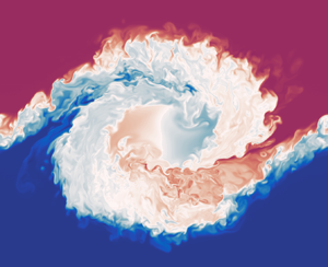
Figure 1. Spanwise slices through  $y=0$ at various indicated times during the flow showing contours of density for simulations: (a)–(d) WN72D; (e)– $(h)$ NM72D; $(i)$– $(l)$ WN72 (in which shear does not decelerate). Only the central region $-5\leq z \leq 5$ is shown.
The KHI billows are well-developed by the time the shear has started to decelerate for both types of initial condition, with a normal-mode perturbation resulting in a more rapid billow development than a white-noise perturbation, as is indicated by the presence of secondary instabilities in figure 1(e) which facilitate the breakdown to turbulence. At this point, the billow shape is already visibly modified for flows which have a deceleration phase as can be seen by comparing figures 1(a) and 1(e) with 1 $(i)$. This modification is primarily due to the influence of the shear, which continues to deform the growing billow in simulation WN72 in which the shear is held constant after acceleration, resulting in a structure that is flatter in the vertical and longer in the horizontal. As a result, the vertical extent of turbulent motions that emerge is larger in flows that decelerate compared with flow WN72. Turbulence is more short-lived in decelerating flows resulting in billow collapse and partial relaminarisation, as can be seen in figures 1(c) and 1(g). However, flow WN72D actually supports a secondary phase of weaker turbulence seen in figure 1(d), which forms above and below the centre of the mostly laminar central region, resulting in a further (vertical) broadening of the mixed layer. The result is that, despite the preceding phase of relaminarisation, the final vertical extent of the mixed layer is similar to that produced by the shear-sustained turbulence of simulation WN72. Similar dynamics is observed for simulations WN52D and WN62D.
To investigate this secondary mixing behaviour further, figure 2 shows the evolution of the quantity  $4N^{2}-S^{2}$, where $N(z,t)$ and $S(z,t)$ are local measures of buoyancy frequency and shear defined by horizontally averaged fields (denoted by an overbar):
 \begin{equation} N^{2} ={-} Ri_b \frac{\partial \bar{\rho}}{\partial z}, \quad S = \frac{\partial \bar{u}}{\partial z}. \end{equation}
Positive and negative values of  $4N^{2}-S^{2}$ correspond to the gradient Richardson number $Ri_g=N^{2}/S^{2}$ being greater than or less than the value of $1/4$ associated with marginal linear instability. The earlier development of KHI is clear in simulations NM72D, WN62D and WN52D, though the horizontally averaged structure remains similar across all simulations until the billow starts to collapse. Values of $Ri_g< 1/4$ are maintained in the centre of the shear layer throughout most of the turbulent mixing event for the reference flow WN72, in contrast to the decelerating flows. For these flows, there are coherent wave-like structures corresponding to larger $Ri_g$ at the top and bottom of the mixing layer which emerge as the shear decelerates. Similar structures were also observed for KHI billows forming in a linear background stratification in Lewin & Caulfield (Reference Lewin and Caulfield2021), caused by anisotropic turbulence rotating around the laminar billow core. Once the shear starts to accelerate again, values of $Ri_g$ in these regions decrease, in particular leading to distinct patches of $Ri_g< 1/4$ in flows WN72D, WN62D and WN52D which leads to the development of a secondary turbulence phase. Similar behaviour for forced stratified shear flows in which $Ri_g$ becomes negative in regions above and below the centre of the shear layer has been observed by Smith, Caulfield & Taylor (Reference Smith, Caulfield and Taylor2021) in simulations that are continuously relaxed towards prescribed mean profiles.

Figure 2. Time evolving vertical profiles of the quantity  $4N^{2}-S^{2}$ for simulations: (a) WN72D; (b) NM72D; (c) WN72; (d) WN62D; (e) WN52D. Regions for which the gradient Richardson number $Ri_g\leq 1/4$ are shown in orange.
3.2. More mixing with less shear
Stratified mixing may be characterised as an irreversible, diffusive process by decomposing the total potential energy  $\mathscr {P}=Ri_b \langle \rho z\rangle$ into the sum of an available potential energy (APE) $\mathscr {P}_A$ and a background potential energy (BPE) $\mathscr {P}_B$ defined by $\mathscr {P}_B\equiv Ri_b\langle \rho _B z\rangle$, where $\rho _B$ is obtained by rearranging the density field adiabatically into a gravitationally stable monotonic configuration. Here, angle brackets denote a volume average over the entire domain. As detailed by Caulfield & Peltier (Reference Caulfield and Peltier2000), it follows that the quantity
 \begin{equation} \frac{\text{d}\mathscr{P}_B}{\text{d}t}=\mathscr{M}+\mathscr{D}_p, \end{equation}
is necessarily monotonically increasing at a rate bounded below by the diffusion of the background density gradient  $\mathscr {D}_p\equiv 2Ri_b/({Re}{Pr}L_z)$. The (strictly non-negative) quantity $\mathscr {M}$ is known as the mixing rate. An (instantaneous) mixing efficiency $\eta$ may then be defined as
 \begin{equation} \eta \equiv \frac{\mathscr{M}}{\mathscr{M}+\varepsilon}, \end{equation}
where  $\varepsilon = \langle \partial _j u_i \partial _j u_i\rangle /{Re}$ is the total kinetic energy dissipation.
Figure 3(a) shows the evolution of the total change in BPE due to irreversible turbulent mixing (which is a measure of the total amount of flow-induced mixing) for each simulation in table 1, calculated by subtracting the time-integrated contribution  $D_p t$ due merely to background diffusion. We compute $\mathscr {P}_B$ by assuming a tilt angle of zero, shown by Inoue & Smyth (Reference Inoue and Smyth2009) to be a reasonable approximation for $a\lesssim 10^{\circ }$. The corresponding values of the change in APE are plotted in figure 3(b). Evolution depends on the forcing frequency $\varOmega$ and the initial flow conditions that determine the timing of the growth of the primary KHI billow. In flows WN62D, WN52D and NM72D, the primary billow develops earlier during the shear oscillation cycle due to the slower forcing frequency or a faster growing normal-mode perturbation. These billows do not store more APE in their initial saturated state than the slower developing billows of flows WN72D and WN72, but nonetheless have a significantly larger total change of BPE by the end of the mixing cycle. Additional energy for mixing comes from a sustained increased volume of APE throughout the mixing cycle; by comparison, flow WN72 reaches a similar initial peak of APE which then quickly drops off. Hence the background shear has a strong influence on how energy is stored in the flow. There are, therefore, three key aspects leading to substantial mixing in decelerating flows. Firstly, the APE stored in these flows remains large throughout the mixing cycle compared with constant shear flows. Secondly, those flows in which a billow develops earlier relative to shear deceleration experience a longer period of sustained large APE. Finally, additional mixing may take place during the second phase of shear acceleration. In this way, it is possible for decelerating flows to mix as much as, or even significantly more than, their constant shear counterparts.

Figure 3. Evolution of (a) change in BPE due to irreversible flow-induced mixing; (b) change in APE; (c) TKE for each simulation in table 1.
There are notable APE oscillations in the absence of shear whose period is observed to be  $2{\rm \pi} \varOmega$. Since $\varOmega = \omega ^{*}/N_b^{*}$ and $T=\omega ^{*}t^{*}$, this corresponds to oscillations at the background buoyancy frequency. To investigate further, figure 3(c) shows the evolution of turbulent kinetic energy (TKE) $(\langle u'^{2}\rangle + \langle v'^{2}\rangle + \langle w'^{2}\rangle )/2$, where $\boldsymbol {u}'=\boldsymbol {u}-\bar {\boldsymbol {u}}$. Perhaps surprisingly, the decelerating flows exhibit similar or greater TKE than flow WN72, despite the additional kinetic energy from the background shear in the latter. This additional TKE appears to come (at least in part) from the APE, whose oscillations are distinctly out of phase with the TKE oscillations in decelerating simulations. There are fundamental differences in the energetics between the oscillating flows and the constant shear flow WN72, but we also note that earlier billow development in flows NM72D, WN62D and WN52D leads to a larger total TKE than flow WN72D, indicating timing also plays an important role in energy transfer.
In order to look at the contributions of different stages of a given mixing event to the total mixing, we define the start of the energetic ‘fully turbulent’ mixing phase to be when the buoyancy Reynolds number  ${Re}_b = {Re}{\langle \varepsilon \rangle }/{\langle N^{2}\rangle }$ first becomes bigger than a nominal critical value of ${Re}_b^{t}=200$. A value of ${Re}_b\sim O(100)$ is commonly associated with the most energetic turbulence found in stratified flows (Shih et al. Reference Shih, Koseff, Ivey and Ferziger2005; Salehipour & Peltier Reference Salehipour and Peltier2015; Portwood et al. Reference Portwood, de Bruyn Kops, Taylor, Salehipour and Caulfield2016), and we find the results in the following discussion are robust for $100\leq {Re}_b^{t} \leq 300$. The value of the tilt phase $T$ corresponding to the start of the energetic mixing phase is denoted $T^{t}$ and is indicated in table 1 for each simulation. Also given is the total overall change in BPE $\Delta \mathscr {P}_B$, as well as the change in BPE over the turbulent and preturbulent mixing phase $\Delta \mathscr {P}_B^{t}$ and $\Delta \mathscr {P}_B^{i}$. It is clear that, at least from using this definition of the turbulent mixing phase, the larger total mixing in simulations NMM72, WN62D and WN52D is due to an increase in both the preturbulent and fully turbulent mixing phases.
Inoue & Smyth (Reference Inoue and Smyth2009) argue that time-dependent forcing governs the mixing by altering the relative duration of these two phases, with shear deceleration essentially suppressing less efficient fully turbulent mixing, so that the preturbulent mixing dominates. Although a reasonable description at low to moderate  ${Re}$, at higher ${Re}$, a description of shear-induced turbulence as being controlled by the relative duration between efficient preturbulent and less efficient fully turbulent mixing is insufficient to describe the event in generality because the fully turbulent mixing stage is relatively much more important.
3.3. Energy pathways
Having established the importance of  $\varOmega$ in determining the timing of the shear deceleration phase for the mixing of the system, we will henceforth focus on simulations with $\varOmega =0.072$ to investigate the mechanisms and energetic pathways that lead to the time-dependent behaviour described in the previous section. As illustrated by figure 4(a), the volume-averaged dissipation rate $\varepsilon$ (vertically averaged over $L_z$) reaches a similar order of magnitude for all three simulations, further indicating that the turbulence reaches a similar intensity regardless of whether or not the shear is decelerated. Despite this, there are noticeable differences in the behaviour of the mixing rate $\mathscr {M}$ shown in figure 4(b). In particular, decelerating flows WN72D and NM72D exhibit strong initial peaks followed by rapid decrease in mixing rate at around $T=2{\rm \pi}$. The constant shear flow WN72 instead exhibits a similarly strong initial peak, but then starts to decrease much more gradually than the decelerating flows, with moderate mixing being sustained for a relatively long period of time. These differences are reflected in the behaviour of the mixing efficiency $\eta$ seen in figure 4(c). Once again, the peak values reached during the preturbulent ‘roll-up’ phase are similar across all simulations. However, once the transition to turbulence is initiated by the proliferation of secondary instabilities, mixing efficiency remains considerably higher in simulations WN72D and NM72D, settling at a value of $\eta$ around 0.4, as opposed to the value $\eta \approx 0.2$ in simulation WN72 which matches efficiencies found in constant shear studies of KHI turbulence (Mashayek & Peltier Reference Mashayek and Peltier2013; Salehipour & Peltier Reference Salehipour and Peltier2015; Mashayek et al. Reference Mashayek, Caulfield and Peltier2017). Olson et al. (Reference Olson, Larsson, Lele and Cook2011) obtain similar values of $\eta \approx 0.4$ in their study of combined Rayleigh–Taylor/Kelvin–Helmholtz instability for strong background shear, finding in general that higher shear results in a significant reduction in mixing efficiency of a gravitationally unstable flow. Indeed, at high Reynolds number, a coherent KHI billow supports both shear instability due to the background flow and the rotation of the vortex, and convective instability due to overturning of the density field. We note that the mixing properties of flows WN62D and WN52D evolve in a similar manner to flow NM72D due to the earlier relative development of the billow and so are not shown here. There is a clear indication that, despite initially similar mixing properties associated with the coherent saturated billow state, ensuing turbulence is characteristically different in the absence of a sustaining background shear.

Figure 4. Time evolution of (a) volume-averaged dissipation  $\varepsilon$; (b) mixing rate $\mathscr {M}$; (c) mixing efficiency $\eta$. Plots (d–f) show selected terms from the three-dimensional kinetic energy evolution equation. All simulations have $\varOmega =0.072$.
The argument that turbulence is characteristically different in flows where the shear undergoes deceleration once a primary overturning has developed can be extended further by performing a three-dimensional Reynolds decomposition of the velocity and density fields. Specifically, we write
 $$\begin{gather} \boldsymbol{u}(x,y,z,t) = (u,v,w) = (\bar{u}(z,t)+u_{2d}+u_{3d}, v_{3d}, w_{2d}+w_{3d}), \end{gather}$$
 $$\begin{gather}\boldsymbol{u}_{2d}(x,z,t) = (u_{2d}, 0, w_{2d}) = \langle( u - \bar{u}, v, w)\rangle_y, \end{gather}$$
 $$\begin{gather}\boldsymbol{u}_{3d}(x,y,z,t) = (u_{3d}, v_{3d}, w_{3d}) = (u-u_{2d}-\bar{u}, v, w-w_{2d}), \end{gather}$$
where  $\langle \boldsymbol {\cdot } \rangle _p$ denotes spatial averaging in the coordinate direction(s) $p$. A similar decomposition $\rho (x,y,z,t)=\bar {\rho }(z,t) + \rho _{2d}(x,z,t)+\rho _{3d}(x,y,z,t)$ can be obtained in the same manner. This decomposition represents the mean background flow, along with two-dimensional components associated primarily with the initial KHI billow, and an inherently three-dimensional component that grows in magnitude as small-scale turbulence develops. The evolution equation for the inherently three-dimensional kinetic energy $\mathscr {K}_{3d}=\langle |\boldsymbol {u}_{3d}^{2}|\rangle /2$ is found to have the form (see e.g. Mashayek, Caulfield & Peltier Reference Mashayek, Caulfield and Peltier2013)
 \begin{equation} \frac{\text{d}\mathscr{K}_{3d}}{\text{d}t} = \mathscr{R}_{3d} + \mathscr{S}h_{3d} + \mathscr{A}_{3d} - \mathscr{H}_{3d}-\mathscr{D}_{3d}, \end{equation}
where  $\mathscr {R}_{3d}$ represents the production of $\mathscr {K}_{3d}$ by the background shear, $\mathscr {S}{h}_{3d}$ represents energy sourced from the inherently two-dimensional component of the flow, $\mathscr {A}_{3d}$ is a measure of anisotropy representing energy sourced from stretching deformations, and $\mathscr {H}_3d$ and $\mathscr {D}_{3d}$ are buoyancy flux and dissipation terms associated with three-dimensional perturbations. These terms are explicitly defined as
 $$\begin{gather} \mathscr{R}_{3d} ={-}\left\langle u_{3d}w_{3d}\frac{\partial \bar{u}}{\partial z} \right\rangle , \quad \mathscr{H}_{3d} = Ri_b\langle \rho_{3d}w_{3d}\rangle,\quad \mathscr{D}_{3d} = \langle \partial_j u_{3d_{i}} \partial_j u_{3d_{i}} \rangle, \end{gather}$$
 $$\begin{gather} \mathscr{A}_{3d} ={-}\frac 12\left\langle(u_{3d}^{2}-w_{3d}^{2})\left(\frac{\partial u_{2d}}{\partial x}-\frac{\partial w_{2d}}{\partial z}\right)\right\rangle, \end{gather}$$
 $$\begin{gather}\mathscr{S}h_{3d} ={-}\left\langle u_{3d}w_{3d}\left(\frac{\partial w_{2d}}{\partial x} + \frac{\partial u_{2d}}{\partial z} \right)\right\rangle. \end{gather}$$
Figures 4(d)–4( f) show the evolution of the first three terms on the right-hand side of (3.7) for the three simulations with  $\varOmega =0.072$. Figure 4(d) shows that flow WN72 which does not have a deceleration phase sources the majority of its energy for three-dimensional velocity perturbations from the background shear, as discussed by Caulfield & Peltier (Reference Caulfield and Peltier2000). This is in noticeable contrast to the decelerating flows WN72D and NM72D, for which $\mathscr {R}_{3d}$ is essentially negligible throughout the primary turbulent mixing event. Figures 4(e) and 4( f) show that the energy for three-dimensional velocity fluctuations associated with fully developed turbulence instead comes from a mixture of $\mathscr {S}h_{3d}$ and $\mathscr {A}_{3d}$, both of which do not generally contribute positively to $\mathscr {K}_{3d}$ in the constant shear case. These terms are inherently associated with the motion of the primary KHI billow that develops, suggesting that the deceleration of the background shear provides a direct route to turbulence from the static instability of the billow structure itself. This is consistent both with the qualitative picture of the background shear continuing to deform the billow and subsequent turbulent structures as they develop, and the mixing being more convectively driven with a larger associated mixing efficiency. Importantly, there is no evidence of an intermediate or transitional regime despite shear still being present at the time of turbulent breakdown. Therefore, we conclude that the energy pathways leading to three-dimensional turbulent velocity fluctuations and hence energetic mixing are profoundly modified for these flows.
4. Discussion and conclusions
We have investigated the turbulent mixing produced by KHI in a stratified flow with time-dependent forcing designed to induce a periodically accelerating and decelerating background shear. At sufficiently high  $Re$, the density and velocity fields are organised such that multiple turbulent transitions and hence additional mixing phases are possible as the local gradient Richardson number $Ri_g(z,t)$ becomes smaller than the classical value of $1/4$ associated with instability. By varying the forcing frequency $\varOmega$ and the structure of the initial conditions, we found that both the mixing efficiency and total amount of mixing can in fact be significantly higher for turbulence produced by KHI billows in the absence of background shear that would otherwise act to sustain energetic turbulence. This is essentially due to two main effects. Firstly, and as originally noted by Inoue & Smyth (Reference Inoue and Smyth2009), billows that develop earlier relative to the shear deceleration spend longer in a coherent, preturbulent state associated with highly efficient mixing. Secondly, the energetic pathways leading to mixing are profoundly modified in the absence of shear such that turbulent fluctuations have a characteristically different structure whilst remaining just as energetic as flows with a constant background shear. This latter effect becomes more important as $Re$ increases, and it reinforces the idea that a purely two-phase description of turbulence produced by shear instability consisting of a coherent preturbulent phase of highly efficient mixing followed by an energetic phase of constant mixing efficiency of $\eta \approx 0.2$ does not appropriately characterise the mixing (Mashayek & Peltier Reference Mashayek and Peltier2013), even when the final decaying phase of flow evolution does not play a significant role (Lewin & Caulfield Reference Lewin and Caulfield2021). Mashayek et al. (Reference Mashayek, Caulfield and Alford2021b) point out that mixing by KHI might be more appropriately characterised as primarily convective once the primary billow has rolled up. The analysis of the simulations with decelerating shear in this work highlights the competing nature between shear instabilities and convective gravitational instabilities of the KHI billow, with the latter potentially giving rise to much more efficient mixing. We anticipate that this reasoning will apply to more general overturning structures in the ocean. Indeed, Howland et al. (Reference Howland, Taylor and Caulfield2021) find a similar competition between shear and convective instabilities in the interaction between a large-scale breaking gravity wave and a background sinusoidal shear flow.
Although we have not focused on specific parameterisation issues in this work, here it is worth pointing out some of the implications for models of mixing efficiency used to predict diapycnal diffusivity from measurable quantities in the ocean (Gregg et al. Reference Gregg, D'Asoro, Riley and Kunze2018). Clearly, transient effects are important for determining mixing efficiency in the sense that the mechanisms driving turbulence have a strong influence on the resulting mixing behaviour. Our results support the argument that at least some estimate of the APE stored in the flow is necessary for a reasonable understanding of inherently time-dependent turbulent mixing behaviour, as has been recently argued by Mashayek et al. (Reference Mashayek, Baker, Cael and Caulfield2021a) by considering the relative size of the Ozmidov and Thorpe scales  $L_O$ and $L_T$ in the flow. Here $L_O=(\varepsilon /N^{3})^{1/2}$ quantifies the size of the largest turbulent eddies unaffected by stratification, whilst $L_T$ is an overturning scale obtained from the displacements required to reorder a vertical profile of density into a monotonically decreasing profile. This work indicates that the relative importance of the shear also plays a role that is more complex than a simple dependence on the classical criterion of the gradient Richardson number $Ri_g$ being less than $1/4$. A natural length scale associated with the shear is the Corrsin scale $L_S = (\varepsilon /S^{3})^{1/2}$, where $S$ is the vertical shear of the mean horizontal velocity. As argued by Ivey, Bluteau & Jones (Reference Ivey, Bluteau and Jones2018), consideration of the relationship between all three of these length scales might be useful for better constraining parameterisations of mixing efficiency. Finally, it is important to note that, whilst this study focused on the specific effects of timing, varying other key parameters such as $Ri_b$ and $Pr$ may also play an important role in determining the evolution of the structure and mixing of the flow. The role of transient flow dynamics such as those described here in adding uncertainty to parametrizations of mixing, and attempting to characterise these uncertainties, is an important consideration for future studies.
Supplementary movie
Supplementary movie is available at https://doi.org/10.1017/jfm.2022.537.
Acknowledgements
The authors are grateful for the helpful comments from two reviewers which had a significant positive impact on the manuscript. The data and code for producing the figures is available at https://github.com/samlewin/oscillating_shear
Funding
This work has been performed using resources provided by the Cambridge Tier-2 system operated by the University of Cambridge Research Computing Service (www.hpc.cam.ac.uk) funded by EPSRC Tier-2 capital grant EP/P020259/1. S.F.L. is supported by an Engineering and Physical Sciences Research Council studentship from UKRI.
Declaration of interests
The authors report no conflict of interest.


 Open access