


1. Introduction
A compression shock from an adverse pressure gradient impinging on a hypersonic boundary layer may cause flow reversal if the pressure gradient is strong enough. This shock/boundary-layer interaction (SBLI) forms a separation bubble in the flow. The local flow properties, such as pressure and boundary layer state, determine the extent and evolution of such a bubble. Understanding how an SBLI bubble affects boundary-layer transition is essential for hypersonic vehicle design, as frequently this phenomenon occurs at compression corners such as those near control surfaces, and transition has a large effect on local surface heating. However, the existence of a separation bubble is influenced by transition, which itself is influenced by the presence of the bubble, forming a complex coupled problem.
Research into transitional SBLI separation began in the 1950s, when Becker & Korycinski (Reference Becker and Korycinski1956) experimented with an ogive-cylinder-flare at Mach 6.8. Their results showed large separation bubbles under laminar flow that decreased in size as the transition point shifted upstream of reattachment. Initial transitional SBLI studies focused on mean flow trends and conditions affecting separation bubble geometry. Chapman, Kuehn & Larson (Reference Chapman, Kuehn and Larson1958) were the first to observe the ‘free interaction’ of the boundary layer with the external supersonic flow. Increasing the Mach number or freestream unit Reynolds number were both found to result in a larger bubble (Chapman et al. Reference Chapman, Kuehn and Larson1958; Larson & Keating Reference Larson and Keating1960; Needham & Stollery Reference Needham and Stollery1966); however, the Reynolds number trend reverses when transition moves upstream of the reattachment point (Needham & Stollery Reference Needham and Stollery1966; Heffner, Chpoun & Lengrand Reference Heffner, Chpoun and Lengrand1993).
The cone-cylinder-flare geometry was originally experimented with by Schaefer & Ferguson (Reference Schaefer and Ferguson1962), who documented separation, reattachment and heat flux trends with changing freestream Reynolds number. Ginoux (Reference Ginoux1965), who used both a hollow cylinder-flare and a version with a sharp conical nose, noted that streamwise vortices present on the flare downstream of reattachment were less observable with the sharp nose. He noted that leading-edge sensitivity may amplify instabilities leading to those vortices, and suggested that future axisymmetric SBLI work should utilize a sharp, slender model to avoid such sensitivity. The present study uses a sharp cone-cylinder-flare, with this particular geometry designed originally by Esquieu et al. (Reference Esquieu, Benitez, Schneider and Brazier2019), for this reason.
A 1990 review on high-speed shear-layer transition determined that more measurements of laminar instabilities present in the shear layer and what effect they might have on transition were necessary (Demetriades Reference Demetriades1990). SBLI separation-induced instability and transition have therefore been the focus of numerous recent hypersonic studies. In particular, significant effort has been made to understand the streamwise streaks visible around reattachment in SBLI flows (Heffner et al. Reference Heffner, Chpoun and Lengrand1993; Benay et al. Reference Benay, Chanetz, Mangin, Vandomme and Perraud2006; Dwivedi et al. Reference Dwivedi, Sidharth, Candler, Nichols and Jovanovic2018; Leinemann et al. Reference Leinemann, Radespiel, Muñoz, Esquieu, McKiernan and Schneider2019; Li et al. Reference Li, Choudhari, Paredes and Scholten2022; Wagner Reference Wagner2022; Cao et al. Reference Cao, Hao, Klioutchnikov, Wen, Olivier and Heufer2022), first noted by Ginoux (Reference Ginoux1965), as well as the role of the bubble in transition location (Dwivedi et al. Reference Dwivedi, Sidharth, Candler, Nichols and Jovanovic2018; Vandomme et al. Reference Vandomme, Chanetz, Benay and Parraud2003).
Study of the high-frequency fluctuations on hypersonic SBLIs has become the focus of modern aerodynamic research. For flat plates or slender geometries at hypersonic speeds, the second (Mack) mode (Mack Reference Mack1975) is known to be the dominant instability leading to transition (Fasel, Thumm & Bestek Reference Fasel, Thumm and Bestek1993; Chang & Malik Reference Chang and Malik1994). Adams (Reference Adams2001) was the first to show that the second mode did not amplify over a laminar separation bubble with direct numerical simulations of a compression ramp at Mach 5. Later, Balakumar, Zhao & Atkins (Reference Balakumar, Zhao and Atkins2005) studied numerically the lower surface of the Hyper-X model, which included a compression corner. Their findings showed that the second mode amplified prior to separation, and then convected downstream in the shear layer while maintaining its pre-separation amplitude, implying that this instability is neutrally stable in the shear layer (similar to Adams Reference Adams2001). The second mode then proceeded to amplify in the boundary layer downstream of reattachment. The effect of intermittent turbulent spots on hypersonic separation bubbles has also been studied (Estruch-Samper et al. Reference Estruch-Samper, Ganapathisubramani, Vanstone and Hiller2012; Vanstone et al. Reference Vanstone, Estruch-Samper, Hillier and Ganapathisubramani2013, Reference Vanstone, Estruch-Samper, Hillier and Ganapathisubramani2017; Vanstone & Clemens Reference Vanstone and Clemens2019). Most recently, Estruch-Samper, Hiller & Vanstone (Reference Estruch-Samper, Hiller and Vanstone2022) used a roughness element on a blunt cylinder-flare, which produced isolated turbulent spots, to study the collapse and re-establishment of a laminar separation bubble at Mach 9. They found that the local separation responds to the spot rapidly, while bubble re-establishment may take as long as four times the spot transit time. With a small (approximately 23 mm long) separation bubble and a relatively high Mach number, they measured bubble re-establishment to take about 2 ms. However, previous testing with a cone-cylinder-flare in Mach-6 flow by Benitez et al. (Reference Benitez, Borg, Paredes, Schneider and Jewell2023), which had a larger bubble (estimated between 150 and 180 mm long) and a lower Mach number than Estruch-Samper et al. (Reference Estruch-Samper, Hiller and Vanstone2022), found initial bubble establishment times to be of the order of 10 ms. With such long establishment times, hypersonic separation bubbles studied in short-duration impulse facilities may never reach steady-state conditions.
While low-speed studies have shown previously that unsteadiness of the shear layer itself could lead to transition downstream of reattachment (Dovgal, Kozlov & Michalke Reference Dovgal, Kozlov and Michalke1994), similar shear-layer-related unsteadiness has only recently been investigated in the hypersonic regime. McKiernan & Schneider (Reference McKiernan and Schneider2021) conducted a series of experiments in the Boeing/AFOSR Mach-6 Quiet Tunnel (BAM6QT) at Purdue. They tested an Oberkampf cone-slice-flap geometry (Oberkampf & Aeschliman Reference Oberkampf and Aeschliman1992) under quiet flow with a variety of flap deflection angles, with the purpose of measuring pressure fluctuations directly downstream of reattachment. Transition was observed under quiet flow, but only through a broadband increase in the surface pressure power spectra, rather than through instability amplification and breakdown. By introducing artificial disturbances to the boundary layer upstream of the separation, they were able to see a convective instability in the reattached boundary layer. However, they determined that the cause of transition on the model was independent of this instability. Pandey et al. (Reference Pandey, Casper, Guildenbecher, Beresh, Bhakta, De Zetter and Spillers2022) continued work on this geometry at Mach 8 under conventional noise levels with several additional measurement techniques. Using both high-speed schlieren and a scanning focused laser differential interferometry (FLDI) technique, they measured both the second mode as well as lower-frequency fluctuations related to a shear-layer instability. Additional study of this geometry focused on the expansion corner found that the expansion had a stabilizing effect on the boundary-layer fluctuations, to the point where relaminarization is hypothesized to occur (Pandey et al. Reference Pandey, Jirasek, Saltzman, Casper, Beresh, Bhakta, Denk, De Zetter and Spillers2023).
Lugrin et al. (Reference Lugrin, Beneddine, Leclercq, Garnier and Bur2021) published a detailed computational study of a transitional SBLI caused by a  $15^{\circ }$ axisymmetric ramp at Mach 5. Utilizing spectral proper orthogonal decomposition (SPOD), they determined that transition on that geometry was caused by the linear amplification of oblique modes that interact nonlinearly, creating the streamwise striations observed frequently in experiments. The next year, Lugrin et al. (Reference Lugrin, Nicolas, Severac, Tobeli, Beneddine, Garnier, Esquieu and Bur2022) published their experimental findings on a hollow cylinder-flare with a sharp leading edge at the R2Ch blowdown tunnel at ONERA. Using heat transfer measurements, they observed clear streaks under the reattached boundary layer at various wavenumbers. Their SPOD analysis on high-speed schlieren imagery indicated that oblique shear layer modes were dominant over the separated region. The study focused on a transitional separation bubble, which was laminar at separation but transitional at reattachment, and was conducted at three different freestream unit Reynolds numbers. Recent computational investigation of convective and global boundary-layer instabilities over a sharp cone-cylinder-flare model at Mach 6 by Paredes et al. (Reference Paredes, Scholten, Choudhari, Li, Benitez and Jewell2022) captured the distinct lobes within the disturbance amplification spectra measured with wall-pressure sensors at the BAM6QT with $10^\circ$ flare, and reported that the oblique Mack's first-mode waves that begin to amplify over the cone continue to grow along the separated shear layer. Weakly nonlinear input–output analysis and direct numerical simulations by Dwivedi, Sidharth & Jovanovic (Reference Dwivedi, Sidharth and Jovanovic2022) for a globally stable double wedge flow at Mach 5 discussed that shear stress fluctuation due to streamline curvature as the physical mechanism for the amplification of the oblique waves.
Butler & Laurence (Reference Butler and Laurence2021) studied axisymmetric expansion and compression corners in the University of Maryland HyperTERP hypersonic shock tunnel. Using a  $5^{\circ }$ half-angle sharp cone with a $0^{\circ }$ and $15^{\circ }$ flare, they acquired high-speed schlieren images and surface pressure fluctuation data. Butler found that energy was being radiated away from the second-mode instability in the shear layer over the separation bubble for the $15^{\circ }$ flare. The next year, they published the results sweeping compression angles and Reynolds numbers, highlighting the increase in dominance of the shear-layer instability with increasing flare angle (Butler & Laurence Reference Butler and Laurence2022). Their bubble can be classified as transitional, as the reattachment point moved upstream with increasing unit Reynolds number (Becker & Korycinski Reference Becker and Korycinski1956). Butler & Laurence (Reference Butler and Laurence2022) have stated the need to study the shear-layer instability in a facility with longer run times and higher-quality flow; this work helps to fill that gap.
Previous work by Benitez et al. (Reference Benitez, Jewell, Schneider and Esquieu2020) first documented a naturally occurring convective hypersonic shear-layer instability (which was termed the ‘shear-generated’ or ‘shear-layer’ instability) over a sharp cone-cylinder-flare geometry with a  $10^{\circ }$ flare angle. Their experimental campaign had a fully laminar separation bubble. Under quiet flow with the $10^{\circ }$ flare, the shear-layer instability was observed in both surface pressure fluctuation measurements and off the surface with FLDI. The second mode was also observed in the boundary and shear layers. The shear-layer instability appeared to be neutrally stable in the reattached boundary layer, while the second mode amplified downstream of reattachment along the flare. Transition onset was not observed due to limitations in the maximum quiet unit Reynolds number. Introduction of a broadband, large-amplitude initial disturbance via plasma perturbation downstream of the cone but upstream of the separation led to amplified shear-layer waves that appeared to devolve into turbulent-spot-like structures in the reattached boundary layer (Benitez, Jewell & Schneider Reference Benitez, Jewell and Schneider2021). Computational analysis by Paredes et al. (Reference Paredes, Scholten, Choudhari, Li, Benitez and Jewell2022) indicated that a slightly larger flare angle might make the shear and boundary layers sufficiently unstable to transition under low-disturbance flow without such artificial methods.
The present study expands on the previous  $10^{\circ }$ cone-cylinder-flare campaign made at Mach-6 under quiet flow by presenting results from a cone-cylinder-flare with a larger, $12^{\circ }$ flare angle. It provides the first experimental results for transition onset with a laminar SBLI separation bubble under low-disturbance flow; the data suggest that turbulent spots generated downstream of reattachment are likely triggered by the shear-layer instability, rather than the second mode alone. A linear numerical stability analysis has also been performed, which supports the behaviour of the instabilities observed in the experimental data.
2. Experimental set-up
2.1. Boeing/AFOSR Mach-6 Quiet Tunnel (BAM6QT)
Hypersonic experiments were conducted in the Boeing/AFOSR Mach-6 Quiet Tunnel (BAM6QT) at Purdue University. The BAM6QT is a Ludwieg tube that is capable of being run with conventional noise or quiet flow with run times up to 6 s. It consists of a 40.8 m driver tube connected to a converging–diverging nozzle that exhausts into a 113 cubic metre vacuum tank. The test section is located in the downstream end of the diverging section of the nozzle, and includes optical access with contoured Plexiglas or flat sapphire or calcium fluoride windows. The large sapphire windows are used primarily for schlieren imagery, while the smaller calcium fluoride ones are used with infrared thermography, although they can also be used for schlieren. A basic illustration of the facility is given in figure 1.

Figure 1. BAM6QT schematic.
To obtain quiet flow, a combination of several features is implemented to reduce disturbances and keep the boundary layer on the nozzle laminar. The nozzle of the BAM6QT is polished to a mirror finish to reduce the presence of roughness on the surface. Additionally, the nozzle itself is long such that the radius of curvature in the streamwise direction is large, reducing amplification of the Görtler instability. Air travels through a particle filter before entering the driver tube to remove most particles, such that the air is similar to that in a clean room. Finally, bleed slots are located at the throat of the nozzle. These slots use suction to remove the boundary layer from the nozzle so it begins again at the throat, thereby removing any disturbances that might convey from the contraction section. Together, those features allow the tunnel to operate with very low freestream noise levels of less than 0.02 % (Mamrol & Jewell Reference Mamrol and Jewell2022). These low-disturbance freestream fluctuation levels are similar to flight (Juliano, Swanson & Schneider Reference Juliano, Swanson and Schneider2007; Schneider Reference Schneider2008, Reference Schneider2015). However, at high enough Reynolds numbers, the flow will still be noisy. For these experiments, the tunnel was capable of operating quietly at up to unit Reynolds number approximately  $14.3\times 10^6\ {\rm m}^{-1}$. However, due to pressure restrictions, the large sapphire windows were capable of being used for schlieren only up to $Re_\infty =12.8\times 10^6\ {\rm m}^{-1}$. Therefore, schlieren data were restricted to that freestream unit Reynolds number; higher Reynolds number data were still collected with PCB and Kulite sensors. Prior measurements made with the 10 $^{\circ }$ flare model had maximum quiet unit Reynolds number $Re_\infty =12.0\times 10^6\ {\rm m}^{-1}$ due to tunnel limitations at the time of testing.
2.2. Surface pressure sensors
Surface pressure fluctuation measurements were acquired with PCB132B38 sensors as well as Kulite XCE-062-15A sensors. The PCB sensors were manufactured by PCB Piezotronics. These sensors are high-pass filtered above 11 kHz and have high-frequency response limit 1 MHz. The PCB sensors have nominal resolution 7 Pa, with rise time less than  $3\ \mathrm {\mu }{\rm s}$. The PCB factory calibrations provide a single number to convert voltages to pressure fluctuations; this value was used to scale the voltages to pressure measurements.
Kulite XCE-062-15A sensors were used to acquire lower-frequency disturbances. These transducers are smaller than PCBs, with a 1.7 mm diameter, but have a slower response time. This lower response time, coupled with the sensor's large resonance peak, restrict their useful frequency content to below 270 kHz. A custom signal conditioning box was used to power the Kulites with two outputs; the DC-coupled output had gain 100 $\times$, while the AC-coupled output had gain 10 000 $\times$.
Data taken with the PCB sensors and the Kulite DC signals were sampled at 5 MHz with an HBM data acquisition system, and analogue low-pass filtered at 1.25 MHz to preclude aliasing. For Kulite AC signals, the data were sampled at 2 MHz with wideband filtering. While both Kulite and PCB data were taken, the Kulite results were comparable to the PCBs, so only the PCB outputs are shown in this paper.
2.3. High-speed schlieren imaging
Schlieren imaging was used both to visualize the time-averaged bubble geometry and study the instabilities along the shear layer and reattached boundary layer. A Phantom TMX 7510 high-speed camera captured the images from a Z-type schlieren apparatus with 8 inch parabolic mirrors. Lighting was provided by a Cavilux SMART high-speed illumination system with pulse lengths set to 10 ns. Images were taken at frame rates between 100 and 875 kHz, with higher frame rates collecting only a discrete number of image bursts, while the 100 kHz rate was capable of obtaining images of the duration of the run.
As the schlieren utilized in this experiment was uncalibrated, plots with schlieren data are in arbitrary units that correspond to the individual pixel intensity values captured by the camera. Schlieren as a measurement technique captures the density gradients in the flow, but without calibration dimensional amplitudes cannot be accurately applied to the measurements. Therefore, the data refer simply to a generic ‘schlieren intensity’.
2.4. Model and instrumentation
The axisymmetric compression corner model consists of a cone-cylinder-flare geometry based on the design by Esquieu et al. (Reference Esquieu, Benitez, Schneider and Brazier2019). It is divided into three components, with a stainless steel nosetip, aluminum cone-cylinder (with a  $5^{\circ }$ half-angle for the cone), and PEEK cylinder-flare ( $12^{\circ }$ half-angle conical flare). In addition to a sharp (radius 0.1 mm) nosetip, two blunt nosetips were manufactured (radii 1 mm and 5 mm).
Figure 2 shows an illustration of the model. There are ports for up to 18 PCB sensors, with 15 along the central sensor ray (azimuthal angle  $180^{\circ }$) and 3 located azimuthal angles, 0 $^{\circ }$, 90 $^{\circ }$ and 270 $^{\circ }$. Additionally, there are 27 ports for Kulite sensors, with 12 located 30 $^{\circ }$ from the main ray. The remaining 15 are divided into three groups of five sensors that span the azimuth between the PCB and Kulite rays (between 180 $^{\circ }$ and 210 $^{\circ }$). These sensors are separated by 5 $^{\circ }$ azimuthally and by 25.4 mm in the streamwise direction.

Figure 2. Illustration of the 12 $^{\circ }$ cone-cylinder-flare model used in the experiments. Dimensions are in millimetres.
The sideslip angle and angle of attack for the model were zeroed using four PCB sensors located 90 $^{\circ }$ apart azimuthally at the same downstream location along the 5 $^{\circ }$ cone. The second-mode peak frequency was determined at each of these sensors. When at 0.0 $^{\circ }$, the peak frequencies from all four sensors should theoretically be the same. In practice, the model was adjusted until the four peaks were within 4 % of the mean peak frequency.
For this set of experiments, only the sharp nosetip was utilized. PCB stations along the flare were used primarily for the surface pressure fluctuation analysis, although Kulite measurements were also taken.
A similar 10 $^{\circ }$ flare model has been extensively tested previously at the BAM6QT. A subset of results from that model are included in this paper for comparison purposes. An illustration of the 10 $^{\circ }$ flare model is given in figure 3, and more information about its design and experimental campaign can be found in Benitez (Reference Benitez2021). Note that it has a shorter cylinder section, as the 12 $^{\circ }$ flare was predicted to require a longer section to allow the flow to separate downstream of the expansion corner. Additionally, the 10 $^{\circ }$ model has a longer flare; since both models were limited in their base diameter to prevent tunnel blockage issues, the larger angle naturally required a shorter flare.

Figure 3. Illustration of the 10 $^{\circ }$ cone-cylinder-flare model used in the prior experiments (Benitez et al. Reference Benitez, Borg, Paredes, Schneider and Jewell2023). Dimensions are in millimetres.
3. Computational set-up
In this study, a numerical stability analysis was performed to bolster the experimental findings. The axisymmetric laminar flow solution over the cone-cylinder-flare geometry was calculated to study the amplification of linear convective and global instabilities.
3.1. Laminar flow solution
The laminar flow solutions were obtained using the second-order-accurate finite-volume compressible Navier–Stokes flow solver VULCAN-CFD (Litton, Edwards & White Reference Litton, Edwards and White2003; visit http://vulcan-cfd.larc.nasa.gov for further information about the VULCAN-CFD solver). This solver is based on the full Navier–Stokes equations and has the capability to adapt the computational grid iteratively to the bow shock and the boundary layer, as described in Scholten et al. (Reference Scholten, Paredes, Li, White, Baurle and Choudhari2022). The adaptation process ensures adequate resolution of the boundary layer and within the separation region by clustering enough points next to the model surface. The boundary-layer edge was defined as the wall-normal position where  $h_t/h_{t,\infty }=0.99$, with $h_t$ representing the total enthalpy. This is calculated as $h_t=h+0.5(\bar {u}^2+\bar {v}^2+\bar {w}^2)$, with $h=c_p \bar {T}$ being the static enthalpy. An offset was applied to ensure proper resolution of the entropy layer, and dynamic viscosity was calculated using Sutherland's law for air as a function of temperature. An isothermal wall with $T_{wall}=300$ K was used, and freestream conditions were selected to match one of the experimental runs, as listed in table 1. The computational grid consisted of $3601\times 1201$ points along the streamwise and wall-normal directions, respectively. The selected grid resolution follows the previous calculations for the same geometry and similar conditions by Paredes et al. (Reference Paredes, Scholten, Choudhari, Li, Benitez and Jewell2022).
Table 1. Flow conditions used for the computational results of the sharp cone-cylinder-flare.

3.2. Linear stability analysis
The present work is focused on the boundary and shear layers over an axisymmetric body in a hypersonic flow. The overall numerical procedure used for the convective and global instability analysis in the present paper is similar to that used by Paredes et al. (Reference Paredes, Scholten, Choudhari, Li, Benitez and Jewell2022) for the same geometry. However, a succinct summary is provided herein for the purposes of completeness. The Cartesian coordinates are represented by  $(x,y,z)$. For this problem, the computational coordinates are defined as an orthogonal, body-fitted coordinate system, with $(\xi,\eta,\zeta )$ denoting the streamwise, wall-normal and azimuthal coordinates, respectively, and $(u,v,w)$ representing the corresponding velocity components. Density and temperature are denoted by $\rho$ and $T$, respectively. The vector of flow variables ${\boldsymbol {q}}(\xi,\eta,\zeta,t)=(\rho,u,v,w,T)^{\rm T}$ is decomposed into a vector of stationary basic state variables $\bar {\boldsymbol {q}}(\xi,\eta,\zeta )=(\bar {\rho },\bar {u},\bar {v},\bar {w},{\bar {T}})^{\rm T}$ and a vector of perturbation variables $\tilde {\boldsymbol {q}}(\xi,\eta,\zeta,t)=(\tilde {\rho },\tilde {u},\tilde {v},\tilde {w},\tilde {T})^{\rm T}$. For axisymmetric geometries at zero degrees angle of attack, the basic state variables are independent of the azimuthal coordinate, and the linear perturbations can be assumed to be harmonic in time and in the azimuthal direction, which leads to the following expression for the perturbations:
 \begin{equation} \tilde{\boldsymbol{q}}(\xi,\eta,\zeta,t)=\breve{\boldsymbol{q}}(\xi,\eta) \exp\left[{\rm i} (m\zeta-\omega t)\right]+{\rm c.c.}, \end{equation}
where the vector of disturbance functions is  $\breve {\boldsymbol {q}}(\xi,\eta,\zeta )=(\breve {\rho },\breve {u},\breve {v},\breve {w},\breve {T})^{\rm T}$, $m$ is the azimuthal wavenumber, $\omega$ is the angular frequency and ${\rm c.c.}$ refers to the complex conjugate.
The disturbance functions  $\breve {\boldsymbol {q}}(\xi,\eta,\zeta )$ satisfy the harmonic linearized Navier-Stokes equations (HLNSE; Paredes et al. Reference Paredes, Choudhari, Li, Jewell, Kimmel, Marineau and Grossir2019), which involve coefficient functions that depend on the basic state variables and parameters, and on the angular frequency and azimuthal wavenumber of the perturbation.
The parabolized stability equations (PSE) approximation to the HLNSE is based on isolating the rapid phase variations in the streamwise direction by introducing the disturbance ansatz
 \begin{equation} \breve{\boldsymbol{q}}(\xi,\eta,\zeta)=\hat{\boldsymbol{q}}(\xi,\eta,\zeta) \exp\left[ {\rm i} \int_{\xi_0}^{\xi}\alpha(\xi')\,{\rm d}\xi'\right], \end{equation}
where the unknown, streamwise varying wavenumber  $\alpha (\xi )$ is determined in the course of the solution by imposing an additional constraint to require the amplitude functions to vary slowly in the streamwise direction.
The initial condition ( $\hat {\boldsymbol {q}}$ and $\alpha$) for the PSE integration is calculated with the quasi-parallel linear stability theory analysis at the neutral location $\xi _{I}$ of the corresponding $(\omega,m)$ combination.
The onset of laminar–turbulent transition is estimated by using the logarithmic amplification ratio, the so-called N-factor, relative to the location  $\xi _{I}$ where the disturbance first becomes unstable:
 \begin{equation} N_\phi=-\int_{\xi_{I}}^{\xi}\alpha_i(\xi')\,\mathrm{d}\xi'+\ln\left[\hat{\phi}(\xi)/\hat{\phi}(\xi_{I})\right]. \end{equation}
Here,  $\hat {\phi }$ denotes an amplitude norm of $\hat {\boldsymbol {q}}$ at a given $\xi$, e.g. wall-pressure disturbance or total disturbance energy $E$ (Chu Reference Chu1965; Mack Reference Mack1969).
The evolution of convective boundary-layer instabilities is analysed with a hybrid methodology comprised of PSE and HLNSE solutions across overlapping streamwise domains. The linear amplification of planar and oblique, first and second Mack mode disturbances along the cone is computed with PSE until just upstream of the cone/cylinder junction. The HLNSE is used to calculate the development of the instability waves through the remaining length of the geometry.
The separation region over the cylinder-flare can sustain the growth of global instabilities. The global stability analysis is based on the HLNSE, with the real-valued angular frequency  $\omega$ from (3.1) replaced by a complex value $\varOmega =\omega +{\rm i}\sigma$, where $\sigma$ is the temporal growth rate of the disturbance. The natural frequency is related to the angular frequency as $f = \omega /(2 {\rm \pi})$. A generalized eigenvalue problem is derived, and the leading eigenvalues $\varOmega$ and eigenvectors $\hat {\boldsymbol {q}}$ are calculated with the Arnoldi algorithm (Saad Reference Saad1980).
4. Results
4.1. Mean flow
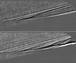
Time-averaged schlieren was used to assess the accuracy of the computed base flow relative to the experiments and study the overall reattachment trends of the bubble. Figure 4 shows a composite image of the experimental schlieren for the overall bubble, with computed density isolines overlaid on top. The isolines are closely spaced in regions of high density gradient. Excellent agreement can be seen between the measured and computed shear-layer locations based on this comparison. Additionally, the position of the separation shock and the height of the reattached boundary layer also agree well with the computational results.

Figure 4. Time-averaged schlieren of the separation bubble with computed density isolines overlaid on top. Experimental results at  $Re_\infty =12.4\times 10^6\ {\rm m}^{-1}$, computational results at $Re_\infty =12.7\times 10^6\ {\rm m}^{-1}$. Flow is from left to right, scale is in millimetres, with the origin at the compression corner.
The time-averaged schlieren imagery was also utilized to estimate the reattachment locations from the experiments at three unit Reynolds numbers. Higher  $Re_\infty$ values could not be run with the large sapphire windows due to pressure limitations, so full-scale schlieren could not be acquired for them. An edge-finding algorithm was applied to the time-averaged schlieren, with the results displayed in figure 5. The images have been rotated such that the reattached boundary layer is horizontal. A red trend line is overlaid on the boundary layer for each case. The reattachment point for the bubble was estimated by the location where the boundary layer curves away from the trend line (similar to the method used by Butler & Laurence Reference Butler and Laurence2021), and is marked in each image with a red dot. To find accurate locations where this curvature occurs, the pixel intensity profile was extracted along the trend line and scaled (dashed coloured lines in figure 6a). An error function fit was then applied to that profile (solid colored lines in figure 6a). Reattachment was determined by where this fit crosses 0.95 (solid black line in figure 6a). For the runs analysed, the flow generally reattached between 75 and 95 mm downstream of the compression corner, depending on freestream Reynolds number (figure 6b). Error bars were added to show variations within 5 % of the estimated reattachment point. In general, the reattachment point moved downstream with increasing unit Reynolds number, which is expected for a laminar separation bubble (Becker & Korycinski Reference Becker and Korycinski1956). The computed reattachment point, determined by where the numerical zero-velocity contour intersects the surface, is also included in figure 6(b). This computed position agrees within 5 % of the estimated experimental results.

Figure 5. Processed time-averaged schlieren used to estimate the bubble reattachment locations. Trend lines along which pixel intensity profiles were extracted are shown in red, with the estimated reattachment location marked by a red dot. Flow is primarily from left to right, scale is in millimetres. Here, (a)  $Re_\infty =8.0\times 10^6\ {\rm m}^{-1}$, (b) $Re_\infty =10.3\times 10^6\ {\rm m}^{-1}$ and (c) $Re_\infty =12.4\times 10^6\ {\rm m}^{-1}$.

Figure 6. Data used to compute estimated reattachment. (a) Scaled intensity profiles along the linear fit of the reattached boundary layer (coloured dashed lines) and their error-function approximations (coloured solid lines). The reattachment point locations were determined by where the error function fits cross 0.95 (solid black line). (b) Measured and computed reattachment point locations downstream of the nosetip. Error bars of 5 % are included, within which the computed case falls. Laminar reattachment locations are extrapolated for higher  $Re_\infty$ with a dashed yellow line.
A linear extrapolation was added to figure 6(b) to estimate where reattachment might occur for the higher unit Reynolds number cases run in this study. Note that this extrapolation assumes that the laminar trend holds; if transition begins along the bubble, then this trend should reverse (Becker & Korycinski Reference Becker and Korycinski1956). Therefore, this line represents the downstream-most expected reattachment positions for these higher unit Reynolds numbers. Based on this plot, the reattachment point should be upstream of the end of the flare, located 104.8 mm from the compression corner, for all unit Reynolds numbers tested.
Compared to previous 10 $^{\circ }$ flare results that had estimated reattachment locations between 57 and 77 mm downstream of the compression corner (Benitez Reference Benitez2021), the bubble generated with the 12 $^{\circ }$ flare reattached farther downstream for similar unit Reynolds numbers. With both flare angles, the flow was generally laminar at both separation and reattachment. The trend with $Re_\infty$ was therefore also the same, with higher $Re_\infty$ corresponding to the reattachment point occurring farther downstream.
4.2. Instability measurements
PCB, Kulite and high-speed schlieren measurements were utilized to study the instabilities both upstream and downstream of reattachment.
Two clear instabilities were visible in the surface pressure fluctuation power spectra along the flare. The second (Mack) mode (Mack Reference Mack1969) appeared to have a peak between 200 and 250 kHz, depending on the unit Reynolds number. The shear-layer instability (Benitez et al. Reference Benitez, Jewell, Schneider and Esquieu2020) peaked between 90 and 110 kHz depending on the streamwise position. Both instabilities were broad, spanning up to 100 kHz, and have been observed previously on the 10 $^{\circ }$ flare with a sharp nosetip under Mach-6 quiet flow with similar peak frequencies.
Figure 7 plots power spectral densities (PSDs) of three PCB sensors located along the 12 $^{\circ }$ flare. The axial locations given are relative to the compression corner. One sensor is upstream of reattachment, one is near reattachment, and the third is downstream of it. All three sensors contain clear frequency peaks for the two instabilities. The second mode (seen spanning 190–290 kHz) increases in amplitude and peak frequency with increasing unit Reynolds number, while the shear-layer instability (found between 50 and 150 kHz) only increases in amplitude while maintaining its peak frequency.

Figure 7. PCB PSDs for three sensor locations along the 12 $^{\circ }$ flare, plotted for freestream unit Reynolds numbers between $8.15\times 10^6\ {\rm m}^{-1}$ and $14.3\times 10^6\ {\rm m}^{-1}$. Locations are (a) 44 mm, (b) 88 mm and (c) 100 mm downstream of the compression corner.
At most stations, the shear-layer instability has a greater amplitude than the second mode, which differs from the 10 $^{\circ }$ flare results (see figure 8, replotted from Benitez et al. Reference Benitez, Jewell, Schneider and Esquieu2020) but is similar to what Butler & Laurence (Reference Butler and Laurence2022) observed on a cone-flare model for larger flare angles. Additionally, downstream of reattachment, the spectra start to broaden at higher Reynolds numbers, with increasing energy in higher frequencies. This spectral broadening is generally a sign of the onset of boundary-layer transition. At the highest three unit Reynolds numbers, turbulent spots appear in the data for the downstream-most sensors, providing additional evidence that the boundary layer is beginning to transition.

Figure 8. PCB PSDs for three sensor locations along the 10 $^{\circ }$ flare, plotted for freestream unit Reynolds numbers between $6.6\times 10^6\ {\rm m}^{-1}$ and $12.0\times 10^6\ {\rm m}^{-1}$, the maximum quiet Reynolds number at the time (Benitez et al. Reference Benitez, Jewell, Schneider and Esquieu2020). Locations are (a) 80 mm, (b) 105 mm and (c) 117 mm downstream of the compression corner.
PSDs and coherences are plotted for all PCBs along the 12 $^{\circ }$ flare for the highest unit Reynolds number case in figure 9. When holding the freestream unit Reynolds number constant while moving downstream, both the shear-layer instability and the second mode increase in amplitude. The shear-layer instability also increases in peak frequency for the downstream-most sensors (near and downstream of reattachment). This trend is similar to what was observed for the 10 $^{\circ }$ flare with some exceptions. Figure 10 plots the PSDs for both the 10 $^{\circ }$ and 12 $^{\circ }$ flares at the same unit Reynolds number. With the smaller flare angle, the shear-layer instability (between 50 and 150 kHz) tended to stabilize in amplitude and flatten or even break down into two lower-amplitude peaks by the downstream-most sensor. For the larger flare angle, however, the two-peak break never occurs, and instead the instability continues to amplify moving downstream. Additionally, the second-mode peaks for the 10 $^{\circ }$ flare have greater amplitudes than for the 12 $^{\circ }$ flare. This difference is likely due to the longer length of the reattached boundary layer for the smaller flare angle; the second mode is generally neutrally stable as it traverses the shear layer, and begins to amplify again only near reattachment (Balakumar et al. Reference Balakumar, Zhao and Atkins2005).

Figure 9. (a) PCB PSDs and (b) adjacent PCB coherences for the 12 $^{\circ }$ flare, $Re_\infty =14.3\times 10^6\ {\rm m}^{-1}$.

Figure 10. PCB PSDs for the (a) 10 $^{\circ }$ and (b) 12 $^{\circ }$ flares, $Re_\infty =11.5\times 10^6\ {\rm m}^{-1}$.
The coherence values for consecutive sensors over both flare angles for both instability bands generally remain below 0.4 until reattachment approaches (between 57 and 77 mm from the compression corner for the 10 $^{\circ }$ flare, between 75 and 95 mm for the 12 $^{\circ }$ one). As the shear layer moves closer to the surface, the values increase, indicating significant coherence between adjacent sensors. These high coherence values are indicative of travelling wave packets that convect downstream in the shear layer and the reattached boundary layer. Based on high-speed schlieren imagery, these waves traverse the shear layer off the surface upstream of reattachment, resulting in lower surface pressure fluctuation coherence values prior to that point. The coherence results for the 12 $^{\circ }$ flare are similar to those for the 10 $^{\circ }$ one (see Benitez et al. Reference Benitez, Jewell, Schneider and Esquieu2020).
The computed surface pressure N-factors are compared to the measured PCB spectra for the same conditions in figure 11. The linear computed results were scaled such that the most amplified computed peak at 225 kHz (in this case, with wavenumber  $m=10$) located 20 mm downstream of the compression corner aligned with the measured PCB PSD of the same frequency at the same axial position. That scaling factor was held constant moving downstream to compare how the computed and measured spectra amplify. The linear stability results showed two primary peaks, with one centred around 100 kHz, and the other centred around 225 kHz. These computed peak frequencies correspond nearly exactly with the shear-layer and second-mode instability peaks from the experiments at all sensor stations. Good agreement was also seen between the computed and measured amplification rates, with the peak values for both the shear-layer instability and the second mode mostly coinciding with the measured PCB results. Figure 12 plots the integrated PCB amplitudes, integrated between 80 and 120 kHz for the shear-layer instability (listed under 100 kHz in the legend), and between 205 and 245 kHz for the second mode (225 kHz in the legend), along with the computed surface pressure N-factors. The relative scales for the experimental and computational data were set to be equal to the upstream-most data points coinciding between the two datasets. As seen in the previous plots, the computed N-factors agree well with the measured surface pressure fluctuations along the flare, with the computed results only slightly overestimating the experimental amplitudes.

Figure 11. Stability analysis comparisons with PCB spectra, 12 $^{\circ }$ flare, $Re_\infty =12.6\times 10^6\ {\rm m}^{-1}$. Locations are (a) 20 mm, (b) 44 mm, (c) 69 mm, (d) 88 mm, (e) 94 mm and (f) 100 mm downstream of the compression corner.

Figure 12. An N-factor comparison with integrated PCB amplitudes. PCB results were integrated between 80 and 120 kHz for the 100 kHz data, and between 205 and 245 kHz for the 225 kHz data. Computed N-factors were for  $m=10$.
The SPOD analysis was performed on the high-speed schlieren for the  $Re_\infty =12.7\times 10^6\ {\rm m}^{-1}$ case. This was the highest quiet unit Reynolds number run with the large windows capable of capturing the reattachment point. The camera was oriented to be parallel to the flare, and configured to run with frame rate 875,000 frames per second. Figure 13 plots the relative SPOD energy for each mode as a function of frequency, normalized by the total energy. Due to the pulsed-burst capture method of the light source and camera, the primary SPOD mode tended to correspond to a whole-image blinking that is non-physical; therefore, only modes 2 and above are shown. The SPOD energy plot for mode 2 (plotted in red) mimics what was observed in the surface pressure fluctuation spectra, and looks very similar to the PSDs in figure 10(b). In particular, the shear-layer instability and second mode result in broad peaks centred on 100 kHz and 230 kHz, respectively. Two sharp peaks are also visible at 10 and 34 kHz, which appear to correspond to additional unsteadiness in the flow as opposed to noise.

Figure 13. SPOD relative mode energy as a function of frequency, 12 $^{\circ }$ flare, $Re_\infty =12.7\times 10^6\ {\rm m}^{-1}$.
Disturbance frequency mode shapes of several frequencies from the SPOD analysis are displayed in figure 14. All SPOD images use the same intensity scale. The separation bubble edge, determined by the zero-velocity streamline from the computations, is plotted as a dashed green line in each image, and the boundary-layer edge is displayed as a solid yellow line. Four distinct mode shapes were observed in the shear layer and/or reattached boundary layer along the flare. At 10 kHz, a ‘flapping’ mode was seen, which could also be observed visually in the unprocessed schlieren. This mode appears primarily downstream of reattachment, and tended to correspond with broad, coherent motion of the boundary layer itself. At 34 kHz, approximately 10 mm wide fluctuations can be observed in the shear layer, which begin to dampen downstream of reattachment. Narrow peaks at the same frequency were also observed in the PCB and Kulite spectra (e.g. in figure 10b), but have not previously been a focus of study. At 98 kHz, the shear-layer instability can be observed clearly. It begins amplifying along the shear layer, and continues to amplify downstream of reattachment. Finally, the second mode is seen at 234 kHz. Like the shear-layer instability, it is present in both the shear layer and downstream of reattachment.

Figure 14. SPOD mode shapes near reattachment for the 12 $^{\circ }$ flare at $Re_\infty =12.7\times 10^6\ {\rm m}^{-1}$. The computed bubble edge is denoted by the dashed green line, while the computed boundary-layer edge is displayed as a solid yellow line. Flow is primarily from left to right, and the intensity scale is the same between images. Frequencies are (a) 10 kHz, (b) 34 kHz, (c) 52 kHz, (d) 98 kHz, (e) 178 kHz and (f) 234 kHz.
An additional observation from the SPOD analysis is that the lower-frequency fluctuations and the shear-layer and second-mode instabilities were well isolated in frequency space, supporting the notion that they are distinct from each other. The lack of any strong, coherent disturbances in the bands between these fluctuations is apparent in figures 14(c) and 14(e). No coherent fluctuations were observed above 270 kHz. This contrasts with SPOD results for turbulent boundary layers, where coherent content can be extracted across a broad spectrum of frequencies continuously (Hill et al. Reference Hill, Borg, Benitez and Reeder2023).
Numerical schlieren mode shapes at corresponding frequencies are displayed in figure 15. The separation bubble and boundary-layer edge are plotted in the same way as in figure 14. These images are qualitative, as the mode shapes are determined independently for each frequency using a linear solver, so the relative amplitudes of the numerical disturbance frequency modes cannot be compared directly as they can for the experimental SPOD. Therefore, the intensity scales vary between the different frequency modes to highlight the shape of each disturbance. This qualitative nature is exemplified in the lack of coherent fluctuations at 178 kHz in the experiments, due to the low amplitude of this mode (figure 14e), but in the computations, the mode shape can be seen clearly due to the manual scaling. Good agreement in wavelength, shape and location can be observed between the mode shapes obtained from the experimental SPOD images and those computed with the numerical schlieren.

Figure 15. Numerical schlieren mode shapes near reattachment for the 12 $^{\circ }$ flare at $Re_\infty =12.6\times 10^6\ {\rm m}^{-1}$. The computed separation bubble edge is denoted by the dashed green line, while the computed boundary-layer edge is displayed as a solid yellow line. Flow is primarily from left to right, and the intensity scale is adjusted independently for each image to better visualize the mode shape. Frequencies are (a) 10 kHz, (b) 34 kHz, (c) 52 kHz, (d) 98 kHz, (e) 178 kHz and (f) 234 kHz.
The shear-layer and second-mode instabilities were also observed more directly in the high-speed schlieren. Figure 16(a) shows disturbances propagating in the shear and boundary layer. Each of the six frames plots a vertical column of pixels over time with the axial position of the pixel line located directly above a PCB sensor installed along the flare. The associated PCB signals and power spectra are plotted in figure 17. In figure 17(a), the PCB time series are offset artificially for clarity, with the upstream-most sensor (located 57 mm downstream of the corner) at the top, and the downstream-most one (100 mm downstream of the corner) at the bottom; however, the signals themselves are all zero-centred in reality. The time period selected had several wave packets, but contained no significant spectral broadening or turbulent spots. By plotting the schlieren pixel column as a function of time, the variation in frequencies of the different shear- and boundary-layer disturbances can be observed clearly. The corresponding PSDs for all heights off the model surface are displayed in figure 16(b). Note that the shear layer is mostly above the available view for the first station. A small, 35 kHz fluctuation is present at most of the stations, though most dominantly in the second and third (69 and 82 mm downstream of the corner, respectively). Additional energy can be seen at 80–120 kHz and 210–250 kHz, corresponding to the shear-layer instability and the second mode, respectively. The peak at 260 kHz that spans the entire window height is believed to be either laser noise or an off-axis instability, since it was evenly distributed across the entire view without aligning to any aerodynamic structure.

Figure 16. (a) Mean-subtracted schlieren time series and (b) schlieren PSDs, 12 $^{\circ }$ flare, $Re_\infty =12.7\times 10^6\ {\rm m}^{-1}$. Each station corresponds to a streamwise position of a PCB sensor, located at 57, 69, 82, 88, 94 and 100 mm downstream of the compression corner. The corresponding PCB data are plotted in figure 17.

Figure 17. (a) PCB time series and (b) PCB PSDs, 12 $^{\circ }$ flare, $Re_\infty =12.7\times 10^6\ {\rm m}^{-1}$. The corresponding schlieren data are displayed in figure 16.
To obtain a better understanding of the spatial distribution of each disturbance, integrated PSD values were plotted from the schlieren imagery in figure 18. The colour scale is the same in all five images. The model surface is plotted as white solid lines, while the same reference lines for the boundary-layer edge and the bubble edge are drawn in yellow and green, respectively. Energy from all three frequency bands (centred around 35 kHz, 100 kHz and 230 kHz) is present in the upper regions of both the shear layer and the reattached boundary layer, and is generally absent in the bands between and after them. The second mode and shear-layer instability also appear to amplify moving downstream in the reattached boundary layer. The 35 kHz fluctuation, however, appears to dampen out, starting at approximately 85 mm downstream of the compression corner. Interestingly, the shear-layer instability, between 80 and 120 kHz, has two primary peak locations, while the 35 kHz fluctuations seem to follow a single primary path line. The second mode (between 210 and 250 kHz) begins with a single path but adds a second peak location near and downstream of reattachment.

Figure 18. Integrated PSDs across the shear and boundary layer, 12 $^{\circ }$ flare, $Re_\infty =12.7\times 10^6\ {\rm m}^{-1}$. The white dashed line represents reattachment, while the yellow curve represents the estimated shear/boundary-layer edge. Frequencies are (a) 25–45 kHz, (b) 80–120 kHz, (c) 150–190 kHz, (d) 210–250 kHz and (e) 270–310 kHz.
The dual-peak distribution of the shear-layer instability agrees with the SPOD mode shape at 98 kHz displayed in figure 14(d). In that figure, fluctuations can be seen in two regions that are 180 $^{\circ }$ out of phase with each other, with one located directly above the shear- and boundary-layer edges, and the other located approximately 0.3 mm above that. Integrating these fluctuations would result in maxima along the two regions, with a minimum between them where the phase of the fluctuations change. The integrated spectral density in figure 18(b) follows this expected pattern.
Band-pass filtering the schlieren and PCB signals allowed for a direct comparison of wave packets measured simultaneously with two separate techniques. Figure 19 plots the results for the shear-layer and second-mode instabilities from the data shown in figure 16(a). In both cases, a sample wave packet for the respective instability is highlighted, with black lines denoting the notional beginning and end of that packet. The PCB time series in figures 19(c) and 19(d) are offset for clarity (similar to figure 17a). The wave packets tended to appear in the schlieren data prior to in the PCB data, implying a slight downward wall-normal velocity component for the waves. This finding agrees with previous results comparing FLDI and PCB measurements with the 10 $^{\circ }$ flare (Benitez Reference Benitez2021). Band-passing the same signals between 25 and 45 kHz to observe the 35 kHz instability resulted in a clear wave packet in the third to fifth schlieren stations (82, 88 and 94 mm from the corner), as displayed in figure 20. However, no obvious correlates were found in the band-passed PCB signals around the same time.

Figure 19. (a,b) Band-passed filtered schlieren and (c,d) PCB data at the same axial locations, 12 $^{\circ }$ flare, $Re_\infty =12.7\times 10^6\ {\rm m}^{-1}$. Frequency bands defined for (a,c) the shear layer at 80–120 kHz, and (b,d) second mode at 210–250 kHz instabilities.

Figure 20. (a) Band-passed filtered schlieren and (b) PCB data at the same axial locations, 12 $^{\circ }$ flare, $Re_\infty =12.7\times 10^6\ {\rm m}^{-1}$. Frequency band defined for the 35 kHz instability between 25 and 45 kHz.
Cross-correlating the schlieren signal with the PCBs provides more information about the wave packet coherency and velocities. The cross-correlations and peak lag times for the shear-layer and second-mode instabilities are shown in figure 21. Schlieren data were extracted from 1.24 and 2.16 mm off-surface for the 80–120 kHz and 210–250 kHz cases, respectively, at 94 mm downstream of the compression corner. A clear peak in the envelope of the cross-correlation is present for both instabilities. With peak amplitudes above 0.45 and cross-correlation values below 0.20 away from the peak, the schlieren and PCB data show excellent agreement in these two bands. By plotting axial displacement as a function of lag time at maximum cross-correlation, the disturbance velocity for both instabilities may be estimated downstream of reattachment. For this case, the shear layer instability has a disturbance velocity of approximately  $768\ {\rm m}\ {\rm s}^{-1}$ when cross-correlating PCB and schlieren results. If each of the schlieren results is cross-correlated with the schlieren time series from 94 mm downstream, then the velocity is estimated at $743\ {\rm m}\ {\rm s}^{-1}$, while if only the PCBs are cross-correlated, then the result is $791\ {\rm m}\ {\rm s}^{-1}$. These velocity estimates are all within 7 % of each other. For the second mode, the schlieren–PCB cross-correlation results in a disturbance velocity $753\ {\rm m}\ {\rm s}^{-1}$, while the schlieren–schlieren velocity is $782\ {\rm m}\ {\rm s}^{-1}$ and the PCB–PCB velocity is $780\ {\rm m}\ {\rm s}^{-1}$; all velocity estimates are within 4 %. Both frequency bands therefore have similar velocity estimates of between 743 and $791\ {\rm m}\ {\rm s}^{-1}$, corresponding to between 87 % and 92 % of the freestream velocity. These results differ from the 10 $^{\circ }$ flare case, which consistently saw a significantly faster disturbance speed for the shear-layer instability than the second mode (Benitez Reference Benitez2021).

Figure 21. Schlieren and PCB signal cross-correlation for the shear-layer and second-mode instabilities, 12 $^{\circ }$ flare, $Re_\infty =12.7\times 10^6\ {\rm m}^{-1}$. The schlieren data were taken from 94 mm downstream of the compression corner and cross-correlated with PCB data from each axial station. The vertical axes for (b,d) display displacement from this 94 mm position. The black dashed line represents the estimated reattachment location. (a) Schlieren–PCB cross-correlation, band-passed between 80 and 120 kHz. (b) Lag times at maximum cross-correlation, band-passed between 80 and 120 kHz. (c) Schlieren–PCB cross-correlation, band-passed between 210 and 250 kHz. (d) Lag times at maximum cross-correlation, band-passed between 210 and 250 kHz.
The cross-correlations of the 35 kHz fluctuation schlieren and PCB data are plotted in figure 22(a). The results contain relatively high, fluctuating cross-correlation values that do not coalesce into a single peak that can be tracked in time. The lag times at maximum cross-correlation also appear scattered (figure 22b). The high correlation values are likely due to the narrow frequency range of the band-passed data (just 20 kHz, selected to exclude other low-frequency disturbances from the analysis). The scattered peak lag times and lack of any clear dominant peak likely mean the schlieren and PCB data generally do not contain the same correlated wave packets despite both measurement techniques observing a 35 kHz peak. The PCB–PCB peak lag times were similarly scattered. However, the schlieren–schlieren lag times do appear linear upstream of reattachment, with an estimated disturbance velocity  $844\ {\rm m}\ {\rm s}^{-1}$ (about 99 % of the freestream velocity). This coherence within the schlieren data agrees with the visible wave packets seen in figure 20.

Figure 22. Schlieren and PCB signal cross-correlations for the 35 kHz fluctuation, 12 $^{\circ }$ flare, $Re_\infty =12.7\times 10^6\ {\rm m}^{-1}$. The schlieren data were taken from 69 mm downstream of the compression corner and cross-correlated with PCB data from each axial station. The vertical axis for (b) displays displacement from this 69 mm position. The black dashed line represents the estimated reattachment location. (a) Schlieren–PCB cross-correlation and (b) lag times at maximum cross-correlation, band-passed between 25 and 45 kHz.
Bicoherence analysis can be used to determine if any nonlinear phase-locking is present in the time series data prior to breakdown. The bicoherences for one of the downstream-most PCBs in each of the 10 $^{\circ }$ and 12 $^{\circ }$ flares are plotted in figure 23, with the surface pressure fluctuation PSD displayed above it for reference. The conditions selected for the 12 $^{\circ }$ flare angle were set to match the freestream unit Reynolds number for the 10 $^{\circ }$ flare result. Both cases use 0.1 s of data that do not contain any turbulent spots. Two primary peaks can be seen at very similar frequency pairs for both flare angles. The first peak, at $(\,f_1,f_2)=(215,100)$, corresponds to a nonlinear interaction between the shear-layer instability (which peaks at 100 kHz for both flares) and the second mode (which peaks at approximately 215 kHz at this Reynolds number). The second peak occurs at $(\,f_1,f_2)=(215,215)$, which corresponds to the first harmonic of the second mode. The stronger bicoherence for the 10 $^{\circ }$ flare is likely due to the longer length of the reattached boundary layer by the measured position, due to the upstream reattachment point for the lower flare angle; the bicoherence values were significantly lower 12 mm upstream on the 10 $^{\circ }$ flare, but with peaks at the same two frequency pairs.

Figure 23. PCB PSDs and bicoherence for the 10 $^{\circ }$ and 12 $^{\circ }$ flares, $Re_\infty =11.5\times 10^6\ {\rm m}^{-1}$. Bicoherence significance threshold $b^2_{95}=0.0075$. (a) 10 $^{\circ }$ flare, 105 mm downstream of the compression corner. (b) 12 $^{\circ }$ flare, 100 mm downstream of the compression corner.
4.3. Breakdown to turbulent spots
Prior global instability analysis of the cone-cylinder-flare geometry at Mach 6 and  $Re_\infty =11.5\times 10^6\ {\rm m}^{-1}$ by Paredes et al. (Reference Paredes, Scholten, Choudhari, Li, Benitez and Jewell2022) and Li et al. (Reference Li, Choudhari, Paredes and Scholten2022) indicated that the growth rate of the separation region initially becomes unstable for a $9^\circ$ flare angle, but that at $12^\circ$ flare angle, the flow becomes highly globally unstable. A similar global analysis for this geometry and conditions has been performed. The characteristics of the dominant families of global instabilities are shown in figure 24, with the variation in the corresponding values of the frequency and temporal growth rate as a function of the azimuthal wavenumber shown in figures 24(a) and 24(b), respectively. The largest growth rate is observed for a stationary mode at $m=26$, shown by the ‘mode 1’ curve. At lower wavenumbers, between $m=14$ and $m=22$, the leading two stationary modes become a travelling pair of modes. Additional mode families are shown by the modes 3 and 4 curves for a pair of travelling modes, and the mode 5 curve for another mode that becomes the travelling pair of mode 2 for $m<12$. The overall significance of these global modes is beyond the scope of the linear stability analysis considered herein. However, the general agreement between the predicted spectra of the convective instability modes and the measured spectra of the surface pressure fluctuations suggests that the global modes may not exert a major influence on the overall evolution of the convective modes. For more details on the modal topology observed for this geometry at similar conditions, the reader is directed to Li et al. (Reference Li, Choudhari, Paredes and Scholten2022). Nevertheless, the large temporal growth rate present for modes 1–5 indicates a greater likelihood that this configuration may lead to turbulent spot creation and breakdown.

Figure 24. Frequency and growth rate characteristics of the dominant global modes as a function of azimuthal wavenumber, 12 $^{\circ }$ flare, $Re_\infty =12.6\times 10^6\ {\rm m}^{-1}$. (a) Global mode frequency. (b) Temporal growth rate.
Indeed, naturally generated turbulent spots were observed in the surface pressure data of the downstream-most PCB sensors for the highest freestream unit Reynolds numbers tested. Figure 25 plots PCB time series for six sensors located along the main sensor ray at  $Re_\infty =14.3\times 10^6\ {\rm m}^{-1}$. The associated PSDs for these data are shown in figure 9(a). In the time series, sharp, high-amplitude spikes start to appear at approximately 88 mm downstream of the compression corner. These spikes increase in number and amplitude moving downstream. The frequency content of the spikes was observed to be broadband with high levels of high-frequency content common to turbulence. Therefore, these spikes are believed to be turbulent spots present in the reattached boundary layer.

Figure 25. Pressure fluctuation time series for six streamwise stations along the 12 $^{\circ }$ flare, $Re_\infty =14.3\times 10^6\ {\rm m}^{-1}$. (a) Time series. (b) Enhanced view of a single turbulent spot.
To determine the relative convection velocity of the turbulent spots, the cross-correlation of the data plotted in figure 25(a) was found for adjacent sensors that contained turbulent spots. The results are plotted in figure 26. The cross-correlation peaks, found at lag times between  $7.2\times 10^{-6}$ and $8.4\times 10^{-6}$ s, correspond to velocities between 714 and $833\ {\rm m}\ {\rm s}^{-1}$.

Figure 26. Cross-correlation between adjacent sensors with turbulent spots, 12 $^{\circ }$ flare, $Re_\infty =14.3\times 10^6\ {\rm m}^{-1}$.
A bicoherence analysis was conducted on these data to determine any nonlinear phase-locking between disturbances as the turbulent spots form (figure 27). At 57 mm downstream of the corner (located upstream of reattachment, which is likely downstream of 90 mm at these conditions), the bicoherence is generally low. By 69 mm, a very slight peak at  $(\,f_1,f_2)=(100,250)$ (circled in red) begins to emerge, corresponding to the nonlinear interaction between the shear-layer instability and the second mode. By 82 mm downstream, a strong peak can be seen at these frequencies (again circled in red). One station later, 88 mm downstream of the corner, very high, broadband bicoherence is measured, which is commonly measured when turbulence is present. This strong, broad coherence persists in the final two PCBs downstream.

Figure 27. Bicoherence plots for PCBs at six streamwise stations along the 12 $^{\circ }$ flare, $Re_\infty =14.3\times 10^6\ {\rm m}^{-1}$. The bicoherence significance threshold is $b^2_{95}=0.0075$. Locations are (a) 57 mm, (b) 69 mm, (c) 82 mm, (d) 88 mm, (e) 94 mm and (f) 100 mm downstream of the compression corner.
Continuous-wavelet transform (CWT) scalograms were generated to look at the instantaneous spectra for relevant sensors. Figure 28 displays CWT scalograms for four of the PCBs located the farthest downstream along the 12 $^{\circ }$ flare. The PCB time traces for the same sensors are plotted in figure 29, including the raw pressure fluctuation values as well as the shear-layer and second-mode instability band-passed values. For the sensor located 82 mm downstream of the compression corner, two distinct bands can be observed in the CWT: a 50–150 kHz band where the shear-layer instability resides, and a 190–290 kHz band for the second mode. Moving downstream, wave packets from the shear-layer instability band can be observed clearly to amplify and broaden into the two turbulent spots visible at approximate times 1.2045 and 1.2048 s. From these data, it appears that the shear-layer instability is the source for these turbulent spots. This result, combined with the nonlinear interaction of the shear-layer and second-mode instabilities, implies that the shear-layer instability can be significant to the onset of transition in hypersonic separated flows.

Figure 28. CWT scalograms of the PCBs along the 12 $^{\circ }$ flare highlighting turbulent spot generation from shear-layer instability wave packets for four sensor locations, $Re_\infty =14.3\times 10^6\ {\rm m}^{-1}$. Locations are (a) 82 mm, (b) 88 mm, (c) 94 mm and (d) 100 mm downstream of the compression corner.

Figure 29. PCB pressure traces used to generate the CWT scalograms in figure 28, 12 $^{\circ }$ flare, $Re_\infty =14.3\times 10^6\ {\rm m}^{-1}$. (a) Overall time series data. (b) Time series data band-passed between 80 and 120 kHz (corresponding to the shear-layer instability frequencies). (c) Time series data band-passed between 210 and 250 kHz (corresponding to the second-mode instability frequencies).
Unfortunately, due to the burst-mode capture method of the camera and the low intermittency of the flow, turbulent spots were not captured in the high-speed schlieren at frame rates sufficient to do spectral analysis. However, runs were made at the maximum continuous capture rate (100 kHz) that did include turbulent spots. The supplementary movie available at https://doi.org/10.1017/jfm.2023.533 shows the amplification and breakdown of one such spot at  $Re_\infty =12.3\times 10^6\ {\rm m}^{-1}$. Schlieren time series at six axial positions (57, 69, 82, 88, 94 and 100 mm from the compression corner) from that movie are displayed in figure 30. Turbulent spots occurring at approximately $t=0.966$ s and $t=0.970$ s include significant fluctuations both within the shear or boundary layer and several millimetres above it. These upper fluctuations are likely acoustic noise radiating into the shock layer from the turbulent spots. This noise is not present above the previously shown wave packets (figure 16a).

Figure 30. Mean-subtracted schlieren time series, 12 $^{\circ }$ flare, $Re_\infty =12.3\times 10^6\ {\rm m}^{-1}$. Each station corresponds to a streamwise position of a PCB sensor, located at 57, 69, 82, 88, 94 and 100 mm downstream of the compression corner.
Figure 31 shows the extracted schlieren pixel intensity values at several points along the shear layer (captured at the off-surface heights 4.5 mm, 3.3 mm, 2.3 mm, 2.0 mm, 1.8 mm and 1.5 mm, respectively) and compares them with the PCB signal at the same streamwise locations. Figures 31(a) and 31(b) show that the schlieren clearly measures the same two turbulent spots captured in the pressure sensors near  $t=0.966$ s and $t=0.970$ s. The schlieren fluctuations increase slightly earlier in time than the PCBs, as well as farther upstream, which supports the initiation of the fluctuations being off-surface in the shear layer. Band-passed PCB signals are plotted in figures 31(c) and 31(d) to show when fluctuations associated with the shear-layer instability and the second mode first appear. Similar to the CWT plots shown previously, the shear-layer instability (at approximately 100 kHz) appears first and amplifies into the turbulent spots. The second-mode frequencies (at approximately 230 kHz) are not observable until approximately 94 mm downstream, when the wave packets are breaking down.

Figure 31. Schlieren intensities in the shear layer compared to PCB time series at the same streamwise positions, 12 $^{\circ }$ flare, $Re_\infty =12.3\times 10^6\ {\rm m}^{-1}$. (a) Schlieren intensities in the shear layer. (b) PCB time series at the same axial locations. (c) PCB time series band-passed for the shear-layer instability (between 80 and 120 kHz). (d) PCB time series band-passed for the second mode (between 210 and 250 kHz).
The overall number of turbulent spots and the turbulent intermittency for several runs are plotted as a function of length Reynolds number in figure 32. The reference length for the Reynolds number was set to the axial distance between the sensor at which the data were computed and the compression corner. For the intermittency,  $0$ corresponds to fully laminar flow with no turbulent spots, while $1$ corresponds to fully turbulent flow. To find this value, the PCB data were first high-pass filtered above 300 kHz to focus on the broadband high-frequency rise above the band containing the laminar instabilities. A threshold of 20 Pa was then used with these filtered data. Runs with Reynolds numbers below $0.8\times 10^6$ were conducted, but both spot count and intermittency were zero for those lower Reynolds numbers. In general, turbulent spots were not observed below Reynolds numbers of $1.1\times 10^6$. From that point, the number of spots and turbulent intermittency begin increasing exponentially, as can be seen by the linear trend for each when the non-zero values are plotted on a logarithmic scale (figure 32b); the exponential trend lines plotted in the figure have $R^2$ values 0.57 and 0.75 for the number of spots and intermittency, respectively.

Figure 32. Turbulent spot count and intermittency, 12 $^{\circ }$ flare. (a) Linear scale. (b) Logarithmic scale with exponential trend lines.
No naturally generated turbulent spots occurred with the 10 $^{\circ }$ flare model, but turbulent-spot-like structures were observed with plasma perturbation of the upstream boundary layer. The plasma perturber was used with that geometry to input a broadband, high-amplitude initial disturbance into the boundary layer upstream of the separation bubble. This artificially generated disturbance was pulsed at a 2 kHz rate and resulted in an impulse with a flat frequency response past 5 MHz. The noise spike from the perturber was removed manually from the pressure trace, with the resulting wave packet remaining. This wave packet generated from the disturbance convected downstream in the shear and reattached boundary layers of the 10 $^{\circ }$ flare. The electrodes for the perturber were placed at the downstream end of the cone, which is downstream of the primary region of second-mode amplification, but upstream of the separation point. For more information about the set-up and characterization of this experiment, see Benitez et al. (Reference Benitez, Jewell and Schneider2021).
Figure 33 displays CWT scalograms of three PCB sensors along the 10 $^{\circ }$ flare. The associated pressure time series, as well as the band-passed time series at the shear-layer and second-mode instability frequency bands, are plotted in figure 34. Two wave packets are seen at each station, starting with a sinusoidal signal centred at 100 kHz, 64 mm downstream of the compression corner. This wave packet is in the shear-layer instability band, and broadens in frequency as it convects downstream, so that by 117 mm downstream, the packet resembles a turbulent spot. In the band-passed time series data, the shear-layer instability (associated with the 80–120 kHz band) includes clear wave packets at all stations in the reattached boundary layer, while wave packets in the second-mode band (195–235 kHz for these conditions) do not appear until about 93 mm downstream. These results are similar qualitatively to what has been observed naturally without perturbation with the 12 $^{\circ }$ flare.

Figure 33. CWT scalograms from PCB sensors along the 10 $^{\circ }$ flare with plasma perturbation. Potential turbulent spots are seen evolving from shear-layer instability wave packets across three sensor locations, $Re_\infty =11.6\times 10^6\ {\rm m}^{-1}$. Replotted from Benitez et al. (Reference Benitez, Borg, Paredes, Schneider and Jewell2023). Locations are (a) 80 mm, (b) 93 mm and (c) 117 mm downstream of the compression corner.

Figure 34. PCB pressure traces used to generate the CWT scalograms in figure 33, 10 $^{\circ }$ flare, $Re_\infty =11.6\times 10^6\ {\rm m}^{-1}$. (a) Overall time series data. (b) Time series data band-passed between 80 and 120 kHz. (c) Time series data band-passed between 195 and 235 kHz.
5. Conclusions
A hypersonic wind tunnel study was conducted on a cone-cylinder-flare with a 12 $^{\circ }$ flare angle and a nominally sharp nosetip under low-disturbance flow, with support from a computational linear stability analysis. The estimated reattachment point was found to move downstream with increasing freestream unit Reynolds number. Based on that trend, as well as surface pressure fluctuation spectra, the SBLI separation bubble was determined to be primarily laminar through reattachment. Excellent agreement was seen between the laminar computed base flow and the schlieren images from the experiments. Relative to prior measurements made on a 10 $^{\circ }$ flare, the reattachment point was farther downstream from the compression corner for this 12 $^{\circ }$ flare angle.
Two clear instabilities were observed in both the surface pressure fluctuation and high-speed schlieren measurements: the shear-layer instabilities in the same band as Mack's first mode (50–150 kHz) and the second (Mack) mode instability (190–290 kHz). The frequency bands and amplification rates for both instabilities agreed well with linear stability analysis predictions for convective waves. While similar to instability measurements made with a 10 $^{\circ }$ flare, the shear-layer instability for this larger flare angle differed by being more amplified than the second mode. Global instability analysis showed several unstable families of stationary and travelling three-dimensional modes, but the general agreement between the predicted spectral of the convective instability modes and the measured spectra suggests that the global modes may not exert a major influence on the overall evolution of the convective modes. High-speed schlieren imagery was used in an SPOD analysis for one case run with a very high frame rate (875 kHz). The SPOD relative mode energy agreed exceptionally well with the PCB spectra, clearly showing peaks in the shear-layer and second-mode instability bands. Additional, lower-frequency content at approximately 10 kHz and a sharp peak at 34 kHz were also observed. These two lower-frequency disturbances appear to correspond to aerodynamic phenomena based on the extracted SPOD mode shapes. However, more work is necessary to confirm their role (if any) in transition and bubble stability. Band-passed schlieren data were compared to simultaneous PCB measurements for individual wave packets. High cross-correlation between the two measurement techniques was observed for the shear-layer and second-mode instability bands, with wave packet velocities at approximately 87–92 % of the freestream velocity. However, PCB and schlieren wave packets in the 35 kHz band appeared to be uncorrelated.
For the first time in axisymmetric, low-disturbance hypersonic flow, turbulent spots were generated naturally downstream of a laminar separation bubble. A CWT analysis of the pressure fluctuations revealed that these spots tend to evolve from wave packets in the shear-layer instability frequency band. Due to limitations of the high-speed schlieren instrumentation, lower-speed schlieren was used to capture the turbulent spots; however, these measurements still agreed well with simultaneous PCB data. Bicoherence analysis of the surface pressure data also supports nonlinear phase-locking between the shear-layer and second-mode instabilities. While no naturally occurring turbulent spots were present on the 10 $^{\circ }$ flare, artificially generated disturbances made with a plasma perturber did produce similar turbulent-spot-like structures in the reattached boundary layer. Due to the low-disturbance environment of the test facility (with similar freestream fluctuation levels to flight), it is likely that a similar shear-layer-instability-dominated transition mechanism could occur with a real hypersonic vehicle.
Supplementary movie
Supplementary movie is available at https://doi.org/10.1017/jfm.2023.533.
Acknowledgements
The authors would like to thank Dr A. Berger and J.L. Hill for their insightful conversations. They would also like to thank C. Chinske for transportation of the model.
Funding
A.S. and P.P. are supported by the US Office of Naval Research under award no. N00014-20-1-2261. P.P. is also partially supported by the Hypersonic Technology Project (HTP) under the NASA Aeronautics Research Mission Directorate (ARMD) and by the Air Force Office of Scientific Research (AFOSR) under award no. FA9550-20-1-0023. The computational resources supporting this work were provided by the DoD High Performance Computing Modernization Program and the NASA LaRC K Cluster at the Langley Research Center. J.S.J. and Z.McD. are partially supported by the Air Force Research Laboratory under contract nos FA8650-19-C-2404 and FA8650-20-C-2407.
Declaration of interests
The authors report no conflict of interest.


