2. Governing equations and control parameters

The flow in RB convection is confined between two parallel plates separated by a distance $H$, with gravitational acceleration $g$ acting orthogonally to these plates. We numerically integrate the velocity field $\boldsymbol {u}$ and the temperature field $\theta$ according to the Navier–Stokes equations subject to the Oberbeck–Boussinesq approximation, ignoring potential density anomalies which e.g. occur for water at $4\,^\circ$C. We implement the phase-field method presented by Hester et al. (Reference Hester, Couston, Favier, Burns and Vasil2020) to simulate the melting solid. In this technique, the phase field variable $\phi$ is integrated in time and space, and smoothly transitions from a value of 1 in the solid to a value of 0 in the liquid. The dimensionless governing equations, constrained by the incompressibility condition $\boldsymbol{\nabla} \boldsymbol{\cdot} \boldsymbol {u} = 0$, read

(2.1)\begin{gather} \frac{\partial\boldsymbol{u}}{\partial t}+\boldsymbol{u}\boldsymbol{\cdot}\boldsymbol{\nabla} \boldsymbol{u} ={-}\boldsymbol{\nabla} p + \sqrt{\frac{Pr}{Ra}}\nabla^2 \boldsymbol{u} -\frac{\phi \boldsymbol{u}}{\eta} + \theta \boldsymbol{e}_z, \end{gather}

(2.2)\begin{gather}\frac{\partial\theta}{\partial t}+\boldsymbol{u}\boldsymbol{\cdot}\boldsymbol{\nabla}\theta=\frac{1}{\sqrt{RaPr}} \nabla^2\theta+St\frac{\partial\phi}{\partial t}, \end{gather}

(2.3)\begin{gather}\frac{\partial\phi}{\partial t}=\frac{6}{5StC\sqrt{RaPr}}\left[\nabla^2\phi-\frac{1}{\epsilon^2} \phi(1-\phi)(1-2\phi+C\theta)\right]. \end{gather}

Here, the temperature field $\theta = (T-T_m)/\varDelta$ has been non-dimensionalized using the temperature difference $\varDelta$ between the plates and the equilibrium melting temperature $T_m$, and the velocity field $\boldsymbol {u}$ has been non-dimensionalized with the free-fall velocity $U_{f} = \sqrt {g\beta H {\rm \Delta} }$, where $\beta$ is the thermal expansion coefficient; $\boldsymbol {e}_z$ is the direction of gravity and $\eta$ is the penalty parameter to damp the velocity to zero in the solid phase, which we set equal to the time step, following Favier et al. (Reference Favier, Purseed and Duchemin2019). All lengths have been made non-dimensional with the plate separation $H$. The physical control parameters in the equations are the Rayleigh, Prandtl and Stefan numbers, defined as

(2.4a–c)\begin{equation} Ra=\frac{\beta g {\rm \Delta} H^3}{\nu\kappa} ,\quad Pr=\frac{\nu}{\kappa} ,\quad St=\frac{\mathcal{L}}{c_p{\rm \Delta}} . \end{equation}

Here, $\nu$ is the kinematic viscosity of the liquid, $\kappa$ is the thermal diffusivity (which is assumed to be equal in the solid and the liquid), $g$ is the gravitational acceleration, $c_p$ the specific heat and $\mathcal {L}$ the latent heat; $Pr$ is fixed to $10$, representative of cold water. First, $St$ is fixed to $1$, and the effect of increasing $St$ to somewhat more realistic values (in practical situations) for ice and other phase-change materials will be investigated in § 6.

The applied phase-field model was initially derived based on entropy conservation, which guarantees the thermodynamic consistency, and also satisfies the Gibbs–Thompson relation (Hohenberg & Halperin Reference Hohenberg and Halperin1977; Wang et al. Reference Wang, Sekerka, Wheeler, Murray, Coriell, Braun and McFadden1993; Favier et al. Reference Favier, Purseed and Duchemin2019; Hester et al. Reference Hester, Couston, Favier, Burns and Vasil2020), which is given by

(2.5)\begin{equation} \frac{T -T_m}{\varDelta}= \frac{\varepsilon}{C} \gamma, \end{equation}

where $T$ is the dimensional temperature, $T_m$ the equilibrium melting point, $\gamma$ the local interface curvature and $\varepsilon$ is used to measure the diffuse interface thickness; $\epsilon =\varepsilon /H$ is typically chosen as an empirical value in the phase-field method (Ding, Spelt & Shu Reference Ding, Spelt and Shu2007; Yue, Zhou & Feng Reference Yue, Zhou and Feng2010). Here, we take $\epsilon$ to be equal to the grid spacing in our simulations, following the convergence test in Favier et al. (Reference Favier, Purseed and Duchemin2019). Also, $C$ is the same parameter as appears in (2.3). It controls the dependence of the melting point on the interface curvature. At scales relevant for turbulent convection, we anticipate the Gibbs–Thomson effect to be minimal, because the local curvature is relatively low, and therefore we choose $C=1$ (Hester et al. Reference Hester, Couston, Favier, Burns and Vasil2020). The condition of heat flux balance at the liquid–solid interface is given by the classical Stefan conditions (Woods Reference Woods1992; Worster, Batchelor & Moffatt Reference Worster, Batchelor and Moffatt2000) as

(2.6)\begin{equation} \mathcal{L} v_n = c_p\kappa ( \partial_n T^{(S)}-\partial_n T^{(L)}), \end{equation}

where $v_n$ is the normal velocity of the interface, and the superscripts $(S)$ and $(L)$ represent the solid and liquid phases, respectively. A more detailed discussion of the parameters and the validation of our implementation can be found in Hester et al. (Reference Hester, Couston, Favier, Burns and Vasil2020) and also our own software documentation (Howland Reference Howland2022).

Three-dimensional (3-D) simulations are conducted in a domain with ($L_x,L_y,L_z)=(2,1,1)$, where $L_x$, $L_y$ and $L_z$ are the dimensionless horizontal lengths in the $x$ direction, $y$ direction and the dimensionless vertical length in the $z$ direction, respectively. Two-dimensional (2-D) simulations are conducted in a domain with ($L_x,L_z$) = (2,1). We also ensure that there are enough grid points to capture the turbulent flow. Specifically, for the 3-D case of $Ra=10^9$, we use a uniform mesh of $1536\times 768\times 768$. Besides, a grid independence test has been conducted to ensure that the same final conclusion is obtained when the grid size is either halved or doubled. A list of all simulation cases is shown in table 1.

Table 1. List of all simulation cases. Here, $Ra^0_{eff}$ is the effective $Ra$ defined by the initial liquid layer height.

We impose a fixed temperature $\theta =1$ at the bottom heated plate (below the melt) and $\theta =0$ at the top cooled plate (above the frozen liquid), and no-slip boundary conditions for both plates. Periodic boundary conditions are imposed in horizontal directions. The melting temperature of the solid is set to the same value as the temperature at the top wall $\theta =0$. Initially, we prescribe a flat interface height at $h/H=0.1$, with the velocity field set to $\boldsymbol {u}=0$ everywhere. The temperature field in the liquid is initialized as a linear profile with random fluctuations of maximal amplitude 0.01 to trigger a transition to turbulence. Simulations are performed using the second-order staggered finite difference code AFiD (Verzicco & Orlandi Reference Verzicco and Orlandi1996; van der Poel et al. Reference van der Poel, Ostilla-Mónico, Donners and Verzicco2015a), which has already been extensively validated (Kooij et al. Reference Kooij, Botchev, Frederix, Geurts, Horn, Lohse, van der Poel, Shishkina, Stevens and Verzicco2018) and used to study a wide range of convection problems (van der Poel et al. Reference van der Poel, Ostilla-Mónico, Verzicco, Grossmann and Lohse2015b; Yang, Verzicco & Lohse Reference Yang, Verzicco and Lohse2016; Yang et al. Reference Yang, Chong, Wang, Verzicco, Shishkina and Lohse2020; Wang, Lohse & Shishkina Reference Wang, Lohse and Shishkina2021d). The extension of the AFiD code to include two phases approached with the phase-field method (Cahn–Hilliard equation) was discussed and validated in Liu et al. (Reference Liu, Ng, Chong, Lohse and Verzicco2021).

For studying the evolution of the interface topography, the location of the interface, defined implicitly by $\phi =1/2$, is the key response of the system. Locally, we thus define the dimensionless height of the interface $\xi (x,y,t)=h/H$ by the equation $\phi (x,y,\xi (x,y,t),t)=1/2$. From that, we infer the dimensionless mean height of the fluid layer as

(2.7)\begin{equation} \bar{\xi}(t) = \frac{1}{L_xL_y}\int^{L_y}_0\int^{L_x}_0\xi(x,y,t)\, {\rm d} x\, {\rm d} y. \end{equation}

We denote all horizontally averaged values with an overbar. We can use $\bar {\xi }(t)$ to define the effective Rayleigh number of the fluid layer

(2.8)\begin{equation} Ra_{eff}(t)=\frac{\beta g {\rm \Delta} (\bar{h}(t))^3}{\nu \kappa}= Ra(\bar{\xi}(t))^3 \le Ra.\end{equation}

We also define the (non-dimensionalized) local heat flux ${q}$ at the interface as

(2.9)\begin{equation} {q(x,y,t)}={-}\frac{K (\boldsymbol{\nabla} T\boldsymbol{\cdot} {\boldsymbol{n}})|_{{Z}={h}}}{K {\rm \Delta}/{\bar{h}}} ={-}\bar{\xi}(\boldsymbol{\nabla}\theta\boldsymbol{\cdot}{\boldsymbol{n}})|_{{z}=\xi},\end{equation}

where ${Z}$ and ${z}$ denote the dimensional and dimensionless vertical coordinate, respectively, $K=\alpha \rho C_p$ denotes the thermal conductivity and $C_p$ the specific heat; $\boldsymbol {n}$ denotes the normal direction to the solid–liquid interface, calculated by ${\boldsymbol {n}}=\boldsymbol{\nabla} \phi /|\boldsymbol{\nabla} \phi |$. The time-dependent global Nusselt number is defined as

(2.10)\begin{equation} Nu(t)=\bar{q}(t)={-}\bar{\xi} \overline{(\boldsymbol{\nabla}\theta\boldsymbol{\cdot}{\boldsymbol{n}})}|_{{z}=\xi}. \end{equation}

Note that calculating such a diffusive flux directly at $\phi =0.5$ in a phase-field simulation will result in an erroneously small flux since the temperature gradient is smoothed out by the diffuse interface. It is therefore vital to resolve the conductive sublayer, where normal temperature gradients are uniform, outside the diffuse interface region so that the heat flux can be accurately calculated. We have further validated our interfacial heat flux calculations against the Stefan condition (2.6) to ensure self-consistency.

3. Roughness evolution

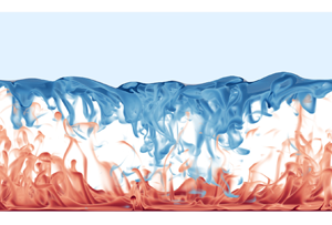
First, we study how the morphology of the initially smooth solid layer above the turbulent convective flow evolves during the melting process. The simulations are run until the layer is completely molten. We present an instantaneous 3-D visualization of the temperature field in figure 1(a). Vertical slices of the temperature field at various times are shown in figure 1(b-d) along with corresponding bottom views of the interface in figure 1(e–g). As seen from these latter figures, the roughness increases as the convective flow intensifies with time. Here, by roughness we refer to the scale of the undulations in the solid–liquid interface. At the early stage, under the influence of convection, the interface evolves from flat to small-scale cellular structures, as shown in figure 1(e). Over time, the cellular structures merge and become larger. The large-scale circulation driven by the convection also grows in scale as time evolves. Furthermore, from figures 1(d) and 1(g), at large $Ra_{eff}$, we do not find isolated cusps above the sinking plumes as in Favier et al. (Reference Favier, Purseed and Duchemin2019) for smaller $Ra_{eff}$, but rather more rough topography from recirculation induced melting. We found that the rough cellular structures exist mainly in the regions associated with descending cold plumes while a smoother surface emerges in the region dominated by the rising hot plumes.

Figure 1. Visualizations of the 3-D numerical simulation at $Ra=10^9$. (a) Instantaneous 3-D temperature field at $t=1200 t_f$. Light blue colour above the flow field represents the solid ice phase $\phi >1/2$. (b–d) Two-dimensional slices of the temperature field at times $400 t_f$, $800 t_f$ and $1200 t_f$, where $t_f=\sqrt {H/g\beta {\rm \Delta} }$ is the free-fall time. (e–g) The contour maps of the solid interface corresponding to the times in (b–d). The topography is found to become rougher as time evolves. Note the different colour code in (g) as compared with (e) and (f), reflecting the roughening of the structure with time.

Apparently, the interface topography changes as $Ra_{eff}$ increases, depending on the rising hot plume region and the descending cold plume region. This also occurs in two dimensions, as highlighted for example by figure 2 for $Ra=10^{11}$: at the early stage, the solid melts locally above the rising hot plume, but less so above the descending cold plume. The unstable descending cold plumes locally generate recirculation flow, as shown in figure 2(a) where $Ra_{eff}=3.1\times 10^8$. While the solid keeps melting and $Ra_{eff}$ increases further, the solid above the cold descending plumes melts faster and becomes rougher than that above the hot rising plumes (see figure 2(b) at $Ra_{eff}=5.3\times 10^{10}$). More unstable cold plumes generate multiple recirculation flows. These turbulent plumes are able to effectively mix their surroundings, thus inducing an increase of the vertical and horizontal heat transport, therefore resulting in more local roughness elements. The early appearance of the recirculation in figure 2(a) was not observed by the previous study of Favier et al. (Reference Favier, Purseed and Duchemin2019). Note that we only have 2-D simulations at high $Ra$. Reiter et al. (Reference Reiter, Shishkina, Lohse and Krug2021) suggest that the higher $Ra$ used in our study is needed to observe the recirculation. The formation of quasi-steady rolls from the normal mode initial condition of Favier et al. (Reference Favier, Purseed and Duchemin2019) leads to coherent interfacial cusps that may also act to inhibit the emergence of such recirculation zones.

Figure 2. (a) Temperature field at $Ra_{eff}=3.1\times 10^8$ of 2-D simulation at $Ra=10^{11}$, with a zoom plot of the interface shape. (b) Temperature field at later time at $Ra_{eff}=5.3\times 10^{10}$, again for 2-D simulation at $Ra=10^{11}$.

4. Roughness amplitude

To quantitatively analyse the topography as time evolves, we first denote the fluctuation terms by a prime, calculated by the local value minus the horizontally averaged value, both for the interface height $\xi$ and heat flux $q$

(4.1a,b)\begin{equation} \xi'(x,y,t)=\xi(x,y,t)-\bar{\xi}(t),\quad q'(x,y,t)=q(x,y,t)-\bar{q}(t),\end{equation}

where $\bar {q} \equiv \bar {\xi } \partial \bar {\theta }/\partial z$. Then we measure the typical amplitude of the interface by the root mean square (r.m.s.) of $\xi '$ as

(4.2)\begin{equation} \xi_{rms}(t)=\sqrt{\overline{(\xi(x,y,t)-\bar{\xi}(t))^2}}= \sqrt{\overline{\xi'(x,y,t)^2}}.\end{equation}

We rescale $\xi _{rms}$ as $\tilde {\xi }_{rms}=\xi _{rms}Ra^{1/3}$ to provide a more general comparison across the different simulations. This is equivalent to non-dimensionalizing the r.m.s. height with the intrinsic length scale $l = (\nu \kappa /g \beta {\rm \Delta} )^{1/3}$ rather than with $H$. Figure 4(a) shows $\tilde {\xi }_{rms}$ as function of the effective Rayleigh number $Ra_{eff}$. The amplitude monotonically increases as $Ra_{eff}$ increases. Deforming cellular structures during merging will cause fluctuations in the results. However, we find that $\tilde {\xi }_{rms}$ depends primarily on the effective Rayleigh number, with a reasonable collapse of the data from all of our simulations, following an approximate scaling of ${Ra_{eff}}^{1/3}$.

We now set out to understand this scaling $\tilde {\xi }_{rms}\sim {Ra_{eff}}^{1/3}$. We begin from the non-dimensionalized Stefan boundary condition (2.6), approximated by only the vertical component of the heat flux

(4.3)\begin{equation} St \frac{\partial \xi}{\partial t}={-}\frac{1}{\sqrt{RaPr}}\frac{\partial\theta}{\partial {z}}= \frac{1}{\sqrt{RaPr}}\frac{q}{\bar{\xi}}, \end{equation}

which relates the melt rate to the local heat flux $q$ using (2.9). Spatial averaging of (4.3) gives

(4.4)\begin{equation} \frac{{\rm d}\bar{\xi}}{{\rm d}t} = \frac{1}{St\sqrt{RaPr}} \frac{{\bar{q}}}{\bar{\xi}}.\end{equation}

By assuming that $\xi '\ll \bar {\xi }$, cancelling out the global balance (4.4) from (4.3) and using (4.1a,b), we obtain

(4.5)\begin{equation} \frac{\partial \xi'}{\partial t} \approx \frac{1}{St\sqrt{RaPr}}\frac{q'}{\bar{\xi}}. \end{equation}

Since $Ra_{eff}$ is solely a function of $t$, as seen in (2.8), we can use the chain rule to transform the time derivative to one with respect to $Ra_{eff}$ and apply (2.8), (4.4) and (4.5), which gives

(4.6)\begin{align} \frac{\partial {\xi}'}{\partial Ra_{eff}} &=\frac{\partial {\xi}'}{\partial t}\frac{\partial t}{\partial \bar{\xi}}\frac{\partial \bar{\xi}}{\partial Ra_{eff}} \approx \left(\frac{1}{St\sqrt{RaPr}}\frac{q'}{\bar{\xi}}\right) \left(St\sqrt{RaPr}\frac{\bar{\xi}}{\bar{q}}\right) \left(\frac{1}{3Ra\overline{\xi}^2} \right)\nonumber\\ & = \frac{q'}{3 \bar{q}} {Ra_{eff}}^{-{2}/{3}}Ra^{-{1}/{3}}. \end{align}

By integrating (4.6), we obtain

(4.7)\begin{equation} \xi'\approx\int\frac{q'}{3 \bar{q}} {Ra_{eff}}^{-{2}/{3}}Ra^{-{1}/{3}}\, {\rm d} Ra_{eff}. \end{equation}

What remains unknown in this expression is the normalized heat flux fluctuation $q'/\bar {q}$, and in particular its dependence on $Ra_{eff}$. Note that in classical turbulent RB convection, it has been found that close to the bottom plate the relative heat transport contributions of the cold descending plume region and the hot rising plumes region are not equal (Zhu et al. Reference Zhu, Mathai, Stevens, Verzicco and Lohse2018). As $Ra$ increases there is a cross-over in these heat flux contributions, and the heat flux from the descending plumes can become dominant at high $Ra$ (Reiter et al. Reference Reiter, Shishkina, Lohse and Krug2021), as there the thermal boundary layer has become very thin.

Here, we also measure the instantaneous interfacial heat flux for regions associated with the descending cold and rising hot plume regions at different $Ra_{eff}$, since $Ra_{eff}$ keeps increasing as the solid melts. Thus we can understand the relation between the roughness and the flow structure underneath. Whereas previous studies (Blass et al. Reference Blass, Verzicco, Lohse, Stevens and Krug2021; Reiter et al. Reference Reiter, Shishkina, Lohse and Krug2021) relied on time averaging to distinguish the separate regions, we must use instantaneous snapshots due to our time-evolving fluid domain. We measure the temperature close to the bottom plate at a distance of $10$ grid points and identify the local temperature maxima, as highlighted in figure 3(b). Note that the exact value of this height does not matter, and our results are robust to changes in this value. The corresponding local heat flux $q$ is plotted in figure 3(c), which reflects the similar behaviour of spatial variation of interface heat flux, leading to the morphology evolution. Note the narrow local peaks in $q$ within the cold plume region, which correspond to the recirculation regions forming secondary cusps at the interface. We then prescribe equally sized areas centred at these peaks such that half of the domain is classified as the ‘rising hot plume’ region. The rest of the domain is classified as the ‘descending cold plume’ as shown on the temperature snapshot of figure 3(a). Five consecutive snapshots are chosen to average the conditionally averaged heat flux.

Figure 3. (a) An illustration of the temperature field and the separated region. The dashed lines represent the edge of the hot rising (in red colour) and cold descending (in blue colour) plume regions. (b) The corresponding temperature distribution as a function of horizontal distance close to the bottom plate at a distance of 10 grid points. The temperature distribution is smoothed by a spatial moving average for each snapshot to avoid instantaneous fluctuations. The red stars represent the measured peak points. Each hot plume region has the same width. (c) The corresponding surface heat flux $q(x)$ calculated at the phase boundary, as defined in (2.9), as a function of horizontal distance. The effective Rayleigh number for this snapshot is $7.5\times 10^{6}$.

Then we plot the conditionally averaged heat flux as a function of $Ra_{eff}$ in figure 4(b). The heat flux contributions remain approximately constant over a wide range from $Ra_{eff}=10^6$ to $Ra_{eff}=10^{10}$. The heat flux fluctuation $q'/\bar {q}$ over the interface can be estimated by the difference between that from the hot rising plume region and that from the cold descending plume region. We do not observe any pronounced dependence on $Ra_{eff}$ so that we can approximate

(4.8)\begin{equation} \frac{q'}{\bar{q}} \approx {\rm const.}\end{equation}

Figure 4. (a) Rescaled topography amplitude $\tilde {\xi }_{rms}=\xi _{rms}Ra^{1/3}$ as a function of the $Ra_{eff}$ (which grows with time) for different global Rayleigh numbers and both 2-D and 3-D simulations. The dashed line shows the $\tilde {\xi }_{rms}\sim Ra_{eff}^{1/3}$ scaling, derived from (4.3) to (4.9). (b) The conditionally averaged heat fluxes averaged over the hot plume region $\bar {q}_h$ and over the cold plume region $\bar {q}_c$ at the interface separately, normalized by the global heat flux at the interface $\bar {q}$. These distinct regions are highlighted in figure 3. Here, the data points are averaged over the five consecutive snapshots around the corresponding $Ra_{eff}$ for 2-D cases. The error bars denote the range of values obtained from these snapshots.

By substituting (4.2) and (4.8) into (4.7), we finally obtain the scaling for the r.m.s. of $\xi$

(4.9)\begin{equation} \tilde{\xi}_{rms}(t)=Ra^{{1}/{3}}\sqrt{\overline{{\xi}'(x,y,t)^2}}\sim Ra_{eff}^{{1}/{3}}, \end{equation}

which is consistent with the results in figure 4(a). This scaling in turn implies that the (dimensional) r.m.s. height is proportional to the mean height, that is

(4.10)\begin{equation} h_{rms}\sim \bar{h}. \end{equation}

This suggests that the large-scale circulation, determined by the layer thickness $\bar {h}$, has the strongest effect on the roughness amplitude. At $Ra_{eff}>10^{10}$, $\tilde {\xi }_{rms}$ shows a deviation from the $Ra_{eff}^{1/3}$ scaling, which could be because of a gradual change of the heat flux distribution in hot and cold plume regions as $Ra$ further increases (similar to what was seen by Reiter et al. (Reference Reiter, Shishkina, Lohse and Krug2021) at $Pr=1$). We could also associate this with the growing importance of the recirculation regions shown in figure 2(b) compared with the large-scale circulation. Such high Rayleigh numbers are not easily achievable with current computational resources but deserve further studies in the future.

5. Roughness wavelength

Another quantity of interest is the typical horizontal scale of the topography. As we shall describe, the circulating flow structures that strongly impact the interface evolution are quite different in 2-D and 3-D simulations, so we choose to analyse them separately.

5.1. Two-dimensional simulations

Focusing mainly on the 2-D simulations, we consider an integral length scale based on the spatial Fourier transform of the interface height $\hat {h}(k,t)$, where non-dimensional $k$ is the wavenumber. Analogous to the typical definition for turbulence, the typical length scale of the topography can then be estimated as $\lambda (t)/H=2\pi /k(t)$, which is defined as

(5.1)\begin{equation} \frac{\lambda(t)}{H}=\frac{\displaystyle \int^{\infty}_0k^{{-}1}| \hat{h}(k,t)|^2\, {\rm d} k}{\displaystyle \int^{\infty}_0|\hat{h}(k,t)|^2\, {\rm d} k}. \end{equation}

The length scale $\lambda (t)/H$ is plotted in figure 5(a) as a function of $\bar {\xi }(t)$ for different $Ra$. As expected, the length scale increases with fluctuations due to the merging cellular structures.

Figure 5. (a) The wavelength $\lambda (t)/H$ of the topography as function of interface height $\bar {\xi }(t)$ for different $Ra$. The dashed line represents $\lambda /H=\bar {\xi }$. For low $Ra$, $\lambda$ is always larger than $\bar {\xi }$, while for high $Ra$, $\lambda$ can be smaller than $\bar {\xi }$, which means that the topography becomes even rougher. (b) Quantity $B$ (defined in (5.3)) as function of $Ra_{eff}$ for different $Ra$. The solid line represents the quadratic fit of our data, and the dashed line represents the fitting curve from Wang et al. (Reference Wang, Verzicco, Lohse and Shishkina2020). (c) The measured convection roll aspect ratio $\varGamma _r$ as a function of $Ra_{eff}$, the lower and upper solid lines represent the lower and upper bounds from the theoretical analyses (5.2) of Wang et al. (Reference Wang, Verzicco, Lohse and Shishkina2020). (d) The measured interface cell aspect ratio $\varGamma _c$ as a function of $Ra_{eff}$, the lower and upper solid lines again represent the lower and upper bounds for interface cells from the theoretical analysis (5.2).

The horizontal scale of the topography is expected to correspond to the wavelength of the underlying convective rolls (Esfahani et al. Reference Esfahani, Hirata, Berti and Calzavarini2018; Favier et al. Reference Favier, Purseed and Duchemin2019). To quantitatively describe the convection rolls, we use the result of Wang et al. (Reference Wang, Verzicco, Lohse and Shishkina2020) for the lower and upper bounds on the aspect ratio of the convective rolls $\varGamma _r$ $=\lambda _r/\bar {h}$, which was derived for smooth plates and no slip boundary conditions. Here, $\lambda _r$ is the wavelength of the convective rolls in classical 2-D RB convection, namely

(5.2)\begin{equation} c\sqrt{B}\le\varGamma_r\le \sqrt{1+2\sqrt{3B}}/\sqrt{1 -2\sqrt{3B}},\end{equation}

with

(5.3)\begin{equation} B\equiv Re^2Pr^2Ra^{{-}1}(\bar{q}-1)^{{-}1},\end{equation}

where $Re$ is the Reynolds number and $c$ is a constant with $c=9$, following Wang et al. (Reference Wang, Verzicco, Lohse and Shishkina2020), and $\bar {q}$ is the averaged heat flux. These upper and lower bounds were derived based on the strain–vorticity balance and a generalized Friedrichs inequality (Wang et al. Reference Wang, Verzicco, Lohse and Shishkina2020). In these 2-D flows, the flow can be assumed as a set of elliptical rolls with a certain range of aspect ratios and the balance between strain and vorticity is determined by the elliptical shape of these rolls. The value of $B$ according to (5.3) is calculated from our simulations and plotted in figure 5(b). It can be fitted by $B = 0.45Ra_{eff}^{-0.38+0.0175\log _{10}(Ra_{eff})}$. The form of this expression comes from a quadratic fit of the data for $\log {B}$ as a function of $\log {Ra_{eff}}$, again as obtained by Wang et al. (Reference Wang, Verzicco, Lohse and Shishkina2020) for smooth walls. In figure 5(c), we plot the convective roll aspect ratio $\varGamma _r$ as function of $Ra_{eff}$ and the upper and lower bounds based on (5.2). As expected, $\varGamma _r$ lies in between them, especially for high $Ra_{eff}$. At low $Ra_{eff}$, disagreements arise since the rough topography is more closely coupled to the convective roll structure, compared with the smooth case in Wang et al. (Reference Wang, Verzicco, Lohse and Shishkina2020), as highlighted by figure 2(a). This can cause smaller aspect ratio rolls to ‘lock-in’ to the shape of the interface and delay the merging of rolls. When beyond $Ra=10^{11}$, $B$ becomes more horizontal, the upper and lower limits will approach constant values.

We can define a similar aspect ratio $\varGamma _c=\lambda /\bar {h}$ for the cellular structures on the solid–liquid interface. In figure 5(d), we plot the interface cell aspect ratio $\varGamma _c$ as a function of $Ra_{eff}$, which also shows good agreement with the upper and lower bounds based on (5.2). This means that the horizontal scales of the topography correspond to those of the convective rolls beneath. While considering that one single cellular structure can include either one or two convective rolls (see figures 2a and 2b), $\varGamma _c$ can be larger than the upper bounds. It is noted that we only compared with the 2-D simulations, since the theory of Wang et al. (Reference Wang, Verzicco, Lohse and Shishkina2020) is also limited to two dimensions. Also, the theory is no longer applicable once the ice topography has larger deformation, as it is a theory for flat plates.

5.2. Three-dimensional simulations

We now turn to the 3-D simulations, where the above theoretical bounds do not apply. In their study of large aspect ratio RB convection, Krug, Lohse & Stevens (Reference Krug, Lohse and Stevens2020) observe typical ‘superstructures’ of aspect ratio $\varGamma =6.3$ in the temperature and velocity fields at $Ra=10^8$, $Pr=1$, along with an increasing trend for the aspect ratio with $Ra$. These structures significantly exceed the aspect ratios permitted for the rolls in two dimensions, and Pandey, Scheel & Schumacher (Reference Pandey, Scheel and Schumacher2018) find that in three dimensions for $Pr$ closer to 10, even wider rolls can be expected than for $Pr=1$.

For our 3-D simulations, we can construct similar length scales for the interface as in (5.1). In figure 6, we present two such length scales computed using either Fourier transform in $x$ or $y$ and then averaging over the remaining horizontal axis to give a single scale. For example, the typical interface wavelength in $x$ is defined as

(5.4a,b)\begin{equation} \lambda_x(y,t) = \frac{\displaystyle \int^{\infty}_0k^{{-}1}|\hat{h}(k,y,t)|^2\,\mathrm{d}k}{\displaystyle \int^{\infty}_0|\hat{h}(k,y,t)|^2\,\mathrm{d}k}, \quad \overline{\lambda_x}(t) = \frac{1}{L_y}\int_0^{L_y} \lambda_x \,\mathrm{d} y . \end{equation}

Since the RB system has no preferential flow direction in the horizontal, if the domain were infinitely large one would expect $\lambda _x \approx \lambda _y$ due to rotational symmetry. However, it is clear from figure 6(a) that the topography length scales do not match. Comparing the superstructure results of Krug et al. (Reference Krug, Lohse and Stevens2020) with our domain size, with $L_x/H=2$ and $L_y/H=1$, it is not surprising that the aspect ratio of the domain appears to be limiting the scale of the topography. Even for the first recorded snapshot, as shown in figure 6(b) with a black dashed line, the aspect ratio of the domain in the $y$-direction is less than 5, suggesting that large-scale structures expected in unconfined domains could not be reproduced.

Figure 6. (a) Phase boundary horizontal length scales and (b) aspect ratios for the 3-D simulations. The large values and the difference between $\lambda _x$ and $\lambda _y$ suggest that the domain size is restricting the pattern formation on the interface.

As in three dimensions, the large-scale circulation associated with these thermal structures appears to play an important role in the evolution of the interface. We can highlight this in more detail by considering the time-averaged flux of heat at the bottom plate and the phase boundary. We define the time-averaged vertical heat flux at the lower plate as

(5.5)\begin{equation} \tilde{q}(x,y) = \frac{1}{t_a} \int_0^{t_a} \frac{H}{\varDelta} \frac{\partial T}{\partial z} \,\mathrm{d}t , \end{equation}

for an averaging time of $t_a$. For the upper boundary, we can use the local interface height as a proxy for the time-integrated heat flux through $h\approx h_0 + t_a \tilde {q}/(St\sqrt {RaPr})$. To ensure the fluxes are comparable in magnitude, we rescale this upper heat flux to account for the heating of the expanding liquid layer in the simulation. The time-averaged heat fluxes at each boundary are presented in figure 7 for a range of integration times. Particularly at early times, the fluxes at the two boundaries are inversely correlated, with larger heat flux at the top boundary (and hence more melting), corresponding to regions where the integrated heat flux at the lower boundary is smaller.

Figure 7. Short-time-integrated heat flux $\tilde {q}(x,y)$ (cf. (5.5)) for the 3-D simulation at $Ra=10^9$, for the bottom plate $z=0$ (a,c,e,g) and the phase boundary $z=h$ (b,d,f,h). Note the similarity of (d,f,h) with those of the topography in figure 1(e,f,g), although times here are slightly different.

This can again be associated with the large-scale circulation of RB convection into ‘impacting’ and ‘ejecting’ regions. Considering panels (c) and (d) of figure 7, where the bottom plate shows a region of low heat flux around $y\approx 0.6$. At the Rayleigh numbers being considered, this can be associated with a region where the plumes are ejected from the lower plate. Since the plumes rise up vertically, this corresponds to a region of impact at the upper phase boundary, and therefore enhanced melting. The correlation of the phase boundary evolution and the large-scale convective circulation suggests that future studies of pattern formation by convection and phase change at high $Ra$ should consider 3-D domains of very large aspect ratio.

6. Effect of Stefan number $St$

The Stefan number measures the ratio between latent heat and sensible heat. The higher $St$ is, the more heat is needed to melt the solid and thus the lower the melt rate. In their previous study, Favier et al. (Reference Favier, Purseed and Duchemin2019) explored the melting in RB convection at $Pr=1$, $Ra\le 10^8$ and $0.02\le St\le 50$, and found that $St$ plays an insignificant role in the interface roughness amplitude. In our study at $Pr=10$, with $10^8\le Ra\le 10^{11}$ and $0.1\le St\le 4$, we also find that $St$ still has insignificant effects on the roughness amplitude.

In figure 8, we present the roughness amplitude $\tilde {\xi }_{rms}$ as a function of $Ra_{eff}$ as in figure 4(a) but now at different $Ra$ and $St$. Here, we find that $\tilde {\xi }_{rms}$ shows strong dependence on $Ra_{eff}$ and little dependence on $St$ at all of the different $Ra$ values; the same observation as in the previous study of Favier et al. (Reference Favier, Purseed and Duchemin2019). Although there are fluctuations of the results due to the merging process discussed above, the relation of $\tilde {\xi }_{rms}\sim Ra_{eff}^{1/3}$ can still be clearly seen at different $St$, similarly to figure 4(a).

Figure 8. Effect of $St$ on the roughness amplitude $\tilde {\xi }_{rms}$ vs $Ra_{eff}$ for (a) $Ra=10^8$, (b) $Ra=10^9$, (c) $Ra=10^{10}$. The dashed lines represent $\tilde {\xi }_{rms}\sim Ra^{1/3}_{eff}$.