During the late nineteenth and early twentieth centuries, the waterborne disease that posed the most serious threat to American populations was typhoid fever. As of 1900, probably one of every three Americans would have contracted typhoid at one point in his or her life (Troesken Reference Troesken2004, p. 48). Typhoid was caused by the bacterium Salmonella typhi and was typically contracted by drinking water tainted by the fecal wastes of infected individuals. Because of this, typhoid fever rates were highly correlated with the quality and extensiveness of water and sewerage systems (Whipple Reference Whipple1908, pp. 21–69). Although typhoid only killed about 5–10 percent of those infected, those who survived were left more susceptible to other diseases (Sedgwick and MacNutt Reference Sedgwick and MacNutt1910). As a result, water purification had large and diffuse health effects, accounting for roughly 50 percent of the decrease in U.S. mortality between 1900 and 1950 (Cutler and Miller Reference Cutler and Miller2005; Ferrie and Troesken Reference Ferrie and Troesken2008).
While the extant literature has done a thorough job identifying and measuring the short-term health effects of improving water quality, economists have yet to identify the long-term economic effects of water purification. There is, in particular, no evidence on how exposure to waterborne diseases in childhood impairs human capital attainment 20 to 30 years later, nor is there any evidence regarding labor market outcomes. Accordingly, the goal of our article is to analyze the relationship between early-life exposure to typhoid fever and adult outcomes, particularly in terms of educational attainment and income. Our explanatory variable of interest is local typhoid fever fatality rates during the neonatal, prenatal, and infant period. We view this as a reasonable indicator of water quality for three reasons. First, before the advent of formal water testing, public health experts routinely took typhoid fever as an indicator of water quality (Whipple Reference Whipple1908, p. 228). Second, cities greatly reduced typhoid fever by filtering and chlorinating water (Cutler and Miller Reference Cutler and Miller2005). Third, direct measures of water quality, such as counts of specific bacteria, were not systematically collected for our study period, and so we have to rely on an indirect indicator of water quality.
To explore the relationship between early-life typhoid exposure and adult outcomes, we link city-year level typhoid fatality rates to children in the 1900 Census, which are then linked to adult outcomes in the 1940 Census. Parametric and semi-parametric results indicate that eliminating typhoid fever would have increased educational attainment by one month and increased earnings by about one percent. Of course, one might be concerned that water quality is correlated with unobserved variables that might also influence human capital formation (e.g., schooling or other public investments). Given this, we implement an instrumental variables strategy. Because typhoid is a waterborne disease, cities that dump their sewage into a river will increase future typhoid rates for cities downstream. Using typhoid rates from the nearest upstream city as an instrument, we find larger effects. Specifically, the results indicate that if typhoid had been eliminated, schooling would have increased by nine months and earnings would have increased by about nine percent. However, only the estimate for schooling is statistically significant. We also find some evidence that high typhoid rates during early-life impaired geographic mobility.
This article complements the existing literature on the benefits to water purification. David Cutler and Grant Miller (Reference Cutler and Miller2005) show that the adoption of water purification technologies decreased total mortality by 13 percent, infant mortality by 46 percent, and child mortality by 50 percent. Cutler and Miller also estimate the social return to water purification to be 23 to 1. Our results indicate that the discounted increase in earnings alone was sufficient to offset the costs of water purification. Taken together, the results of the article here combined with the Cutler and Miller estimates suggest that social rate of return to water filtration projects are very large. Furthermore, those of lower socioeconomic status might have been the primary beneficiaries to water purification efforts. Werner Troesken (Reference Troesken2004) shows that water filtration reduced typhoid rates among African Americans by 52 percent, but reduced white disease rates by only 16 percent.
In a 2013 study, Janet Currie and co-authors analyzed birth records and water quality in New Jersey from 1997–2007. They find that exposure to contaminated water during pregnancy is associated with lower birth weights and higher incidence of premature birth for the children of less educated mothers. Along the same lines, a large economic literature shows that early-life exposure to disease and deprivation has adverse effects on adult health and economic outcomes, lowering educational attainment, earnings, quality of life, and life expectancy (Almond and Currie Reference Almond and Currie2011). Because the diseases that accompany contaminated water are manifold and often severe in their consequences, it is reasonable to hypothesize that early-life exposure to contaminated water will have adverse long-run effects. Consistent with existing studies, we find that exposure to contaminated water in early life decreased both educational attainment and earnings in later life.
TYPHOID FEVER
Living and Dying with Typhoid
Once they entered the body, typhoid bacilli had a one to three week incubation period. During incubation, an infected individual experienced mild fatigue, loss of appetite, and minor muscle aches. After incubation, the victim experienced more severe symptoms: chills, coated tongue, nosebleeds, coughing, insomnia, nausea, and diarrhea. At its early stages, typhoid's symptoms often resembled those of respiratory diseases and pneumonia was often present. In nearly all cases, typhoid victims experienced severe fever. Body temperatures could reach as high as 105º Fahrenheit (40.6º Celsius). Three weeks after incubation, the disease was at its worst. The patient was delirious, emaciated, and often had blood-tinged stools. One in five typhoid victims experienced a gastrointestinal hemorrhage. Internal hemorrhaging resulted when typhoid perforated the intestinal wall and sometimes continued on to attack the kidneys and liver. The risk of pulmonary complications, such as pneumonia and tuberculosis, was high at this time. The high fever associated with typhoid was so severe that about one-half of all victims experienced neuropsychiatric disorders at the peak of the disease. These disorders included encephalopathy (brain-swelling), nervous tremors and other Parkinson-like symptoms, abnormal behavior, babbling speech, confusion, and visual hallucinations. If, however, the patient survived all of this, the fever began to fall and a long period of recovery set in. It could take as long as four months to fully recover. Surprisingly, given the severity of typhoid's symptoms, 90 to 95 percent of its victims survived (Whipple Reference Whipple1908; Curschmann and Stengel Reference Curschmann and Stengel1902, pp. 37–42; Sedgwick Reference Sedgwick1902, pp. 166–68; Troesken Reference Troesken2004, pp. 23–36).
That typhoid killed only 5 to 10 percent of its victims might lead one to wonder just how significant this disease could have been for human health and longevity. But typhoid's low case fatality rate understates the disease's true impact, because when typhoid did not kill you quickly and directly, it killed you slowly and indirectly. A simple way to illustrate this point is by looking at the results of a study conducted by Louis Dublin in Reference Dublin1915. Dublin followed 1,574 typhoid survivors over a three-year period and found that during the first year after recovery, typhoid survivors were, on average, three times more likely to have died than those who had never been exposed to typhoid, and that in the second year after recovery, typhoid survivors were twice as likely to have died than non-typhoid survivors. By the third year after recovery, however, typhoid survivors did not face an elevated risk of mortality. The two biggest killers of typhoid survivors were tuberculosis (39 percent of all deaths) and heart failure (23 percent). Other prominent killers included kidney failure (8 percent) and pneumonia (7 percent).
As to the in utero effects of typhoid, Henry Hicks and Herbert French (Reference Hicks and French1905) searched the medical literature for individual cases in which pregnant women were diagnosed with typhoid fever and the birth outcomes of the children were recorded. They found 30 such cases, most of which the infection started in the third trimester of the pregnancy. In about half of the births, typhoid bacilli were in the fetal blood or fetal organs. The fetuses with typhoid bacilli were delivered later into the infection (4.1 weeks from the onset of fever) when compared to fetuses that showed no signs of the bacilli (2.4 weeks). The contraction of typhoid fever during pregnancy also increased the risk of both miscarriage and pre-term delivery (Stevenson et al. Reference Stevenson, Glazko and Gillespie1951). Modern studies have found that pregnant women with typhoid fever who were treated with ampicillin, amoxicillin, or chloramphenicol typically did not have worse birth outcomes than women without typhoid fever (Riggall, Salkind, and Spizllacy Reference Riggall, Salkind and Spizllacy1974; Seoud et al. Reference Seoud, Saade and Uwaydah1988; Sulaiman and Sarwari Reference K. and Sarwari2007).
In terms of typhoid's prevalence among young children, and its effects on that population, there are a handful of relevant studies. Joseph Ferrie and Werner Troesken (Reference Ferrie and Troesken2008) provide suggestive evidence that many of the deaths attributed to infant diarrhea during the late nineteenth and early twentieth centuries were probably caused by typhoid fever. Similarly, Anju Sinha et al. (Reference Sinha, Sazawal and Kumar1999) use blood tests from a large sample of households in India and show that typhoid fever is a common source of morbidity among children less than five years old. Using state-level mortality data from 1900 to 1950, Anne Case and Christina Paxson (Reference Case and Paxson2009) present econometric evidence that early-life exposure to diarrhea and typhoid fever impairs cognitive functioning later in life. This finding is particularly important for the results presented in this article, which show that increased exposure to typhoid as a child is associated with lower incomes and reduced educational attainment in adulthood. Along the same lines, Douglas Almond, Currie, and Mariesa Herrmann (Reference Almond, Currie and Herrmann2012) and Dora Costa (Reference Costa2000) show early-life exposure to disease can raise the probability of contracting diabetes, heart disease, and other chronic health problems later in life.
Typhoid as an Indicator of Water Quality
In this article, our primary indicator of water quality is typhoid fever. Before the advent of formal water testing, public health experts took typhoid fever as an indicator of water quality. As George Whipple (Reference Whipple1908, p. 228) argued, “A very low [typhoid] death rate indicates a pure water, and a very high rate, contaminated water.” Similarly, a report on water quality in New York City in 1912 stated “the death rate from typhoid fever is commonly taken as one index of the quality of a water supply” (Engineering News, May, 1913, p. 1087). This same report noted, however, that typhoid was an imperfect indicator of water quality because typhoid epidemics could sometimes be caused by other sources, and because the absence of typhoid did not guarantee the water in question was free from other pathogens that might cause diarrhea, cholera, or other diseases. While it is true that typhoid could be spread by means other than water, in the era before water treatment those sources of infection accounted for only a tiny fraction of all typhoid outbreaks (Troesken Reference Troesken2004; Whipple Reference Whipple1908, pp. 131–33). Furthermore, most milk-borne epidemics (the second most prominent transmission mechanism after water) usually originated from the use of polluted water sources. As for the idea that typhoid did not fully reflect all possible pathogens in the water, typhoid fever rates were correlated with the death rate from cholera and diarrhea (Fuertes Reference Fuertes1897).
The effectiveness of water filtration in controlling typhoid fever provides further evidence that typhoid is a good indicator of water quality. Investments in water purification technologies generated immediate and dramatic declines in typhoid fever rates. The experience of Pittsburgh, Pennsylvania highlights this point. Pittsburgh drew its water from the Allegheny and Monongahela rivers. Upstream from the city, 75 municipalities dumped their raw sewage into the rivers. Consequently, throughout the late nineteenth century Pittsburgh held the dubious distinction of having a typhoid rate higher than any other major U.S. city. Then, in 1899, Pittsburgh voters approved a bond issue for the construction of a water filtration plant. Unfortunately, political bickering delayed completion of the plant until 1907. Once the plant was in operation, though, typhoid rates fell, and by 1912, Pittsburgh's typhoid fatality rate equaled the average rate in America's five largest cities.Footnote 1
As Figure 1 shows, in the years before filtration, typhoid rates in Pittsburgh averaged about 100 deaths per 100,000. Within two years, filtration had reduced typhoid rates in Pittsburgh by roughly 75 percent. Through subsequent improvements and extensions in the city's water supply, typhoid rates were brought down to around six deaths per 100,000 by 1920. This represented a reduction of about 95 percent from pre-filtration levels. As impressive as the Pittsburgh example is, it represents a typical response of typhoid fever to filtration (see Cutler and Miller Reference Cutler and Miller2005; Melosi Reference Melosi2000, pp. 136–48; Whipple Reference Whipple1908, pp. 228–72; Fuertes Reference Fuertes1897; Sedgwick and MacNutt Reference Sedgwick and MacNutt1910). Water filtration, however, was not the only effective mechanism for purifying water and reducing typhoid fever. The other panels of Figure 1 show that typhoid fell following the introduction of chlorination in Detroit and the extension of water intake cribs away from the shoreline in Cleveland. In all cities, efforts to purify the water supply were followed by sharp reductions in the death rate from typhoid fever (Melosi Reference Melosi2000; Ellms Reference Ellms1913; Cutler and Miller Reference Cutler and Miller2005). The introduction of sewers also had an effect on mortality rates (Kesztenbaum and Rosenthal Reference Kesztenbaum and Rosenthal2014; Beemer, Anderton, and Leonard Reference Beemer, Anderton and Leonard2005; and Ferrie and Troesken Reference Ferrie and Troesken2008).

Figure 1 TYPHOID DEATH RATES NEAR THE TIME OF VARIOUS WATER INTERVENTIONS
What is not shown in Figure 1 is how these efforts to eliminate typhoid fever affected mortality rates from diseases not typically considered as waterborne. The non-typhoid death rates that were the most responsive to improvements in water quality were infantile gastroenteritis (diarrhea), tuberculosis, pneumonia, influenza, bronchitis, heart disease, and kidney disease (Cutler and Miller Reference Cutler and Miller2005; Sedgwick and MacNutt Reference Sedgwick and MacNutt1910; Ferrie and Troesken Reference Ferrie and Troesken2008). Cutler and Miller (Reference Cutler and Miller2005) estimate that for every one typhoid fever death prevented by water purification there were four deaths from other causes that were also prevented. Ferrie and Troesken (Reference Ferrie and Troesken2008) present similar, though somewhat larger, estimates showing that water purification reduced the death rates from diseases other than just typhoid. These studies suggest that non-waterborne diseases improved with water filtration because typhoid was a virulent disease that left a person vulnerable to secondary infections even if he or she survived its direct effects.
While the examples of Pittsburgh, Cleveland, and Detroit, are suggestive, it would be desirable to assemble more systematic evidence. Toward that end, we combine annual city-level typhoid fatality data with water filtration data. The types of filtration technologies that were employed (sedimentation, coagulation, slow sand filtration, mechanical filtration, or chemical sterilization) as well as the date that each technology was first implemented are reported in the 1915 General Statistics of Cities. The sample of cities appearing in that report are restricted in the following sense: (1) their waterworks were municipally owned and (2) the city had a population greater than 30,000 in 1915. Of the 204 cities that had a population of 30,000 or more in 1915, 155 had municipally-owned waterworks. And of those 155 municipally-owned works, 73 employed some sort of filtration process by 1915. Pairing these data with annual data on typhoid fatality rates, we obtain a sample that consists of 61 of the 73 “filtering” cities. Our typhoid data span from 1880–1920 and were obtained from Whipple (Reference Whipple1908) and various issues of the U.S. Mortality Statistics.
The timing variation of filtration adoption allows us to employ a differences-in-differences framework in order to study the extent to which filtration affects typhoid fatality rates. This is the same empirical strategy employed by Cutler and Miller (Reference Cutler and Miller2005). Cutler and Miller construct a panel for 13 cities spanning 1900 to 1940 in order to study the mortality response to investments in filtration, chlorination, and sewage treatment. Our panel includes 61 cities and focuses on a slightly earlier time period (1880 to 1920). The benefit of focusing on an earlier time period is that the adoption of water filtration technologies is less likely to be confounded by other public health interventions, for example, pasteurization. Our estimating equation is as follows:
where Typhoidij is the typhoid fatality rate per 100,000 persons in city i during year j. The variable Filterij is an indicator equal to one if city i has implemented some sort of a filtration technology on or before year j. Standard errors are clustered at the city level.
Two caveats are in order. First, this approach is only meant to show how improvements in water quality through water filtration and chlorination manifested themselves in lower typhoid rates. It does not capture how improvements in water quality associated with other types of investments affected typhoid rates (e.g., extending intake cribs or changing water sources). Second, cities often adopted more than one filtration technology. For instance, a city might purify its water through the use of both mechanical filters and chemical sterilization. This is only a problem for our analysis if the technologies are adopted in different years. Of the 31 cities that employ more than one technology, 18 adopt their technologies in more than one time period. We report results using the adoption of either the first or last filtration technology as the intervention date. In addition, we try (1) dropping all cities that employ more than one technology, (2) dropping all observations that occur between the first and last intervention, and (3) employing a series of “treatment” indicators (i.e., an indicator for adopting the first technology, an indicator for adopting the second technology, etc.). The results are robust to each of these approaches and are available upon request.
Table 1 presents the results from estimating equation (1). Overall, the results suggest that, depending upon specification, water filtration reduced typhoid rates during this period by between 17 and 47 percent. More precisely, the first four columns use the first adoption date as the treatment date while the last four columns use the final adoption date as the treatment date. The first and fifth columns, which correspond directly to equation (1), indicate that typhoid fatality rates fell by approximately 18 percent following the adoption of water filtration technologies. In columns 2 and 6 we include city specific time trends to alleviate concerns that filtration technologies were adopted because of rising typhoid rates. In columns 3 and 4, as well as 7 and 8, we omit observations that occur after 1908. This is done to alleviate concerns about other public health initiatives, namely pasteurization. The year 1908 was chosen because it corresponds to the first citywide ordinance on pasteurization, which was implemented by Chicago. When post 1908 observations are omitted, we find that the adoption of water filtration technologies lowered typhoid rates by 24–47 percent depending on specification.
Table 1 THE EFFECT OF WATER FILTRATION ON LN(TYPHOID DEATH RATE)

* = Significant at the 5 percent level.
** = Significant at the 1 percent level.
*** = Significant at the 0.05 percent level.
Notes:
Typhoid death rate is the number of deaths per 100,000 persons. Robust standard errors (clustered at the city level) in parenthesis. Each regression includes city fixed effects and year fixed effects.
Sources:
Typhoid data come from Whipple (Reference Whipple1908) and various issues of U.S. Mortality Statistics. Filtration data come from the 1915 U.S. Census report on the general statistics of cities.
In Table 2 we show that water filtration also reduced the likelihood of extreme outbreaks. Throughout our entire sample the median typhoid fatality rate is 30 deaths per 100,000. The distribution of typhoid deaths is positively skewed as the mean typhoid fatality rate is 37 deaths per 100,000 and the maximum rate is 292 deaths per 100,000. In Table 2 we estimate a variation of equation (1) where the outcome variable is an indicator equal to one if the typhoid death rate for city i in year j is greater than either 50 or 76 deaths per 100,000. These rates correspond to the 75th and 90th percentiles, respectively. For this estimation, we use a probit variation of the preferred specification—omitting post 1908 observations and including city specific time trends.Footnote 2 The average marginal effects are reported in Table 2. The results indicate that the adoption of water filtration technologies decreased the likelihood of observing an epidemic greater than either 50 or 76 deaths per 100,000 by 20 to 30 percent.
Table 2 THE EFFECT OF WATER FILTRATION ON TYPHOID DEATH RATES

* = Significant at the 5 percent level.
** = Significant at the 1 percent level.
*** = Significant at the 0.05 percent level.
Notes:
Sample includes city-year observations occurring between 1880 and 1908. Robust standard errors (clustered at the city level) in parenthesis. Each regression includes city fixed effects, year fixed effects, and city-specific time trends.
Sources:
Typhoid data come from Whipple (Reference Whipple1908) and various issues of U.S. Mortality Statistics. Filtration data come from the 1915 U.S. Census report on the general statistics of cities.
Transmission of Typhoid Fever through Milk
One concern with using typhoid to measure water quality is that typhoid was sometimes spread through mechanisms that do not, at least at first glance, appear to have been water-related. For example, typhoid could be spread through shellfish, individual human carriers, and milk. It is thus possible that declining typhoid rates not only reflect improvements in water quality but other environmental improvements as well, such as the pasteurization of milk supplies in large cities, which commentators suggest had a large effect on diarrheal diseases, especially among young children (Rosenau Reference Rosenau1912, pp. 189–229). If so, the results below would conflate the effects of improving water quality with better milk and overstate the significance of early-life water quality for later life economic outcomes.
In this section, we focus on the frequency and significance of milk-related transitions because milk was, after water, the most important source of typhoid outbreaks; transmissions through shellfish and typhoid carriers were comparatively rare events (see Whipple Reference Whipple1908, especially p. 271). Although milk was the second most important transmission mechanism, it accounted for a relatively small proportion of all typhoid cases in the years before widespread and effective water treatment techniques. To get a sense of how important milk was as a transmission mechanism during the late 1800s and early 1900s, we turn to several detailed city-level studies of typhoid infections. A study conducted by the chief health officer of Richmond, Virginia concluded that out of roughly 2,300 cases of typhoid fever observed between 1907 and 1915, there was not a single case that could be attributed to milk. A broader study for the entire state of Virginia found that, at most, milk could be indicted in 0.8 percent of all cases observed during the early 1900s (Frost Reference Frost1916).Footnote 3 More generally, nearly all observers believed that milk did not emerge as an important source of typhoid transmission in any given city until after that city had begun to clean up their water supplies; prior to water filtration, nearly all cases of typhoid were spread by bad water (Whipple Reference Whipple1908; Frost Reference Frost1916; Ferrie and Troesken Reference Ferrie and Troesken2008; and Troesken Reference Troesken2004, pp. 22–33).
Whatever the frequency of milk-related typhoid epidemics, it is worth noting that most epidemics attributed to tainted milk actually originated from polluted water sources. While the typhoid bacillus can survive in milk, cows do not carry typhoid and typhoid can only survive in human hosts. The question, therefore, is how does typhoid get into the milk in the first place? There are two possible mechanisms. First, the cows and their milk might be handled by someone infected by typhoid or by a typhoid carrier. Second, the cans and utensils used to distribute milk might have been washed with infected water, or in some cases, the milk might have been diluted with typhoid-polluted water. A 1909 report on milk and its relation to public health summarizes the causes of 138 milk-borne typhoid epidemics occurring between 1881 and 1907. Of those epidemics, 109 can be traced to a definitive single source; and 67 of these epidemics resulted from either the washing of utensils or the dilution of milk with infected well water. An additional six cases resulted from cows wading in sewage-polluted water. The remaining cases were attributed to workers that either experienced a bout of typhoid fever themselves or cared for someone infected with typhoid fever. Hence, of the 109 so-called milk-borne epidemics for which a definitive source could be identified, 67 percent originated from impure water sources or improper sewage disposal (U.S. Public Health and Marine Hospital Service 1912).
Having said all this, we do not wish to suggest that pasteurization and other improvements in milk quality did not affect human health. It is widely appreciated that pasteurization played an important role in reducing mortality, especially among children. A study conducted in France between 1894 and 1896 is particularly informative of the potential benefits to pasteurization. For three summers researchers in France distributed both sterilized and unsterilized milk to poor families in Grenoble. They found that the death rate for children fed sterilized milk was 27.9 deaths per 1,000 persons while the rate among those fed unsterilized milk was 69.3 deaths per 1,000 persons.Footnote 4 More recently, Alan Olmstead and Paul Rhode (Reference Olmstead and Rhode2004) estimate that in 1940 there would have been about 25,000 more deaths from tuberculosis in the United States had pasteurization and other programs aimed at eradicating bovine tuberculosis not been enacted. The extent to which pasteurization matters for eliminating typhoid fever, however, is directly related to the purification (or rather, the lack of purification) of the water supply. Since pasteurization typically occurred after a city had taken steps to purify its water supply, the scope for pasteurization to affect typhoid fever was circumscribed.Footnote 5
DATA USED TO MEASURE THE LONG-TERM EFFECTS OF TYPHOID EXPOSURE
A typhoid epidemic during early life could influence the distribution of adult outcomes in two ways. Typhoid fever negatively influences maternal and infant health. Accordingly, either the disease itself or the body's response to fight the infection may have had long-run effects on either adult health or cognition. This effect would have led to a “scarred” population and resulted in a negative correlation between early-life typhoid fever exposure and adult labor market outcomes. The alternative is that increased infant mortality during the epidemic led to a select sample of relatively healthier individuals. If survivorship bias is severe, then the surviving population during an epidemic, even if negatively affected by the epidemic, could be healthier than the population during a non-epidemic year. In this case, we would expect a positive correlation between early-life typhoid rates and adult labor market outcomes (Bozzoli, Deaton, and Quintana-Domeque Reference Bozzoli, Deaton and Quintana-Domeque2009).
We rely on three sources of data in order to measure the extent to which early-life exposure to typhoid fever affects human capital development: annual city-level typhoid fatality data, the 1900 Census, and the 1940 Census. Annual city-level typhoid data allow us to identify the typhoid environment for individuals born circa 1900, while the 1940 Census allows us to identify economic outcomes (e.g., earnings and education) when these individuals are adults. Because the 1940 Census does not report an individual's city of birth, we rely on the 1900 Census to identify where individuals were residing at the time of their early-life/in-utero typhoid exposure. Assuming the city of residence in 1900 is the same as city of birth, we then link individuals from the 1900 Census to those in the 1940 Census. Linking across censuses is becoming ever more common among economic historians. Our work parallels and builds on prior work by Ferrie and Karen Rolf (Reference Ferrie and Rolf2011) and Anna Aizer et al. (Reference Aizer, Eli and Ferrie2014).
Linking Individuals between the 1900 and 1940 Censuses
To link individuals between censuses, we obtain the full 1900 and 1940 Census indices from Ancestry.com. The 1900 index includes the current location and identifying variables (e.g., name, gender, race, year and state of birth). We focus on males as women often change their names when they marry, and thus become harder to link. We also only focus on individuals born between 1889 and 1899, as it is more likely that these individuals still resided in their city of birth in 1900, as they were less than 11 years old at the time of the enumeration. There were 9,573,380 U.S.-born males under age 11 in the 1900 Census. The goal is to link these males to the 1940 Census. There were 8,202,254 males in the 1940 Census that were born in the United States between 1889 and 1899.
Our linking procedure is as follows. First, we standardize all given names (e.g., “Ed” and “Eddie” would be recoded as “Edward”). Once names are standardized, we merge individuals from the 1900 Census to the 1940 Census based on the following information: year of birth (plus or minus two years), first initial of standardized given name, the Soundex (see discussion later) of the last name, middle initial (if present in both years), race, and state of birth. We allow year of birth to vary by up to two years to accommodate the fact that the information comes from two different sources (the year of birth reported in 1900 likely comes from a parent, while the year of birth reported in 1940 comes from the individual). Thus, to the extent that numeracy differed, there may be disagreement between the two censuses.
Soundex is a phonetic algorithm for indexing names based on how names are pronounced in English. The Soundex allows us to match names despite minor differences in spelling. This is important because, during this time period, census enumerators went door-to-door and recorded the information that was spoken to them. The Soundex does have its limitations. For example, the last names “Ashcraft” and “Ashcroft” both yield the same indicator “A261,” while the names “Smith” and “Schmidt” both yield “S530.” Therefore, we only allow for a match to occur if the average SPEDIS score between the two variations is less than 15. The SPEDIS score is a measure of linguistic difference, which assigns points for the number and types of changes required to go from one name to the other. The average SPEDIS score from changing “Ashcraft” to “Ashcroft” (and vice versa) is, therefore, 12.5, and a name match would be allowed. (Note, however, we have other matching criteria so even if the names match our other criteria might not.) In contrast, the SPEDIS score going from “Schmidt” to “Smith” is 26.4, while the SPEDIS score going from “Smith” to “Schmidt” is 70. This yields an average SPEDIS score of 48.2, and so (under our criteria) “Schmidt” is never allowed to match to “Smith.”
Ultimately we are able to match 5,715,346 of the records from 1940 to at least one record in 1900. Of those matches, 1,240,162 are unique and can thus be used in our analysis. Therefore, we ultimately link 15 percent of the individuals that survived until 1940 to a record in 1900. To put this in perspective, consider how many individuals we expect to link. In 1940, 80 percent of the sample contains more than one person with either: (1) the same given name and surname, or (2) the same surname and same first initial. Thus, at best we would only be able to link 20 percent of those in 1940 back to a record in 1900. Furthermore, we know that 5.2 percent of individuals under the age of 10 did not appear in the 1900 Census because of under-enumeration (Hacker Reference Hacker2013, Table 1). If we assume that name misspellings outside of our allowed tolerance (in both the 1900 and 1940 Censuses), misreported ages, and errors in the reported place of birth all occur at a similar rate, then we would only expect a match rate of 15.5 percent.Footnote 6 In other words, our ex post matching rate is almost identical to the anticipated match rate.
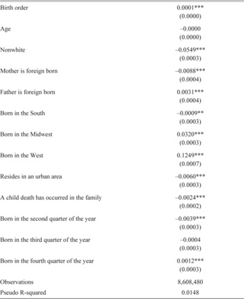
We run a probit regression to study the extent to which observables in 1900 relate to the likelihood of being matched to a record in 1940. Specifically, we study the effects of birth order, age (in 1900), whether the individual is white or not, whether the individual's mother was foreign born, whether the individual's father was foreign born, birth region (South, Midwest, West, and Northeast), an indicator for whether the individual resided in an urban area in 1900, quarter of birth, and an indicator for whether there have been any child deaths in the family. The indicator for child deaths is the closest measure of socioeconomic status that we are able to obtain. The average marginal effects are reported in Appendix Table 1. The only meaningful effects come from non-white and region of birth. Non-whites were 5 percentage points less likely to be matched to a record in 1940. Similarly, relative to those born in the South or the Northeast, those born in the West were 12.5 percentage points more likely to be found in 1940, and those born in the Midwest were 3 percentage points more likely to be found.
Annual City-Level Typhoid Data
Now that we have linked individuals between the two censuses, we now search for annual city-level typhoid data. We obtain typhoid fatality rates in the late nineteenth and early twentieth centuries for 75 cities. This data was transcribed from Whipple (Reference Whipple1908) as well as various issues of the U.S. mortality statistics. Figure 2 maps the cities used in our analysis. These cities tend to fall within the top 100 in terms of population. In 1900, they had an average population of 225,364 and a median population of 94,969. The cities are predominantly located in the Northeast and the Midwest but include all regions of the continental United States.

Figure 2 CITIES WITH TYPHOID DATA AND RIVERS
As a measure of early-life exposure to contaminated water, we average typhoid rates during the year of birth, the year before birth, and the year after birth. This has two advantages. First, because typhoid rates are volatile, the moving average provides a better proxy for average water quality. Second, the three-year moving average roughly corresponds with the prenatal, neonatal, and postnatal periods, which captures exposure during early life. Figure 3 plots the distribution of average typhoid rates during early life. The distribution is skewed right with a mean of 41.7 deaths per 100,000. The domain ranges from 10.4 deaths per 100,000 to 218 deaths per 100,000.

Figure 3 DISTRIBUTION OF TYPHOID RATES DURING EARLY LIFE
We merge these typhoid fatality data to linked micro data. This dataset links individuals observed in the 1940 and 1900 Censuses that were born between 1889 and 1899. We restrict our analysis to males who, at the time of the 1900 Census, were living in a city for which we have typhoid data. Because we treat the city of residence in 1900 as the birth city, we drop any individual that was born in a state other than their state of residence in 1900. We believe this assumption is reasonable given that the sample would be at most 11 years old in 1900.
Summary statistics are reported in Table 3. Age, education, income, homeownership status, and whether the individual moved from their birth city are taken from the 1940 Census. These outcome variables are measured during peak earning years (ages 40–51). The percent of blacks is small because our sample includes cohorts born in cities before the Great Migration. The average individual in our sample spent their early life in a city with an average typhoid rate of 42 deaths per 100,000.
Table 3 SUMMARY STATISTICS

Source:
Age, education, income, homeowner status, and whether the individual moved from their birth city are taken from the 1940 Census. Birth order was reported in the 1900 Census. Although the maximum of 91 is likely a typographical error, the 99th percentile of birth order, which is 10, is plausible. Typhoid data come from Whipple (Reference Whipple1908) and various issues of U.S. Mortality Statistics. Typhoid rate during early life is the average typhoid rate in the birth city from one year before birth, the year of birth, and one year after birth.
RESULTS
Ordinary Least Square (OLS) Results
In Table 4 we estimate the relationship between early-life typhoid and adult outcomes using the following equation:

where the outcome for individual i born in city j during year k is either years of schooling, ln(income), homeownership status, or mover/stayer status in 1940. Typhoid is the average typhoid rate during early life for individuals born in city j during birth year k, where early life is defined as the year before birth until the year after birth. We cluster standard errors at the birth-city level. Each regression includes fixed effects for each birth city, birth year, and birth order. Because outcomes are taken from the 1940 Census, controlling for birth year automatically controls for age. We find that typhoid during early life decreases educational attainment and adult income, but we find no effect on homeownership status or geographic mobility (mover/stayer status). These results indicate that if typhoid were eliminated, years of schooling would have increased by nearly one month and income would have increased by one percent.
Table 4 THE RELATIONSHIP BETWEEN TYPHOID AND ADULT OUTCOMES

* = Significant at the 5 percent level.
** = Significant at the 1 percent level.
*** = Significant at the 0.05 percent level.
†The average effect from eliminating typhoid is calculated by multiplying the coefficient for average typhoid rate during early life by –41.72, where 41.72 (deaths per 100,000) is the average typhoid death rate that individuals in our sample were exposed to during early life.
Notes:
Each regression controls for whether the individual is black or not. The regressions also include birth year, birth city, and birth order fixed effects. Robust standard errors (clustered at the city level) reported in parentheses.
Sources:
Typhoid data come from Whipple (Reference Whipple1908) and various issues of U.S. Mortality Statistics.
In our data, we find that typhoid epidemics during early life are negatively correlated with labor market outcomes, which suggests that the scarring effect dominates the selection effect. Because typhoid increased infant mortality (Cutler and Miller Reference Cutler and Miller2005), our sample likely suffers from survivorship bias. This would imply that our estimates are underestimates of the scarring effect. To better understand the extent to which selective mortality attenuates our results, we remove all cohorts whose average early-life typhoid exposure was greater than 99 deaths per 100,000 persons (the 95th percentile). Truncating the sample at the 95th percentile decreases the chance that our estimates of the scarring effect are confounded by survivorship bias. OLS results with this sample restriction are presented in Table 5. Consistent with attenuation, the effect of typhoid exposure is slightly larger when extreme epidemics are omitted. Specifically, we find that eliminating typhoid fever would have increased educational attainment by one and a half months and increased earnings by about 2.5 percent. Truncating the sample at the 75th, 90th, or 95th percentile produces qualitatively identical results.Footnote 7 This suggests that selective mortality is only a problem during extreme epidemics, which is also consistent with typhoid fever's low case fatality rate.
Table 5 OLS RESULTS OMITTING COHORTS WHOSE EARLY-LIFE TYPHOID RATE WAS GREATER THAN 99 DEATHS PER 100,000

* = Significant at the 5 percent level.
** = Significant at the 1 percent level.
*** = Significant at the 0.05 percent level.
†The average effect from eliminating typhoid is calculated by multiplying the coefficient for average typhoid rate during early life by –37.46, where 37.46 (deaths per 100,000) is the average typhoid death rate that individuals in our sample were exposed to during early life (after truncating at the 95th percentile).
Notes:
Each regression controls for whether the individual is black or not. The regressions also include birth year, birth city, and birth order fixed effects. Robust standard errors (clustered at the city level) reported in parentheses.
Sources:
Typhoid data come from Whipple (Reference Whipple1908) and various issues of U.S. Mortality Statistics.
OLS Robustness Checks
To illustrate that these results are driven by early-life exposure and not exposure during other ages, we estimate a variant of equation (2) that includes typhoid rates during the following years: seven to five years before birth; four to two years before birth; two to four years after birth; five to seven years after birth, as well as our measure of early-life exposure (one year before birth to one year after birth). Figure 4 plots the 95 percent confidence interval for these estimates. Consistent with Table 4, Figure 4 illustrates that early-life typhoid rates are associated with a decline in education and income in adulthood. No other periods are significant. Furthermore, the estimated relationship between early-life typhoid exposure and adult outcomes is similar to the estimates presented in Table 4. Although not presented in Figure 4, when the outcome is education, the coefficient on typhoid during early life is statistically different from any of the other lifecycle periods (at either the 1 or 5 percent level). The estimates for income, however, are less precisely estimated and so the coefficient on early-life exposure is only statistically different from one of the other lifecycle periods.

Figure 4 THE RELATIONSHIP BETWEEN AVERAGE TYPHOID RATES AT VARIOUS STAGES AND ADULT OUTCOMES
As an additional robustness check, we add state-of-birth-by-year-of-birth fixed effects to equation (2). These fixed effects control for any shocks that affected a single cohort at the state level. These shocks could include, compulsory schooling legislation, agricultural shocks and other state-level economic conditions, and exposure to extreme weather conditions. Similar to Table 4, the estimates in the first panel of Table 6 indicate that eliminating typhoid fever would have increased educational attainment by 0.09 years (significant at the 1 percent level) and increased earnings by 1.6 percent (significant at the 5 percent level). We find no evidence that exposure to typhoid during early life affected homeownership, but those that were exposed were less likely to move. Although these results are similar to Table 4, this is not our preferred specification because including state-by-year fixed effects absorbs all of the variation for states that only have one city in the sample.Footnote 8 This removes 19 cities from our sample including New Orleans, Baltimore, and Washington DC.
Table 6 ROBUSTNESS OF OLS RESULTS

* = Significant at the 5 percent level.
** = Significant at the 1 percent level.
*** = Significant at the 0.05 percent level.
†The average effect from eliminating typhoid is calculated by multiplying the coefficient for average typhoid rate during early life by –41.72, where 41.72 (deaths per 100,000) is the average typhoid death rate that individuals in our sample were exposed to during early life.
Notes:
Each regression controls for whether the individual is black or not. The regressions also include birth year, birth city, and birth order fixed effects. Robust standard errors (clustered at the city level) reported in parentheses.
Sources:
Typhoid data come from Whipple (Reference Whipple1908) and various issues of U.S. Mortality Statistics.
Our final robustness check concerns our birth-city assumption. We assume that all children under the age of 11 in 1900 resided in their city of birth so long as they were born in the same state. This is likely to attenuate the results because children born in the countryside, for instance, but migrated to the city before 1900 will be included in our analysis despite being exposed to a different disease environment. Approximately 6.8 percent of individuals under the age of 11 (that also resided in a city for which we have typhoid data) were born out of state. Older cohorts are less likely to reside in their city of birth than younger cohorts. To mitigate this problem we replicate Table 4 dropping all individuals born before 1895. These results are presented in the second panel of Table 6. The results are similar but slightly larger in magnitude, which is consistent with the attenuation argument discussed previously. Specifically, we find that eliminating typhoid fever would have increased education by about two months and increased earnings by about 2 percent. We also find that those exposed to typhoid were less mobile.
Semi-Parametric Results
A concern with the analysis previously is that it imposes a linear relationship on the data when the data might in fact be related in non-linear ways. To address this concern, we estimate the relationship between typhoid and adult outcomes semi-parametrically. Specifically, we estimate the following equation:

This equation is similar to equation (2) except that it does not impose a linear relationship between early-life typhoid exposure and adult outcomes. We non-parametrically estimate the relationship between early-life typhoid exposure and adult outcomes using linear partial regression. However, this requires a strict ordering of early-life typhoid rates. We achieve this by collapsing the data at the city-year level.Footnote 9 Since we collapse at the city-year level, blackjk becomes the percent of the cohort born in city j during year k that is black, and birth orderjk becomes the average birth order for individuals born in city j during year k.
Figure 5 presents the non-parametric estimates of f(Typhoid). Early-life exposure to typhoid decreases adult earnings and educational attainment above the 10th percentile of the early-life typhoid distribution. Moreover the relationship is approximately linear. Moving from the top of the typhoid distribution to elimination would have increased educational attainment by one-third of a year and increased earnings by about 4 percent. There does, however, appear to be a positive relationship between zero and 20 deaths per 100,000, but this constitutes less than 10 percent of our sample.Footnote 10 Overall then, it appears that the linear model adopted in the previous section is appropriate.

Figure 5 SEMI-PARAMETRIC ESTIMATES OF THE RELATIONSHIP BETWEEN TYPHOID AND ADULT OUTCOMES
Two-Stage Least Squares Results
One might be concerned that typhoid during early life is correlated with variables we cannot observe or otherwise directly control for. In particular, two competing hypotheses seem plausible. First, investment in water filtration might be correlated with unobservable investments that also increase human capital. In this case, our OLS estimates would overstate the benefits of water filtration and purification on later life economic outcomes. Second, and alternatively, there was a heavy mortality penalty for living in large, fast growing cities, and this penalty grew larger as city size grew (Cain and Hong Reference Cain and Hong2009; Haines Reference Haines2001). This suggests that typhoid rates might have been the highest in years of unusually rapid economic growth, and to the extent that we do not fully control for such growth, high typhoid rates might conflate the beneficial health effects of being exposed to economic growth (and high income) early in life with the deleterious effects of impure water. If so, one would want to look at a measure of water quality that captured the effects of only water quality and not economic activity. In the absence of such a measure, our OLS estimates would understate the benefits of water filtration.
To address these concerns, we implement an instrumental variables (IV) strategy. This strategy builds on the following logic: because typhoid is a waterborne disease, cities that dump their sewage into a river will increase future typhoid rates for cities downstream. Additionally, the typhoid rates in cities upstream should be exogenous to human capital investments in the receiving city. Because typhoid fever was also sometimes spread through milk, one might be concerned about overlapping dairy markets as a threat to our exclusion restriction. During our sample period (1890–1900), however, milk-borne epidemics were comparatively rare. Furthermore, dairy markets were highly localized for all but the biggest cities during this time, typically concentrated in a 60-mile radius around the city (Rosenau Reference Rosenau1912, pp. 16–20). Because the mean distance between the upstream and downstream cities in our sample is 174 miles, it seems unlikely that upstream milk markets would have influenced downstream typhoid rates. The localization of milk markets was driven by the fact that milk was not transported in refrigerated rail cars during the 1890s and early 1900s (U.S. Public Health and Marine Hospital Service 1912).
Eighteen of the 75 cities used in the previous analysis lie downstream from another city for which we have typhoid data. We confirm flow direction for each river using data from the United States Geological Survey.Footnote 11 Cities that are upstream (the feeder cities) dump their sewage into the river. This increases the typhoid rates in cities downstream (the receiving city). Thus, we use typhoid rates in the feeder city as an instrument for typhoid rates in the receiving city. Whether we should use contemporaneous typhoid rates or the rates lagged by one year depends on the distance between the two cities and the flow rate of the river. We find similar results regardless of whether we use the contemporaneous or lagged typhoid rate, but lagged typhoid rates produce a stronger first stage.
Because only a subset of our initial sample lies downstream from another city for which we have typhoid data, it is perhaps useful to show that our main results hold for this subset of cities. Accordingly, we replicate our main analysis (restricting to the set of downstream cities) in Table 7.Footnote 12 The results are slightly larger but qualitatively similar to the main results presented in Table 4. Specifically, we find that eliminating typhoid fever would have increased educational attainment by 1.4 months instead of 1.1 and would have increased adult earnings by about 1.7 percent instead of 1.3.
Table 7 THE RELATIONSHIP BETWEEN TYPHOID AND ADULT OUTCOMES (IV SAMPLE ONLY)

* = Significant at the 5 percent level.
** = Significant at the 1 percent level.
*** = Significant at the 0.05 percent level.
†The average effect from eliminating typhoid is calculated by multiplying the coefficient for average typhoid rate during early life by –41.72, where 41.72 (deaths per 100,000) is the average typhoid death rate that individuals in our sample were exposed to during early life.
Notes:
Each regression controls for whether the individual is black or not. The regressions also include birth year, birth city, and birth order fixed effects. Robust standard errors (clustered at the city level) reported in parentheses.
Sources:
Typhoid data come from Whipple (Reference Whipple1908) and various issues of U.S. Mortality Statistics.
Table 8 presents our results using lagged typhoid rates in the feeder city as an instrument for typhoid rates in the receiving city. Lagged typhoid rates in the feeder city are a strong predictor of typhoid rates in the receiving city; an additional 100 deaths per 100,000 in the feeder city increases the typhoid death rate in the receiving city by eight in the following year. The F-statistics associated with this estimate range from 517.81 to 671.12 and therefore suggest that lagged typhoid rates from the feeder city are a strong instrument. In the second stage we find that typhoid rates during early life decrease educational attainment and earnings, although only the first estimate is statistically significant at the 5 percent level.Footnote 13 The estimate on earnings, while imprecisely estimated, has the same sign and much larger coefficient in absolute value than the OLS results. These results indicate that eliminating typhoid would have increased schooling by nine months, and would have increased income by 9.8 percent. Table 8 also indicates that high typhoid rates during early life reduced mobility, that is, the likelihood that the individual would reside in their birth city as an adult. The results here are considerably larger in magnitude than those obtained with OLS. Using a Durbin-Wu-Hausmann test, we can reject the null hypothesis that the two coefficients are the same at the 10 percent level. This suggests that the difference in magnitudes stems from the fact we not able to fully control for the effects of positive economic growth using OLS.
Table 8 2SLS ESTIMATES OF EARLY-LIFE TYPHOID ON ADULT OUTCOMES

* = Significant at the 5 percent level.
** = Significant at the 1 percent level.
*** = Significant at the 0.05 percent level.
†The average effect from eliminating typhoid is calculated by multiplying the coefficient for average typhoid rate during early life by –41.72, where 41.72 (deaths per 100,000) is the average typhoid death rate that individuals in our sample were exposed to during early life.
Notes:
Each regression controls for whether the individual is black or not. The regressions also include birth year, birth city, and birth order fixed effects. Robust standard errors (clustered at the city level) reported in parentheses.
Sources:
Typhoid data come from Whipple (Reference Whipple1908) and various issues of U.S. Mortality Statistics.
COST-BENEFIT ANALYSIS
The previous section illustrates that eliminating typhoid fever would have increased educational attainment by one to nine months and increased income by one to nine percent. These estimates raise the question of whether the net present value of the increase in wages was enough to offset the costs associated with eliminating typhoid fever. Cutler and Miller (Reference Cutler and Miller2005) have analyzed the benefits of adopting water purification technologies using the value of a statistical life and find that the benefits outweigh the costs by a ratio of 23 to 1. In our analysis, we ignore the gains from additional life years and instead focus on whether the discounted increase in earnings would have been sufficient to cover the costs of eliminating typhoid fever.
To analyze the benefits from typhoid elimination, we need the following information: the probability that an individual survives to a given age with and without the intervention, average income by age with and without the intervention, and the number of individuals in a cohort who would benefit from the water infrastructure. To analyze the costs, we need to know the total costs of municipal water systems and how frequently these systems need to be replaced. Lastly, to compare the net present values, we need real interest rates.
Eliminating typhoid fever has two effects on wages. First, it increases the average wage. Second, it increases the probability that an individual will survive until that age. The survival probability, Sa , is the probability that an individual survives to age a. We use the survival probabilities for males born in 1900 from the Social Security life tables. Cutler and Miller (2005) find that mortality fell by 13 percent after the introduction of clean water technologies. Accordingly, we adjust the 1900 survival probabilities to reflect this change. We use the 1940 Census to obtain the wage profile for males. Specifically, we obtain average earnings by age using a local polynomial smooth for all males. For the counterfactual wage distribution, we scale these averages by 1 to 9 percent, which corresponds to the OLS and IV estimates, respectively.
We assume that the average cohort of males born in a city is 20,000, which is approximately the number of males born in Chicago in 1900.Footnote 14 Finally, to obtain the costs we use the numbers reported in Cutler and Miller (Reference Cutler and Miller2005), which assumes that the average cost of the waterworks for a large city was 22.8 million dollars in 1940 and that the waterworks must be replaced every ten years. These assumptions underestimate the gains from eliminating typhoid fever. First, we assume that female earnings were unaffected by typhoid. Second, we assume that the only benefit from reduced mortality was increasing the probability of receiving future earnings. Third, we assume that the entire waterworks must be replaced every ten years, when in reality many parts are likely to function for longer. Furthermore, we assume that the construction of the waterworks was necessary to eliminate typhoid fever, but one could argue that the marginal cost of chlorinating or filtering water was sufficient to eliminate typhoid fever.
We calculate the benefits to eliminating typhoid fever using equation (4), where S a′ is the counterfactual survival probability and Wa ′ is the counterfactual wage. The waterworks lasts T years, N is the cohort size, and r is the real interest rate.

This equation allows us to compute a break-even point for eliminating typhoid fever. The increase in earnings alone was sufficient to offset the cost of eliminating typhoid fever for any real interest rate under 7 percent (using our OLS estimates) or 10 percent (using our IV estimates). Using an interest rate of 3.12 percent, the average interest rate for high-grade municipal bonds in 1900 (Homer and Sylla Reference Homer and Sylla2005, p. 341), we find that the increase in wages exceeded the costs of eliminating typhoid by nearly 80 million dollars (under OLS) or 230 million dollars (under IV).
CONCLUSION
Between 1900 and 1940 mortality in the United States fell by nearly 40 percent. Approximately half of this decline was the result of investment in water purification technologies and the elimination of waterborne diseases such as typhoid fever. There have been a number of previous studies estimating the social rate of return to water purification measures, but all of these studies focus on the gains associated with reductions in mortality (e.g., Cutler Miller Reference Cutler and Miller2005; Ferrie and Troesken Reference Ferrie and Troesken2008). Yet because typhoid was such a virulent disease and had such a low case fatality rate, there is good reason to believe that its effects on morbidity and long-term human capital formation were substantial. Accordingly, in this article, we explore how eliminating early-life exposure to typhoid fever affected economic outcomes in later life. Our laboratory consists of urban residents in large American cities during the late-nineteenth and early twentieth century.
In our analysis, we explore how early-life exposure to typhoid fever (our primary indicatory of water quality) influenced later life outcomes in terms of income, educational attainment, home ownership, and geographic mobility. Using parametric, semi-parametric, and IV approaches, our results indicate that eliminating typhoid fever, which cities achieved by adopting clean water technologies, would have increased educational attainment by one to nine months and earnings by between one and nine percent. A simple cost-benefit analysis reveals that the increase in earnings from eliminating typhoid fever was more than sufficient to offset the costs of elimination. When one considers that our calculations ignore the changes in mortality captured by Cutler and Miller (Reference Cutler and Miller2005) and other researchers, the evidence that investments in water purification have very high rates of social return seems unassailable. These results have important policy implications for developing countries that have yet to adopt water purification technologies.
Appendix
Appendix Table 1 PROBIT ESTIMATES OF 1900 OBSERVABLES ON SUCCESSFUL LINK TO 1940 CENSUS