


1. Introduction
Rapid mass movements, such as snow avalanches, landslides and debris flows, are common in mountain regions. One shared feature of these flows is their granular nature. Commonly, these flows may also be destructive, posing severe hazards to human lives and infrastructures. A usual way to reduce their catastrophic potential is to consider building structures aimed at slowing down the flow and diverting it (Pudasaini et al. Reference Pudasaini, Hutter, Hsiau, Tai, Wang and Katzenbach2007; Johannesson et al. Reference Johannesson, Gauer, Issler and Lied2009; Sovilla et al. Reference Sovilla, Sonatore, Bühler and Margreth2012; Iverson, George & Logan Reference Iverson, George and Logan2016; Albaba, Lambert & Faug Reference Albaba, Lambert and Faug2018). When the granular flow hits such structures, the velocity of the granular mass decreases, and the flow thickens and becomes denser. This transition from a fast, thin flow into a slow thicker one is known as a jump (Gray, Tai & Noelle Reference Gray, Tai and Noelle2003). In this process, the final, steady-state flow height is critical for designing protective structures.
Granular jumps tend to form when flowing granular materials meet sharp changes in the slope along their path, such as along natural topographies above which avalanches and landslides propagate. A most prominent example for sharp changes causing such jumps occurs when the slopes transition from initial steep sections into run-out zones with lower inclinations (Tai & Lin Reference Tai and Lin2008) or bump-like obstacles (Viroulet et al. Reference Viroulet, Baker, Edwards, Johnson, Gjaltema, Clavel and Gray2017). Granular jumps also develop in various industrial settings involving the transportation of particles in silos, pipes or chutes (Samadani, Mahadevan & Kudrolli Reference Samadani, Mahadevan and Kudrolli2002; Jaworski & Dyakowski Reference Jaworski and Dyakowski2007; Xiao et al. Reference Xiao, Hruska, Ottino, Lueptow and Umbanhowar2018). Understanding granular jumps is crucial for mitigating the associated risks and optimizing their industrial applications. An initial approach for their understanding considers an incompressible flow as proposed by Chanson (Reference Chanson2009). While this approach may be suitable for nearly subcritical flows, compressibility becomes relevant with increasing velocity, where incoming flows become considerably diluted, bringing a substantial increase in density through the jump. Later studies on granular jumps have demonstrated that the length of compressible jumps is relevant due to energy dissipation from both short-lived collisions and long-enduring frictional contacts between the particles and the base (Méjean, Faug & Einav Reference Méjean, Faug and Einav2017).
Considering the relevance of friction in granular jumps, this study presents a detailed numerical analysis of the jump length over a wide range of incoming flow conditions, focusing on the effect of slope bottom friction and interparticle friction. The numerical set-up presented here considers two-dimensional (2-D) and three-dimensional (3-D) flows down smooth inclines, which impact a wall located at the end of a chute, thus forming upon impact a jump that travels upstream. During this process, the opening height of an outgoing gate located at the end of the chute is adjusted, aiming to equalize the incoming and outgoing flow fluxes. By doing so, the jump is tuned to remain stationary at a fixed position along the chute. Under such steady-state conditions, the jump is defined as a standing jump, allowing its properties to be averaged in time for effective analysis and interpretation of the physical parameters determining its length.
In order to deliver the last point, the paper is organized as follows: in § 2, we describe the numerical set-up and procedures. In § 3, we present the obtained results, which focus on the main physics of the incoming flow. Next, we examine the jump length measurements. In § 4, we introduce a scaling law for the jump length and discuss its implications. Finally, in § 5, we summarize our results and draw the main conclusions.
2. Methods
2.1. Numerical set-up
Standing granular jumps are simulated with the discrete element method (DEM) using the open-source software YADE (Smilauer Reference Smilauer2021). These simulations involve spherical grains of diameter  $d$ whose interactions are being controlled by a viscoelastic contact model for the normal forces and an elastic force limited by a Coulomb friction threshold for tangential forces, as proposed by Pournin, Liebling & Mocellin (Reference Pournin, Liebling and Mocellin2001). The normal viscoelastic force is controlled by a linear spring proportional to the normal overlap between grains with stiffness $k_n=Ed/2$ and a dashpot defined by a damping coefficient. The constant $E$ is set to $1\times 10^{6}$ and $1\times 10^{7}$ Pa for 2-D and 3-D simulations, respectively, with a typical range of $10^{-3}$– $10^{-4}$ for the maximum values of the ratio of the overlap to the grain diameter. Similarly, the damping coefficient is determined by the grains’ restitution coefficient $e$, which was set as $0.5$. Poisson's ratio $\nu$ was taken equal to $0.3$, leading to a tangential stiffness $k_t=\nu k_n$. The material density of the grains $\rho _p$ was defined at $2500$ kg m $^{-3}$ to mimic glass beads typically used in experimental works. Time step $dt$ was set as $3\times 10^{-4}$ s for the 2-D simulations and decreased to $3\times 10^{-5}$ s for the 3-D simulations, following the suggested values by O'Sullivan & Bray (Reference O'Sullivan and Bray2004). The grains are spherical and their mean diameter $d$ was set as $4$ cm with a size distribution of ${\pm }15\,\%d$ to avoid crystallization effects. A few additional simulations were performed using mean diameters of $2$ and $6$ cm to explore the possible influence of the grain diameter on the jump. The friction along the bottom of the chute was set based on the coefficient $\mu _b$ ranging from $0.0315$ to $0.72$. The grains’ internal friction coefficient $\mu$ was varied between $0.25$ and $0.72$. The combination of these friction coefficients was selected so that their ratio would follow $\mu /\mu _b\leq 1$. Finally, the flume inclination angle $\zeta$ varied from $8.5$ to $48$ degrees. The simulation set-up follows a similar one used by Méjean et al. (Reference Méjean, Guillard, Faug and Einav2020), as depicted in figure 1. Two-dimensional simulations were performed using spheres (instead of disks) aligned to the $y$-axis with their respective rotations and displacement degrees of freedom restricted around this axis. In the 3-D case, periodic boundaries (also known to set so-called ‘unconfined flows’) were implemented normal to the flow direction ( $y$-axis in figure 1) with a distance (width) between them of $10d$. The gate opening height $H$, which controls the mass discharge, was set at $H/d=10$, $15$ and $20$. The measurements of both the incoming and outgoing flow fluxes ( $Q_1$ and $Q_2$) were performed every 30 time steps (see details in § 2.2). Here $Q_1$ was measured by counting the grains leaving the reservoir, while an equivalent number of grains were added on top of the reservoir in order to ensure it remained full. Similarly, $Q_2$ was measured by counting the grains that passed through the outgoing gate during the same time period, while these counted grains were removed from the simulation.

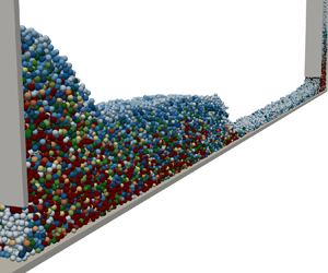
Figure 1. (a) Sketch of a typical simulated granular jump. The circular-shaped inset shows the velocity profile  $u(z)$ close to the smooth bottom with slip velocity $u_s$, as systematically observed in figure 2. (b) Snapshots from 2-D (top) and 3-D (bottom) DEM simulations. Examples with $\zeta =24\deg, H/d=10, \mu _b=0.24, \mu =0.54, d=4$ cm. In all panels, g refers to gravity acceleration $g = 9.81\ {\rm m}\ {\rm s}^{-2}$.
2.2. Numerical procedure
Standing jumps are generated by releasing grains from the tank and controlling the outgoing flow at the bottom of the chute. Initially, the reservoir is filled with grains to a height of at least  $3H$. In the second, phase the reservoir gate gets opened while the outgoing gate is being closed ( $Q_1\neq 0, Q_2=0$). During this phase, the bulk of the grains starts flowing down the chute and later hits the initially closed outgoing gate. In this process, a travelling wave known as a granular bore (Gray & Hutter Reference Gray and Hutter1997; Albaba et al. Reference Albaba, Lambert and Faug2018) forms. As the bore gets approximately to the centre of the chute, the outgoing gate is opened to let the grains release from the bottom of the chute. In the next phase, the height of the outgoing gate is adjusted up and down until a steady state is being reached so that the bore's position remains stationary, thus forming what is known as a standing granular jump (see examples depicted in figure 1). We define the steady state to denote events where the average value of both $Q_2$ and $Q_1$ over the last five measurements falls within a 15 % tolerance of each other. Once this steady state is achieved, we record the coordinates and velocities of all grains, at least 10 times, with a gap of 0.3 seconds between each recording. This rate of recordings was empirically found to provide a sufficiently smooth signal to properly study and define the steady-state jump. A greater number of recordings was used on certain simulations, but little difference was observed. In order to achieve a smooth signal, we implemented the coarse-graining procedure from Hoover & Hoover (Reference Hoover and Hoover2006) to measure the fields of volume fractions and mean velocities. This coarse-graining was performed using spatial windowing based on Lucy polynomials on a uniformly distributed grid with a spacing of $0.25d$ between nodes. Each node's calculation considered the spheres within a radius of $2.5d$ from that node, based on the previous 2-D numerical study and sensitivity analysis in Méjean et al. (Reference Méjean, Guillard, Faug and Einav2020). Given that in the 3-D simulations the flows are found to be homogeneous across the flume width due to the periodic boundaries, in those simulations the coarse-graining was performed only at the centre of the chute along the $x$-axis. The free-surface height along the chute $h(x)$ was defined from the coarse-grained solid fraction $\phi$ field using a limit value $\phi _{lim}$ used to indicate the transition from liquid to the gaseous regime. The value of $\phi _{lim}$ was set at $0.15$ for 2-D simulations, as defined by Méjean et al. (Reference Méjean, Guillard, Faug and Einav2020). For 3-D simulations, $\phi _{lim}$ was adjusted to $0.11$ in proportion to the difference between the random close packing values measured from the simulations: $0.83$ and $0.64$ for the 2-D and 3-D cases, respectively. After the free surface is defined, data are depth-averaged to obtain velocity magnitudes and volume fractions along the $x$ direction, denoted as $\bar {u}(x)$ and $\bar {\phi }(x)$, respectively. These depth-averaged signals are smoothed using a 2nd-order Butterworth filter (Selesnick & Burrus Reference Selesnick and Burrus1998) with a critical lowpass frequency of $0.06$ m $^{-1}$. The filter is adjusted to provide the smoothest signal while maintaining the positions of any peaks in the signal. The jump length $L$ is measured based on $\bar {u}(x)$ and its derivative with respect to the $x$-axis ( ${\rm d}\bar {u}(x)/{{\rm d}\kern 0.06em x}$). The jump produces an abrupt drop in the velocity, as seen in figure 1(b). This drop in velocity is then used to determine the jump limits. The jump starts at the position where the flow begins to decelerate across the chute after leaving the tank ( ${\rm d}\bar {u}(x)/{{\rm d}\kern 0.06em x}=0$). Considering this identified position, we measure the depth-averaged volume fraction and velocity for the jump ( $\bar {\phi }$ and $\bar {u}$ respectively). The depth-averaged jump density $\bar {\rho }$ at the start of the jump is defined as $\bar {\rho }= \bar {\phi } \rho _{p}$. The end of the jump is identified by analysing the variation of ${\rm d}\bar {u}(x)/{{\rm d}\kern 0.06em x}$ through the Matlab function findchangepts(), which is used to detect the end of the abrupt change produced by the jump. Flow variables at the end of the jump are denoted with the subscript $_*$ (see figure 1). A spreadsheet of all these results is available from the supplementary data available at https://doi.org/10.1017/jfm.2023.757.
2.3. Froude numbers
In the following, we present results in terms of dimensionless groups. In former studies about granular jumps, by analogy to hydraulic jumps, the Froude number is commonly defined as
 \begin{equation} Fr(x) = \bar{u}(x) / \sqrt{gh (x)\cos \zeta}. \end{equation}
However, for the present work, the Froude number will be defined as
 \begin{equation} \mathcal{F}(x) = \bar{u}(x) / \sqrt{gh (x) \bar{\phi} (x) \cos \zeta}. \end{equation}
 In the above definition, the depth-averaged volume fraction is considered as we found that it improves the correlation between the measured jump length and the corresponding Froude number in § 3.2 (see figure 3). This slight modification of the Froude number is consistent with previous studies that rely on the depth-integrated volume fraction  $\smallint _0^\infty \phi (z)\,{\rm d} z= h\bar {\phi }$, called the mass hold-up (Louge & Keast Reference Louge and Keast2001; Zhu, Delannay & Valance Reference Zhu, Delannay and Valance2020), for granular flows down a smooth bottom. Note that in the present study, the integral is bounded by the flow height, defined from $\phi _{lim}$. In addition to $\mathcal {F}$ above, it is found useful to define another Froude number, this time corresponding to the base of the flow:
 \begin{equation} \mathcal{F}_s(x)=u_s(x)/\sqrt{gd\cos\zeta}, \end{equation}
where  $u_s$ refers to the slip velocity on the base, defined as the averaged velocity over one grain diameter distance from the bottom, as sketched in the circular-shaped inset of figure 1. Here $\mathcal {F}_s$ is proposed in addition to $\mathcal {F}$ so that we could account for the sliding at the smooth bottom and its interplay with the bulk deformation across the entire flow thickness.

Figure 2. Influence of  $\mu _b$ on velocity profiles at jump start for 2-D (a) and 3-D (b) simulations. Dashed lines in (a,b) refer to the Bagnold profile best fit. (c) Influence of $\mu _b$ on $\bar {u}/\sqrt {gd}$ and $h/d$. Examples for $\zeta = 24\,\deg$, $d=4$ cm, $\mu =0.54$ and $H/d=15$.

Figure 3. (a) Normalized jump length  $L/d$ vs Froude number $\mathcal {F}$ for different $\mu _b/\mu$. In inset: an example for all 3-D periodic jumps for different opening heights of the tank ( $\mu _b=0.25$, $\mu =0.54$). Panels (b,c) show the streamlines for two extreme jumps (data shown in inset of (a)): steep jump with recirculation (b) and laminar jump (c).
3. Results
3.1. Incoming flow
In the simulations, the incoming flow does not appear to be affected by the jump. This can be understood due to the supercritical nature ( $\mathcal {F}>1$) of the flow, which moves faster than the downstream influence of the jump can propagate upstream. Additionally, as described in Méjean et al. (Reference Méjean, Guillard, Faug and Einav2020), the simulations show that the detectable rise in the free surface produced by the jump only occurs downstream, after the jump start. Velocity profiles at the position across the flume where the jump starts are strongly influenced by $\mu _b$ when all the other parameters remain unchanged, as seen in figure 2(a,b). Furthermore, a theoretical Bagnold profile with slip at the base is shown to fit well the incoming flow profiles, especially in the 2-D simulations where the fit remains good even for high $\mu _b$ (see figure 2a).
All velocity profiles show some level of sliding at the base of the flow. These profiles show a transition from purely plug-like shallow flows ( $u_s/\bar {u}=1$) for low $\mu _b$ to thicker sheared flows, yet still with a significant sliding at the base for high $\mu _b$. These normalized plots highlight the transition between plug-like flows that are essentially controlled by the slip velocity at the bottom and flows that still slip significantly but with a well-established shear profile that develops across the bulk when increasing $\mu _b$. Moreover, as illustrated in figure 2(c), an increase in $\mu _b$ leads to a decrease in the incoming velocity of the flows while simultaneously increasing the flow height, a trend observed in both 2-D and 3-D simulations.
3.2. Jump length
Figure 3(a) shows the dependence of the normalized jump length  $L/d$ on the Froude's number $\mathcal {F}$ at jump start. Upon the normalization of $L$ by $d$ the results generally collapse independently to grain diameter $d$. On the contrary, the results are more scattered for different flow heights observed in the inset of figure 3(a). Varying $\mu _b$ and $\mu$ also contributes to the scatter of the data observed in figure 3(a). In spite of that scattering, this figure also displays two important asymptotic regimes in terms of jump length. The first asymptotic regime takes place at high $\mathcal {F}$ values, where the jump length tends to a constant value, which is approximately $50d$ in our numerical simulations. In this regime, steep colliding jumps occur (see figure 3b), as named by Méjean et al. (Reference Méjean, Guillard, Faug and Einav2020). The second asymptotic regime appears when $\mathcal {F}$ approaches the critical flow state ( $\mathcal {F}\approx 1$), where $L/d$ diverges, meaning a regime with very elongated jumps. These jumps possess a ‘laminar’ shape (see figure 3c) based on descriptions and terminology in Méjean et al. (Reference Méjean, Guillard, Faug and Einav2020). This shape will ultimately elongate until no jump occurs. The transition between laminar and steep colliding jumps identified in previous experimental studies (Gray et al. Reference Gray, Tai and Noelle2003; Faug et al. Reference Faug, Childs, Wyburn and Einav2015) remains blurry, which possibly explains the observed scattering in $L/d$ on figure 3(a). This scattering will be resolved in the next section. Finally, it is worth noticing that 3-D jumps have a shorter length than 2-D jumps with similar $\mathcal {F}$ of the incoming flow. This point will be further discussed in the next section.
4. Discussion
4.1. A scaling law for the jump length
The scattering on figure 3(a) is significantly reduced when normalizing  $L/d$ by the basal Froude number $\mathcal {F}_s$, as shown in figure 4. The obtained results show a strong collapse, and thus it could be concluded that it is crucial to account for the sliding at the smooth bottom. The results can be fitted through the function $L/(d \mathcal {F}_s)=\alpha /(\mathcal {F}-1)$ (thus ensuring that $L$ diverges when $\mathcal {F}$ reaches unity) which can be further expressed as
 \begin{equation} \frac{L}{d}= \alpha\frac{\mathcal{F}_s}{\mathcal{F}-1}=\alpha \sqrt{\frac{h\bar{\phi}}{d}}\frac{u_s}{\bar{u}}\frac{\mathcal{F}}{\mathcal{F}-1}, \end{equation}
where  $\alpha$ is a parameter that depends on the system dimension (see obtained values for 2-D and 3-D systems in the inset legend of figure 4). Scaling using $Fr$ was also considered but led to a poorer collapse of the data. The proposed fit above allows us to describe the jump length in a way that relies only on the depth-averaged flow properties ( $\bar {u}$ and $\bar {\phi }$), height $h$ and the sliding velocity $u_s$, regardless of the previously described scattering produced by both the bottom friction $\mu _b$ and the opening height $H$ of the tank, but accounting for the crucial interplay between the amount of sliding at the bottom and shearing across the granular bulk above. Regarding the regime described earlier in § 3.2, where $L$ diverges when the input condition approaches the critical state ( $\mathcal {F}\approx 1$) as seen in figure 3(a), the proposed scaling in (4.1) takes into account the decrease in $u_s$ as seen in figure 4, which helps to maintain the divergence of $L$. This behaviour is consistent because when the incoming flow approaches subcritical conditions, the sliding at the bottom may vanish while the jump extends over the whole length of the chute. When this occurs, it is less easy for the grains to cross the jump, and the already laminar jump becomes even more diffused. An (extreme) virtual situation occurs when the jump extends over the total length of the chute, which requires the incoming and the outgoing flow fluxes to be the same (subcritical condition reached everywhere). In the other asymptotic regime, the jumps become steeper as the $\mathcal {F}$ value increases, resulting in a higher $h_*/h$ ratio. Steeper jumps resemble those obtained in Pudasaini et al. (Reference Pudasaini, Hutter, Hsiau, Tai, Wang and Katzenbach2007) and Méjean et al. (Reference Méjean, Guillard, Faug and Einav2020). Recirculation starts to appear as a transition towards a fully steep colliding jump (refer to figure 3b), also consistent with the definition provided by Méjean et al. (Reference Méjean, Guillard, Faug and Einav2020). Although improved relative to figure 3 there are still some differences between the 2-D and the 3-D simulations in figure 4. Specifically, the 3-D jumps are shorter (lower $L/d\mathcal {F}_s$) than the 2-D jumps for the measured values of $\mathcal {F}$, suggesting that macroscopic friction is higher in 3-D than in 2-D for similar $\mathcal {F}$. In other systems (e.g. $h_{stop}$ curves for granular flows down rough inclines (GDRMidi 2004), run-out distance in granular column collapse (Utili, Zhao & Houlsby Reference Utili, Zhao and Houlsby2015)), macroscopic friction is also generally higher in 3-D than in 2-D. In this context, the jump length represents a proxy to the availability of the granular material to dissipate energy. Shorter jumps mean more dissipative granular bulks compared with longer jumps.

Figure 4. Scaling for the jump length using the depth-averaged Froude number  $\mathcal {F}$ based on mass hold-up and the basal Froude number $\mathcal {F}_s$. Here, $R^2$ is the coefficient of determination for the fits based on (4.1). Inset: same data in logarithmic scales.
4.2. Bottom slip velocity and improved scaling for jump length
Although the jump length can already be expressed through (4.1), the sliding velocity is not considered in the jump framework proposed by Méjean et al. (Reference Méjean, Faug and Einav2017). Moreover,  $u_s$ can be challenging to estimate when considering specific geophysical flows. A relationship between the sliding velocity and the depth-averaged velocity is thus proposed:
 \begin{equation} u_s=\beta\bar{u} \left(\frac{d}{h}\bar{\phi} \right)^{0.1}, \end{equation}
where  $\beta$ is a coefficient that depends on the dimension of the system (see figure 5). This relationship can be seen as a modification of the empirical law proposed by Zhu et al. (Reference Zhu, Delannay and Valance2020) for granular flows down smooth inclines yet with sidewalls: in particular, see (2) in Zhu et al. (Reference Zhu, Delannay and Valance2020) that yields $u_s\approx \bar {u}/(h\phi /d)^{1/4}$. The latter scaling is different from (4.2) as the exponents vary, particularly the exponent for $h$ which is negative. We do not have a clear explanation to this finding, except recalling that the present study considers unconfined flows while Zhu et al. (Reference Zhu, Delannay and Valance2020) were investigating confined flows with sidewalls. Nevertheless, this is an empirical way to describe the crucial interplay between apparent sliding at the smooth bottom and the granular bulk, while getting rid of the sliding velocity, which thus becomes a function of depth-averaged features ( $\bar {u}$, $h$ and $\bar {\phi }$) of the incoming flows. Note that the slip velocities measured in our simulations could be used in the future as a test bed for future advancement of the theory by Louge & Keast (Reference Louge and Keast2001). It is important to stress that the contribution of the slip velocity to depth-averaged velocity is largely dominant here for the case of a smooth incline, as depicted in figure 2 (Brodu, Richard & Delannay Reference Brodu, Richard and Delannay2013; Faug et al. Reference Faug, Childs, Wyburn and Einav2015; Zhu et al. Reference Zhu, Delannay and Valance2020). This is significantly different from the case of granular flows down a rough incline with no slip velocity or negligible $u_s$ (Louge Reference Louge2003; GDRMidi 2004).

Figure 5. (a) Scaling for sliding velocity  $u_s$ considering (4.2); (b) $u_s$ vs $\bar {u}$ with a bigger scatter of data at higher $\mu _b$, despite the practically apparent linear trend.
The jump length relative to the grain diameter can be predicted through the new scaling:
 \begin{equation} \frac{L}{d}= \gamma \bar{\phi}^{0.6}\left(\frac{h}{d} \right)^{0.4}\frac{\mathcal{F}}{\mathcal{F}-1}, \end{equation}
where  $\gamma =\alpha \beta$. The accuracy of the approach proposed in (4.3) is verified in figure 6.

Figure 6. Predicted jump length  $L_P$ against measured jump length $L_M$: (a) 2-D results, (b) 3-D results. Insets are the histogram of error, defined as $2(L_P-L_M)/(L_P+L_M)$.
4.3. Jump length–height ratio
The importance of predicting the jump length is its use in closing the augmented Bélanger equation by Méjean et al. (Reference Méjean, Faug and Einav2017). In that framework, the jump length appears in the form of the ratio  $L/h$. By using (4.3), the ratio $L/h$ is given by the following empirical law:
 \begin{equation} \frac{L}{h}= \gamma \left(\bar{\phi}\frac{d}{h}\right)^{0.6}\frac{\mathcal{F}}{\mathcal{F}-1}. \end{equation}
 Figure 7 shows the prediction of  $L/h$ using the above empirical scaling against the corresponding measured data for both the 2-D and 3-D cases. Regarding the 2-D case, some comments can be made: high values of $L/h$ are generally obtained for higher $\mu _b/\mu$, the highest measured $L/h$ can reach ${\approx }45$, and predictions are not good for $L/h>25$. For the 3-D system, the measured $L/h$ values span a narrower range ( $\approx$6–15), which is less than in the 2-D case. Moreover, the trend that increasing $\mu _b/\mu$ tends to generally decrease $L/h$ is also seen (see legend colour for $\mu _b/\mu$ in figure 7). The prediction of (4.4) is better and is generally very reasonable, though some data points spread away from the line of equality.

Figure 7. Predicted jump length ratio  $L_{P}/h$ vs measured $L_{M}/h$ for 2-D (a) and 3-D (b) cases. The dashed line shows the line of equality in both plots.
5. Summary and conclusions
This work presents the results of extensive 2-D and 3-D simulations of standing jumps along inclined planes developed using the DEM. During the simulations, multiple input parameters were systematically varied to obtain a wide range of granular jump patterns. The granular flows and jumps are found to be strongly influenced by the interplay between the sliding of the first layer of grains on the base of the flow and the shearing of the granular bulk above. Plug-like incoming flows occur when there is low friction between the grains and the bottom, regardless of the interparticle friction. Increasing the bottom friction increases the shearing of the bulk until flows with Bagnold-like velocity profiles appear at high values of friction, yet with significant sliding kept at the bottom.
Concerning the length of the jump, little difference was found between 2-D and 3-D simulations as both present similar behaviours. This behaviour consists of a tendency to a constant length with increasing Froude numbers and an increasing, diverging length as the incoming flow slows down, approaching a critical regime. Despite these similarities, the overall lengths were systematically shorter in the 3-D simulations. Future works may consider studying the effective friction that controls the jump formation. This will help to quantify the amount of energy dissipated and its influence and relationship to the jump length and its final height. An empirical scaling law was proposed to determine the jump length, incorporating the sliding velocity and depth-averaged features of the incoming flows. Next, a relationship between the sliding velocity and the depth-averaged velocity was developed and encapsulated in the empirical scaling for the jump length. The obtained relationship predicts the jump length without prior knowledge of the sliding velocity, relying exclusively on depth-averaged velocity and volume fraction, flow thickness and slope inclination.
The scaling law proposed provides a closure relation for the jump length relative to the flow thickness,  $L/h$, which is a key parameter of the augmented Bélanger equation proposed by Méjean et al. (Reference Méjean, Faug and Einav2017) to compute the jump height ratio $h_*/h$. Furthermore, the obtained 3-D values of $L/h$ are found to be in the range of $\approx$6–15, in remarkable agreement with recent laboratory measurements of jump lengths thanks to X-ray radiography: see figure 16 of Méjean et al. (Reference Méjean, Guillard, Faug and Einav2022). Moreover, the magnitude of the $L/h$ ratio was found to be primarily controlled by the ratio of friction at the smooth bottom to interparticle friction ( $\mu _b/\mu$), with lower $L/h$ at high $\mu _b/\mu$. The proposed closure for $L/h$ for 3-D granular jumps provides engineers and designers with a more accurate way to estimate the impact of granular flows on retaining structures. Specifically, this ratio may next be used to better predict the forces that granular flows impart on retaining structures. Considering such forces would offer a promising pathway to optimize the design of more resilient retaining structures against avalanches and landslides and protecting the safety of communities and infrastructures downstream.
Supplementary material
Supplementary material is available at https://doi.org/10.1017/jfm.2023.757.
Funding
This work has been supported by grants from LabEx OSUG@2020 (Investissements d'avenir – ANR10 LABX56) and PHC FASIC 2022 programme (France–Australia funding).
Declaration of interests
The authors report no conflict of interest.


