


1. Introduction
1.1 Motivation
Contagion models have been used to explain a host of observed phenomena in human populations (e.g., the spread of fads, opinions, diseases, information, and actions such as joining a group) (GonzÁlez-BailÓn et al. Reference GonzÁlez-BailÓn, Borge-Holthoefer, Rivero and Moreno2011; Romero et al. Reference Romero, Meeder and Kleinberg2011; Ugander et al. Reference Ugander, Backstrom, Marlow and Kleinberg2012). In this paper, we treat contagions as undesirable entities (such as infectious diseases, misinformation, or rumors) propagating through a network. The network setting introduces many interesting combinatorial optimization problems such as seed selection (i.e., choosing the initial set of nodes that have the contagion) and blocking a contagion (i.e., reducing the amount of propagation of a contagion in a network). Our focus in this paper is on blocking contagions. Previous work on blocking focuses on the case where only a single contagion is propagating through a network (see, e.g., Kuhlman et al. Reference Kuhlman, Kumar, Marathe, Ravi and Rosenkrantz2015; Chakrabarti et al. Reference Chakrabarti, Wang, Wang, Leskovec and Faloutsos2008 and the references cited therein). We seek to extend prior work from the single contagion setting to the multiple-contagion setting. To understand the landscape of the area, we consider two independent contagions propagating under the threshold model (Granovetter Reference Granovetter1978). Under this model, an individual (i.e., node in a social network) gets infected because it has at least a sufficient number (called the threshold) of infected neighbors. Threshold models (Granovetter Reference Granovetter1978; Schelling Reference Schelling1978; Watts Reference Watts2002; Centola & Macy Reference Centola and Macy2007) have generally been used to capture several other contagions (such as information, rumors, opinion, and fads). In this paper, we use vaccinating nodes as the blocking strategy, that is, vaccinated nodes will not contract a contagion no matter how many of its nodes are infected. Also, these nodes will never contribute to infections of their neighbors. The goal is to reduce the number of newly infected nodes subject to a resource constraint; this constraint is assumed to be a budget on the number of nodes that can be vaccinated. Following Kuhlman et al. (Reference Kuhlman, Kumar, Marathe, Ravi and Rosenkrantz2015), we use the synchronous dynamical system (SyDS) as the formal model for contagion propagation. A formal definition of this model is given in Section 2. For a more detailed exposition on various SyDS models and their applications, we refer the reader to Adiga et al. (Reference Adiga, Kuhlman, Marathe, Mortveit, Ravi and Vullikanti2019), Barrett et al. (Reference Barrett, Hunt, Marathe, Ravi, Rosenkrantz and Stearns2011), and Rosenkrantz et al. (Reference Rosenkrantz, Vullikanti, Ravi, Stearns, Levin, Poor and Marathe2022).
1.2 Summary of contributions
A summary of our main contributions is as follows:
1. We discuss a general threshold-based model for the simultaneous propagation of two contagions through a network. As this general model (which requires the specification of five threshold values for each node) is somewhat complex, we present a simplified model that uses only two threshold values for each node.
2. Using the simplified model, we formulate the problem of minimizing the number of new infections in a network by vaccinating some nodes. In practice, there is a budget constraint on the number of vaccinations. We observe that the resulting budget-constrained optimization problem is computationally intractable.
3. We develop two main solution approaches for the optimization problem mentioned above. One approach uses an integer linear programming (ILP) to find an optimal solution. Since this approach uses exponential time in the worst-case, it is not practical for large networks. Therefore, we develop an efficient heuristic algorithm called MCICH-SMC for the problem. This heuristic is based on the Set Multicover (SMC) problem (Vazirani Reference Vazirani2001), which is a generalized version of the Minimum Set Cover (MSC) problem (Garey & Johnson Reference Garey and Johnson1979). We discuss several variants of the MCICH-SMC heuristic depending on the method used to solve the SMC problem.
4. We carry out a comprehensive evaluation of our solution approaches using seven real-world networks. The number of nodes in these networks varies from about 200 to about 77,000. These evaluations are based on how well the approaches reduce the number of new infections as well as on the execution times of the corresponding algorithms. We also examine the sensitivity of our heuristic on seeding methods and how the vaccination budget is allocated between the two contagions. Our experimental results indicate that the heuristic is able to block the two contagions effectively, and its execution time on large networks is several orders of magnitude smaller than that of the ILP-based approach for obtaining optimal solutions.
This is an expanded version of a conference paper (Carscadden et al. Reference Carscadden, Kuhlman, Marathe, Ravi and Rosenkrantz2020). The additional results presented in this version include the following:
1. We present an ILP formulation for finding an optimal solution. Our experimental results include comparisons with optimal solutions.
2. As mentioned earlier, our heuristic algorithm is based on the SMC problem. While the conference version of this paper presented experimental results using a greedy heuristic for SMC, this version also includes results based on an ILP-based approach for solving SMC.
3. The conference version presented experimental results for three social networks; this version presents results for seven networks.
4. The experimental results presented in this version address several additional topics (e.g., comparison of execution times, usefulness of the heuristic in flattening the epidemic curve, and sensitivity studies) which were not considered in the conference version.
1.3 Related work
Reference (Kuhlman et al. Reference Kuhlman, Kumar, Marathe, Ravi and Rosenkrantz2015) studied the single-contagion blocking problem under the threshold model. The goal is again to minimize the number of new infections subject to a budget on the number of nodes that can be vaccinated. They show computational intractability results for the optimization problem. Two efficient heuristics for the problem are introduced, and their performance is evaluated on several social networks. Although single-contagion epidemic models have been considered for years, the study of the multiple-contagion context is newer. For example, conditions for the coexistence of two contagions in compartmental models are explored in Beutel et al. (Reference Beutel, Prakash, Rosenfeld and Faloutsos2012). A number of references (see e.g., Newman et al. 2013; Karrer & Newman Reference Karrer and Newman2011; Kumar et al. Reference Kumar, Verma, Singh and Cherifi2019 and the references cited therein) have considered the propagation of competing contagions (where infection by one contagion prevents or reduces the likelihood of infection with another) and cooperating contagions (where infection by one contagion makes it easier to get infected by another contagion). In Myers & Leskovec (Reference Myers and Leskovec2012), the more specific domain of interaction with Tweets is studied as a case of competing contagions. Tweets are grouped into categories, and each category is treated as a contagion. Interaction history is then used to simulate future interactions, and the simulations are evaluated against the actual evolution of the system. While our work uses the deterministic threshold model, reference (Stanoev et al. Reference Stanoev, Trpevski and Kocarev2014) discusses a general framework for a probabilistic multiple-contagion model, namely the Susceptible-Infected-Recovered (SIR) model; see Hethcote (Reference Hethcote2000) for additional details regarding the SIR model. To our knowledge, optimization problems associated with blocking multiple contagions under threshold models have not been studied in the literature.
2. Preliminary definitions and results
2.1 Model description
We use the SyDS framework studied in the literature (see, e.g., Adiga et al. Reference Adiga, Kuhlman, Marathe, Mortveit, Ravi and Vullikanti2019; Barrett et al. 2007; Reference Barrett, Hunt, Marathe, Ravi, Rosenkrantz and Stearns2011; Rosenkrantz et al. Reference Rosenkrantz, Vullikanti, Ravi, Stearns, Levin, Poor and Marathe2022). A SyDS $\mathsf{S}$
over a domain
$\mathsf{S}$
over a domain $\mathbb{B}$
is specified as a pair
$\mathbb{B}$
is specified as a pair ${\mathsf{S}} = (G, {\mathbb{F}})$
, where (a) G(V,E), an undirected graph with
${\mathsf{S}} = (G, {\mathbb{F}})$
, where (a) G(V,E), an undirected graph with $|V| = n$
, represents the underlying graph of the SyDS, with node set V and edge set E, and (b)
$|V| = n$
, represents the underlying graph of the SyDS, with node set V and edge set E, and (b) ${\mathbb{F}} = \{f_1, f_2, \ldots, f_n \}$
is a collection of functions in the system, with
${\mathbb{F}} = \{f_1, f_2, \ldots, f_n \}$
is a collection of functions in the system, with $f_i$
denoting the local function associated with node
$f_i$
denoting the local function associated with node $v_i$
,
$v_i$
, $1 \leq i \leq n$
. For a node v, we use
$1 \leq i \leq n$
. For a node v, we use $\mathrm{degree}(v)$
(or
$\mathrm{degree}(v)$
(or $d_v$
) to denote the number of edges incident on v. Each node of G has a state value from
$d_v$
) to denote the number of edges incident on v. Each node of G has a state value from $\mathbb{B}$
. Each function
$\mathbb{B}$
. Each function $f_i$
specifies the local interaction between node
$f_i$
specifies the local interaction between node $v_i$
and its neighbors in G. The inputs to function
$v_i$
and its neighbors in G. The inputs to function $f_i$
are the state of
$f_i$
are the state of $v_i$
and those of the neighbors of
$v_i$
and those of the neighbors of $v_i$
in G; function
$v_i$
in G; function $f_i$
maps each combination of inputs to a value in
$f_i$
maps each combination of inputs to a value in $\mathbb{B}$
. This value becomes the next state of node
$\mathbb{B}$
. This value becomes the next state of node $v_i$
. It is assumed that each local function can be computed efficiently.
$v_i$
. It is assumed that each local function can be computed efficiently.
For a single contagion, the domain $\mathbb{B}$
is usually chosen as {0,1}, with 0 and 1 representing that a node is uninfected and infected, respectively. Since we have two contagions (denoted by
$\mathbb{B}$
is usually chosen as {0,1}, with 0 and 1 representing that a node is uninfected and infected, respectively. Since we have two contagions (denoted by $\mathbb{C}_1$
and
$\mathbb{C}_1$
and $\mathbb{C}_2$
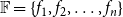
) propagating through the underlying network, we have four possible states for each node. We encode these states as 0, 1, 2, and 3, that is, we let
$\mathbb{C}_2$
) propagating through the underlying network, we have four possible states for each node. We encode these states as 0, 1, 2, and 3, that is, we let $\mathbb{B}$
= {0, 1, 2, 3}. The interpretation of these state values is shown in Table 1. An easy way to think of these states is to consider the 2-bit binary expansion of the state values 0 through 3. The least (most) significant bit indicates whether the node has been infected by
$\mathbb{B}$
= {0, 1, 2, 3}. The interpretation of these state values is shown in Table 1. An easy way to think of these states is to consider the 2-bit binary expansion of the state values 0 through 3. The least (most) significant bit indicates whether the node has been infected by $\mathbb{C}_1$
(
$\mathbb{C}_1$
( $\mathbb{C}_2$
).
$\mathbb{C}_2$
).
Table 1. Possible states for each node in the two contagion SyDS
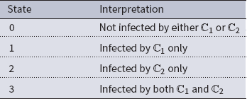
We assume that the system is progressive with respect to each of the contagions (Easley & Kleinberg Reference Easley and Kleinberg2010), that is, once a node is infected by a contagion, it remains infected by that contagion. Using this assumption, Figure 1 shows all the possible state transitions for each node.
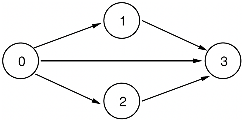
Figure 1. Possible state transitions for each node.
State transition rules: As stated earlier, each node v is associated with a local transition function $f_v$
that determines the next state of v given its current state and the states of its neighbors. Such a function may be deterministic or stochastic (e.g., SIR systems Hethcote Reference Hethcote2000). Here, we consider a class of deterministic functions called threshold functions.
$f_v$
that determines the next state of v given its current state and the states of its neighbors. Such a function may be deterministic or stochastic (e.g., SIR systems Hethcote Reference Hethcote2000). Here, we consider a class of deterministic functions called threshold functions.
A general form of local functions: We first discuss a very general (but somewhat complex) form of local functions for the propagation of two contagions in a network and then present a simpler form that will be used in the paper. In the general form, for each node v and for each of the five possible state transitions x to y (shown in Figure 1), there is a threshold value $\theta(v, x, y)$
. Let N(v,j) denote the number of neighbors of v in state j,
$\theta(v, x, y)$
. Let N(v,j) denote the number of neighbors of v in state j, $0 \leq j \leq 3$
. (If the state of node v is j, then v is also included in the count N(v,j).) For any node v, the rules for each possible state transition which collectively specify the local function
$0 \leq j \leq 3$
. (If the state of node v is j, then v is also included in the count N(v,j).) For any node v, the rules for each possible state transition which collectively specify the local function $f_v$
are shown in Table 2.
$f_v$
are shown in Table 2.
Table 2. Transition rules to specify the general form of local function $f_v$
at node v
$f_v$
at node v
We will briefly explain two of the state transition conditions as shown in Table 2. The explanations for the other transitions are similar. Consider the condition for the “ $0 \longrightarrow 1$
” transition. For this transition to occur at a node v, the number of neighbors of v in state 1 or state 3 must be at least
$0 \longrightarrow 1$
” transition. For this transition to occur at a node v, the number of neighbors of v in state 1 or state 3 must be at least $\theta(v,0,1)$
(i.e.,
$\theta(v,0,1)$
(i.e., $N(v,1)+ N(v,3) \geq \theta(v,0,1)$
) and the number of neighbors of v in state 2 or state 3 must be less than
$N(v,1)+ N(v,3) \geq \theta(v,0,1)$
) and the number of neighbors of v in state 2 or state 3 must be less than $\theta(v,0, 2)$
(i.e.,
$\theta(v,0, 2)$
(i.e., $N(v,2)+ N(v,3) < \theta(v,0,2)$
). Likewise, for the “
$N(v,2)+ N(v,3) < \theta(v,0,2)$
). Likewise, for the “ $1 \longrightarrow 3$
” transition to occur at v, the number of neighbors of v in state 2 or state 3 must be at least
$1 \longrightarrow 3$
” transition to occur at v, the number of neighbors of v in state 2 or state 3 must be at least $\theta(v,1,3)$
(i.e.,
$\theta(v,1,3)$
(i.e., $N(v,2)+ N(v,3) \geq \theta(v,1,3)$
).
$N(v,2)+ N(v,3) \geq \theta(v,1,3)$
).
The above general model is powerful as it allows the two contagions to interact. Many references have considered cooperating and competing contagions (e.g., Karrer & Newman Reference Karrer and Newman2011; Newman et al. 2013; Kumar et al. Reference Kumar, Verma, Singh and Cherifi2019). For example, if a node has already contracted $\mathbb{C}_1$
, it may be “easier” for it to contract
$\mathbb{C}_1$
, it may be “easier” for it to contract $\mathbb{C}_2$
. This can be modeled by choosing a low value for
$\mathbb{C}_2$
. This can be modeled by choosing a low value for $\theta(v,1,3)$
. However, the model is also complex since it requires the specification of five threshold values for each node. In this paper, we consider a simpler model which uses only two threshold values for each node. We now explain the simpler model.
$\theta(v,1,3)$
. However, the model is also complex since it requires the specification of five threshold values for each node. In this paper, we consider a simpler model which uses only two threshold values for each node. We now explain the simpler model.
A simpler form of local functions: In the simpler model, for each node v, we use two threshold values, denoted by $\theta(v,1)$
and
$\theta(v,1)$
and $\theta(v,2)$
. The parameter
$\theta(v,2)$
. The parameter $\theta(v,1)$
is used when v is in state 0 or state 2 (i.e., v has not contracted contagion
$\theta(v,1)$
is used when v is in state 0 or state 2 (i.e., v has not contracted contagion $\mathbb{C}_1$
); it specifies the minimum number of neighbors of v whose state is either 1 or 3 so that v can contract contagion
$\mathbb{C}_1$
); it specifies the minimum number of neighbors of v whose state is either 1 or 3 so that v can contract contagion $\mathbb{C}_1$
. Similarly,
$\mathbb{C}_1$
. Similarly, $\theta(v,2)$
specifies the minimum number of neighbors of v whose state is either 2 or 3 so that v can contract contagion
$\theta(v,2)$
specifies the minimum number of neighbors of v whose state is either 2 or 3 so that v can contract contagion $\mathbb{C}_2$
. Unlike the general model, the simpler model does not permit interactions between the two contagions. However, the simpler model facilitates the development of analytical and experimental results.
$\mathbb{C}_2$
. Unlike the general model, the simpler model does not permit interactions between the two contagions. However, the simpler model facilitates the development of analytical and experimental results.
2.2 Additional definitions concerning SyDSs
At any time $\tau$
, the configuration
$\tau$
, the configuration $\mathbb{C}$
of a SyDS is the n-vector
$\mathbb{C}$
of a SyDS is the n-vector $(s_1^{\tau}, s_2^{\tau}, \ldots, s_n^{\tau})$
, where
$(s_1^{\tau}, s_2^{\tau}, \ldots, s_n^{\tau})$
, where $s_i^{\tau} \in \mathbb{B}$
is the state of node
$s_i^{\tau} \in \mathbb{B}$
is the state of node $v_i$
at time
$v_i$
at time $\tau$
(
$\tau$
( $1 \leq i \leq n$
). Given a configuration
$1 \leq i \leq n$
). Given a configuration $\mathbb{C}$
, the state of a node v in
$\mathbb{C}$
, the state of a node v in $\mathbb{C}$
is denoted by
$\mathbb{C}$
is denoted by $\mathbb{C}(v)$
. In a SyDS, all nodes compute and update their next state synchronously. Other update disciplines (e.g., sequential updates) have also been considered in the literature (e.g., Mortveit & Reidys Reference Mortveit and Reidys2007; Barrett et al. Reference Barrett, Hunt, Marathe, Ravi, Rosenkrantz, Stearns and Thakur2007). Suppose a given SyDS transitions in one step from a configuration
$\mathbb{C}(v)$
. In a SyDS, all nodes compute and update their next state synchronously. Other update disciplines (e.g., sequential updates) have also been considered in the literature (e.g., Mortveit & Reidys Reference Mortveit and Reidys2007; Barrett et al. Reference Barrett, Hunt, Marathe, Ravi, Rosenkrantz, Stearns and Thakur2007). Suppose a given SyDS transitions in one step from a configuration $\mathbb{C'}$
to a configuration
$\mathbb{C'}$
to a configuration $\mathbb{C}$
. Then, we say that
$\mathbb{C}$
. Then, we say that $\mathbb{C}$
is the successor of
$\mathbb{C}$
is the successor of $\mathbb{C'}$
, and
$\mathbb{C'}$
, and $\mathbb{C'}$
is a predecessor of
$\mathbb{C'}$
is a predecessor of $\mathbb{C}$
. Since the SyDSs considered in this paper are deterministic, each configuration has a unique successor. However, a configuration may have zero or more predecessors. A configuration
$\mathbb{C}$
. Since the SyDSs considered in this paper are deterministic, each configuration has a unique successor. However, a configuration may have zero or more predecessors. A configuration $\mathbb{C}$
which is its own successor is called a fixed point. Thus, when a SyDS reaches a fixed point, no further state changes occur at any node.
$\mathbb{C}$
which is its own successor is called a fixed point. Thus, when a SyDS reaches a fixed point, no further state changes occur at any node.
Example: The underlying network of a SyDS in which two contagions are propagating under the simpler model discussed above is shown in Figure 2. For each node v, the two threshold values $\theta(v,1)$
and
$\theta(v,1)$
and $\theta(v,2)$
are both chosen as 1 in this example. Suppose the initial states of nodes
$\theta(v,2)$
are both chosen as 1 in this example. Suppose the initial states of nodes $v_1$
,
$v_1$
, $v_2$
,
$v_2$
, $v_3$
, and
$v_3$
, and $v_4$
are 1, 2, 0, and 0 respectively, that is, the initial configuration of the system is (1, 2, 0, 0). The local function
$v_4$
are 1, 2, 0, and 0 respectively, that is, the initial configuration of the system is (1, 2, 0, 0). The local function $f_1$
at
$f_1$
at $v_1$
is computed as follows. Since
$v_1$
is computed as follows. Since $v_1$
is in state 1, we need to check if it can contract contagion
$v_1$
is in state 1, we need to check if it can contract contagion $\mathbb{C}_2$
. Since
$\mathbb{C}_2$
. Since $\theta(v_1, 2)$
= 1 and
$\theta(v_1, 2)$
= 1 and $v_1$
has a neighbor (namely
$v_1$
has a neighbor (namely $v_2$
) in state 2,
$v_2$
) in state 2, $v_1$
will indeed contract contagion
$v_1$
will indeed contract contagion $\mathbb{C}_2$
. Therefore, the value of the local function
$\mathbb{C}_2$
. Therefore, the value of the local function $f_1$
is 3, that is, the next state of
$f_1$
is 3, that is, the next state of $v_1$
is 3. In a similar manner, it can be seen that the local functions
$v_1$
is 3. In a similar manner, it can be seen that the local functions $f_2$
and
$f_2$
and $f_3$
also evaluate to 3. For node
$f_3$
also evaluate to 3. For node $v_4$
, whose current state is 0, there is one neighbor (namely,
$v_4$
, whose current state is 0, there is one neighbor (namely, $v_2$
) whose state is 2. Therefore, the local function
$v_2$
) whose state is 2. Therefore, the local function $f_4$
evaluates to 2. Thus, the configuration of the system at time 1 is (3, 3, 3, 2). Since the system is progressive, the states of nodes
$f_4$
evaluates to 2. Thus, the configuration of the system at time 1 is (3, 3, 3, 2). Since the system is progressive, the states of nodes $v_1$
,
$v_1$
, $v_2$
, and
$v_2$
, and $v_3$
will continue to be 3 in subsequent time steps. However, the state of node
$v_3$
will continue to be 3 in subsequent time steps. However, the state of node $v_4$
changes to 3 at time step 2, since
$v_4$
changes to 3 at time step 2, since $v_4$
has a neighbor (namely,
$v_4$
has a neighbor (namely, $v_2$
) whose state at time step 1 is 3. Thus, the configuration of the system at the end of time step 2 is (3, 3, 3, 3). In other words, the sequence of configurations of the system at times 0, 1, and 2 is
$v_2$
) whose state at time step 1 is 3. Thus, the configuration of the system at the end of time step 2 is (3, 3, 3, 3). In other words, the sequence of configurations of the system at times 0, 1, and 2 is
 \begin{align*}(1, 2, 0, 0) \longrightarrow (3, 3, 3, 2) \longrightarrow (3, 3, 3, 3)\end{align*}
This sequence is shown in Figure 3, where the node colors red, green, blue, and brown indicate states 0, 1, 2, and 3 respectively. Once the system reaches the configuration (3, 3, 3, 3), no further state changes can occur. Thus, the configuration (3, 3, 3, 3) is a fixed point for the system. $\Box$
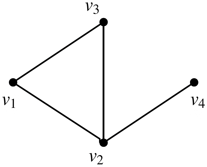
Figure 2. The underlying network of a SyDS with two contagions. For each node v, the threshold values $\theta(v,1)$
and
$\theta(v,1)$
and $\theta(v,2)$
are both 1.
$\theta(v,2)$
are both 1.
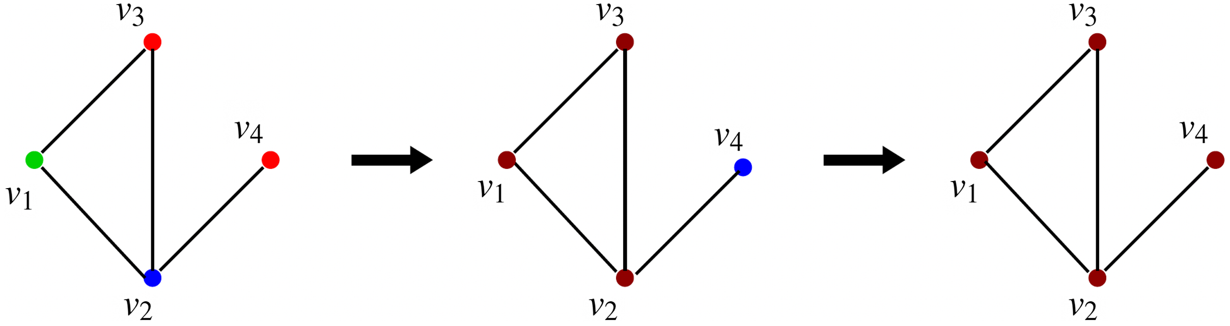
Figure 3. A sequence of configurations for the SyDS whose underlying graph is shown in Figure 2. Node colors red, green, blue and brown indicate states 0, 1, 2 and 3 respectively. The sequence of transitions shown above can also be represented as (1, 2, 0, 0) $\longrightarrow$
(3, 3, 3, 2)
$\longrightarrow$
(3, 3, 3, 2) $\longrightarrow$
(3, 3, 3, 3).
$\longrightarrow$
(3, 3, 3, 3).
This simple example illustrates the computations carried out by our simulation methods as discussed in Section 5. The only difference is that the simulation methods carry out these computations on much larger networks.
In this example, each of the nodes $v_3$
and
$v_3$
and $v_4$
had two new infections (one due to
$v_4$
had two new infections (one due to $\mathbb{C}_1$
and the other due to
$\mathbb{C}_1$
and the other due to $\mathbb{C}_2$
). Further, node
$\mathbb{C}_2$
). Further, node $v_1$
had one new infection (due to
$v_1$
had one new infection (due to $\mathbb{C}_2$
) and
$\mathbb{C}_2$
) and $v_2$
had one new infection (due to
$v_2$
had one new infection (due to $\mathbb{C}_1$
). Thus, the sequence of transitions shown in Figure 3 has a total of six new infections. Since the number of possible infections is
$\mathbb{C}_1$
). Thus, the sequence of transitions shown in Figure 3 has a total of six new infections. Since the number of possible infections is $2n=8$
for this example, and there are eight total infections (including the initial infections), the fraction of possible infections equals
$2n=8$
for this example, and there are eight total infections (including the initial infections), the fraction of possible infections equals $8/8=1$
.
$8/8=1$
.
In the above example, the SyDS reached a fixed point. Using our assumption that the system is progressive, one can show that every such SyDS reaches a fixed point.
Proposition 2.1. Every progressive SyDS under the two contagion model reaches a fixed point from every initial configuration
Proof: Consider any progressive SyDS on $\mathbb{B}$
=
$\mathbb{B}$
= $\{0,1,2,3\}$
. Let n denote the number of nodes in the underlying graph of the SyDS. In any transition from a configuration to a different configuration, at least one node changes state. Because the system is progressive, each node may change state at most twice: once from 0 to 1 (or 0 to 2) and then from 1 to 3 (or 2 to 3). Thus, after at most 2n transitions where the states of one or more nodes change, there can be no further state changes. In other words, the system reaches a fixed point after at most 2n transitions.
$\{0,1,2,3\}$
. Let n denote the number of nodes in the underlying graph of the SyDS. In any transition from a configuration to a different configuration, at least one node changes state. Because the system is progressive, each node may change state at most twice: once from 0 to 1 (or 0 to 2) and then from 1 to 3 (or 2 to 3). Thus, after at most 2n transitions where the states of one or more nodes change, there can be no further state changes. In other words, the system reaches a fixed point after at most 2n transitions.
3. Problem formulation, complexity results, and the SMC problem
3.1 Blocking problem for two contagions
The focus of this paper is on a method for containing the propagation of the two contagions by appropriately vaccinating a subset of nodes. Before defining the problem formally, we state the assumptions used in our formulation.
When a node is vaccinated for a certain contagion, the node cannot get infected by that contagion; as a consequence, such a node cannot propagate the corresponding contagion. For $i = 1,2$
, one can think of vaccinating a node v for a contagion
$i = 1,2$
, one can think of vaccinating a node v for a contagion $\mathbb{C}_i$
as increasing the threshold
$\mathbb{C}_i$
as increasing the threshold $\theta(v,i)$
of the node v to degree(v)+1 so that the number of neighbors of v that are infected by
$\theta(v,i)$
of the node v to degree(v)+1 so that the number of neighbors of v that are infected by $\mathbb{C}_i$
will always be less than
$\mathbb{C}_i$
will always be less than $\theta(v,i)$
. If a node v is vaccinated for both
$\theta(v,i)$
. If a node v is vaccinated for both $\mathbb{C}_1$
and
$\mathbb{C}_1$
and $\mathbb{C}_2$
, then it plays no role in propagating either contagion. In such a situation, one can think of the effect of vaccinating v as removing node v and all the edges incident on v from the network.
$\mathbb{C}_2$
, then it plays no role in propagating either contagion. In such a situation, one can think of the effect of vaccinating v as removing node v and all the edges incident on v from the network.
The optimization problem studied in this paper is a generalization of a problem studied in Kuhlman et al. (Reference Kuhlman, Kumar, Marathe, Ravi and Rosenkrantz2015) for a single contagion. This problem deals with choosing a small set of nodes to vaccinate so that the total number of new infections when the system reaches a fixed point is a minimum. Given a set C of nodes to be vaccinated, a vaccination scheme specifies for each node $w \in C$
, whether w is vaccinated against
$w \in C$
, whether w is vaccinated against $\mathbb{C}_1$
,
$\mathbb{C}_1$
, $\mathbb{C}_2$
, or both. The total number of vaccinations used by a vaccination scheme for a set of nodes C is the sum
$\mathbb{C}_2$
, or both. The total number of vaccinations used by a vaccination scheme for a set of nodes C is the sum $N_1 + N_2$
, where
$N_1 + N_2$
, where $N_i$
is the number of nodes vaccinated against
$N_i$
is the number of nodes vaccinated against $\mathbb{C}_i$
,
$\mathbb{C}_i$
, $i = 1, 2$
. Note that if a node w is vaccinated against both
$i = 1, 2$
. Note that if a node w is vaccinated against both $\mathbb{C}_1$
and
$\mathbb{C}_1$
and $\mathbb{C}_2$
, then it is included in both the counts
$\mathbb{C}_2$
, then it is included in both the counts $N_1$
and
$N_1$
and $N_2$
. Given a budget
$N_2$
. Given a budget $\beta$
on the number of vaccinations, the chosen vaccination scheme must ensure that
$\beta$
on the number of vaccinations, the chosen vaccination scheme must ensure that $\beta \leq N_1 + N_2$
. Also, after a vaccination scheme is chosen and the contagions spread through the network, the number of new infections is computed as follows. For
$\beta \leq N_1 + N_2$
. Also, after a vaccination scheme is chosen and the contagions spread through the network, the number of new infections is computed as follows. For $0 \leq i \leq j \leq 3$
, let
$0 \leq i \leq j \leq 3$
, let $\Gamma_{ij}$
denote the set of nodes whose initial state is i and whose final state (when the system reaches a fixed point) is j. Then, the number of new infections is given by
$\Gamma_{ij}$
denote the set of nodes whose initial state is i and whose final state (when the system reaches a fixed point) is j. Then, the number of new infections is given by $|\Gamma_{01}| + |\Gamma_{02}| + |\Gamma_{13}| + |\Gamma_{23}|+ 2 \times |\Gamma_{03}|$
; the reason for the factor 2 in the last term of this expression is that nodes that start in state 0 and end in state 3 suffer two infections. We can now provide a formal statement of the main optimization problem considered in this paper.
$|\Gamma_{01}| + |\Gamma_{02}| + |\Gamma_{13}| + |\Gamma_{23}|+ 2 \times |\Gamma_{03}|$
; the reason for the factor 2 in the last term of this expression is that nodes that start in state 0 and end in state 3 suffer two infections. We can now provide a formal statement of the main optimization problem considered in this paper.
Vaccination Scheme to Minimize the Total Number of New Infections (VS-MTNNI)
Given: A social network represented by the SyDS $\mathsf{S}$
=
$\mathsf{S}$
= $(G, \mathbb{F})$
over
$(G, \mathbb{F})$
over $\mathbb{B}$
= {0, 1, 2, 3}, with each local function
$\mathbb{B}$
= {0, 1, 2, 3}, with each local function $f_v \in \mathbb{F}$
at node v represented by two threshold values
$f_v \in \mathbb{F}$
at node v represented by two threshold values $\theta(v,1)$
and
$\theta(v,1)$
and $\theta(v,2)$
; the set I of seed nodes which are initially infected (i.e., the state of each node in I is from {1,2,3}); an upper bound
$\theta(v,2)$
; the set I of seed nodes which are initially infected (i.e., the state of each node in I is from {1,2,3}); an upper bound $\beta$
on the total number of vaccinations.
$\beta$
on the total number of vaccinations.
Requirement: A set $C \subseteq V$
of nodes to be vaccinated and a vaccination scheme for C so that (i) the total number of vaccinations is at most
$C \subseteq V$
of nodes to be vaccinated and a vaccination scheme for C so that (i) the total number of vaccinations is at most $\beta$
and (ii) among all subsets of V which can be vaccinated to satisfy (i), the set C and the chosen vaccination scheme lead to the smallest number of new infections.
$\beta$
and (ii) among all subsets of V which can be vaccinated to satisfy (i), the set C and the chosen vaccination scheme lead to the smallest number of new infections.
To show the computationally intractability of Vaccination Scheme to Minimize the Total Number of New Infections VS-MTNNI, we use the following problem and result from Kuhlman et al. (Reference Kuhlman, Kumar, Marathe, Ravi and Rosenkrantz2015).
Smallest Critical Set to Minimize the number of Newly Affected nodes (SCS-MNA)
Given: A SyDS represented by a graph G(V,E) through which a single contagion is propagating, a threshold value $\theta(v)$
for each node v, a set
$\theta(v)$
for each node v, a set $I \subseteq V$
of initially infected nodes, a vaccination budget
$I \subseteq V$
of initially infected nodes, a vaccination budget $\beta$
, and an upper bound Q on the number of new infections.
$\beta$
, and an upper bound Q on the number of new infections.
Requirement: A subset $C \subseteq V$
such that
$C \subseteq V$
such that $|C| \leq \beta$
and after vaccinating the nodes in C, the number of new infections in G is at most Q.
$|C| \leq \beta$
and after vaccinating the nodes in C, the number of new infections in G is at most Q.
The following result is from Kuhlman et al. (Reference Kuhlman, Kumar, Marathe, Ravi and Rosenkrantz2015). In stating this result, we use the following definition. An algorithm for the Smallest Critical Set to Minimize the number of Newly Affected nodes (SCS-MNA) problem provides a factor $\rho$
approximation if for every instance of the problem, the number of new infections is at most
$\rho$
approximation if for every instance of the problem, the number of new infections is at most $\rho Q^*$
, where
$\rho Q^*$
, where $Q^*$
is the minimum number of new infections.
$Q^*$
is the minimum number of new infections.
Theorem 3.1. The SCS-MNA problem is NP-hard even when each threshold value is 2. Further, if the vaccination budget cannot be violated, the problem cannot be efficiently approximated to within any factor $\rho \geq 1$
, unless P = NP.
$\rho \geq 1$
, unless P = NP.
We now show that the result of Theorem 3.1 also holds for the VS-MTNNI problem.
Theorem 3.2. The VS-MTNNI problem is NP-hard even when each threshold value is 2. Further, if the vaccination budget cannot be violated, the problem cannot be approximated to within any factor $\rho \geq 1$
, unless P = NP.
$\rho \geq 1$
, unless P = NP.
Proof: The SCS-MNA problem can be reduced in a straightforward manner to the VS-MTNNI problem as follows. Let an instance of SCS-MNA be given by a graph G(V,E), a subset $I \subseteq V$
of initially infected nodes (for the only contagion), a vaccination budget
$I \subseteq V$
of initially infected nodes (for the only contagion), a vaccination budget $\beta$
, and an upper bound Q on the number of new infections. From the graph G(V,E) of the SCS-MNA instance, we create a new graph G’(V’,E) by adding a new node v to V such that v has no incident edges (i.e.,
$\beta$
, and an upper bound Q on the number of new infections. From the graph G(V,E) of the SCS-MNA instance, we create a new graph G’(V’,E) by adding a new node v to V such that v has no incident edges (i.e., $\mathrm{degree}(v) = 0$
). In the VS-MTNNI instance, the initial state of each node in I is chosen as 1 and the initial state of the new node v is chosen as 2. The two threshold values for each node in G’ are chosen as 2. The bound on the number of new infections in G’ is set to Q, the corresponding value for G. Clearly, this construction can be carried out in polynomial time. Further, the construction ensures that only
$\mathrm{degree}(v) = 0$
). In the VS-MTNNI instance, the initial state of each node in I is chosen as 1 and the initial state of the new node v is chosen as 2. The two threshold values for each node in G’ are chosen as 2. The bound on the number of new infections in G’ is set to Q, the corresponding value for G. Clearly, this construction can be carried out in polynomial time. Further, the construction ensures that only $\mathbb{C}_1$
can spread in the SyDS represented by G’.
$\mathbb{C}_1$
can spread in the SyDS represented by G’.
Suppose there is a solution to the SCS-MNA instance for G. The solution to the VS-MTNNI instance is obtained from the solution to the SCS-MNA instance by using the budget $\beta$
to block contagion
$\beta$
to block contagion $\mathbb{C}_1$
in G’. Since only
$\mathbb{C}_1$
in G’. Since only $\mathbb{C}_1$
can spread in G’, this vaccination scheme ensures that the number of new infections in G’ is also at most Q. Similarly, if there is a solution to the VS-MTNNI instance, the vaccination scheme used in this solution is also a valid solution to the SCS-MNA instance for G.
$\mathbb{C}_1$
can spread in G’, this vaccination scheme ensures that the number of new infections in G’ is also at most Q. Similarly, if there is a solution to the VS-MTNNI instance, the vaccination scheme used in this solution is also a valid solution to the SCS-MNA instance for G.
Therefore, any vaccination scheme for G’ which vaccinates at most $\beta$
that causes at most Q new infections is also a solution to the SCS-MNA instance and vice versa. This completes our proof of Theorem 3.2. ■
$\beta$
that causes at most Q new infections is also a solution to the SCS-MNA instance and vice versa. This completes our proof of Theorem 3.2. ■
3.2 SMC problem
In Section 4, we will present a heuristic algorithm (which we refer to as MCICH-SMC) for the VS-MTNNI problem. This heuristic relies on known methods for solving a generalized version of the MSC problem (Garey & Johnson Reference Garey and Johnson1979). This generalized version of MSC is called SMC (Vazirani Reference Vazirani2001). An approach based on SMC was used in Kuhlman et al. (Reference Kuhlman, Kumar, Marathe, Ravi and Rosenkrantz2015) to obtain a heuristic for blocking a single contagion. We now present the definition of the SMC problem and two known methods for solving it. We state SMC as a constrained maximization problem, since that version can be directly used in our heuristic for the VS-MTNNI problem.
Set Multicover (SMC)
Given: A universe $U = \{u_1, u_2, \ldots, u_n\}$
of n elements, a collection
$U = \{u_1, u_2, \ldots, u_n\}$
of n elements, a collection $C = \{C_1, C_2, \ldots, C_m\}$
of subsets of U, an integer (coverage requirement)
$C = \{C_1, C_2, \ldots, C_m\}$
of subsets of U, an integer (coverage requirement) $r_i \geq 1$
for each
$r_i \geq 1$
for each $u_i \in U$
,
$u_i \in U$
, $1 \leq i \leq n$
, a budget
$1 \leq i \leq n$
, a budget $\beta \leq m$
.
$\beta \leq m$
.
Required: A collection $C' \subseteq C$
such that
$C' \subseteq C$
such that $|C'| \leq \beta$
and the size of the set U’ given by
$|C'| \leq \beta$
and the size of the set U’ given by $U' = \{u_i \in U \::\:$
the number of sets in C’ that contain
$U' = \{u_i \in U \::\:$
the number of sets in C’ that contain $u_i$
is
$u_i$
is $~\geq~$ $r_i\}$
is maximized.
$r_i\}$
is maximized.
In the above definition, U’ represents the subset of elements whose coverage requirement is satisfied by the chosen subcollection C’. Note that in SMC, if $r_i = 1$
,
$r_i = 1$
, $1 \leq i \leq n$
, and
$1 \leq i \leq n$
, and $|U'| = n$
, then we have the usual MSC problem (Garey & Johnson Reference Garey and Johnson1979). Thus, SMC is also a computationally intractable problem.
$|U'| = n$
, then we have the usual MSC problem (Garey & Johnson Reference Garey and Johnson1979). Thus, SMC is also a computationally intractable problem.
We use two known approaches to deal with the SMC problem. One approach is to solve the problem optimally using an ILP formulation. The other approach is to use an efficient greedy heuristic for the problem. These two approaches, which are used in our experimental study, are discussed below.
An ILP Formulation for SMC: The following ILP for SMC is based on the description in Vazirani (Reference Vazirani2001).
a. Variables: Given an SMC instance where there are m sets and n elements, our ILP formulation uses $m+n$
variables as discussed below:
$m+n$
variables as discussed below:
-
i. For each set $C_j$
, we have a variable
$y_j$
which takes on a value from
$\{0,1\}$
,
$1 \leq j \leq m$
. (If
$y_j = 1$
, then set
$C_j$
is chosen in the cover; otherwise,
$C_j$
is not chosen.)
$C_j$
, we have a variable
$y_j$
which takes on a value from
$\{0,1\}$
,
$1 \leq j \leq m$
. (If
$y_j = 1$
, then set
$C_j$
is chosen in the cover; otherwise,
$C_j$
is not chosen.) -
ii. For each element
$u_i$
, we have a variable
$x_i$
which also takes on a value from
$\{0,1\}$
,
$1 \leq i \leq n$
. (If
$x_i = 1$
, then the coverage requirement for element
$u_i$
is satisfied; otherwise, the coverage requirement is not satisfied.)


b. Objective function: We need to maximize the number of elements whose coverage requirement is satisfied. So, the objective is
Maximize $\displaystyle{\sum_{i=1}^{n} x_i}$
.
$\displaystyle{\sum_{i=1}^{n} x_i}$
.
c. Constraints:
-
a. The total number of subsets chosen must be at most
$\beta$
. This constraint is
\begin{align*}\displaystyle{\sum_{j=1}^{m} y_j ~\leq~ \beta}.\end{align*}
-
b. We need to check whether the chosen collection of sets satisfies the coverage requirement for each element
$u_i$
. Constraints must be chosen so that if the coverage requirement for element
$u_i$
is met, then
$x_i = 1$
; otherwise,
$x_i = 0$
. This can be done as follows. For element
$u_i$
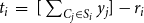
, let
$S_i \subseteq C$
be the collection of subsets each of which has
$u_i$
as an element. Let
$t_i ~=~ [\sum_{C_j \in S_i} y_j] - r_i$
. In this expression for
$t_i$
, the summation gives the number of chosen sets that have
$u_i$
as an element. Therefore, if
$t_i \geq 0$
, then the coverage requirement for
$u_i$
is satisfied; otherwise, the coverage requirement for
$u_i$
is not satisfied. We need to use this expression to set
$x_i$
appropriately. This can be done using the following two (linear) constraints. (Recall that m is the number of sets in the collection C.)


 \begin{align*}\displaystyle{m\,x_i ~~\geq~~ \left[ \sum_{C_j \in S_i} y_j \right] - r_i + 1} ~~~\textrm{and}~~~\displaystyle{m\,x_i ~~\leq~~ \left[ \sum_{C_j \in S_i} y_j \right] - r_i + m}.\end{align*}
This completes our ILP formulation for SMC.
A Greedy Heuristic for SMC: This iterative heuristic for SMC is similar to the greedy heuristic for the MSC problem (Vazirani Reference Vazirani2001). In each iteration, it picks a set which covers the largest number of elements whose coverage requirement has not yet been met. This algorithm returns a collection of $\beta$
subsets from C. Subject to this constraint, it tries to find a solution that satisfies the coverage requirements for as many elements as possible. An outline for this method is shown in Algorithm 1. In Section 4, we discuss how this heuristic is useful in developing our heuristic for the VS-MTNNI problem.
$\beta$
subsets from C. Subject to this constraint, it tries to find a solution that satisfies the coverage requirements for as many elements as possible. An outline for this method is shown in Algorithm 1. In Section 4, we discuss how this heuristic is useful in developing our heuristic for the VS-MTNNI problem.
Algorithm 1: Greedy Heuristic for the Set Multicover Problem

4. Approaches for solving the blocking problem
4.1 Overview
Theorem 3.2 points out that, in the worst-case, even obtaining an efficient approximation algorithm with a provable performance guarantee for the VS-MTNNI problem is computationally intractable. In this section, we now discuss two approaches for solving the VS-MTNNI problem in practice. The first approach develops an ILP formulation for obtaining optimal solutions. Since known algorithms for solving ILPs take exponential time in the worst-case, this approach is suitable for small networks. For larger networks, we present an efficient heuristic to obtain good (but not necessarily optimal) solutions in practice.
4.2 Obtaining optimal solutions: An ILP formulation for VS-MTNNI
We first discuss the notation used to develop our ILP formulation for the VS-MTNNI problem. The n nodes of the underlying network are denoted by $v_1$
,
$v_1$
, $v_2$
,
$v_2$
, $\ldots$
,
$\ldots$
, $v_n$
. Each node
$v_n$
. Each node $v_i$
has two threshold values denoted by
$v_i$
has two threshold values denoted by $\theta(v_i,1)$
and
$\theta(v_i,1)$
and $\theta(v_i,2)$
. We assume that all threshold values are
$\theta(v_i,2)$
. We assume that all threshold values are $\geq 1$
. The set of neighbors of node
$\geq 1$
. The set of neighbors of node $v_i$
is denoted by
$v_i$
is denoted by $\mathbb{N}_i$
and the degree of node
$\mathbb{N}_i$
and the degree of node $v_i$
is denoted by
$v_i$
is denoted by $d_i$
,
$d_i$
, $1 \leq i \leq n$
. (Thus,
$1 \leq i \leq n$
. (Thus, $d_i = |\mathbb{N}_i|$
.) The set of initially infected nodes (i.e., the seed set) is denoted by
$d_i = |\mathbb{N}_i|$
.) The set of initially infected nodes (i.e., the seed set) is denoted by $\mathbb{S}$
. The number of infections in
$\mathbb{S}$
. The number of infections in $\mathbb{S}$
is
$\mathbb{S}$
is $N_1 + N_2$
, where
$N_1 + N_2$
, where $N_j$
denotes the number of nodes infected by
$N_j$
denotes the number of nodes infected by $\mathbb{C}_j$
,
$\mathbb{C}_j$
, $j = 1, 2$
. Thus, if a node is infected by both
$j = 1, 2$
. Thus, if a node is infected by both $\mathbb{C}_1$
and
$\mathbb{C}_1$
and $\mathbb{C}_2$
, it is counted twice in the number of infections. The budget on the number of nodes that can be blocked is denoted by
$\mathbb{C}_2$
, it is counted twice in the number of infections. The budget on the number of nodes that can be blocked is denoted by $\beta$
. We are now ready to present the ILP formulation.
$\beta$
. We are now ready to present the ILP formulation.
a. Variables: For each node $v_i$
,
$v_i$
, $1 \leq i \leq n$
, we have six {0,1}-valued variables denoted by
$1 \leq i \leq n$
, we have six {0,1}-valued variables denoted by $x_{i,j}$
,
$x_{i,j}$
, $y_{i,j}$
and
$y_{i,j}$
and $z_{i,j}$
,
$z_{i,j}$
, $j = 1, 2$
. (Thus, the total number of variables in the ILP formulation is 6n.) The significance of these variables is as follows:
$j = 1, 2$
. (Thus, the total number of variables in the ILP formulation is 6n.) The significance of these variables is as follows:
-
i. Variable
$x_{i,j}$
is 1 iff
$v_i$
is susceptible to
$\mathbb{C}_j$
(i.e.,
$v_i$
does not get infected by
$\mathbb{C}_j$
after blocking). -
ii. Variable
$y_{i,j}$
is 1 iff
$v_i$
is infected by
$\mathbb{C}_j$
. -
iii. Variable
$z_{i,j}$
is 1 iff
$v_i$
is blocked for
$\mathbb{C}_j$
(i.e., it cannot get infected by
$\mathbb{C}_j$
).


b. Objective function: We want to minimize the number of new infections. So,
Minimize $\displaystyle{\sum_{i=1}^{n} (y_{i,1} + y_{i,2}) ~-~ \gamma}$
,
$\displaystyle{\sum_{i=1}^{n} (y_{i,1} + y_{i,2}) ~-~ \gamma}$
,
where $\gamma$
is the number of initial infections. (We note that the number of initial infections
$\gamma$
is the number of initial infections. (We note that the number of initial infections $\gamma$
can be computed from the seed set
$\gamma$
can be computed from the seed set $\mathbb{S}$
.)
$\mathbb{S}$
.)
c. Constraints:
-
1. For each node
$v_i$
and each contagion
$\mathbb{C}_j$
, there are three possibilities:
$v_i$
may be susceptible or infected or blocked. Therefore, we have
$x_{i,j} + y_{i,j} + z_{i,j} ~=~ 1,~~ 1 \leq i \leq n ~~\mathrm{and}~~ j = 1,2$
. -
2. For each node
$v_i \in \mathbb{S}$
, if it is infected by
$\mathbb{C}_j$
, then
$y_{i,j} = 1$
. -
3. At the end of the simulation, if a node
$v_i$
is not infected by
$\mathbb{C}_j$
, the following constraint must hold for
$1 \leq i \leq n$
and
$j = 1, 2$
:
$d_i\,x_{i,j} + \sum_{v_p \in {\mathbb{N}_i}} y_{p,j} ~~\leq~~ d_i + \theta(v_i, j) -1$
, where
$d_i$
is the degree of
$v_i$
and
$\mathbb{N}_i$
is the set of neighbors of
$v_i$
. Reason: Suppose
$x_{i,j}$
is 1 at the end of the simulation. Then, the number of neighbors of
$v_i$
who are infected by
$\mathbb{C}_j$
must be less than the threshold
$\theta(v_i, j)$
. If
$x_{i,j} = 0$
, the above constraint holds trivially. -
4. Budget constraint: The total number of nodes blocked for either or both of the contagions should be at most
$\beta$
. This gives rise to the following constraint:


 $\displaystyle{\sum_{i=1}^{n} \sum_{j=1}^{2} z_{i,j} ~\leq~ \beta}$
.
$\displaystyle{\sum_{i=1}^{n} \sum_{j=1}^{2} z_{i,j} ~\leq~ \beta}$
.
This completes the ILP formulation for the VS-MTNNI problem. One advantage of this ILP formulation is that it can be generalized in a straightforward manner to handle any number $\sigma \geq 2$
of contagions as follows. The generalization uses a total of
$\sigma \geq 2$
of contagions as follows. The generalization uses a total of $3\sigma n$
variables (i.e.,
$3\sigma n$
variables (i.e., $x_{i,j}$
,
$x_{i,j}$
, $y_{i,j}$
,
$y_{i,j}$
, $z_{i,j}$
,
$z_{i,j}$
, $1 \leq i \leq n$
and
$1 \leq i \leq n$
and $1 \leq j \leq \sigma$
). In each of the above constraints, the range of the index j would be
$1 \leq j \leq \sigma$
). In each of the above constraints, the range of the index j would be $j = 1, 2, \ldots, \sigma$
.
$j = 1, 2, \ldots, \sigma$
.
4.3 A heuristic for VS-MTNNI based on SMC
In this section, we will discuss a new heuristic called MCICH-SMC for the VS-MTNNI problem. The basic idea is to solve a suitable SMC problem to identify a subset of nodes that are activated at time t to set as blocking nodes, such that no nodes will be activated at time $t+1$
. If this is accomplished, then the contagion is halted at t, and our goal is achieved.
$t+1$
. If this is accomplished, then the contagion is halted at t, and our goal is achieved.
A key idea, as noted in Kuhlman et al. (Reference Kuhlman, Kumar, Marathe, Ravi and Rosenkrantz2015) for the single-contagion case, is that any node $v_i$
that is activated at time
$v_i$
that is activated at time $t+1$
does so because it receives influence from nodes activated at time t, for otherwise,
$t+1$
does so because it receives influence from nodes activated at time t, for otherwise, $v_i$
would have activated at an earlier time. We now explain through an example how the SMC problem arises naturally in the context of blocking contagions.
$v_i$
would have activated at an earlier time. We now explain through an example how the SMC problem arises naturally in the context of blocking contagions.
Example: Figure 4 provides an example that highlights the key features of MCICH-SMC. Activated nodes are in green and inactive nodes are in red. The sets $S_t$
and
$S_t$
and $S_{t+1}$
are the sets of nodes that are newly activated at times t and
$S_{t+1}$
are the sets of nodes that are newly activated at times t and $t+1$
, respectively, for one contagion. With no blocking, these nodes are green. The method identifies a small number of nodes in
$t+1$
, respectively, for one contagion. With no blocking, these nodes are green. The method identifies a small number of nodes in $S_t$
to make red (i.e., to block) so that all nodes in
$S_t$
to make red (i.e., to block) so that all nodes in $S_{t+1}$
turn red. There are three and four activated nodes, respectively, in sets
$S_{t+1}$
turn red. There are three and four activated nodes, respectively, in sets $S_t$
and
$S_t$
and $S_{t+1}$
. The nodes at time t that assist in activating nodes at time
$S_{t+1}$
. The nodes at time t that assist in activating nodes at time $t+1$
are shown by green solid arrows. The numbers of neighbors that have activated each
$t+1$
are shown by green solid arrows. The numbers of neighbors that have activated each $v_i$
in
$v_i$
in $S_{t+1}$
are shown as
$S_{t+1}$
are shown as $\eta_1$
values to the right of each node, and the values are 3 and 4. (Some of these nodes are from levels that precede
$\eta_1$
values to the right of each node, and the values are 3 and 4. (Some of these nodes are from levels that precede $S_t$
.) These values of
$S_t$
.) These values of $\eta_1$
must be decreased to
$\eta_1$
must be decreased to $\eta_1 < \theta$
in order for the nodes in
$\eta_1 < \theta$
in order for the nodes in $S_{t+1}$
to not get activated. In the SMC instance constructed for
$S_{t+1}$
to not get activated. In the SMC instance constructed for $S_t$
and
$S_t$
and $S_{t+1}$
, one set is constructed for each node v in
$S_{t+1}$
, one set is constructed for each node v in $S_t$
, and the elements of the set are the neighbors of v in
$S_t$
, and the elements of the set are the neighbors of v in $S_{t+1}$
. The required amount of decrease represents the coverage requirement for each element in the SMC constructed for
$S_{t+1}$
. The required amount of decrease represents the coverage requirement for each element in the SMC constructed for $S_t$
and
$S_t$
and $S_{t+1}$
. We can now discuss how the greedy algorithm for SMC works for this example. In step 1 (middle panel),
$S_{t+1}$
. We can now discuss how the greedy algorithm for SMC works for this example. In step 1 (middle panel), $v_9 \in S_t$
is selected as the first blocking node because it has the most edges to nodes in
$v_9 \in S_t$
is selected as the first blocking node because it has the most edges to nodes in $S_{t+1}$
. Its color changes to red (the inactive state). The edges from
$S_{t+1}$
. Its color changes to red (the inactive state). The edges from $v_9$
are no longer active and are shown in dashed red. This reduces by 1 the
$v_9$
are no longer active and are shown in dashed red. This reduces by 1 the $\eta_1$
values for
$\eta_1$
values for $v_{14}$
,
$v_{14}$
, $v_{22}$
and
$v_{22}$
and $v_{39}$
, such that now
$v_{39}$
, such that now $\eta_1 < \theta$
for
$\eta_1 < \theta$
for $v_{22}$
and
$v_{22}$
and $v_{39}$
, and hence they change color to red. For
$v_{39}$
, and hence they change color to red. For $v_{14}$
,
$v_{14}$
, $\eta_1 = \theta$
, so it is still activated. Now, in the center panel, the activated node in
$\eta_1 = \theta$
, so it is still activated. Now, in the center panel, the activated node in $S_t$
that has the most remaining edges to activated nodes in
$S_t$
that has the most remaining edges to activated nodes in $S_{t+1}$
is
$S_{t+1}$
is $v_7$
, and this node is selected as the next blocking node, which occurs at step 2 (right panel). Hence,
$v_7$
, and this node is selected as the next blocking node, which occurs at step 2 (right panel). Hence, $v_7$
is red in the right panel, and it reduces by 1 the
$v_7$
is red in the right panel, and it reduces by 1 the $\eta_1$
values of
$\eta_1$
values of $v_6, v_{14} \in S_{t+1}$
such that for each of these two nodes
$v_6, v_{14} \in S_{t+1}$
such that for each of these two nodes $\eta_1 < \theta$
. Hence, they are colored red. In summary, by selecting as blocking nodes
$\eta_1 < \theta$
. Hence, they are colored red. In summary, by selecting as blocking nodes $v_7, v_9 \in S_t$
at time t, no nodes are activated at time
$v_7, v_9 \in S_t$
at time t, no nodes are activated at time $t+1$
, and the contagion is halted. Thus, in this example, there are two nodes, namely
$t+1$
, and the contagion is halted. Thus, in this example, there are two nodes, namely $v_7, v_9 \in S_t$
that are identified as blocking nodes, that is,
$v_7, v_9 \in S_t$
that are identified as blocking nodes, that is, $B=\{v_7, v_9\} \subset S_t$
.
$B=\{v_7, v_9\} \subset S_t$
. $\Box$

Figure 4. Illustration of the MCICH-SMC steps in selecting blocking nodes for a contagion. The panel on the left shows the sets $S_t$
and
$S_t$
and $S_{t+1}$
of newly activated nodes (in green) at times t and
$S_{t+1}$
of newly activated nodes (in green) at times t and $(t+1) > 1$
, respectively, from simulation output (with no blocking). All nodes
$(t+1) > 1$
, respectively, from simulation output (with no blocking). All nodes $v_i$
have
$v_i$
have $\theta=3$
. There are 3 and 4 newly activated nodes, respectively in
$\theta=3$
. There are 3 and 4 newly activated nodes, respectively in $S_t$
and
$S_t$
and $S_{t+1}$
. The numbers of neighbors that have activated each
$S_{t+1}$
. The numbers of neighbors that have activated each $v_i$
in
$v_i$
in $S_{t+1}$
(some of which are from infected sets before time t) are shown as
$S_{t+1}$
(some of which are from infected sets before time t) are shown as $\eta_1$
values to the right of each node.
$\eta_1$
values to the right of each node.
The algorithm for the MCICH-SMC is presented in Algorithm alg:coveringbm2. (For the sake of completeness, Part (B) of the algorithm also includes the steps of the greedy heuristic for SMC.) The algorithm considers one contagion at a time and computes the set B of blocking nodes using one simulation iteration, which is running the contagion propagation model using a set A of activated seed nodes at $t=0$
through a specified maximum time
$t=0$
through a specified maximum time $t_{\max}$
. Thus, with two contagions, the algorithm must be run twice, once for each contagion.
$t_{\max}$
. Thus, with two contagions, the algorithm must be run twice, once for each contagion.
Budget Allocation Between the Contagions: In generating all the blocking performance results in this paper (except for the ones in Section 5.3.9), the blocking budget $\beta$
was allocated between the two contagions using the proportion of nodes infected by contagions
$\beta$
was allocated between the two contagions using the proportion of nodes infected by contagions $\mathbb{C}_1$
and
$\mathbb{C}_1$
and $\mathbb{C}_2$
when there is no blocking. More precisely, suppose
$\mathbb{C}_2$
when there is no blocking. More precisely, suppose $n_1$
and
$n_1$
and $n_2$
denote the total number of infected nodes by
$n_2$
denote the total number of infected nodes by $\mathbb{C}_1$
and
$\mathbb{C}_1$
and $\mathbb{C}_2$
, respectively, in the absence of any blocking. We use
$\mathbb{C}_2$
, respectively, in the absence of any blocking. We use $n_1/(n_1+n_2)$
fraction of the budget for blocking
$n_1/(n_1+n_2)$
fraction of the budget for blocking $\mathbb{C}_1$
and the remaining budget for
$\mathbb{C}_1$
and the remaining budget for $\mathbb{C}_2$
. If the algorithm consumes less than the allocated budget for blocking
$\mathbb{C}_2$
. If the algorithm consumes less than the allocated budget for blocking $\mathbb{C}_1$
, the remaining allocation is used to increase the budget for
$\mathbb{C}_1$
, the remaining allocation is used to increase the budget for $\mathbb{C}_2$
. A discussion of the sensitivity of our approach for different budget allocations between the contagions is provided in Section 5.3.9.
$\mathbb{C}_2$
. A discussion of the sensitivity of our approach for different budget allocations between the contagions is provided in Section 5.3.9.
Variants of MCICH-SMC Used in Our Experiments: Our experiments with MCICH-SMC (discussed in Section 5) consider several variants of the heuristic. We describe these variants below.
a. The variants MCICH-SMC-Greedy and MCICH-SMC-ILP use, respectively, the greedy algorithm and the ILP for solving the SMC instances that arise during the execution of MCICH-SMC outlined in Algorithm 2.
Algorithm 2: Steps of the node blocking algorithm MCICH-SMC.

b. To understand the effect of the time parameter, we consider three variants of MCICH-SMC-ILP called MCICH-SMC-ILP-Low-Time, MCICH-SMC-ILP-Moderate-Time, and MCICH-SMC-ILP-High-Time. These three variants are assigned wall clock time limits of 120 seconds (or 2 minutes), 28,800 seconds (or 8 hours), and 521,700 seconds (about 6 days), respectively.
c. To understand the usefulness of MCICH-SMC in flattening the epidemic curve (see Section 5.3.7), we consider two variants of MCICH-SMC-Greedy, called “Before-Peak” and “Unconstrained,” respectively. The “Before-Peak” variant is required to pick the blocking nodes for each contagion at some time step before the number of infections for that contagion reaches its peak value, while the “Unconstrained” variant may pick the blocking nodes at any time step.
4.4 Two simple baselines for comparison purposes
Our experimental results also compare the performance of our main heuristic algorithm MCICH-SMC with two simple baseline approaches. These baseline methods are as follows.
a. Random Heuristic. For a given budget $\beta_i$
on the number of blocking nodes per contagion, select
$\beta_i$
on the number of blocking nodes per contagion, select $\beta_i$
nodes from among all nodes, uniformly at random.
$\beta_i$
nodes from among all nodes, uniformly at random.
b. High-Degree Heuristic. For a given budget $\beta_i$
on the number of blocking nodes per contagion, select the
$\beta_i$
on the number of blocking nodes per contagion, select the $\beta_i$
nodes with the largest degrees (breaking ties arbitrarily).
$\beta_i$
nodes with the largest degrees (breaking ties arbitrarily).
4.5 Summary of solution approaches
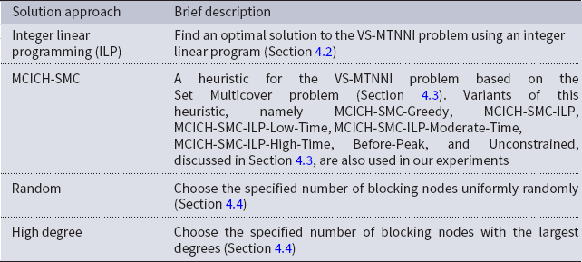
A summary of our main solution approaches for the VS-MTNNI problem discussed in this section is given in Table 3. Results from our experiments that compare the performance of these solution approaches are presented in Section 5.
Table 3. Table summarizing our solution approaches for the VS-MTNNI problem
5. Experimental results
5.1 Overview
In this section, we provide the networks tested, descriptions of the key elements of the analysis process and simulation, and results of the contagion blocking numerical experiments. Throughout this section, we use the words “activated” and “infected” as synonyms.
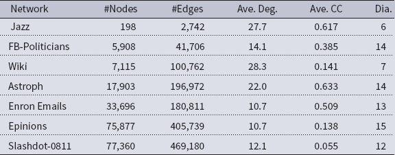
Networks: The seven networks of Table 4 are evaluated. We use only the giant components from the networks. Properties were generated with the the codes in Ahmed et al. (Reference Ahmed, Alo, Amelink, Baek, Chaudhary, Collins, Esterline, Fox, Fox, Hagberg, Kenyon, Kuhlman, Leskovec, Machi, Marathe, Meghanathan, Miyazaki, Qiu, Ravi, Rossi, Sosic and von Laszewski2020) and using the structural analysis libraries of NetworkX (Hagberg et al. Reference Hagberg, Schult and Swart2008) and SNAP (Leskovec & SosiČ Reference Leskovec and SosiČ2016).
Table 4. Networks used in experiments, and selected properties. All properties are for the giant component of each graph. The last three columns in the table give the average node degree, average clustering coefficient and diameter respectively
5.2 Simulation process
A simulation consists of a set of iterations. Each iteration consists of software execution of contagion propagation from an initial configuration. This configuration consists of a seed set A of 20 nodes, where seed nodes possess at least one contagion (i.e., the state of each seed node is from {1, 2, or 3}). Each of the seed nodes has a probability of 1/3 of being set to each of states 1, 2, and 3. The remainder of the nodes in the initial configuration possess no contagion and are thus in state 0.
The total number of seed nodes is 20 in all simulation iterations, and these nodes are chosen from the 20-core Footnote 1 of each graph. Selecting seed nodes from the 20-core, where nodes are more well connected with other high-degree nodes, makes blocking contagion spreading more difficult. There are two seeding methods. One method, which we refer to as “random 20-core,” selects uniformly at random 20 nodes from the 20-core. The second method selects a single node uniformly randomly and adds 19 of its distance-1 neighbors, not necessarily from the 20-core, so that these seed nodes induce a connected subgraph. We refer to this as the “Centola method” since it has been used in Centola (Reference Centola2009) and Centola & Macy (Reference Centola and Macy2007). Each of the 100 iterations of a simulation has a different seed set. The 100 seed sets (one for each iteration) are reused in all simulations for 1 graph so that the results for different blocking methods can be compared on a per-iteration basis. The great majority of results are presented for the Centola seeding method; the results for the random 20-core method are qualitatively similar. There are two exceptions: (i) in the timing studies of Section 5.3.6, we use software execution durations from both methods to increase the number of timing data points, and (ii) in Section 5.3.8, where we compare the blocking results for the two seeding methods.
An iteration starts at $t=0$
with the seed nodes as the only activated nodes. From these nodes, contagion propagates in discrete times
$t=0$
with the seed nodes as the only activated nodes. From these nodes, contagion propagates in discrete times $t \in [1~..~t_{\max}]$
as described in Section 2. All state transitions, x to y, are recorded for all
$t \in [1~..~t_{\max}]$
as described in Section 2. All state transitions, x to y, are recorded for all $v \in V$
. In this work, our simulations use uniform thresholds for all nodes and all state transitions for one simulation, so we abbreviate the thresholds below by setting
$v \in V$
. In this work, our simulations use uniform thresholds for all nodes and all state transitions for one simulation, so we abbreviate the thresholds below by setting $\theta = \theta(v, x, y)$
. We run 100 iterations per simulation, where the differences among the iterations is the composition of the seed node sets. Simulations are run with and without blocking nodes, as explained in the next subsection.
$\theta = \theta(v, x, y)$
. We run 100 iterations per simulation, where the differences among the iterations is the composition of the seed node sets. Simulations are run with and without blocking nodes, as explained in the next subsection.
Our experiments were performed on a Linux compute cluster. This cluster is composed of Dell PowerEdge C6420 2.666 GHz hardware nodes, with 384 GB RAM and 40 cores per node. Each core in a node is an Intel Xeon Gold 6148, 2.40 GHz with 1280 KiB L1 cache, 20 MiB L2 cache, and 27 MiB L3 cache. Our simulator is a serial code.
Summary of Analysis Process: The steps in our computational experiments are presented in Figure 5. From the left, inputs to simulations include a network from Table 4, threshold model and values, and initial conditions. Outputs are the states of all nodes at all discrete time steps between $t=0$
and
$t=0$
and $t_{\max}$
. These outputs, as well as the blocking method, and budget
$t_{\max}$
. These outputs, as well as the blocking method, and budget $\beta_i$
on blocking nodes for contagion
$\beta_i$
on blocking nodes for contagion $\mathbb{C}_i$
, are inputs to the blocking code. Outputs are the blocking nodes for each iteration of a simulation. The blocking nodes are added to the otherwise identical earlier simulation iteration, rerun at this point, to compute the efficacy of the blocking nodes. Unless otherwise stated, all results are averages over all 100 iterations of a simulation.
$\mathbb{C}_i$
, are inputs to the blocking code. Outputs are the blocking nodes for each iteration of a simulation. The blocking nodes are added to the otherwise identical earlier simulation iteration, rerun at this point, to compute the efficacy of the blocking nodes. Unless otherwise stated, all results are averages over all 100 iterations of a simulation.
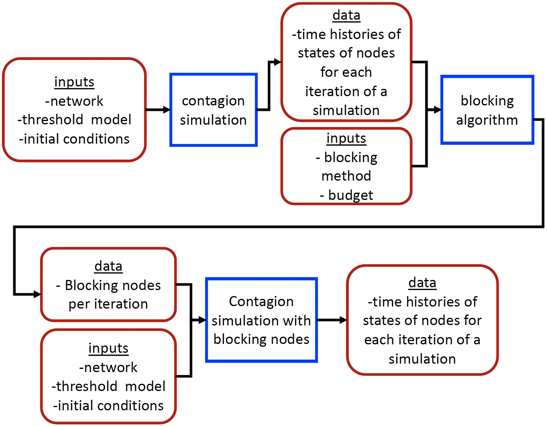
Figure 5. Steps in numerical experiments to identify and evaluate blocking nodes for inhibiting the spread of multiple contagions. Software modules are in blue boxes and data are in brown boxes.
5.3 Simulation and blocking results
5.3.1 Overview of experimental results
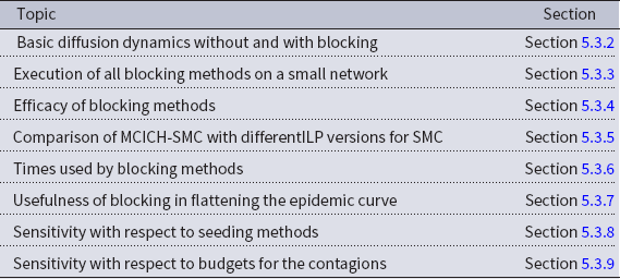
In the remainder of this section, we discuss results from the experiments conducted using the blocking methods discussed in Section 4. The different topics covered by our experiments are summarized in Table 5.
Table 5. Topics addressed in our experiments and the corresponding subsections
5.3.2 Basic diffusion dynamics without and with blocking
Figure 6 provides three types of results for the FB-Politicians network. The first two plots show temporal data on the spread or propagation of both contagions $\mathbb{C}_1$
and
$\mathbb{C}_1$
and $\mathbb{C}_2$
simultaneously without blocking. The third plot shows temporal effects of blocking on the propagation of both contagions. Figure 6(a) shows the number of newly activated infections at each time step. The curves rise as uniform threshold decreases from 4 to 3 to 2, since contagion propagates more readily for lesser thresholds. Figure 6(b) shows the corresponding plots of total or cumulative number of nodes activated for both contagions as a function of time. Roughly 50% to 70% of FB-Politicians nodes are activated by
$\mathbb{C}_2$
simultaneously without blocking. The third plot shows temporal effects of blocking on the propagation of both contagions. Figure 6(a) shows the number of newly activated infections at each time step. The curves rise as uniform threshold decreases from 4 to 3 to 2, since contagion propagates more readily for lesser thresholds. Figure 6(b) shows the corresponding plots of total or cumulative number of nodes activated for both contagions as a function of time. Roughly 50% to 70% of FB-Politicians nodes are activated by $t_{\max}=10$
, depending on
$t_{\max}=10$
, depending on $\theta$
. Figure 6(c) uses the
$\theta$
. Figure 6(c) uses the $\theta=3$
data from Figure 6(b) as a baseline and shows three additional curves corresponding to the blocking methods random, high degree, and MCICH-SMC. These data show that for a blocking budget
$\theta=3$
data from Figure 6(b) as a baseline and shows three additional curves corresponding to the blocking methods random, high degree, and MCICH-SMC. These data show that for a blocking budget $\beta_i=0.02$
fraction of nodes, the MCICH-SMC performs best (i.e., the curve is the lowest). For blocking contagions, “lesser” (or “lower”) is better. However, this budget is insufficient to completely halt the contagions. Note that in all three plots, and in those below, the total number of infections—from which the fractions on the y-axis are computed—is 2n, where
$\beta_i=0.02$
fraction of nodes, the MCICH-SMC performs best (i.e., the curve is the lowest). For blocking contagions, “lesser” (or “lower”) is better. However, this budget is insufficient to completely halt the contagions. Note that in all three plots, and in those below, the total number of infections—from which the fractions on the y-axis are computed—is 2n, where $n=|V|$
, because each node can acquire both contagions.
$n=|V|$
, because each node can acquire both contagions.

Figure 6. Simulation results for the FB-Politicians network, where results are averages over 100 iterations. Part (a) shows time histories of the average number of newly activated nodes at each time step for contagions $\mathbb{C}_1$
and
$\mathbb{C}_1$
and $\mathbb{C}_2$
, for three thresholds. Part (b) shows time histories of the average number of cumulative activated nodes at each time step for contagion
$\mathbb{C}_2$
, for three thresholds. Part (b) shows time histories of the average number of cumulative activated nodes at each time step for contagion $\mathbb{C}_1$
and
$\mathbb{C}_1$
and $\mathbb{C}_2$
, for the same thresholds. Part (c) provides data for
$\mathbb{C}_2$
, for the same thresholds. Part (c) provides data for $\theta=3$
, for no blocking, and for each of the three blocking methods mentioned in the legend, where the blocking node budget
$\theta=3$
, for no blocking, and for each of the three blocking methods mentioned in the legend, where the blocking node budget $\beta_i=0.02$
fraction of nodes. No method completely blocks the contagion (i.e., a greater budget is required for doing so), but MCICH-SMC performs best over the entire time history.
$\beta_i=0.02$
fraction of nodes. No method completely blocks the contagion (i.e., a greater budget is required for doing so), but MCICH-SMC performs best over the entire time history.
In the subsequent figures, we focus on the fraction of possible infections at fixed point conditions (i.e., the ending data points in the curves of Figure 6(c)) and often plot these points as a function of the blocking budget $\beta_i$
for different networks, thresholds, and initial simulation conditions.
$\beta_i$
for different networks, thresholds, and initial simulation conditions.
5.3.3 Application of all the blocking methods on a small network
Figure 7 shows the blocking performance of several methods on a small network, namely Jazz. In addition to no blocking results, blocking method results are shown for high degree, MCICH-SMC, MCICH-SMC-ILP, and optimal solution method, denoted by OPT-ILP. (Recall that OPT-ILP uses the ILP formulation discussed in Section 4.2). Because the network is small (it has only 198 nodes), all of the computations for all of the methods completed in all iterations. This is in contrast to results on larger networks where OPT-ILP did not finish for many iterations. As the blocking budget increases, all of the methods produce decreases in the fraction of possible infections, with optimal showing the best performance, as expected. The curves are the mean over all 100 iterations. The rates of these decreases can vary markedly among the methods. The two versions of our heuristic MCICH (namely, MCICH-SMC-Greedy and MCICH-SMC-ILP) have similar performance, and their performance is significantly better than that of the high-degree method. For the same budget, each blocking method performs better when the threshold is increased from 2 to 3. This is because it is more difficult to propagate a contagion as threshold increases.

Figure 7. Results for a small network (Jazz), for all blocking methods, showing the performance of the methods and the variability in results from the replicates of simulations. Parts (a) and (b) show the results for threshold values of 2 and 3 respectively. For each curve, the bands shows values within one standard deviation of the mean curve. The variability is caused by the different seed sets across iterations; see text. In the legend, the names MCICH-SMC, MCICH-ILP and Optimal refer to the variants MCICH-SMC, MCICH-SMC-ILP and OPT-ILP respectively.
The variability in results in Figure 7, as represented by standard deviation, can overlap across methods. For example, the variabilities for OPT-ILP, MCICH-SMC-Greedy, and MCICH-SMC-ILP are such that their scatter bands overlap. This is caused by the different seed sets and is not caused by randomness in the methods themselves. Specifically, for each blocking budget, there are 100 iterations, so averages are taken over all of these iterations that have different seed sets. Some seed sets are more onerous (i.e., more difficult to block) than others. We have compared results across methods on an iteration-by-iteration basis—across all of the networks—and found, for example, that the optimal method always does better than (or at least as good as) the MCICH-SMC-Greedy and MCICH-SMC-ILP methods.
5.3.4 Efficacy and comparisons of blocking methods across networks
Figures 8 and 9 depict the efficacy of the simple heuristics (random and high degree), OPT-ILP, and MCICH-SMC for six networks, for threshold values $\theta=2$
, 3, and 4. Each of the two figures presents results for three networks. The numbers of nodes in these networks varies from about 5,900 to 77,000 (see Table 4). Data for one network are in a row, and data for one threshold are in one column. The y-axis presents the cumulative fraction of possible infections; recall that the number of possible infections is twice the number of nodes since each node may be infected once by each contagion. The x-axis depicts the blocking budget in terms of the fraction of each network’s nodes. The cumulative fraction of possible infections corresponds to the points at
$\theta=2$
, 3, and 4. Each of the two figures presents results for three networks. The numbers of nodes in these networks varies from about 5,900 to 77,000 (see Table 4). Data for one network are in a row, and data for one threshold are in one column. The y-axis presents the cumulative fraction of possible infections; recall that the number of possible infections is twice the number of nodes since each node may be infected once by each contagion. The x-axis depicts the blocking budget in terms of the fraction of each network’s nodes. The cumulative fraction of possible infections corresponds to the points at $t_{\max}$
in curves such as those presented in Figure 6(c), for the respective blocking methods, thresholds, and networks. There is a “no blocking” curve, and five curves for blocking methods: one for each of the random blocking nodes heuristic, high-degree blocking nodes heuristic, MCICH-SMC-Greedy, MCICH-SMC-ILP, and OPT-ILP in each plot. Since lower curves represent more effective blocking, it is clear that the two MCICH-SMC methods perform far better, in the great majority of cases, compared to the random and high-degree blocking heuristics. The two variants of our heuristic MCICH, namely MCICH-SMC-Greedy and MCICH-SMC-ILP-High Time, have very similar performance across the six networks.
$t_{\max}$
in curves such as those presented in Figure 6(c), for the respective blocking methods, thresholds, and networks. There is a “no blocking” curve, and five curves for blocking methods: one for each of the random blocking nodes heuristic, high-degree blocking nodes heuristic, MCICH-SMC-Greedy, MCICH-SMC-ILP, and OPT-ILP in each plot. Since lower curves represent more effective blocking, it is clear that the two MCICH-SMC methods perform far better, in the great majority of cases, compared to the random and high-degree blocking heuristics. The two variants of our heuristic MCICH, namely MCICH-SMC-Greedy and MCICH-SMC-ILP-High Time, have very similar performance across the six networks.

Figure 8. Performance comparison of blocking methods for Astroph, FB-Politicians and Wiki for three threshold values, namely 2, 3 and 4. See main text for additional discussion regarding these plots. In the legend, the name Optimal refers to OPT-ILP.
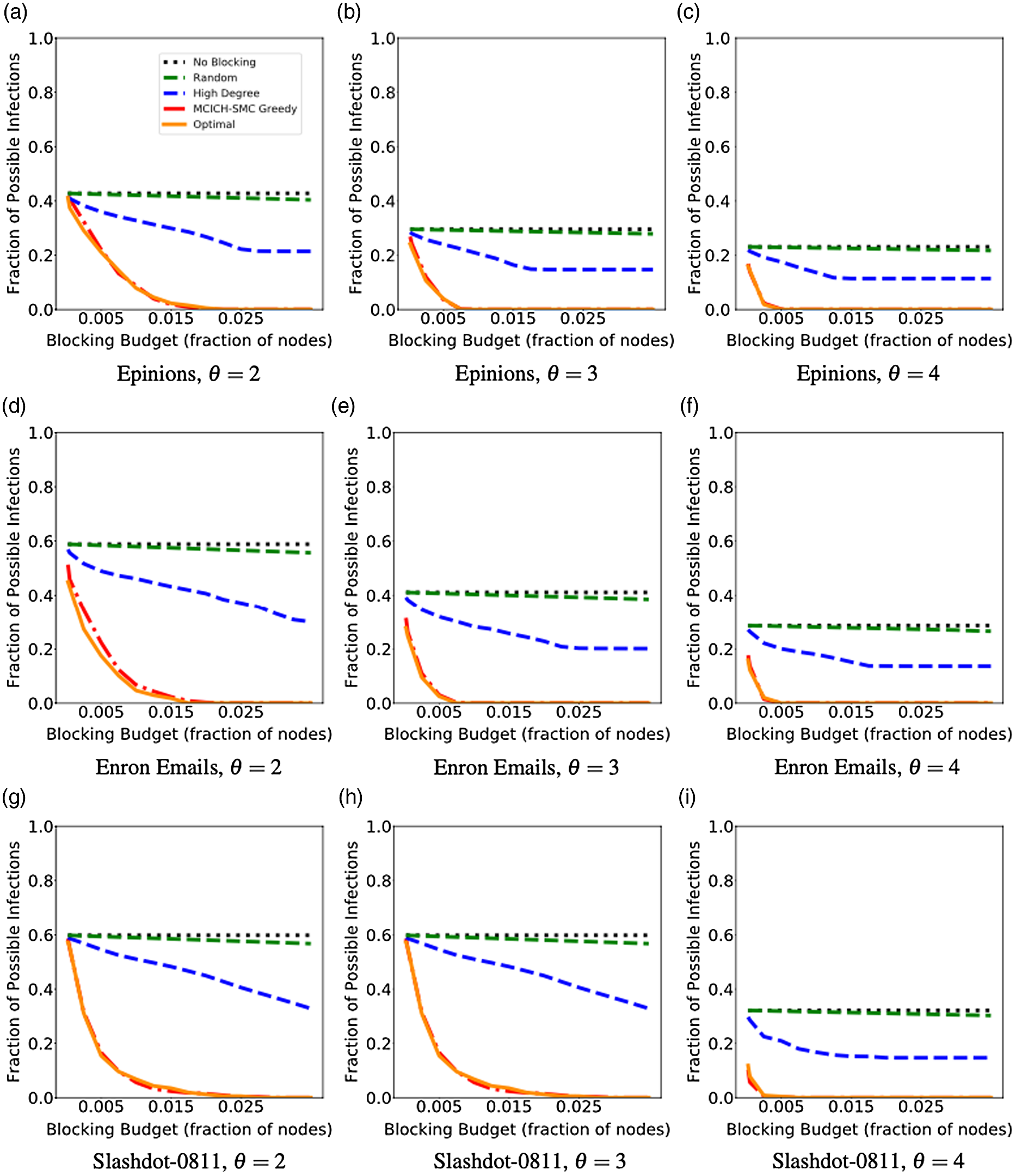
Figure 9. Performance comparison of blocking methods for three more networks, namely Epinions, Enron Emails and Slashdot-0811 for threshold values of 2, 3 and 4. See main text for additional discussion regarding these plots. In the legend, the name Optimal refers to OPT-ILP.
The reader would notice that our optimal ILP-based algorithm seems to have a worse performance than MCICH in some cases (e.g., Figures 8(i), 9(g)). This is not the case; this apparent discrepancy is due to the fact that the optimal method and MCICH-SMC-ILP method did not terminate in some of the iterations for large networks in a reasonable amountFootnote 2 of time. Since we computed averages using the values from the iterations in which the optimal algorithm and MCICH-SMC-ILP terminated, the figures give the impression of a discrepancy. Additional examples of this apparent discrepancy are presented in Section 5.3.5. Clearly, this behavior cannot occur in cases when the two ILP-based methods terminate in all iterations.
5.3.5 Comparison of several versions of MCICH-SMC that use ILP for SMC
Here, the time parameter selected for the ILP-based solution method (MCICH-SMC-ILP) and its effect on blocking efficacy is studied. This supplements the apparently anomalous blocking performance due to limited execution times, as noted in Section 5.3.4.
Figure 10 provides worst-case MCICH-SMC-ILP-based behaviors for Wiki, Epinions, and Slashdot-0811. “Worst case” in this context means abrupt changes in solution results for changing blocking budgets; for example, see the magenta curves, corresponding to the MCICH-SMC-ILP Moderate Times, in the plots of this figure.

Figure 10. Blocking results from all methods for some larger networks to show that some methods do not terminate in a reasonable amount of time. In the legend the name Optimal refers to OPT-ILP.
Recall that MCICH-SMC-ILP solves one instance of the SMC problem for each set $S_t$
of newly infected nodes at time t (found during the initial simulation which does not use any blocking). For networks of substantial size, which for our methods are networks of roughly 10,000 nodes, these computations are time-consuming. Execution duration may be controlled using a maximum time or integrality gap parameter in the Gurobi ILP solver (Gurobi Optimizer Reference Manual 2020) which halts the computations and uses the best feasible solution that the ILP solver has found until that time. To understand the effect of the time parameter, three time limits are applied to the method: 120 seconds, 28,800 seconds, and 521,700 seconds, which are labeled low, moderate, and high time, respectively (as mentioned in Section 4). As seen in Figure 10, the MCICH-SMC-ILP with low time (cyan curves) performs almost identically to MCICH-SMC-Greedy, although its execution duration is greater. MCICH-SMC-ILP, with moderate time, does not finish all iterations within our maximum allowable execution time, so averages in the plots of Figure 10 for this method (magenta curves) do not produce data that can be used for comparison among methods. The step-like nature of the moderate time curve (Part (c) of Figure 10) is likely due to the ILP becoming stuck in local optima which it cannot leave in its allotted time. MCICH-SMC-ILP with high time did not finish even one iteration for all blocking budget values in the plots depicted in the figure, so it is not plotted.
$S_t$
of newly infected nodes at time t (found during the initial simulation which does not use any blocking). For networks of substantial size, which for our methods are networks of roughly 10,000 nodes, these computations are time-consuming. Execution duration may be controlled using a maximum time or integrality gap parameter in the Gurobi ILP solver (Gurobi Optimizer Reference Manual 2020) which halts the computations and uses the best feasible solution that the ILP solver has found until that time. To understand the effect of the time parameter, three time limits are applied to the method: 120 seconds, 28,800 seconds, and 521,700 seconds, which are labeled low, moderate, and high time, respectively (as mentioned in Section 4). As seen in Figure 10, the MCICH-SMC-ILP with low time (cyan curves) performs almost identically to MCICH-SMC-Greedy, although its execution duration is greater. MCICH-SMC-ILP, with moderate time, does not finish all iterations within our maximum allowable execution time, so averages in the plots of Figure 10 for this method (magenta curves) do not produce data that can be used for comparison among methods. The step-like nature of the moderate time curve (Part (c) of Figure 10) is likely due to the ILP becoming stuck in local optima which it cannot leave in its allotted time. MCICH-SMC-ILP with high time did not finish even one iteration for all blocking budget values in the plots depicted in the figure, so it is not plotted.
This brings up practical issues when using MCICH-SMC-ILP. First, perhaps counterintuitively, lesser values of the integrality gap parameter may give better results, even though the resulting computational time is less. Second, one must perform scoping studies to determine the ranges of parameters that work best. Third, a more computationally efficient method, like MCICH-SMC, can provide the context for comparing and evaluating different ILP parameter settings. This last issue—computational execution time—is addressed in the next subsection.
5.3.6 Comparison of execution times of blocking methods
In this subsection, we compare the execution times of MCICH-SMC and the ILP-based optimal algorithm. Since the blocking performance of MCICH-SMC with greedy method for SMC is close to that of MCICH-SMC-ILP, we compare the execution times of MCICH-SMC-Greedy and the optimal method for six of our networks. The running times are shown as bar charts in Figure 11, where the networks are shown in increasing order of the number of nodes. The bar charts represent the average execution times across all iterations for threshold values of 2 and 4, respectively.

Figure 11. Comparison of execution times of MCICH-SMC and the ILP approach for six networks. The networks are listed in increasing order of the number of nodes. Figure (a) shows the results where each node has a threshold of 2 for each contagion while Figure (b) shows the results where each node has a threshold of 4 for each contagion. The red and orange bars represent respectively the times used by MCICH-SMC with the greedy approach for SMC and the optimal solution using the ILP. The comparison of execution times between the two methods is conservative because the optimal ILP solution computations did not finish for 53.1% of iterations. The thin vertical line at the top of each bar denotes one standard deviation.
It can be seen that in all cases, the execution time of MCICH-SMC-Greedy is several orders of magnitude less than that of the optimal method. It should be noted that while MCICH-SMC-Greedy completed in all iterations for all networks within the allotted execution times, the optimal algorithm did not complete for some iterations of a simulation within the 145-hour time limit for these computations. We computed the average execution time for the optimal method using the times for the iterations where it completed within the maximum time limit. So, the actual average execution time is larger for the optimal solution method than what is shown in the bar charts of Figure 11. Thus, one should not conclude that the difference between the optimal method and MCICH-SMC-Greedy decreases as network size increases. Further, the execution times for the Wiki network are larger than some of the larger networks, since the average degree of Wiki is the largest among the networks considered in our work (see Table 4).
5.3.7 Usefulness of blocking in flattening the epidemic curve
In this subsection, we compare the benefits of two variants of MCICH-SMC-Greedy. One of these variants (referred to as “Before-Peak”) chooses the blocking nodes for each contagion, and for each simulation iteration, at a time step before the number of new infections for that contagion reaches a peak in the simulation where no blocking nodes are used. The other variant (referred to as “Unconstrained”) has no such restriction; it may choose the blocking nodes for each contagion at any time step. The comparison between these two variants was done for two networks (Wiki and FB-Politicians) for two different budgets on the number of blocking nodes. We used the threshold values of 2 and 3, respectively, for Wiki and FB-Politicians networks.
The results are shown in Figure 12. The curves in these plots show the total number of new infections across both contagions in each time step. In all cases, it is observed that the two variants of MCICH-SMC-Greedy do not delay the time of occurrence of the peak value; however, they reduce the number of peak infections compared to no blocking. In particular, the Before-Peak variant performs better than the Unconstrained variant in all cases by decreasing the peak number of new infections significantly compared to the no blocking case. This contrasts with findings that the Before-Peak and Unconstrained variants of MCICH-SMC-Greedy do not differ significantly in the cumulative number of infections.

Figure 12. The effect of blocking by MCICH-SMC for the FB-Politicians and Wiki networks when blocking for each contagion is done in two ways: (i) blocking is unconstrained (i.e., it may be done at any time step) and (ii) blocking is done before the number of new infections (without any blocking) reaches a peak. The latter approach lowers the peak number of new infections better than the former method. The black curves show the number of new infections without any blocking.
5.3.8 Sensitivity with respect to seeding methods
Recall from Section 5.2 that two seeding methods were used to choose the set of initially infected nodes. Here, we study the sensitivity of MCICH-SMC-Greedy with respect to these methods, namely the method due to Centola (Reference Centola2009) and the one that chooses seed nodes randomly, both of which are based on the K-core of a network. The seed nodes were chosen from the 20-core of the network so as to encourage diffusion. In our experiments, we chose the FB-Politicians network and two threshold values, namely 2 and 3. The results are shown in Figure 13.

Figure 13. Sensitivity of seeding methods on the fraction of infections for FB-Politicians for $\theta=2$
and 3. Here, the K-core seeding methods used
$\theta=2$
and 3. Here, the K-core seeding methods used $K=20$
.
$K=20$
.
We first discuss the case where the threshold is 2. In this case, for a small budget value (namely, 0.5% of the nodes), the diffusion due to random seeding method is harder to block (i.e., causes a larger number of new infections) compared to that due to Centola’s seeding method; however, as the budget is increased, the diffusion due to Centola’s method becomes harder to block.
We hypothesize that the random 20-core method is more difficult to block for threshold 2, when there are few blocking nodes, because nodes in the random seed set are more dispersed (i.e., seed nodes may not be connected to other seed nodes) and are likely to have many neighbors with at least two connections to the seed set (the no blocking outbreak sizes in Figure 8(d) support this idea). However, as the blocking budget increases, it is harder to disrupt contagion that emanates from Centola seeding, where seed nodes are more concentrated in one region of a graph (i.e., it is more difficult for blocking nodes to “surround” the Centola seed nodes). For this same reason, it is more difficult to completely stymie both contagions (i.e., drive contagion spreading to zero) when seeded with Centola method.
Addressing the threshold three results, the reasons for the Centola seeding method being harder to block are as follows. First, as threshold increases, it is generally more difficult to initiate contagion spreading from seed nodes (Kuhlman et al. Reference Kuhlman, Kumar, Marathe, Ravi and Rosenkrantz2015). This is particularly the case in this study for FB-Politicians, as seen by the decreases in the “no blocking” black curves, from 0.80 to 0.25 in Figure 8(d) through (f) as threshold increases from 2 to 4. Second and consequently, it is more important, as threshold increases, to concentrate seed nodes in one region of a graph so that uninfected nodes at distance-1 from seed nodes can meet their thresholds and thus transition state. This is because social networks have considerable clustering (as measured by clustering coefficients in Table 4), so uninfected nodes with one infected neighbor are more likely to also be connected to other infected neighbors, and thus are better able to meet their thresholds. The Centola method concentrates seed nodes better than the random seeding method, making this method more difficult to block.
5.3.9 Sensitivity with respect to allocation of budget between the two contagions
In this subsection, we study how blocking methods allocate node budgets for each contagion $\mathbb{C}_1$
and
$\mathbb{C}_1$
and $\mathbb{C}_2$
. Figure 14 provides the results. In Figure 14(a), the now-familiar blocking results for MCICH-SMC-Greedy and OPT-ILP are provided. Figure 14(b) shows how the two methods allocate budget between the two contagions, to achieve these blocking results.
$\mathbb{C}_2$
. Figure 14 provides the results. In Figure 14(a), the now-familiar blocking results for MCICH-SMC-Greedy and OPT-ILP are provided. Figure 14(b) shows how the two methods allocate budget between the two contagions, to achieve these blocking results.
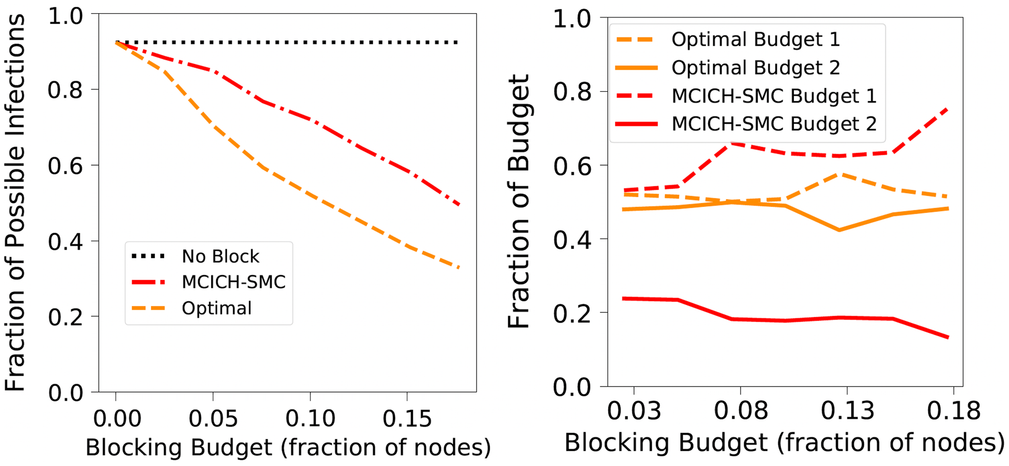
Figure 14. Figure showing sensitivity with respect to budget allocation. That is, how the blocking methods allocate the total budget of blocking nodes between the two contagions. Jazz network with a threshold value of 2 was used in these experiments. Part (a) shows the efficacy of the blocking nodes. Part (b) shows the fraction of budget allocated to the two contagions for each of the two methods.
Figure 14(b) shows the difference in how MCICH-SMC-Greedy and OPT-ILP split their budget across contagions $\mathbb{C}_1$
and
$\mathbb{C}_1$
and $\mathbb{C}_2$
. The difference in their budget splits helps explain the difference between their execution performance presented in Section 5.3.6. MCICH-SMC-Greedy chooses all blocking nodes for each contagion from one set of nodes which were all infected during the same time step (during the simulation without blocking nodes). (The times at which each of the two contagions is blocked may be different.) For that reason, MCICH-SMC-Greedy does not always exhaust its budget, as is evident from Figure 14; the Y-axis values for the two red curves do not sum to 1. OPT-ILP may choose nodes that are infected at any of the time steps (and across time steps) and considers global effects that MCICH-SMC-Greedy does not. Both of these factors contribute to the more even split seen in the budget allocation for OPT-ILP. Note that mirroring the 50%–50% budget allocation split given by OPT-ILP may not necessarily improve the performance of MCICH-SMC-Greedy because MCICH-SMC-Greedy cannot distribute its blocking budget across nodes infected at different time steps.
$\mathbb{C}_2$
. The difference in their budget splits helps explain the difference between their execution performance presented in Section 5.3.6. MCICH-SMC-Greedy chooses all blocking nodes for each contagion from one set of nodes which were all infected during the same time step (during the simulation without blocking nodes). (The times at which each of the two contagions is blocked may be different.) For that reason, MCICH-SMC-Greedy does not always exhaust its budget, as is evident from Figure 14; the Y-axis values for the two red curves do not sum to 1. OPT-ILP may choose nodes that are infected at any of the time steps (and across time steps) and considers global effects that MCICH-SMC-Greedy does not. Both of these factors contribute to the more even split seen in the budget allocation for OPT-ILP. Note that mirroring the 50%–50% budget allocation split given by OPT-ILP may not necessarily improve the performance of MCICH-SMC-Greedy because MCICH-SMC-Greedy cannot distribute its blocking budget across nodes infected at different time steps.
The reader will notice that for MCICH-SMC-Greedy, the budget allocations for contagions $\mathbb{C}_1$
and
$\mathbb{C}_1$
and $\mathbb{C}_2$
diverge as the budget increases. The reason for this is the following. After performing blocking for a given contagion, the leftover budget is allocated to the other contagion.
$\mathbb{C}_2$
diverge as the budget increases. The reason for this is the following. After performing blocking for a given contagion, the leftover budget is allocated to the other contagion.
Thus, the unbalanced budget allocation between the two contagions in Figure 14 is caused by MCICH-SMC-Greedy being unable to use the increased budget to block $\mathbb{C}_2$
, but MCICH-SMC-Greedy is still finding more opportunities to block
$\mathbb{C}_2$
, but MCICH-SMC-Greedy is still finding more opportunities to block $\mathbb{C}_1$
. These opportunities could mean MCICH-SMC-Greedy found a larger set to choose blocking nodes from or that MCICH-SMC-Greedy is able to block more nodes from a previously selected set.
$\mathbb{C}_1$
. These opportunities could mean MCICH-SMC-Greedy found a larger set to choose blocking nodes from or that MCICH-SMC-Greedy is able to block more nodes from a previously selected set.
It is an important result of this study that the simplifying constraint that all blocking nodes for one contagion must be applied at one time step for MCICH-SMC-Greedy still leads to very good blocking efficacy. Thus, very good blocking performance is achieved with the best execution performance.
6. Summary, limitations, and future work
We considered the problem of minimizing the number of new infections in a network through vaccination when two independent contagions are propagating through a network and there is a budget constraint on the number of vaccinations. Since the problem is computationally intractable, we developed an efficient heuristic algorithm and demonstrated its performance through experiments.
There are several directions for future work. Some of these directions arise due to limitations of our study. For example, it is of interest to evaluate the MCICH-SMC heuristic under several other scenarios; examples include graphs with nonuniform threshold values for nodes, other ways of selecting seed sets, and skewed distributions of seed nodes between the two contagions. Our computational intractability result for the VS-MTNNI problem assumes that the budget constraint cannot be violated. It is of interest to investigate whether efficient approximation algorithms can be developed assuming that the vaccination budget can be violated by a small factor. Further, one may consider restricted classes of graphs (e.g., graphs with bounded node degrees) and investigate whether efficient algorithms or approximations can be developed for those classes. In our model, the two contagions are assumed to be independent. It is of interest to consider a model where the contagions interact, that is, a node that is infected one contagion may make it easier or harder for the node to be infected by the other contagion. Developing suitable problem formulations and algorithms for interacting contagions is an interesting research direction. Finally, our work considers the deterministic threshold model. Many models for disease propagation are stochastic in nature (see e.g., Marathe & Vullikanti Reference Marathe and Vullikanti2013; Hethcote Reference Hethcote2000). Developing appropriate techniques for blocking multiple contagions under various stochastic propagation models is a challenging research direction.
Acknowledgements
This work is partially supported by Virginia Department of Health (VDH) Grant PV-BII VDH COVID-19 Modeling Program VDH-21-501-0135, University of Virginia Strategic Investment Fund award number SIF160 and NSF Grants ACI-1443054 (DIBBS), IIS-1633028 (BIG DATA), CMMI-1745207 (EAGER), OAC-1916805 (CINES), CMMI-1916670 (CRISP 2.0), CCF-1918656 (Expeditions), and IIS-1908530.
Competing interests
None.
A preliminary version of this paper appeared as Carscadden, H. L., Kuhlman, C. J., Marathe, M. V., Ravi, S. S., & Rosenkrantz, D. J. (2020). Blocking the propagation of two simultaneous contagions over networks. In R. M. Benito, C. Cherifi, H. Cherifi, E. Moro, L. M. Rocha, & M. Sales-Pardo (Eds.), Proceedings of 9th international conference on complex networks and applications (complex networks) (pp. 455–468), Cham, Switzerland. Springer. https://doi.org/10.1007/978-3-030-65347-7_38


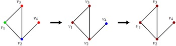


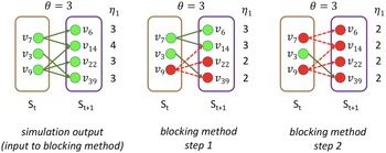


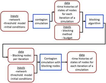

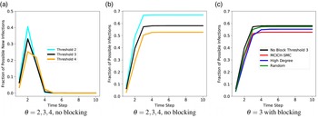


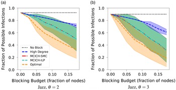
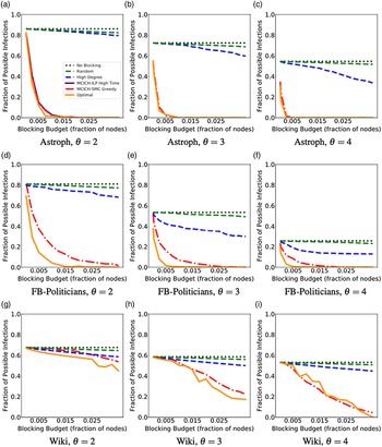
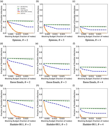
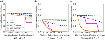
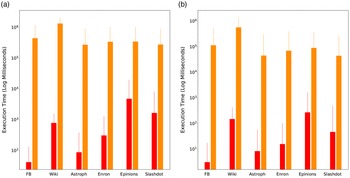
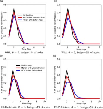
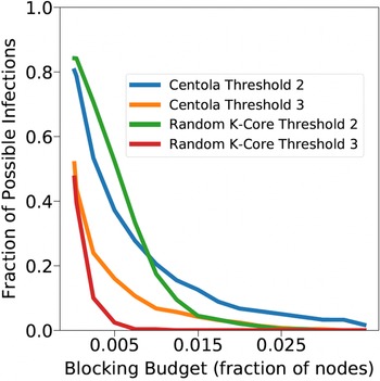


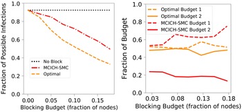

 Open access