


1. Introduction
Debris cover is a pertinent feature of Himalayan glaciers. About 10% of the total Himalayan glacierized area and ~40% of ablation areas are debris-covered with varying debris thickness ranging from a few centimeters to tens of centimeters (Bolch and others, Reference Bolch2012; Sharma and others, Reference Sharma2016; Miles and others, Reference Miles, Willis, Arnold, Steiner and Pellicciotti2017). There have been ample reports of continuous debris increase on the Himalayan glaciers (Bhambri and others, Reference Bhambri, Bolch, Chaujar and Kulshreshta2011; Ali and others, Reference Ali, Shukla and Romshoo2017; Patel and others, Reference Patel, Sharma, Fathima and Thamban2018; Garg and others, Reference Garg, Shukla and Jasrotia2019). Debris cover generally appears below the equilibrium line and can play an active role in modifying the ablation processes and overall morphology of the ablation tongues. Debris thickness pattern on debris-covered glacier tends to transition from convex- to concave-up-down glacier (Anderson and Anderson, Reference Anderson and Anderson2018) which may lead to differential downwasting and may cause slope inversion (Benn and others, Reference Benn2012). The changing ablation patterns and morphology can influence the glaciers' surface ice velocity (SIV). Previous studies clearly report progressive slow-down and stagnation of debris-covered glaciers in the Himalaya (Quincey and others, Reference Quincey, Luckman and Benn2009; Scherler and others, Reference Scherler, Bookhagen and Strecker2011; Bhattacharya and others, Reference Bhattacharya2016; Bhushan and others, Reference Bhushan, Syed, Kulkarni, Gantayat and Agarwal2017; Garg and others, Reference Garg, Shukla, Tiwari and Jasrotia2017). Stagnation has been defined as a very slow movement of the glacier. Obviously, there will be some movement in the ice for it to be considered a part of the glacier instead of ‘dead ice’. However, previous studies have adopted different thresholds of velocity to distinguish the stagnant portion of the glaciers. Scherler and others (Reference Scherler, Bookhagen and Strecker2011) termed a glacier portion stagnant if the velocity is <2.5 m a−1. Quincey and others (Reference Quincey, Luckman and Benn2009) did not specify a threshold, but designated lower debris-covered glacier tongues to be stagnant if these are moving very slowly (possibly <5 m a−1 as Fig. 3 in Quincey and other (Reference Quincey, Luckman and Benn2009) depicts). Shukla and Garg (Reference Shukla and Garg2019) defined SIV <10 m a−1 as a ‘very slow movement’. In the present study, we term a glacier part as stagnation if the SIV is <5 m a−1. Glacier stagnation can lead to a stable glacier terminus but such glaciers are susceptible to evolve new mass loss mechanism such as formation and development of ice cliffs. Ice cliffs, in turn, can account for ~7–40% of total wastage of a debris-covered portion (Immerzeel and others, Reference Immerzeel2014; Thompson and others, Reference Thompson, Benn, Mertes and Luckman2016; Steiner and others, Reference Steiner, Buri, Miles, Ragettli and Pellicciotti2019). Thus, it is important to identify the stagnant conditions of glaciers, the various processes leading to glacier stagnation and the consequences of stagnation.
Glacier response to climate changes is manifested through changes in glacier length, area, debris cover, SIV, surface elevation, snowline altitude (SLA) and formation/development of associated glacial lakes. Given the harsh environmental conditions of glaciated regions, the study of glacier parameters on the field is challenging and costly. This makes remote sensing perhaps the only viable alternative to study the glacial characteristics periodically (Paul and others, Reference Paul2013; Shukla and Qadir, Reference Shukla and Qadir2016). However, serious concern here is that most of the efforts in the Himalaya pertaining to remote sensing have been made toward assessing the dimensional changes (i.e. length and area) only (Vincent and others, Reference Vincent2013; Garg and others, Reference Garg, Shukla and Jasrotia2019). Dimensional variations are the simplest way of monitoring mountain glacier changes and have been used to infer climatic signals on both regional and global scales (Hoelzle and others, Reference Hoelzle, Haeberli, Dischl and Peschke2003; Leclercq and Oerlemans, Reference Leclercq and Oerlemans2012). However, it is necessary to note that these changes provide indirect, delayed and filtered responses of glaciers and are not a comprehensive assessment of the total glacier condition or health (Armstrong, Reference Armstrong2010; Zemp and others, Reference Zemp2015). Moreover, several recent studies have indicated that glaciers with apparently stable fronts may also lose significant mass through downwasting (Bolch and others, Reference Bolch, Pieczonka and Benn2011; Kargel and others, Reference Kargel, Cogley, Leonard, Haritashya and Byers2011; Immerzeel and others, Reference Immerzeel2014). Therefore, a multiparametric study is required in order to understand the comprehensive glacier response to climate change.
In the present study, the Pensilungpa glacier in the Suru river sub-basin has been selected for a detailed investigation. The study area falls in the monsoon-arid zone making it important for climate change-related studies (Pandey and others, Reference Pandey, Ghosh, Nathawat and Tiwari2011; Shukla and Qadir, Reference Shukla and Qadir2016). Considering the above-described aspects, the main goals of this paper are to (a) present a comprehensive picture of status and behavior of the Pensilungpa glacier by monitoring multiple glacier parameters namely length, area, SLA, SIV and surface elevation changes (SEC), (b) understand the influence of changing glacier parameters on the stagnation/ablation process and (c) evaluate the stagnant conditions of the glacier and its implications.
2. Study area and datasets
The Pensilungpa glacier (terminus coordinates: 33.845°N, 76.375°E) is a medium-sized (length: 8.51 km; area: 14.67 ± 0.29 km2 in 2016) valley-type glacier located in the Kargil district of Jammu and Kashmir (Fig. 1). It is situated near the Pensi-La pass, which is often referred to as the ‘Gateway to Zanskar’ (Kamp and others, Reference Kamp, Byrne and Bolch2011). The glacier surface is highly undulating and crevassed (Fig. 2). As per recent estimates (2016) of the present study, ~17.35% of total area of this glacier is covered with debris comprising fine-grained sand to large boulders (Fig. 2). The glacier flows north-east from an elevation of ~6000 m above sea level (a.s.l.) and terminates at 4668 m a.s.l. giving rise to the Suru River, which is an important tributary of the River Jhelum. The SLA of glacier is at 5160 m a.s.l. (2016) which divides glacier into accumulation zone (ACZ) and ablation zone (ABZ). The ABZ has been further divided into lower ablation zone (LAZ) and upper ablation zone (UAZ) considering the distinctive dynamics and geomorphological features of these zones as deduced in an integrative manner from the field and remote-sensing data (Fig. 1). The LAZ is characterized by a debris mantle of heterogeneous thickness but following the thinning upwards trend and very low SIVs (<5 m a−1). It has uneven and quite rugged topography probably owing to the unequal amount of surficial melting. Ice cliffs with varying aspects and trends, glacier tables, deep supraglacial channels and ephemeral meltwater accumulations/ponds are common occurrences in LAZ. While UAZ has relatively much smoother surface with very sparse debris cover, higher SIVs and a narrow and shallow network of supraglacial channels. The drop down in SIV at ~2 km from the snout (discussed in Section 4.2) is a clear indication of the transition from LAZ to UAZ; however, according to the field observations, the boundary between these two zones is fuzzy and not sharp. This is because surface feature characteristics of the LAZ continue for ~150–200 m beyond the maximum debris cover extent. Thus, the boundary between LAZ and UAZ roughly follows the debris cover extent and has an average elevation of ~4905 m a.s.l. (Fig. 1).
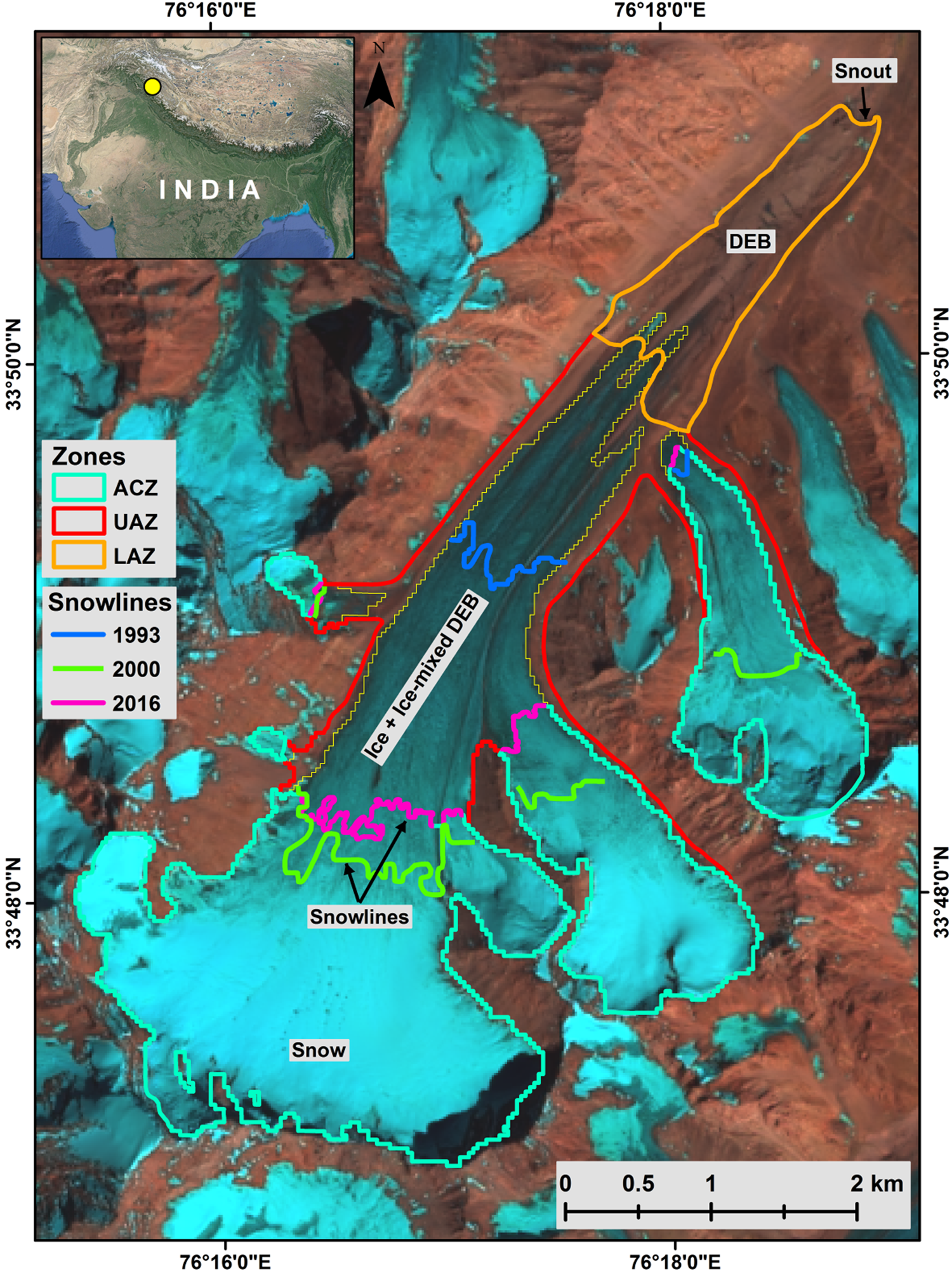
Fig. 1. Location of the study area. The glacier and debris cover (DEB) outlines overlain on map are of the year 2016. The background is a Landsat OLI image of 8 October 2016. Lower ablation zone (LAZ), upper ablation zone (UAZ) and accumulation zone (UAZ) and snowlines are also shown on the map.
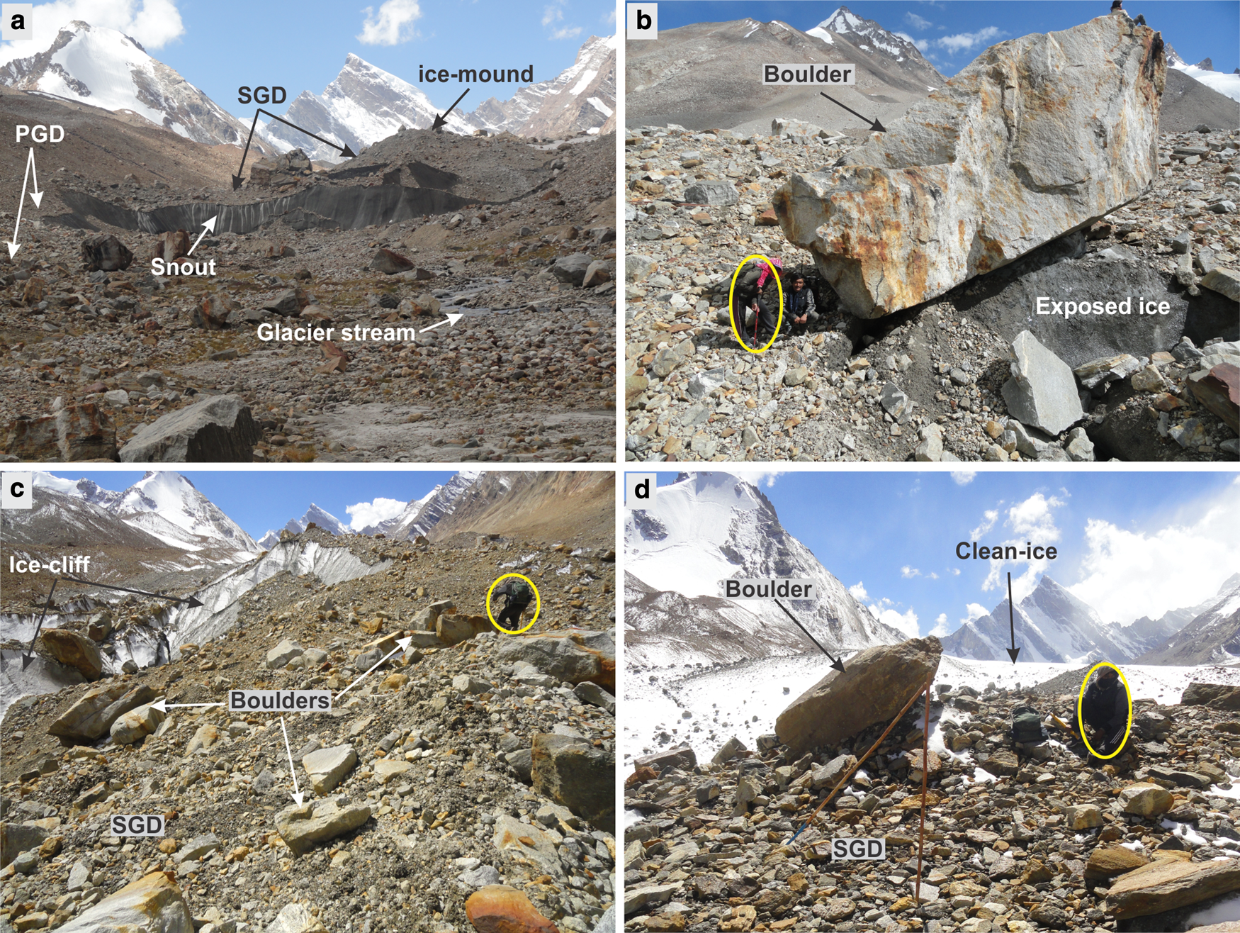
Fig. 2. Debris cover characteristics over the Pensilungpa glacier. Notice a large variation in the size of debris mantle ranging from a few millimeter to big boulders of several meters. Yellow ellipsoids marked on the photographs show human scale.
The prime reason for selection of this particular glacier for our study includes its accessibility (~150 km by road from Kargil town), medium size, well-defined ACZ and ABZ, and locality in the climatically crucial rain-shadow (semi-desert) zone (Archer and Fowler, Reference Archer and Fowler2004). The region alternatively receives snowfall during winter and rainfall during summer from westerlies and Indian summer monsoon (ISM), respectively. The average annual precipitation, recorded at the Leh meteorological station of this region, amounts only to ~250 mm (Shukla and Qadir, Reference Shukla and Qadir2016). Due to alternate influence of westerlies and ISM, the region experiences an annual temperature range from a winter minimum of 1.3 to −7.8°C to a summer maximum of 8.0–18.2°C. Shukla and others (Reference Shukla, Garg, Mehta, Kumar and Shukla2020) reported that the mean annual temperature in study region increased by 0.8°C over the period 1901–2017. The mean annual minimum temperature registered higher increase (1.3°C) than the mean annual maximum temperature (0.3°C) along with a simultaneous increase in the precipitation (~20%) during this period. Moreover, a conspicuous temperature rise after 1996 occurred in the region (Shukla and others, Reference Shukla, Garg, Mehta, Kumar and Shukla2020).
Gridded temperature and precipitation data from the Climate Research Unit (CRU) Time Series 4.01 (TS 4.01) having spatial extent of 0.5° × 0.5° latitudinal and longitudinal grids, covering the study region, have also been analyzed here for 1901–2016 period. The climate data show an annual average precipitation and temperature of 441 mm and 0.6°C, respectively, over the 115 years. Precipitation is observed in almost all the months with maxima in the months of July and August, followed by January and February. Also, July is the warmest while January is the coldest month in the region (Fig. 3). It is notable that the long-term temperature for November–April months remains well below 0°C (Fig. 3). Therefore, it can be inferred that these months likely receive solid precipitation. Conversely, temperature for the May–October months remains above 0°C (Fig. 3) indicating a likelihood of receiving liquid precipitation.
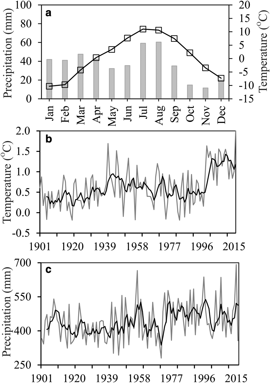
Fig. 3. Temperature and precipitation data for the study region acquired from CRU TS 4.01 dataset for the period of 1901–2016. Notice a continuous increase in temperature and almost no change in the precipitation, particularly in the recent decades. The step change in temperature after 1996 is particularly noticeable and corresponds well with previous studies (Bhutiyani and others, Reference Bhutiyani, Kale and Pawar2010; Harris and others, Reference Harris, Jones, Osborn and Lister2014; Shukla and others, Reference Shukla, Garg, Mehta, Kumar and Shukla2020). Solid black lines show 5-year moving average plots.
The study aims at evaluating glacier parameters for 1990, 2000 and 2015 time periods by utilizing remote-sensing data from various satellites and sensors. However, in case of unavailability of suitable (i.e. snow and cloud free) images, we had to use the next suitable images having 3–4 years gap from the target years. For estimation of glacier area, length, debris cover, snowlines and SIV, Landsat data from thematic mapper (TM; 1990 ± 4 years), Enhanced Thematic Mapper Plus (ETM +; 2000 ± 4 years) and Operational Land Imager (OLI; 2015 ± 4 years) have been utilized. All the Landsat images were acquired from the Earth Explorer website (https://earthexplorer.usgs.gov/). The SEC was quantified by subtracting Shuttle Radar Topographic Mission (SRTM) Digital Elevation Model (DEM) version-3 (v3) of 2000 from Advanced Spaceborne Thermal Emission and Reflection Radiometer (ASTER) DEM of 2017. The ASTER DEM was downloaded from the Earth Data website (https://search.earthdata.nasa.gov/). The SRTM DEM has been used here as the reference DEM and acquired from https://earthexplorer.usgs.gov/ which possesses a vertical accuracy of ±10 m (Rodriguez and others, Reference Rodriguez, Morris and Belz2006). The AST14 DMO product was used here as a secondary DEM and was procured from the https://search.earthdata.nasa.gov/. Table 1 lists the complete details of remote-sensing data used in this study. Further, considering the dynamic nature of SLA, we have carried out its time series mapping between 1993 and 2016 using diverse remote-sensing data (Supplementary Table S1).
Table 1. List of satellite data used in this study
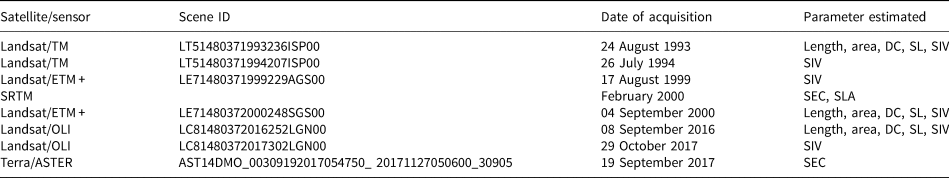
DC, debris cover; SL, snowline; SLA, snowline altitude; SIV, surface ice velocity; SEC, surface elevation change.
Field observations are required to closely understand the glacier characteristics and to address inherent uncertainties involved in mapping the glacier parameters from remotely sensed data. Field work campaigns to the Pensilungpa glacier were undertaken during the months of August–September in 2016, 2017 and 2018. Several glacier features were observed and photographed to understand the glaciers' current state (Figs 2, 4). Also, stakes were installed on the ABZ of the glacier in 2016 and 2017 and tracked using a Leica Geosystem Differential Global Positioning System (DGPS), which provides horizontal and vertical accuracies of ±10 and ±5 cm, respectively, in a mountainous terrain. A total number of ten ablation stakes were installed in the LAZ (4668–4905 m a.s.l.) of the glacier in 2016 which were measured in 2017 to calculate the annual point melting. In 2017, nine stakes could be measured as one stake was lost. Further, in addition to nine previously installed stakes, eight more stakes were installed in 2017 to cover the entire debris-covered portion of the glacier including some parts of UAZ. However, in 2018, only 11 stakes could be recovered.
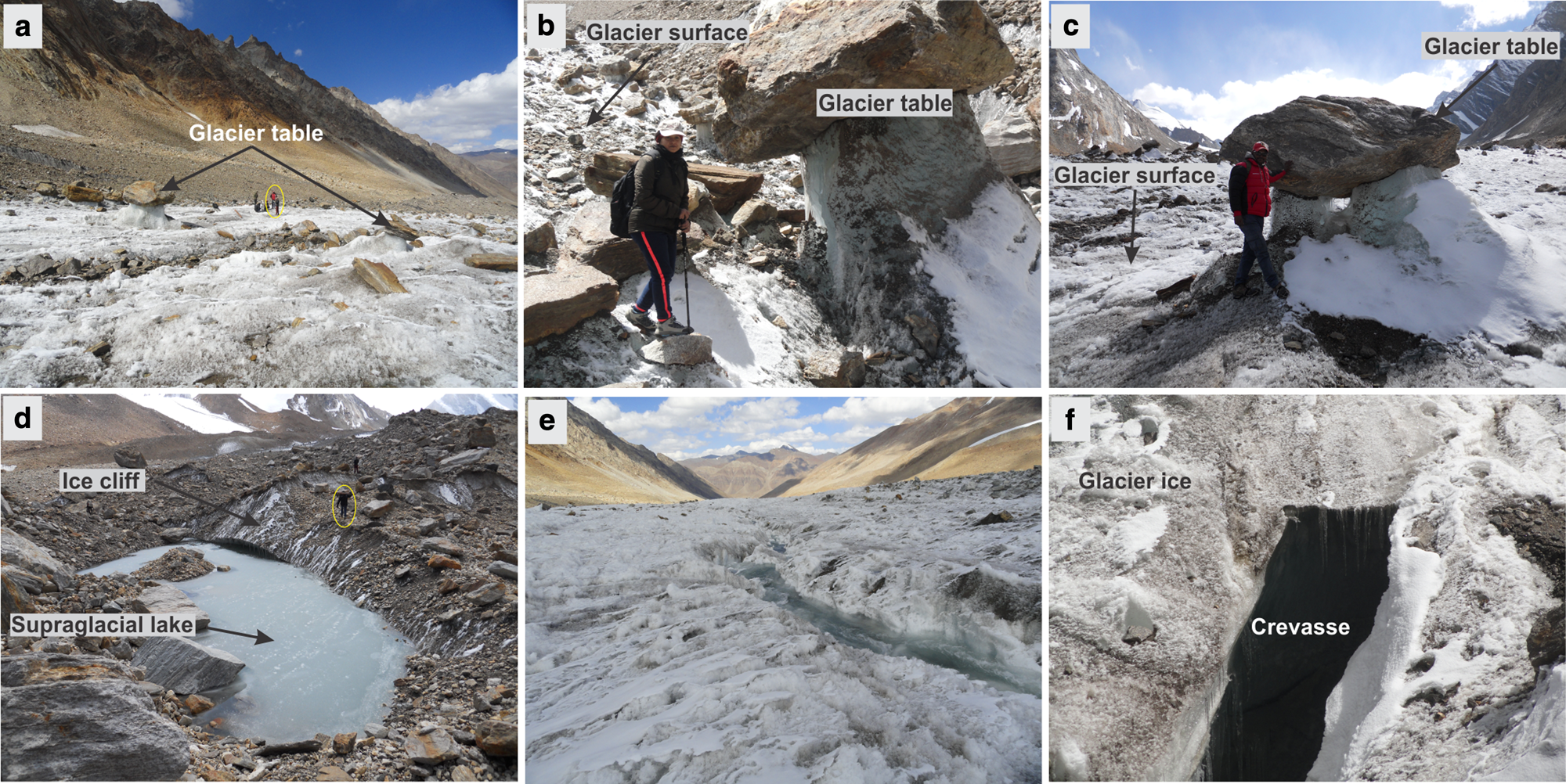
Fig. 4. Various glacial features such as (a–c) glacier tables, (d) glacial pond and associated ice cliffs, (e) supraglacial channel and (f) deep crevasse, observed during the field visit on the Pensilungpa glacier during the months of August–September in 2016 and 2017. The human scale is marked on the photographs (panels a and d) as yellow ellipsoids. Glacier tables with significant height (up to 2–2.5 m) clearly indicate differential melting and pronounced downwasting on the glacier.
3. Methodology
3.1. Glacier parameter extraction
Glacier boundaries (i.e. glacier area) were mapped in a two-step process. In the first step, we created band ratios using Red and Shortwave Infrared Bands (Red/SWIR) and applied a scene-specific threshold (ranging from 1.6 for OLI to 1.9 for TM) to automatically identify the clean-ice parts. The raster files thus generated were smoothened using a median filter (3 × 3) and converted to vector polygons followed by manual corrections of misclassified polygons (Bhambri and others, Reference Bhambri, Bolch, Chaujar and Kulshreshta2011; Chand and Sharma, Reference Chand and Sharma2015). In the second step, debris-covered parts were digitized manually using various key features such as rough texture of debris, flow patterns, impression of ice cliffs and melt-water stream (Pandey and Venkataraman, Reference Pandey and Venkataraman2013; Paul and others, Reference Paul2013; Chand and Sharma, Reference Chand and Sharma2015). The debris-covered area was estimated by differencing the manually (debris-covered parts) and semi-automatically (debris-free portion) estimated glacier extents. The uppermost boundary of the glacier was kept fixed, and the temporal glacier changes were estimated for the other parts as no visible change could be identified in the upper accumulation region because of seasonal snow cover (Chand and Sharma, Reference Chand and Sharma2015). Temporal glacier boundaries were compared to calculate the area changes. Glacier length was estimated along the manually digitized central flowline starting from bergschrund to the snout while length change (i.e. retreat) was estimated using parallel strips having 50 m offset (Garg and others, Reference Garg, Shukla and Jasrotia2019; Kaushik and others, Reference Kaushik, Dharpure, Joshi, Ramanathan and Singh2019). The snowlines were also identified and digitized manually on all the images, while their elevation was extracted from SRTM DEM-v3 using a one pixel buffer (Rabatel and others, Reference Rabatel, Letréguilly, Dedieu and Eckert2013; Shukla and Qadir, Reference Shukla and Qadir2016). The SLA fluctuation was estimated by (a) direct comparison between temporal SLA for the years 1993, 2000 and 2015 and (b) taking the average of SLA variation between consecutive mapping years.
The SIVs were estimated by correlating temporal Landsat images using Co-registration of Optically Sensed Images and Correlation (COSI-Corr) (Leprince and others, Reference Leprince, Barbot, Ayoub and Avouac2007; Tiwari and others, Reference Tiwari, Gupta and Arora2014). Table 2 shows the correlated velocity pairs. After investigating various combinations, window sizes of 64 × 16 pixels for TM (NIR band) and 64 × 32 pixels for ETM+ and OLI (Panchromatic band) were found to be optimum in this study. The north-south (NS) and east-west (EW) displacements (resulting from correlations) were resampled to 60 m ground resolution. During post-processing, series of corrections were applied on the displacement images. Firstly, low-signal-to-noise ratio (SNR < 0.90) values were filtered out to remove poorly correlated pixels. Pixels with displacement >200 m were also masked out to exclude outliers. Then, the wave artefacts prevalent in the along-track direction, introduced from residual attitude effect of sensors, were also modeled using pixels from stable ground. After that, a directional filter was applied on the velocity products. Finally, the annual SIVs were computed as per the following:

where n = temporal separation (in days) between the correlated images, NS = north-south displacement and EW = east-west displacement. The velocity of the Pensilungpa glacier was calculated along the central flowline and resampled at every 300 m from the snout. Apart from this, we have also estimated SIV from field stake measurements for 2016/17 to validate our remotely-derived SIV for the corresponding year. First, we computed surface ice displacement (D field) using stake coordinates recorded during 2016 (T 1) and 2017 (T 2) as per Eqn (2) and subsequently converted into velocity (V field) using Eqn (3).


where X 1, Y 1 and X 2, Y 2 represent the coordinates of the stakes for T 1 (2016) and T 2 (2017), respectively.
Table 2. List of image-pairs used in this study to estimate the surface ice velocity (SIV) of the Pensilungpa glacier
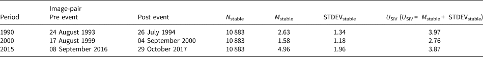
N stable, number of pixels from stable terrain; M stable, mean SIV over selected stable pixels; STDEVstable, std dev. of SIV over stable pixels.
The uncertainties (U SIV) associated with each pair are also given in the table.
The SEC of the Pensilungpa glacier was determined by comparing the AST14 DMO of 2017 and SRTM DEM of 2000. The ASTER DEM was first smoothened using a median filter (3 × 3). Then the peaks and sinks were identified by creating a hillshade image and removed using spline method (Racoviteanu and others, Reference Racoviteanu, Paul, Raup, Khalsa and Armstrong2009; Paul and others, Reference Paul2013). Both the DEMs were coregistered by minimizing the std dev. of the elevation difference over the least error-prone ice-free stable and low sloping areas to achieve horizontal congruence (Berthier and others, Reference Berthier, Cabot, Vincent and Six2016). For this, several masks including glacier mask (GLIMS glacier boundaries for the year 2000; GLIMS, 2015), slope mask (<4° and >45°), cloud mask (manually digitized) and outlier mask (±100 m) were applied on the elevation difference image. After the planimetric adjustment, along/cross track corrections were incorporated by rotating the coordinate system of the ASTER DEM using azimuth of ASTER ground track and estimating elevation difference over stable areas (Nuth and Kääb, Reference Nuth and Kääb2011; Kumar and others, Reference Kumar, Kulkarni, Gupta and Sharma2017). Following this, elevation, slope and curvature-dependent vertical biases were removed from the SEC using all reliable measurements over stable areas (Gardelle and others, Reference Gardelle, Berthier, Arnaud and Kääb2013). During vertical adjustment, the range of outlier mask was narrowed down to ±50 m to have more reliable pixels form stable ground. Table 3 shows the improvement in the std dev. after each correction. The SRTM was created using C-band which potentially underestimates the glaciated terrain due to its varying penetration depth into different glacier classes (i.e. snow, firn, debris), causing one of the most important uncertainty sources (Gardelle and others, Reference Gardelle, Berthier, Arnaud and Kääb2013; Vijay and Braun, Reference Vijay and Braun2016; Zhou and others, Reference Zhou, Li, Li, Zhao and Ding2018). Therefore, to account this error, here we have employed penetration depth correction of 2.3 ± 0.6 m for snow, 1.7 ± 0.6 m for clean-ice and 0.4 ± 0.8 m for debris-covered glacier parts, which is equal to an average penetration depth of ±1.46 m (Kääb and others, Reference Kääb, Berthier, Nuth, Gardelle and Arnaud2012; Gardelle and others, Reference Gardelle, Berthier, Arnaud and Kääb2013; Zhou and others, Reference Zhou, Li, Li, Zhao and Ding2018). Further, the SRTM was acquired in the month of February and the ASTER DEM used here was acquired in the month of September. The potential mass accumulation during these 5 months requires seasonality correction. In the present study, we applied a correction factor of 0.15 m w.e. per winter month as discussed in Gardelle and others (Reference Gardelle, Berthier, Arnaud and Kääb2013) and Zhou and others (Reference Zhou, Li, Li, Zhao and Ding2018). Figure 5 shows the elevation difference before and after the corrections. Finally, the SECs for the concerned glacier were calculated along the central flowline averaged for every 200 m distance from the snout.
Table 3. Statistics of the surface elevation differences on the stable terrain for the raw and corrected difference images
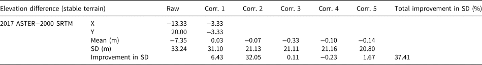
Corrections (Corr.) 1–5 respectively denote the co-registration, spatial trend, elevation, slope, aspect and curvature-related error corrections. The improvement in std dev. (SD) denotes the improvement of each correction compared to the previous step.
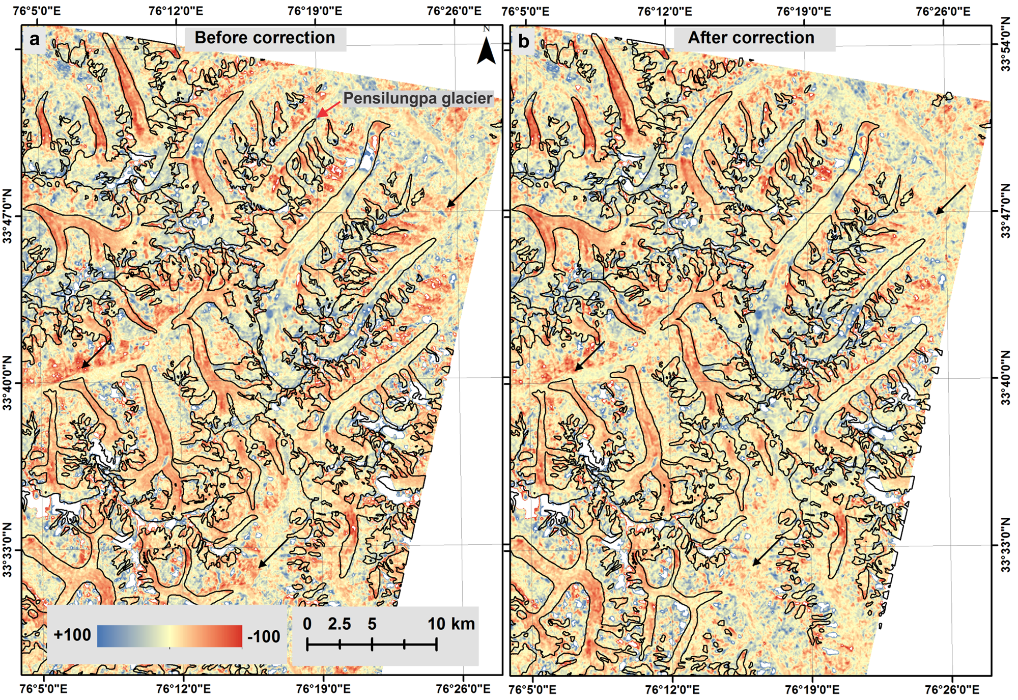
Fig. 5. Map showing (a) raw and (b) corrected elevation difference images deduced by differencing 2000 SRTM DEM from 2017 ASTER DEM. The various corrections include 3-D coregistration, along/across track, elevation, slope and terrain curvature-related error corrections. A good congruence between the temporal DEMs can be seen on stable terrain. Black arrows on the map show sites of improvement. The black polygons show the glacier masks from GLIMS for the year 2000 (GLIMS, 2015; https://www.glims.org/).
3.2. Uncertainty estimation
Quantifying uncertainties associated with remotely derived glacier parameters bears prime importance in substantiating the results (Paul and others, Reference Paul2013; Shukla and Qadir, Reference Shukla and Qadir2016; Kaushik and others, Reference Kaushik, Dharpure, Joshi, Ramanathan and Singh2019). Here, the uncertainties in glacier area and debris cover mapping were estimated using buffer method (Chand and Sharma, Reference Chand and Sharma2015; Garg and others, Reference Garg, Shukla and Jasrotia2019). The buffer size, equivalent to the coregistration error of 6 m (Storey and Chaoate, Reference Storey and Choate2004; Heid and Kääb, Reference Heid and Kääb2012; Bhattacharya and others, Reference Bhattacharya2016), was set. This yielded the uncertainties in glacier area and debris cover estimation as 1.96, 2.02 and 2.10% for 1990 TM, 2000 ETM+ and 2016 OLI.
The uncertainties in temporal area and debris cover changes were quantified as per Hall and others (Reference Hall, Bayr, Schöner, Bindschadler and Chien2003) which comes to ±0.0029 km2 for both the time periods (i.e. 1993–2000 and 2000–16). The uncertainties in snout retreat were also calculated according to Hall and others (Reference Hall, Bayr, Schöner, Bindschadler and Chien2003) which come as ±2.14 m a−1 for 1993–2016, ±6.79 m a−1 for 1993–2000 and ±3.24 m a−1 for 2000–2016 period. The SLA uncertainties can be realized as ±10 m in the vertical (equal to the vertical accuracy of DEM) and ±15 m in the horizontal direction (equal to the buffer size used).
We estimated the uncertainties associated with SIVs as per Scherler and Strecker (Reference Scherler and Strecker2012) and Garg and others (Reference Garg, Shukla, Tiwari and Jasrotia2017) wherein the displacement and std dev. over stable terrain were added and divided by temporal separation of the correlated image-pairs (Table 2). The resultant values varied from ±2.76 m a−1 in 2000 to ±3.97 m a−1 in 1990. Relatively higher uncertainty in 1990 may be attributed to the partial snow and cloud cover in that image. The uncertainty in SEC (U SEC) has been estimated according to Bolch and others (Reference Bolch, Pieczonka and Benn2011) and Bhushan and others (Reference Bhushan, Syed, Arendt, Kulkarni and Sinha2018) using mean (M; −0.14 m) and std dev. (SD; 20.80 m) of elevation difference over stable terrain (number of pixels (n) = 1840471). We first computed standard error (SE) as ${\rm SE} = {\rm SD}/\sqrt n$ to be 0.02 m and then relative error in elevation difference (E SEC) as $E_{{\rm SEC}} = \sqrt {{\rm S}{\rm E}^2 + M^2}$
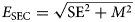 to be 0.14 m. Finally, U SEC was estimated as $U_{{\rm SEC}} = \sqrt {{( {E_{{\rm SEC}}} ) }^2 + {( {E_{\rm p}} ) }^2 + {( {E_{\rm s}} ) }^2}$
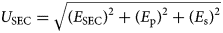 considering the errors in penetration (E p; 0.6 m) and seasonality correction (E s; 0.15 m). Accordingly, the U SEC was computed to be 0.63 m (±0.04 m a−1).
4. Results
4.1. Glacier length, area debris cover and SLA changes
Results reveal that the total length of the Pensilungpa glacier was 8.66 ± 0.03 km in 1993. Over the monitoring period (1993–2016), the glacier retreated at a rate of 6.62 ± 2.11 m a−1 leading to a total length reduction of 152.20 ± 48.43 m. The retreat rate increased from 5.16 ± 6.92 a−1 during 1993–2000 to 7.25 ± 3.03 m a−1 during 2000–16. The glacier area was 15.06 ± 0.28 km2 in 1993 which reduced to 14.89 ± 0.28 km2 in 2000 and further to 14.67 ± 0.29 km2 in 2016. This shows that, in aggregate, the glacier lost 2.56 ± 0.75% (0.11 ± 0.03% a−1) of its total area during the study period.
In 1993, 10.47% (1.58 ± 0.03 km2) of the total glacier area was covered by debris. Accompanying the glacier recession, the supraglacial debris also increased to 15.36% (2.29 ± 0.04 km2) in 2000 and to 17.35% (2.55 ± 0.05 km2) in 2016, revealing an average annual debris growth of 2.86 ± 0.29% a−1. On a decadal timescale, the debris expansion was higher (6.67 ± 0.41% a−1) during 1993–2000, and dropped to 0.81 ± 1.12% a−1 during 2000–16.
The average SLA of the glacier was 5197 ± 73.57 m a.s.l. (std dev. italicized) for the period 1993–2016. As expected, there is significant annual variability in SLA over the study period (Supplementary Fig. S1). Maxima and minima in SLA were attained during 2008 (5310 ± 76 m a.s.l.) and 1993 (5023 ± 20 m a.s.l.), respectively. Overall, the SLA has increased by 137 m in elevation between 1993 and 2016. It can be inferred from the time series SLA that rapid average upshift (between two consecutive years) of 36 m occurred between 1993 and 2000 while SLA descended on an average by 4 m during 2000–2016. Field measurements for the year 2016/17 and 2017/18 suggest the equilibrium line altitude (ELA) to be at 5215 and 5223 m a.s.l., respectively. Field-ELA for 2016/17, though differing from remotely-derived SLA by 56 m, confirms a clear upshift as compared to SLAs of 1993 and 2000. The observed shift between the field and remotely sensed ELAs may be attributed to (a) the difference in the nature of the two, i.e. in field, the elevation representing actual transition between accumulation and ablation is estimated, while using satellite images, the end of season snow line is mapped; (b) the field ELA estimation seldom takes the tributary glaciers into consideration while remotely derived ELA considers the entire boundary between ACZ and ABZ across tributaries.
4.2. SIV and SEC
The SIV of Pensilungpa glacier could only be estimated upto ~5 km distance from snout (Fig. 6a), as the presence of snow in the ACZ resulted in poor correlations. Results reveal that initially (in 1993/94) the glacier was moving with an average speed of 14.23 ± 3.97 m a−1, which reduced to 11.56 ± 2.76 m a−1 in 1999/00 and further to 7.86 ± 3.87 m a−1 in 2016/17. These values are the mean of all reliable measurements obtained for the respective time periods. However, for inter-comparison of temporal SIVs, we have considered only those glacier parts for which good correlations were obtained in all the three time periods. This shows the average SIV to be 13.94 ± 3.97, 9.33 ± 2.76 and 7.63 ± 3.87 m a−1 in 1993/94, 1999/00 and 2016/17, respectively. Thus, the results confirm a total decrease in the glacier velocity by 48.28% (1.97% a−1) between 1993/94 and 2016/17. Spatially, the maximum SIV has been observed in the UAZ (4905–5160 m a.s.l.) or middle part of the glacier while LAZ (4668–4905 m a.s.l.) remained stagnant in all the monitoring periods (Fig. 6a). Further, the SIV for 2016/17 has also been monitored in the field. In total, we could compute field-SIV for 9 stake points located on the LAZ. The average field-SIV is calculated to be 2.81 ± 1.22 m a−1. The remotely-derived SIV for the same year and for the corresponding points is 3.85 ± 3.87 m a−1. Thus, SIV estimates from both approaches reveal very slow movement of the LAZ and, hence, complement each other.
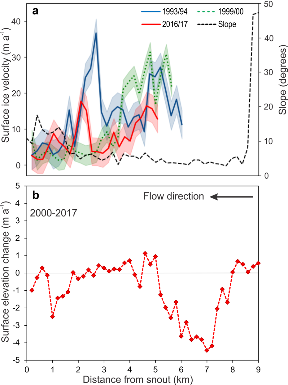
Fig. 6. (a) Surface ice velocity (SIV) of Pensilungpa glacier during 1993/94, 1999/00 and 2016/17 deduced by correlating temporal remote-sensing images, (b) surface elevation change on glacier obtained by subtracting 2000 SRTM digital elevation model (DEM) from 2017 ASTER DEM. Note an almost stagnant condition in the lower ablation zone (upto ~2 km) in panel (a). The stagnant position is also evident in the elevation difference map (panel b). The observed lowering between 1 and 2 km distance from snout may be attributed to the backwasting of ice cliffs.
The glacier SEC has been evaluated between 2000 and 2017 which reveals a thinning of −0.88 ± 0.04 m a−1. We interpret this thinning as predominantly downwasting (see Sections 5.2 and 5.3) and therefore use the term downwasting here as well. The maximum lowering is observed to be concentrated in the UAZ of the glacier (2–5 km upstream from snout) (Fig. 6b). The debris-covered lower portion of the glacier has shown comparatively less lowering. Nevertheless, significant lowering (average −15.75 ± 0.68 m) was noticeable near the snout region, particularly in ~120 m stretch from snout (Fig. 6b), which is likely because of the observed terminal retreat (116 m during 2001–2016) and ongoing processes of cave collapsing near the snout region.
Measurements taken in the field show a clear downwasting (evidenced from nine recovered stakes in 2017) ranging from −0.54 to −1.53 m (average: −0.88 m) during 2016–2017. However, these points mainly covered the lower debris-covered portion of the glacier where the debris thickness is much higher (Fig. 7). During 2017–2018, where the network of stakes was expanded to cover the upper thinly debris-covered portion of the glacier, an enhanced average downwasting of −1.54 m was observed with an incredible downwasting of ~>3 m on stake points where the debris thickness was <5 cm (Fig. 7). The average geodetic lowering on corresponding field points was estimated to be −0.63 ± 0.04 and − 0.71 ± 0.04 m a−1, respectively, which is also in conformity with field-derived downwasting trend and magnitude.
Fig. 7. Debris thickness on Pensilungpa glacier observed in the field during (a) 2016 and (b) 2017. The debris thickness near snout region reaches >40 cm and gradually decreases with increasing distance from snout. Figure also displays the field measured downwasting during 2016–2017 and 2017–2018. Note a clear influence of debris thickness on melting as higher downwasting is evident in upper ablation regions where debris thickness is lower (<5 cm) while less downwasting is apparent in lower ablation regions where debris is thick (~40 cm).
5. Discussion
5.1. Comparison with previous studies
Several past studies have attempted to assess the dimensional changes of the Pensilungpa glacier as well as other glaciers in its vicinity. Table 4 compares the results of length and area change of present study to that of the previous ones. Our length estimates differ considerably from Kamp and others (Reference Kamp, Byrne and Bolch2011) and Pandey and others (Reference Pandey, Ghosh, Nathawat and Tiwari2011). These discrepancies have also been previously recognized by Shukla and Qadir (Reference Shukla and Qadir2016). The study by Kamp and others (Reference Kamp, Byrne and Bolch2011) reported that the Pensilungpa glacier retreated by almost ~1 km (946 m in absolute term) between 1992 and 2006 while Pandey and others (Reference Pandey, Nathawat and Ghosh2012) documented a length change of 693 m during almost the same period (1992–2007). Areal estimates by Ghosh and Pandey (Reference Ghosh and Pandey2013) and Pandey and others (Reference Pandey, Kulkarni and Venkataraman2011) also differ from ours as they spectacle much higher deglaciation (almost double) during the study period (1992–2007). These variations can largely be explained by the inherent quality of data used (e.g. presence of temporal snow cover), obvious difficulties in precisely delineating the debris-covered snout and expertise of the analyst. However, despite differing in magnitude, the reported trend of deglaciation seems in line with the present study which found that the deglaciation rate has reduced post-2000 period (Table 4). Moreover, our results show a good match with Shukla and Qadir (Reference Shukla and Qadir2016). They found that, while retreat rate increased slightly, deglaciation rate of the Pensilungpa glacier reduced significantly during post-2000. These trends are also apparent in our results (Table 4).
Table 4. Comparison of length and area changes of this study with that of previous studies of corresponding study period for Pensilungpa glacier
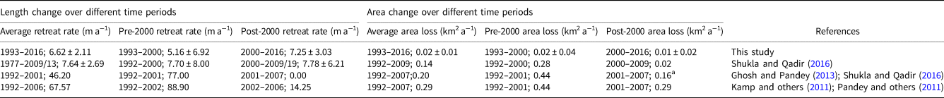
a Increase in glacier area.
In the regional context, the average retreat of the Pensilungpa glacier is lower than that of the other glaciers in the region. Kamp and others (Reference Kamp, Byrne and Bolch2011) monitored 13 glaciers of the Greater Himalaya Range and reported an average retreat of ~20 m a−1 (average of ten glaciers) during 1990–2003, which increased to ~34 m a−1 during 2003–08 (Table 5). They also reported advancement of a few glaciers (e.g. Parkachik). Ali and others (Reference Ali, Shukla and Romshoo2017) assessed 45 glaciers of the Lidder basin and reported an average retreat of 20.6 ± 7.3 m a−1 between 1996 and 2014. Shukla and Qadir (Reference Shukla and Qadir2016) also assessed five glaciers of Suru/Doda basin and noted an average length decrease of 7.8 m a−1. Patel and others (Reference Patel, Sharma, Fathima and Thamban2018) studied 29 glaciers of Miyar basin and found that these glaciers have retreated at a rate of 9.6 ± 5.2 m a−1 between 1989 and 2014. A recent study by Kaushik and others (Reference Kaushik, Dharpure, Joshi, Ramanathan and Singh2019) noted an average retreat of 12.44 ± 3.1 m a−1 during 1979–2017 for the 48 glaciers of Bhaga basin (Table 5). The area loss rate of the Pensilungpa glacier is comparable to the glaciers of the Ravi basin (Chand and Sharma, Reference Chand and Sharma2015) and the Chandra-Bhaga basin (Pandey and Venkataraman, Reference Pandey and Venkataraman2013), but consistently lower than all other monitored basins of the western Himalaya (Table 5).
Table 5. Comparison of retreat and area loss rates of Pensilungpa glacier with those in surrounding basins
NA, not available in the source study; *, retreat (m a−1); †, deglaciation (% a−1).
The SLA monitoring in this study shows a total upshift of 137 m during 1993–2016. However, a notable fluctuation in decadal scale has been observed (Section 4.1). Earlier, Shukla and Qadir (Reference Shukla and Qadir2016) found an average SLA increase of 207 m for the selected five glaciers of Suru/Doda basin and 280 m particularly for Pensilungpa glacier between 1977 and 2011. Thus, our observed SLA trends are in line with these reported measurements. Similar upshifting trends have also been observed in the other basins of western Himalaya (Negi and others, Reference Negi, Saravana, Rout and Snehmani2013; Pandey and others, Reference Pandey, Kulkarni and Venkataraman2013; Garg and others, Reference Garg, Shukla, Tiwari and Jasrotia2017).
The Pensilungpa glacier has also been considered earlier for SIV estimation. Bhushan and others (Reference Bhushan, Syed, Arendt, Kulkarni and Sinha2018) noticed that the lower portion of this glacier (up to ~2 km distance from snout) is nearly stagnant with SIV < 10 m a−1 while upstream portion of main trunk is active (SIV > 10 m a−1). Our results also confirm similar spatial variations wherein the lower parts were found consistently stagnant during all the studied periods whereas upper portion remained active throughout (Fig. 6). Comparison of the temporal velocity variations is restricted by unavailability of such previous measurements on the glacier. However, trends of SIV reduction as observed in this study are comparable to that of previous studies conducted in the nearby basins of the western Himalaya which also report continuous glacier slowdown (Azam and others, Reference Azam2012; Garg and others, Reference Garg, Shukla, Tiwari and Jasrotia2017; Singh and others, Reference Singh2018).
Earlier estimates of SEC demonstrate that the Pensilungpa glacier has been losing mass since 1960s (Pandey and others, Reference Pandey, Ghosh, Nathawat and Tiwari2011; Vijay and Braun, Reference Vijay and Braun2018; Bhushan and others, Reference Bhushan, Syed, Arendt, Kulkarni and Sinha2018). Pandey and others (Reference Pandey, Ghosh, Nathawat and Tiwari2011) found a downwasting ranging from −0.73 to −2.19 m a−1 in the LAZ of this glacier between 1962 and 2003. Recently, Vijay and Braun (Reference Vijay and Braun2018) quantified a downwasting of −0.63 ± 0.10 m a−1 during 2000–2012 for Pensilungpa glacier. In view of this, our SEC results (−0.88 ± 0.04 m a−1) observed between 2000 and 2017 seem to be in line with these measurements. Moreover, regional SEC estimates of −0.66 ± 0.09 m a−1 (2000–2008) by Kääb and others (Reference Kääb, Berthier, Nuth, Gardelle and Arnaud2012) for the entire Jammu and Kashmir, and −0.50 ± 0.28 m a−1 (2000–2012) for the Zanskar region also confirm significant and continuous mass wastage in the study area.
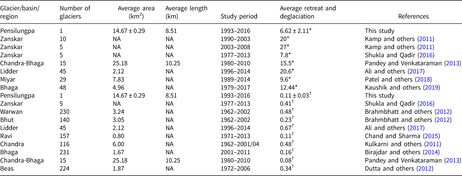
Comparing the spatial map of SEC of Pensilungpa glacier to that of previous studies (Fig. 8), it is evident that our estimates are in accordance with the Pandey and others (Reference Pandey, Ghosh, Nathawat and Tiwari2011), who reported maximum downwasting in the upper ablation area of the glacier and also a slight elevation increase in the lower ablation portion at some places (Fig. 8). Field observation also confirms the presence of several ice mounds on glacier possibly developed due to surface uplift (Fig. 2). Further interpretation of SEC patterns in Figure 8 is provided in Section 5.3.
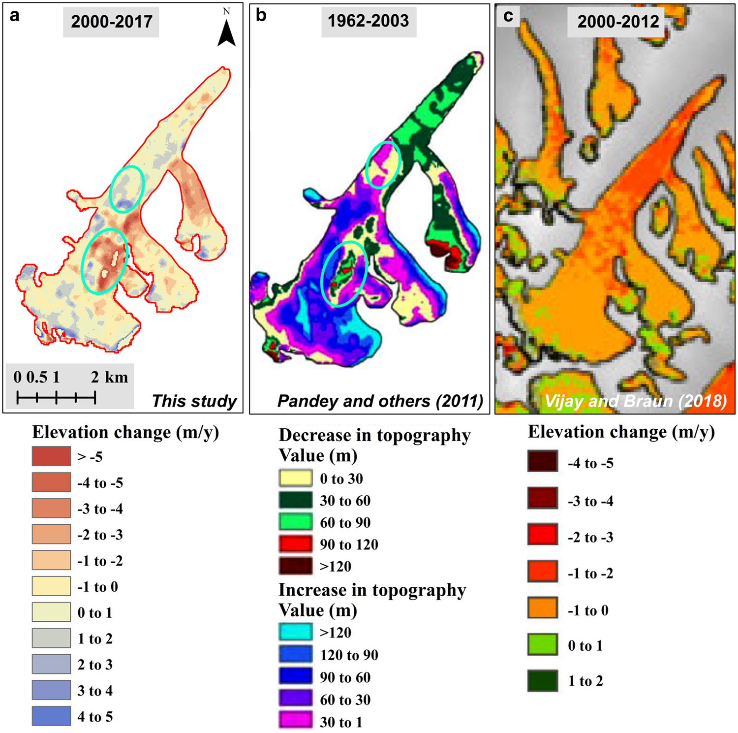
Fig. 8. Comparison of surface elevation changes estimation of this study with the previous studies. Circled areas on panel (a) and panel (b) show a similar trend of elevation change. Large difference in elevation change pattern at lower ablation zone may be due to large difference in the study periods and presence of debris cover (thickness >10 cm) which grew (by ~66%) during the study period (1993–2016) and exerting insulating effect. Permissions were obtained from Springer and Elsevier to reprint the figures from Pandey and others (Reference Pandey, Ghosh, Nathawat and Tiwari2011) and Vijay and Braun (Reference Vijay and Braun2018), respectively.
Moreover, we have observed higher lowering near the junction of right bank tributary glaciers to the main trunk which is also evident in the spatial SEC map of Pandey and others (Reference Pandey, Kulkarni and Venkataraman2013) (Fig. 8). Our spatial SEC map deviates from Vijay and Braun (Reference Vijay and Braun2018) which shows slightly higher downwasting (in order of −1 to −2 m a−1) in the middle ablation portion. This deviation may be due to redistribution of ice mounds in this portion as observed during the field visits, which indeed gives the impression of elevation increase. Nevertheless, averaged downwasting over the entire glacier estimated by Vijay and Braun (Reference Vijay and Braun2018) study is comparable to our estimations.
5.2. Glacier stagnation: evidence
Results of almost all the monitored parameters including length, area, debris cover, SLA, SIV and SEC indicate toward a depleting pattern of the Pensilungpa glacier during 1993–2016 (Sections 4.1 and 4.2). Climate trends reveal a clear rise in the mean annual temperature (0.77°C) and considerably high increase in the mean annual minimum temperature (1.3°C) over the last century. The temperature rising trend further accelerated over the last two to three decades (Shukla and others, Reference Shukla, Garg, Mehta, Kumar and Shukla2020). A recent study by Mehta and others (Reference Mehta, Kumar, Garg and Shukla2021) linked depleting pattern of the Pensilungpa glacier to this temperature rise. However, assessment on decadal scale reveals that the glacier wastage was higher during 1993–2000 which subsequently reduced in the time frame 2000–16. The relative area loss rate was lower (0.09 ± 0.09% a−1) during 2000–16 as compared to 1993–2000 (0.17 ± 0.24% a−1). Slowdown rates were also higher during 1993/94–1999/00 (4.73% a−1) as compared to 1999/00–2016/17 (1.14% a−1). Here, results of SLA reveal a sharp ascend of snowline (180 m) during 1993–2000 indicating a low accumulation during this period which possibly led to higher deglaciation and drastic dropdown in the SIV. However, during 2000–2017, the SLA descended only by 43 m which is in compliance with observed reduction in slowdown and deglaciation rates. In synchronization with deglaciation and SIV, the debris-growth rate was also significantly higher during 1993–2000 (6.67 ± 0.41% a−1) followed by a steep cut (0.09 ± 0.09% a−1) during 2000–2016. During recession, as the glacier ice melts, debris mantle over it is left behind leading to an increase in the spatial extent of debris (Thompson and others, Reference Thompson, Benn, Mertes and Luckman2016; Ali and others, Reference Ali, Shukla and Romshoo2017). Here the only exception is snout retreat parameter which, in contrast to prevailing trend of generalized slowdown of glacier depletion rate, increased slightly in the recent decade (2000–16: 7.25 ± 3.03 m a−1) as compared to the previous one (1993–2000: 5.16 ± 6.92 m a−1). This increase in the retreat rate appeared to be induced by terminus environment and may not be directly linked to climate. This is explainable as an active dry-calving (break-off of ice blocks) and collapse of the ice-cave ceilings (due to undercutting by the sub-glacial waters and related seepage) have been observed in snout portion during all the field visits (Fig. 9). Large ice blocks are continuously being detached from the glacier in this part (Fig. 9). Hence, it appears that these dry calving and ice-cave collapse have probably led to slightly higher retreat in the recent decade. Further, it may be noted that the current and dominant process of ablation in the glacier is downwasting. In this study, downwasting has only been calculated for the 2000–17 period. However, comparing with Pandey and others (Reference Pandey, Ghosh, Nathawat and Tiwari2011) who have calculated extensive downwasting on this glacier (−0.76 to −2.19 m a−1) during 1992–2003, it can be asserted that the SEC rates have also reduced after 2000. These multiparametric observations confirm that the glacier is heading toward stagnation. Also, the spatial distribution of SIV elucidates that the lower portion of the glacier (up to ~1.5 km distance from the snout) has become almost stagnant.
Fig. 9. Snout characteristics of the Pensilungpa glacier. A large cave can be seen at the snout of this glacier where frequent activities of dry calving (i.e. direct breaking-off of ice blocks) have been observed during the field visits. Field photographs are of the year 2017.
5.3. Glacier stagnation: causes
Glacier stagnation results from a chain of processes: firstly, an inadequate snow supply/mass input into the glacier (evident from ascending SLA) leads to glacier slowdown, downwasting and deglaciation (dimensional reduction) (see Sections 4.1 and 4.2). Downwasting and deglaciation result in an accumulation of debris on the glacier surface (Ali and others, Reference Ali, Shukla and Romshoo2017; Garg and others, Reference Garg, Shukla, Tiwari and Jasrotia2017; Section 4.1). Here, the SIV plays a major role in redistribution, mobilization and removal of debris cover from the glacier system (Schroder and others, Reference Shroder, Bishop, Copland and Sloan2000; Quincey and others, Reference Quincey, Luckman and Benn2009). Reduced glacier velocities negatively impact the efficient debris transfer mechanism of the glacier and hence the debris cover gradually thickens and expands up-glacier. Thus, the continuous increase of debris cover during 1993–2016 (2.86 ± 0.29% a−1) and greater debris thickness near the snout region (>40 cm) indicate that these processes are active on the glacier.
The debris thickness distribution, though heterogeneous, largely follows a common pattern such that the debris thickness (a) increases from central flowline toward margins and (b) decreases with increasing distance from snout (Anderson and Anderson, Reference Anderson and Anderson2018). Our field observations also confirm a very thick debris cover (~40 cm) near the snout regions and thin debris-covered patches (2–5 cm) on up-glacier side. The debris thickness plays a major role in regulating the melt rates. Field measurements show comparatively low downwasting near the snout region of the Pensilungpa glacier where the debris is thick while higher downwasting has been observed over bare ice (covered with debris dust) and on the regions where debris thickness is generally less (Fig. 7). Here, we have also quantified the correlation between debris thickness and downwasting. A good correlation coefficient (r 2 = 0.51) between debris thickness measured in 2016 and downwasting during 2016–2017 was found (Fig. 10a). Similarly, an improved correlation (r 2 = 0.56) between debris thickness and downwasting during 2017–2018 has been observed (Fig. 10b). These findings further confirm a significant influence of the debris thickness on melt rates.
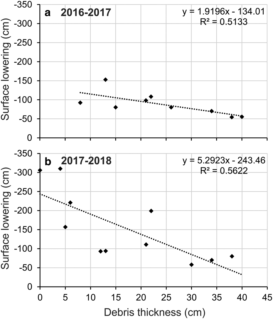
Fig. 10. Correlation between debris thickness and downwasting observed on the field during (a) 2016–17 and (b) 2017–18. The correlation is apparently negative which implies that higher the debris thickness lower the downwasting.
Given the influence of the debris thickness on melting, the observed debris thickness distribution has the following implications. Firstly, the thick debris cover probably protected the glacier margins which is the most likely reason of observed reduction in deglaciation rates of the Pensilungpa glacier in the recent decade. Eventually, thick debris cover, stable/insulated glacier margins and the impedance created by the side valley-walls collectively contributed in dragging the glacier velocity down, which lead to stagnation of lower portion of the glacier. Secondly, the observed distribution of the debris thickness has promoted a characteristic inverted ablation gradients (Figs 6b, 7) on the glacier which have long been recognized as one of the prime factors underpinning the distinct/unique response of the debris-covered glaciers (Scherler and others, Reference Scherler, Bookhagen and Strecker2011; Benn and others, Reference Benn2012; Sharma and others, Reference Sharma2016). This inverted ablation coupled with the decrease in glacier thickness reduced the driving stress (Quincey and others, Reference Quincey, Luckman and Benn2009; Benn and others, Reference Benn2012), which causes further stagnation. Figure 8 also shows a shift in SEC trends at LAZ over the time. Though the different color gradients and the different units in panels (a) and (b) of Figure 8 make direct comparison difficult, it can be asserted that the magnitude of lowering at LAZ was slightly higher during 1962–2003 (Pandey and others, Reference Pandey, Ghosh, Nathawat and Tiwari2011). However, owing to notable insulating effect of debris, the lowering rates have reduced in the recent period (2000–2017). Moreover, owing to progressive reduction in velocity (as evident by the current trend of slowdown) and continued downwasting, the stagnant zone is likely to extend further up.
5.4. Stagnation: implications on glacio-geomorphic processes and resulting ice cliffs
Annual field measurements show a pronounced location melting on the glacier in the recent years, i.e. for 2016–17 and 2017–18 (Fig. 7). Geodetic measurements also confirm a notable average downwasting of −0.88 ± 0.04 m a−1 between 2000 and 2017. Interestingly, in spite of this observed overall downwasting, long-term SEC calculations (2000–17) reveal almost no net change in overall surface elevation in glacier parts 2–5 km up-glacier and even a slight surface uplift has been noticed (Fig. 6). Earlier, Thomson and others (Reference Thompson, Benn, Mertes and Luckman2016) also noticed striping of downwasting alternating with the areas of apparent uplift, with values up to ±50 m during 2010–12 and 2012–15 on the Ngozumpa glacier of Nepal. They stressed that the striped pattern is the resultant of displacement of surface topography down-glacier by ice flow. Here, evaluating our results in light of velocity results, it is evident that uplift has occurred on dynamically active part (i.e. ~2–5 km from snout) directly up-glacier of the lower stagnant zone. We interpret it as bulging-up of ice mass in this region, possibly induced by contrasting velocities of active upper portion and stagnant lower region which balances the melting of ice resulting in no net change in overall surface elevation.
The slow moving (<10 m a−1) and gently sloping (<6–8°) glacier tongue, supported by prevailing negative mass-balance regimes, forms favorable conditions for the formation and development of the glacial lakes and ice cliffs (Sakai and others, Reference Sakai, Nakawo and Fujita2002; Miles and others, 2016; Thompson and others, Reference Thompson, Benn, Mertes and Luckman2016). On the Pensilungpa glacier, a few supraglacial ponds have been observed (Fig. 4) which, though small in size, are likely to expand rapidly due to expected melting of dusty ice-walls surrounding the ponds (Benn and others, Reference Benn, Wiseman and Hands2001; Sakai and others, Reference Sakai, Nakawo and Fujita2002). Moreover, the Pensilungpa glacier is riddled with ice cliffs. Here, a detailed assessment of lower tongue (~2 km upstream) has been carried out using high-resolution images from GoogleEarthTM (Centre National d'Études Spatiales (CNES), France/Airbus) for 2013 and 2017 to assess the dynamics of these ice cliffs (Fig. 11). Visual inspection of this portion shows no sign of movement. Most of the surface features have been preserved during 2013–2017. For instance, well-identifiable big boulders present on the surface remained stationary between 2013 and 2017 confirming stagnant state of underlying ice. These observations corroborate well with the results obtained by correlating Landsat images (Fig. 6) in this study. However, the only notable activity in this portion is the backwasting of ice cliffs. Ice cliffs are the typical features of debris-covered glaciers (Sakai and others, Reference Sakai, Nakawo and Fujita2002; Benn and others, Reference Benn2012). The average melt rate at an ice cliff has been reported to be ~10 times that of debris-covered areas (Sakai and others, Reference Sakai, Nakawo and Fujita1998, Reference Sakai, Nakawo and Fujita2002). Earlier, several studies have highlighted significant contribution of ice cliffs on total mass wastage of a glacier which may range from ~8 to 40% even they occupy small fraction of total glacier area (Sakai and others, Reference Sakai, Nakawo and Fujita1998, Reference Sakai, Nakawo and Fujita2002; Immerzeel and others, Reference Immerzeel2014; Thomson and others, Reference Thompson, Benn, Mertes and Luckman2016). In the present study, we digitized all the ice cliffs present on the lower ~2 km portion interactively on high-resolution images from GoogleEarthTM for the years 2013 and 2017. Results show a total number of 52 ice cliffs with a total area of 33 854 m2 in 2013. In 2017, the total number and area of ice cliffs increased significantly to 77 and 47 607 m2, respectively. It is important to note that the dark shadows caused by steep ice cliffs make it challenging to demarcate their borders precisely even on the high-resolution images and may introduce sizable error. However, a clear increase of ~48% in number and 41% in area of ice cliffs within such a short period of time (i.e. ~4 years) clearly indicates that the backwasting of ice cliffs is the dominant mechanism of mass loss in this portion.
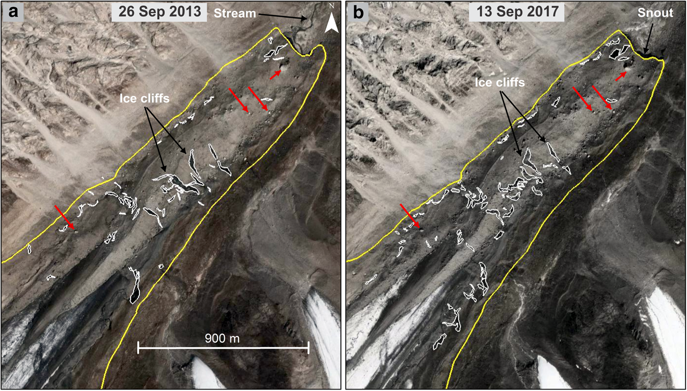
Fig. 11. Temporal evolution of lower ablation zone (~2 km upstream) between (a) 2013 and (b) 2017, observed using high-resolution images from GoogleEarthTM (Centre National d'Études Spatiales (CNES), France/Airbus) dated 26 September 2013 and 13 September 2017, respectively. The stagnant state of this portion is evident from the stationary position of the supraglacial markers (boulders; marked by red arrows) during 2013–2017. Progressive development of ice cliff is also apparent on the temporal images which suggests that an active back-wasting process is operative on the glacier.
6. Conclusions
This study has attempted to assess the present conditions as well as the evolution of the Pensilungpa glacier during 1990–2017. For this, multiple glacier parameters namely length, area, debris cover, debris thickness, SLA, SIV, SEC and ice cliffs were evaluated using field and remote-sensing data acquired between 1993 and 2017. The results show that, though the depletion rate is comparatively lower as compared to the other western Himalayan glaciers, the glacier is in depleting phase with a clear reduction in almost all the monitored glacier parameters, with a notable increase in SLA and concomitant growth in debris cover area during 1993–2016. A clear temperature increase (especially in mean annual minimum temperature) in the study region over the last century and particularly over the last two to three decades seems to be the prime driver of observed glacier changes. However, overall glacier wastage rate has reduced in the recent time period (2000–17) as compared to the previous one. From the results, it has been inferred that a comparatively less SLA upshift during 2000–17 and remarkable debris area and thickness increase during 1993–2000 might be the probable reasons of this reduction in depletion rates. Further, the SIV results confirm that the LAZ (up to 2 km up-glacier) has remained stagnant during the study period. The debris thickness characteristics of the glacier can be largely ascribed to this stagnation.
The thickness of the supraglacial debris gradually decreases from the snout up-glacier and from the margins to the central flowline. Such debris thickness distribution has not only insulated the glacier margins but also contributed in observed slowdown. Further, debris thickness-induced differential melting (i.e. less downwasting near snout region and high downwasting up-glacier) has resulted in characteristic slope inversion, which also contributed in the stagnation by reducing the driving stress. Stagnation has had several implications: First, lower stagnant ablation portion has caused slight bulging in the upper dynamically active part of ABZ. Second, slow moving debris-covered zone has facilitated the development of supraglacial ponds which are low in number and small in extent but are likely to grow in future. Third, numerous ice cliffs developed on the lower ablation portion (up to ~2 km up-glacier). Systematic assessment of these ice cliffs between 2013 and 2017 reveals a marked increase in their number and area. Thus, given the insulated glacier margins and reducing glacier velocities, back-wasting of ice cliffs dominates the ablation process in the glacier.
Supplementary material
The supplementary material for this article can be found at https://doi.org/10.1017/jog.2021.84
Acknowledgement
The authors are thankful to the Director, Wadia Institute of Himalayan Geology for providing required facilities to carry out this work. A.S. thanks the Secretary, Ministry of Earth Sciences, Government of India for facilitating the study. The authors extend sincere gratitude to Dr Hester Jiskoot (Associate Chief Editor), Dr Neil Glasser (Scientific Editor) and the two anonymous referees whose detailed comments have significantly improved the paper. P.K.G. acknowledges the research grant from National Post-Doctoral Fellowship (NPDF) award (PDF/2020/000103) from the Department of Science and Technology, Government of India and the Indian Institute of Technology Indore, India for hosting NPDF tenure.
Author contributions
P.K.G. and A.S. designed the study and wrote the paper. P.K.G. performed calculations and generated the figures. S.G. and B.Y. estimated field-velocity. V.K., M.M., A.S. and S.G. contributed to field measurements. All the authors discussed the results and contributed to the final form of the article.


 Open access