


1. Introduction
Turbulent detrainment is observed in a variety of environmental and laboratory flows, yet its origin and mechanism have not been clearly elucidated. While turbulent plumes have long been characterised by the entrainment of ambient fluid with Kelvin–Helmholtz-type (K-H) engulfing eddies near the turbulent/non-turbulent perimeter, it is only relatively recently that detrainment has been observed for plumes generated adjacent to a vertical wall or cylinder emitting a nominally uniform buoyancy flux in a confined environment such as a filling box (Cooper & Hunt Reference Cooper and Hunt2010; Gladstone & Woods Reference Gladstone and Woods2014; Bonnebaigt, Caulfield & Linden Reference Bonnebaigt, Caulfield and Linden2018). For both wall and cylinder cases, turbulent detrainment, manifesting as intermittent ejections of fluid filaments from the plume into the environment, occurs in the stably stratified region and several wedge-like intrusions form. Apart from wall plumes, cumulus clouds as well as gravity currents overlying inclined substrates in stratified media have also been observed to exhibit simultaneous entrainment and detrainment along their perimeters (Taylor & Baker Reference Taylor and Baker1991; Baines Reference Baines2001). Thus, enhancing our modelling capability of detrainment in plumes has potentially wide benefits.
One of the proposals for the detrainment mechanism is based on the ‘plume peeling’ description (Hogg et al. Reference Hogg, Dalziel, Huppert and Imberger2017). Since the plume buoyancy is non-uniform in the cross-stream direction, when the outermost layer of the lowest buoyancy reaches its neutral level, it ‘peels off’ from the plume and intrudes horizontally into the ambient. Incorporating this process into a wall plume model, such as that of Cooper & Hunt (Reference Cooper and Hunt2010), leads to an improved qualitative prediction of the stratification pattern in a filling box (Bonnebaigt et al. Reference Bonnebaigt, Caulfield and Linden2018). However, the above description of plume peeling regards a turbulent plume as a coflow of multiple laminar layers and, therefore, may oversimplify the fluid exchange between the plume and environment. Moreover, the turbulent entrainment process that is still significant for a detraining plume (Gladstone & Woods Reference Gladstone and Woods2014) is not accounted for.
In the present work, we adopt an alternative description of detraining plumes, one which is centred on quantifying the simultaneous entrainment and detrainment with an entrainment and a detrainment coefficient, respectively. A detrainment coefficient approach can be readily incorporated into the classic Morton–Taylor–Turner (MTT) plume model (Morton, Taylor & Turner Reference Morton, Taylor and Turner1956), and the solutions for detraining plumes compared with those for purely entraining plumes (Hunt & van den Bremer Reference Hunt and van den Bremer2011) in order to gain wider insight into the impact of detrainment on plume behaviour. In this description, the fluid exchange at the plume perimeter is viewed as a sequence of intermittent lateral entrainment and detrainment fluxes. This mirrors an approach by Baines (Reference Baines2001) in the study of gravity currents on slopes. While the entraining motions originate from the vorticity wave, or the K-H wave, associated with an inflectional vertical velocity profile, detrainment occurs due to the interaction, referred to as the Holmboe mechanism (Parker, Caulfield & Kerswell Reference Parker, Caulfield and Kerswell2020), of this wave with an internal wave (due to the stable stratification across the sloping plume boundary) within the plume. Such an internal wave can only be sustained if the offset between the points of maximum lateral gradients of vertical velocity and buoyancy is sufficiently large, or equivalently, if the thickness difference between the vertical velocity and buoyancy profiles is sufficiently small. It is worth noting that the Holmboe mechanism referred to above is a conceptual analogy to the classic case where the internal wave develops along a horizontal density interface.
To achieve the flow regime with detrainment, the flow configuration must therefore support the Holmboe mechanism, which, according to the above discussion, corresponds to a sufficiently small ratio  $\lambda$ of the buoyancy and vertical velocity thicknesses. For free plumes, this ratio, defined in the sense of the $1/e$-thicknesses, has been reported from measurements to approximate to a universal value exceeding unity, e.g. $\lambda \approx 1.3$ for line plumes (Paillat & Kaminski Reference Paillat and Kaminski2014). However, this ratio substantially drops to $\lambda \approx 0.34$, as evaluated from figure 7 of Parker et al. (Reference Parker, Burridge, Partridge and Linden2021), for a wall plume generated by a plane vertically distributed buoyancy source. Clearly, this reduced ratio of thicknesses is due to the wall-shear resistance which results in significantly flatter vertical velocity profiles relative to those of free plumes. The presence of a wall qualitatively changes the mixing regime, with locally either pure entrainment or both entrainment and detrainment at the plume perimeter. We therefore restrict the focus of this study to plumes bounded by a wall, but it should be borne in mind that detrainment may also be achieved by other factors that result in sufficiently small values of $\lambda$.
Besides the wall effect, an essential condition for the detraining plume regime appears to be a sufficiently strong ambient stratification. In the filling-box experiments which exhibited plume detrainment (Cooper & Hunt Reference Cooper and Hunt2010; Gladstone & Woods Reference Gladstone and Woods2014; Bonnebaigt et al. Reference Bonnebaigt, Caulfield and Linden2018), the horizontal interface, that delineates the unstratified and stably stratified regions of the environment, partitions exactly the detraining and non-detraining regions of the wall plume. The mechanism that governs how a strong stratification contributes to detrainment may be related to the region of flow reversal and negative buoyancy at the plume perimeter (Tao, Le Quéré & Xin Reference Tao, Le Quéré and Xin2004; Yu & Hunt Reference Yu and Hunt2023). While the negative buoyancy can be directly related to the peeling of an outer plume layer (Hogg et al. Reference Hogg, Dalziel, Huppert and Imberger2017), both the flow reversal and negative buoyancy phenomena become increasingly significant when the gradient of the ambient buoyancy is enhanced. In their description of simultaneous plume entrainment and detrainment, Yu & Hunt (Reference Yu and Hunt2023) reasoned that wall plume detrainment is caused by the absolute instability which is commonly associated with flow reversal and negative buoyancy, and a strong ambient stratification (Tao et al. Reference Tao, Le Quéré and Xin2004).
The remainder of this article is organised as follows. In § 2, the simultaneous detraining and entraining plume formulation is established with the key coefficients modelled with simplified relations. The profiles and characteristic quantities of detraining plumes are then analysed and a comparison with traditional plumes made in § 3. Conclusions drawn from the new understanding garnered from this distinct detraining plume regime and regarding the applicability of the modelling framework innovated herein are given in § 4.
2. Plume model with simultaneous entrainment and detrainment
Consider a statistically steady and two-dimensional turbulent plume rising vertically along a wall emitting a uniform buoyancy flux per unit area of  $\chi$ ( ${\rm m}^2\,{\rm s}^{-3}$) in a stably stratified quiescent miscible fluid medium. The basic situation, with nomenclature and coordinate system $(y,z)$, is depicted in figure 1. Unless stated otherwise, all flow quantities relating to the plume are time averages. With $\rho (y,z)$, $\rho _a(z)$ and $\rho _r=\mathrm {const.}$ referring to the plume, ambient and reference densities, respectively, the plume buoyancy is defined as ${\phi (y,z)=g(\rho _a-\rho )/\rho _r}$ and the ambient buoyancy as ${\phi _a(z)=g(\rho _r-\rho _a)/\rho _r}$, where $g$ is the gravitational acceleration. While both $\phi (y,z)$ and the vertical plume velocity $w(y,z)$ are assumed to adopt ‘top-hat’ cross-stream profiles so that either quantity is uniform within a lateral boundary and zero outside, the interfaces at which they become zero are defined as $y=\lambda b(z)$ and $y=b(z)$, respectively, where $\lambda$ is a constant. Due to the wall-shear resistance, the value of $\lambda$ is significantly below unity, see § 1 and the supporting data in Parker et al. (Reference Parker, Burridge, Partridge and Linden2021).

Figure 1. Schematic of a simultaneously entraining and detraining wall plume with top-hat cross-stream profiles in a stably stratified quiescent environment with natural, or buoyancy, frequency  $N(z)$. The buoyant layer of width $\lambda b(z)$ is shown in grey. The perimeter of the vertical velocity layer of width $b(z)$ and velocity $w(z)$ is represented by the dashed line.
Both the entrainment and detrainment are taken to occur at the plume perimeter  ${y=b(z)}$. At a given elevation $z$, the (laterally inward) entrainment velocity $u_e$ and (laterally outward) detrainment velocity $u_d$ are assumed to be proportional to the local characteristic vertical plume velocity. Thus, with $\alpha _e$ and $\alpha _d$ denoting the entrainment and detrainment coefficients, respectively,
 \begin{equation} u_e=\alpha_e w\quad \mathrm{and}\quad u_d=\alpha_d w. \end{equation}
The physical reasoning behind the linear  $u_d(w)$-relation above is that similar to entrainment, detrainment is enhanced by more significant turbulent eddies, characterised by a higher inertia. The entrainment coefficient for a classic purely entraining free line plume, $\alpha _{e,free}$, has been well-established as (van den Bremer & Hunt Reference van den Bremer and Hunt2014)
 \begin{equation} \alpha_{e,free}(Ri)=\gamma_1+\gamma_2 Ri, \end{equation}
where  $\gamma _1$ and $\gamma _2$ are empirical constants, and the local Richardson number $Ri$ is
 \begin{equation} Ri= \frac{BQ^3}{2\alpha_{e,eq} M^3}, \end{equation}
where  ${Q=wb}$, ${M=w^2b}$ and ${B=\lambda \phi wb}$ are the plume volume, specific momentum and buoyancy fluxes along the vertical direction, respectively, and $\alpha _{e,eq}$ the coefficient of entrainment in the far field in an unstratified environment. For simplicity, we assume that the entrainment coefficient for a wall plume is a constant fraction $c_w$ of that for a free line plume, i.e. ${\alpha _e(Ri)=c_w \alpha _{e,free}(Ri)}$, where $c_w$ is referred to as the coefficient of entrainment loss (relative to one half of a free line plume). Combining ${\alpha _{e,free}(Ri=1)=0.11}$ (Richardson & Hunt Reference Richardson and Hunt2022) for a pure line plume and $\alpha _{e,free}(Ri=0)=0.05$ (Antonia et al. Reference Antonia, Browne, Rajagopalan and Chambers1983) for a line jet yields the $\alpha _e(Ri)$ dependence for a wall plume
 \begin{equation} \alpha_e(Ri)=c_w(0.05+0.06Ri). \end{equation}
 The precise dependencies of the detrainment coefficient  $\alpha _d$ on the flow configuration and local parameters are still in question. Nevertheless, the detrainment coefficient should be an increasing function of the buoyancy gradient in the environment ${N^2(z)=\mathrm{d} \phi _a(z)/\mathrm{d} z}$ according to the observations of Gladstone & Woods (Reference Gladstone and Woods2014) and Bonnebaigt et al. (Reference Bonnebaigt, Caulfield and Linden2018), and have a certain dependence on the local plume properties via $Ri(z)$. Moreover, from the work of Gladstone & Woods (Reference Gladstone and Woods2014) it is evident that there exists a critical natural frequency $N_{cr}$ for which the detrainment flux equals the entrainment flux, i.e. $\alpha _d= \alpha _e$ at $N= N_{cr}$, and, as such, there is zero net inflow or outflow. Accordingly, with $\mathcal {H}$ denoting the Heaviside step function, the following simple linear constitutive relation on $N^2$ is adopted that captures this behaviour:
 \begin{equation} \alpha_d(Ri,N^2)/\alpha_e(Ri)=\mathcal{H}(N-N_{min})\left[(N^2-N^2_{min})/(N^2_{cr}-N^2_{min})\right], \end{equation}
where  $N_{min}$ is the threshold natural frequency above which detrainment occurs. For simplicity, we take ${N_{min}=0}$ with ${N\geq 0}$ and the above relation simplifies to
 \begin{equation} \alpha_d(Ri,N^2)/\alpha_e(Ri)={N}^2/N_{cr}^2. \end{equation}
Caution should be taken when applying the detrainment model (2.5) to certain special flow regimes, e.g. the flow near the horizontal intrusion of which the outflow complicates the picture of detrainment. As outlined in § 1, while entrainment is a result of engulfing K-H eddies, detrainment is achieved via thin fluid filaments ejected into the ambient. For the present model, we assume that such filaments are absorbed instantaneously into the vast ambient without affecting the ambient buoyancy  $\phi _a(z)$. Consequently, the ambient fluid that is entrained into the plume can always be regarded as being neutrally buoyant and, thereby, as having no effect on the plume buoyancy flux.
Under the standard assumptions for Boussinesq plumes (which neglect diffusion, see Morton et al. Reference Morton, Taylor and Turner1956), the conservation relations are (see also Baines Reference Baines2001)
 \begin{equation} \frac{\mathrm{d} Q}{\mathrm{d} z}=q+(\alpha_e-\alpha_d)\frac{M}{Q},\quad \frac{\mathrm{d} M}{\mathrm{d} z}=\frac{BQ}{M}-\frac{\tau}{\rho_r}-\alpha_d \frac{M^2}{Q^2},\quad \frac{\mathrm{d} B}{\mathrm{d} z}={-}Q\frac{\mathrm{d}\phi_a}{\mathrm{d} z}+\chi-\alpha_d\frac{BM}{Q^2}. \end{equation}
The source term  $q(z)$ represents the volume flux per unit height supplied to the plume from the wall, e.g. due to the ablation of a submerged ice wall or supply of saline solution, and is neglected hereinafter. The lateral blowing force associated with this source volume flux, which may marginally enhance detrainment, is also neglected. The term ${\tau =c_f\rho _r w^2}$ (Kaye & Cooper Reference Kaye and Cooper2018) denotes the wall-shear stress. Based on the measurements of McConnochie & Kerr (Reference McConnochie and Kerr2016) for meltwater plumes from the vertical face of an ice wall and the analysis of Kaye & Cooper (Reference Kaye and Cooper2018), we take ${c_f=0.54}$. Compared with classic plumes, a simultaneously entraining–detraining plume is characterised by the extra volume, momentum and buoyancy terms with the coefficient $\alpha _d$, which indicate physically the losses of vertical fluxes due to lateral ejections of rising plume masses.
With the superscript  $({\cdot })^*$ indicating the dimensionless variable, the scalings are chosen as follows and serve to reduce (2.7a–c) to the simplest form:
 \begin{equation} \left.\begin{gathered} Q=( N_{cr}^{{-}2}\chi)Q^*,\quad M=N_{cr}^{-({5}/{2})}\chi^{{3}/{2}}M^*,\quad B= N_{cr}^{-({3}/{2})}\chi^{{3}/{2}}B^*,\\ z=N_{cr}^{-({3}/{2})}\chi^{{1}/{2}}z^*,\quad N=N_{cr} N^*. \end{gathered}\right\} \end{equation}
The corresponding scalings for the plume width, vertical velocity and buoyancy are  ${(b,w,\phi )=(N_{cr}^{-({3}/{2})}\chi ^{{1}/{2}}b^*}, {N_{cr}^{-({1}/{2})}\chi ^{{1}/{2}}w^*}, {N_{cr}^{{1}/{2}}\chi ^{{1}/{2}}\phi ^*})$. Substituting (2.8a–e) into (2.7a–c) and omitting the superscript $({\cdot })^*$ for convenience, the dimensionless conservation relations are
 \begin{equation} \frac{\mathrm{d} Q}{\mathrm{d} z}=(\alpha_e-\alpha_d)\frac{M}{Q},\quad \frac{\mathrm{d} M}{\mathrm{d} z}=\frac{BQ}{M}-(\alpha_d+c_f) \frac{M^2}{Q^2},\quad \frac{\mathrm{d} B}{\mathrm{d} z}={-}N^2 Q+1-\alpha_d\frac{BM}{Q^2}. \end{equation}
Hereafter, all variables considered are dimensionless. We focus on linear ambient stratifications, i.e. with  ${N^2=\mathrm {const.}}$, and expect that the results are more widely applicable given that a general ambient stratification may in principle be approximated as being piecewise linear. The system (2.9a–c), once the constant $c_w$ is prescribed, is fully characterised by the dimensionless ambient buoyancy gradient ${N^2}$, and can be solved with the ‘leading-edge’ condition ${(Q=Q_0,M=M_0,B=B_0)}$ at $z=0$. If all fluxes are zero at the leading edge, a condition that represents a reference physical situation, the numerical integration encounters a singularity at ${z=0}$. To address this issue, we add to the leading-edge condition a small artificial perturbation which guarantees small and positive gradients of the flux quantities around ${z=0}$. According to our tests, ${(Q_0,M_0,B_0)=(10^{-4},10^{-6},0)}$ is an appropriate choice and imposing such a perturbation does not change the plume solution except in the immediate vicinity of ${z=0}$.
2.1. Determination of the coefficient of entrainment loss
At this stage, information is still required on the actual value of the coefficient of entrainment loss,  $c_w$, in the $\alpha _e(Ri)$ dependence (2.4). In principle, $c_w$ can be determined by substituting the value of any known $(\alpha _e,Ri)$ pair into (2.4). Although McConnochie & Kerr (Reference McConnochie and Kerr2016) measured that ${\alpha _{e,eq}=0.05}$ in the far field of a solely entraining wall plume in an unstratified environment, there has been no available experimental data for the corresponding equilibrium Richardson number $Ri_{eq}$.
Substituting  ${\alpha _e=0.05}$ into (2.4), the equilibrium Richardson number is $Ri_{eq}=5(1/c_w-1)/6$. This expression is plotted in figure 2 as the solid line labelled $Ri_{eq,1}$. Alternatively, by prescribing $c_w$ and solving numerically the system (2.9a–c) with zero leading-edge fluxes and ${N^2\equiv 0}$, the equilibrium Richardson number can be acquired with its definition (2.3). This solution is plotted as the dashed line labelled $Ri_{eq,2}$. These two estimations of the equilibrium Richardson number for the unstratified case must be identical. Evidently, the point of intersection of the two curves suggests the actual value of the coefficient of entrainment loss as ${c_w=0.12}$ and the equilibrium Richardson number as ${Ri_{eq}=6.0}$. It should be borne in mind that the coefficient $c_w$ varies with wall roughness and can be regarded as a property of the wall and, thus, while the present methodology and conclusions are applicable for general wall plumes, the above numerical values of $c_w$ and $Ri_{eq}$ are those for plumes along a vertical surface of ice.

Figure 2. The far-field equilibrium Richardson number vs the coefficient of entrainment loss  $c_w$ for a wall plume in an unstratified environment acquired either by the expression ${Ri_{eq}=5(1/c_w-1)/6}$ (the solid curve, ${Ri_{eq,1}}$) or the numerical solution of (2.9a–c) (the dashed curve, ${Ri_{eq,2}}$).
3. Characteristics of detraining plumes
3.1. Detraining effect and dynamic quasi-equilibrium
When the environment changes from unstratified ( ${N^2=0}$) towards strongly linearly stratified ( ${N^2=1}$), the detrainment flux increases from zero towards being equal to the entrainment flux, i.e. $\alpha _d/\alpha _e$ increases from $0$ to $1$. The wall-plume profiles for four representative cases, ${N^2=\{0,0.25,0.5,0.75\}}$, in this entrainment-dominated regime are plotted in figure 3. Zero fluxes at ${z=0}$ are prescribed, which leads the plume to achieve a dynamic equilibrium, or a balanced state with streamwisely similar flow situations, immediately above the leading edge, so as to exclude the near-field adjustment stage.

Figure 3. Dimensionless solutions for zero leading-edge fluxes. (a) Width, (b) vertical velocity, (c) buoyancy, (d) volume flux, (e) specific momentum flux and (f) buoyancy flux. The arrow indicates increasing  $N^2$ or stronger detraining effects for ${N^2=0}$ (solid), $0.25$ (dot-dash), $0.5$ (dashed) and $0.75$ (dotted). The grey circle in (d) marks where the solution is singular.
It is apparent from figure 3 that, except for the unstratified case where the plume rises indefinitely with a linear spread, a detraining plume spreads near linearly and then at an ever-increasing gradient  $\mathrm{d} b/\mathrm{d} z$, before intruding horizontally about its neutral height (e.g. the $N^2=0.5$ dashed line in figures 3a and 3c). Since linear plume spreading usually corresponds to a dynamic equilibrium with self-similarity, we propose that the approximate linearity here indicates a dynamic quasi-equilibrium or slowly drifting self-similar state (Kaminski, Tait & Carazzo Reference Kaminski, Tait and Carazzo2005). This is confirmed later with reference to a local Richardson number invariance. Over the vertical range in which this quasi-equilibrium persists, with $N^2$ increasing, the detrainment is enhanced and, consequently, the plume width shrinks relative to the less strongly stratified cases. Meanwhile, the fluxes of volume, specific momentum and buoyancy all increase with height at reduced rates, together with slower vertical motions ( $w$ increasing less rapidly).
At elevations above the quasi-equilibrium region, the detraining plume undergoes a radical change in behaviour in which the flow as a whole adjusts towards intruding horizontally, resulting in a rapid breakdown of the quasi-equilibrium. In the vertical domain depicted in figure 3, only the  ${N^2=0.5}$ case exhibits a horizontal intrusion. The intrusion corresponds to a singularity (the grey circle in figure 3d) of the $Q$-profile at the initial discharge height ${z=z_{int}}$, a height defined such that ${w(z_{int})=0}$. Beyond the discharge height, due to the continual buoyancy gain, the wall plume is expected to reform with a zero source volume flux and the above process recurs (Yu & Hunt Reference Yu and Hunt2021). It appears that above a threshold height, at some distance below ${z=z_{int}}$, the breakdown of quasi-equilibrium is accompanied by an accelerated reduction of $M$ and $B$ with height towards zero, whereas the volume flux $Q$ continues to increase, albeit at a reduced rate.
From figure 4(a), as the ambient stratification is enhanced,  $z_{int}$ first decreases and then increases. While the plume rises indefinitely for both the unstratified ( ${N^2=0}$) and zero-net-inflow ( ${N^2=1}$) cases, the minimum of $z_{int}$ is achieved at ${N^2\approx 0.5}$. Much as for classic purely entraining plumes, a weak or moderate stratification ( ${N^2<0.5}$) promotes the formation of a lower horizontal intrusion since, with an enhanced ambient stratification, the rising buoyant fluid reaches the neutral level at lower heights. Nevertheless, for sufficiently large ${N^2\ ({>}0.5)}$, the ambient stratification significantly delays the onset of an intrusion, resulting in it forming at greater heights; the physical reason behind this peculiar behaviour is that stronger detrainment restricts the growth of the volume flux – in other words, there is less dilution of the plume fluid relative to that achieved for a lower $N^2$. Therefore, with a given wall buoyancy flux, the plume (of reduced volume flux or width) remains more buoyant and thereby intrudes at a higher level.

Figure 4. (a) Dimensionless initial discharge height vs the ambient buoyancy gradient. (b) The vertical evolution of the local Richardson number  ${Ri=BQ^3/(2\alpha _{e,eq} M^3)}$.
It is of great interest how a detraining wall plume can exhibit a dynamic quasi-equilibrium, behaviour which is indicated by a slow vertical variation of the local Richardson number. We therefore plot, see figure 4(b), the  $Ri(z)$-profiles for various $N^2$. Clearly, the local Richardson number is almost uniform along $z$ with ${Ri\approx 6.0}$ below the heights at which the plume begins the transition into a horizontal intrusion. This quasi-equilibrium $Ri$ has a very weak dependence on $N^2$, which implies that the same flow regime or dynamical balance is always achieved, irrespective of the ambient stratification. The local $Ri$ drops rapidly towards zero over the transitional region, whose occurrence depends on $N^2$ in the same manner as revealed earlier in the discussion accompanying figure 3. While the slow variation of $Ri$ in the quasi-equilibrium range suggests weakly non-similar plume profiles, the breakdown of the dynamic quasi-equilibrium in the transitional range indicates rapid streamwise ‘degeneration’ of the local plume profiles. Interestingly, over a region below the threshold height (e.g. ${20\lesssim z\lesssim 40}$ for ${N^2=0.5}$, from figures 3b and 3d), the vertical velocity appears almost invariant and the volume flux variation approximately linear. Since ${b\sim z}$ and ${Ri\sim z^0}$ for the quasi-equilibrium region, insisting ${w\sim z^0}$ yields the following power-law solutions in this intermediate region:
 \begin{equation} \phi\sim z^{{-}1},\quad Q\sim z, \quad M\sim z,\quad B\sim z^0, \end{equation}
which is reminiscent of the similarity solution in Caulfield & Woods (Reference Caulfield and Woods1998) for a marginal free plume state which is also between unbounded and bounded states.
3.2. Near-field adjustment: plume swelling and necking
In the filling-box experiments (e.g. Cooper & Hunt Reference Cooper and Hunt2010), there is a non-zero volume flux  $Q_0$ at the height of the first front (the leading edge), and thus, the near-field behaviour of plume adjustment becomes significant. An important observation on detraining plumes concerns the modulation effect of the ambient buoyancy gradient on, what we shall refer to as, the plume swelling and necking phenomena. Given we have established ${Ri_{eq} \approx 6}$ as the equilibrium state for a detraining wall plume, dynamically lazy plume behaviour and, potentially, necking are to be anticipated for ${Ri(z)>Ri_{eq} \approx 6}$, and forced plume behaviour for ${Ri(z)< Ri_{eq} \approx 6}$. Figure 5 plots the dimensionless variation of plume width with height for leading-edge Richardson numbers
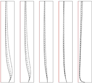
  ${Ri_0=Ri(z=0)}$ that span four decades.

Figure 5. The near-field evolution of plume width for various ambient buoyancy gradients:  ${N^2=0}$ (solid), $0.25$ (dot-dash), $0.5$ (dashed) and $0.75$ (dotted) when ${Q_0=M_0=1}$. Here (a) ${B_0=0.01}$; (b) ${B_0=0.1}$; (c) ${B_0=0.6}$; (d) ${B_0=1}$; (e) ${B_0=10}$.
Peculiarly, for  ${Ri_0< Ri_{eq}}$ (figure 5a,b), a detraining wall plume swells rapidly immediately downstream of the leading edge to form a wedge-like perimeter, after which it contracts and tends towards the far-field behaviour shown in figure 3. The swelling phenomenon becomes more apparent for decreasing $Ri_0$, and is significantly enhanced by a stronger ambient stratification. While swelling has never been reported in any study of classic plumes, the present detraining plume formulation allows a plume with a deficit of buoyancy flux, or ‘forced wall plume’, to swell and contract during the adjustment to equilibrium. The wedge-like plume perimeters reported in the filling-box experiments of Gladstone & Woods (Reference Gladstone and Woods2014) and Bonnebaigt et al. (Reference Bonnebaigt, Caulfield and Linden2018) may be attributed to this swelling mechanism which potentially dominates in the vicinity of a fresh-saline interface.
From figure 5(d,e), for which  ${Ri_0>Ri_{eq}}$, the same necking mechanism as that for free lazy plumes (Hunt & Kaye Reference Hunt and Kaye2005) is preserved for the ${Ri_0=100}$ case, but not obviously apparent for the ${Ri_0=10}$ case where the plume simply contracts. Thus, similar to free plumes, there exists a ‘necking Richardson number’ ${Ri_{neck}\ (>Ri_{eq})}$ above which a lazy wall plume dynamically adjusts with a necking envelope. While the necking phenomenon is enhanced with increasing $Ri_0$, a higher ambient buoyancy gradient $N^2$ also tends to promote plume necking, see figure 5(e). The equilibrium case ( $Ri_0=6$), for which the adjustment region is negligible, is plotted in figure 5(c) for comparison, and interestingly, the plume only marginally contracts beyond the leading edge.
Moving forward, the picture we have gained of the detraining wall plume (summarised on the right-hand side of figure 1), is thus one comprising three regions, each with distinct behaviours, a near-field adjustment, a quasi-equilibrium and a transitional region.
4. Conclusion
By incorporating an empirically modelled detrainment coefficient, our detraining wall plume formulation for stratified environments predicts rich dynamical behaviours that have not been theorised previously. One outstanding feature, in accordance with filling-box experiments, is the remarkable wedge-shaped plume envelope predicted for non-equilibrium ‘forced’ conditions at the leading edge. Moreover, far beyond the leading edge a region of dynamical quasi-equilibrium is established which breaks down rapidly at greater elevations as the plume transitions to a horizontal intrusion.
Compared with the unstratified case, a weak stratification prompts the plume intrusion to occur at lower levels, whereas for sufficiently strong stratifications ( ${N^2>0.5}$), the plume intrudes at increasingly higher levels. Further refinements on the present model would rely considerably on acquiring experimentally the exact relations $\alpha _d(N^2,Ri)$ and $\alpha _e(Ri)$ for wall plumes, a notoriously formidable task with the current technologies. While we assume a linear dependence of the ratio of $\alpha _e$ to $\alpha _d$ on the ambient buoyancy gradient (2.5), the constitutive relation for $\alpha _d$ may be more complex in reality. Nevertheless, any new version of $\alpha _d(N^2,Ri)$ can in principle be adapted into the theoretical framework established herein. We expect this modelling approach to be applied as a complement of the classic MTT theory in cases where the Holmboe mechanism alters the Kelvin–Helmholtz mechanism and the outflow due to detrainment cannot be neglected.
Acknowledgements
The authors gratefully thank three anonymous referees for their helpful comments on an earlier draft.
Declaration of interests
The authors report no conflict of interest.


 Open access