


1. Introduction
Electric vehicle energy replenishment relies on charging stations. In the parking lot, the area occupied by parking places with charging stations is larger than that of regular parking spaces, which reduces the utilization rate of the parking lot. Many parking lots do not have charging stations because electric vehicles were not yet widely used during construction. At the same time, the charging process of electric vehicles still requires manual operation, including plugging and unplugging the charging gun. People need to transfer the vehicle to a regular parking space after the electric vehicle is charged, because the cost of charging a parking space is higher than that of a regular parking space. The proposal of mobile charging robots proposed by companies such as Volkswagen and Tesla has solved the above problems. It has the functions of autonomous navigation and more complete charging operations. After receiving the electric vehicle charging command for the target parking space, the mobile charging robot moves to the vicinity of the vehicle to complete the charging operation and returns to the robot cabin or goes to the next parking space after the electric vehicle charging is completed. The schematic diagram of the mobile charging robot module is shown in Fig. 1(a), and its working process is shown in Fig. 1(b).

Figure 1. Sketch map of mobile charging robot.
Mobile robot systems are roughly divided into information perception, path planning, and motion control [Reference Liu, Wang, Yang, Liu, Li and Wang1]. Among them, path planning is to find a collision-free safe path from the current position to the target position within a specified range for the robot after obtaining corresponding environmental and task information, thereby guiding the robot’s movement. The iteration and length of path planning affect the reaction time, running time, and wear of the robot. For mobile charging robots, path planning typically involves the robot cabin to the parking space of the electric vehicle that needs to be charged. Path planning can be divided into global path planning and local path planning based on the information of environment [Reference Li, Huang, Ding, Song and Lu2–Reference Xiaofei, Yilun, Wei, Hui, Weibo and Zhengrong3]. This article only analyzes the static parking environment and studies the path planning of mobile charging robots, which belongs to global path planning. For parking lot environments, the environmental information includes fixed channels and empty and occupied parking spaces. The randomness of the occupied parking spaces for parked vehicles and the frequent entry and exit of vehicles result in a high degree of complexity in path planning and also easy to lead to C-space obstacles, which is a major challenge in path planing [Reference Chen4]. Different from fixed obstacle environments for storage robots, the path planning of mobile charging robots in parking lots needs to be able to quickly respond to different obstacle environments, which puts higher requirements on iterations and stability of path planning algorithms.
The path planning algorithm includes two parts: environment modeling and path search. Common methods for environmental modeling include grid method, topological method, and geometric characteristic method [Reference Liu, Wang, Yang, Liu, Li and Wang1]. Howden et al. [Reference Howden5] proposed grid method in 1968, which divides the environment into grids of the same size and stores obstacle information in the grid. The size of the grid method determines the resolution of the environment and the detail of the path: when the grid size is large, the path planning time is shorter, but the planned path will be longer, and the low resolution of the environment will cause the paths that can pass to be impassable; when the grid size is large, the path is shorter, but the path planning algorithm takes up a lot of computation and storage space, and an increase in the number of iterations leads to a longer path search time. Zhang et al. [Reference Zhang, Wang, Fang and Yuan6] proposed a multilevel humanoid motion planning method based on Laser Range Finder (LRF) two-dimensional grid graph, taking into account the multiple constraints of robot and environment to guide robot autonomous navigation in unstructured indoor environment; Raouf et al. [Reference Raouf, Mohammed, Mohammad, Tamer and Maamar7] use vision and image processing algorithms to extracted the obstacle position information and build the 2D grid map; Shao et al. [Reference Shao, Zheng, Wei, Guo, Yang, Wang and Zhao8] established square grid maps and cellular grid maps to address the issue of uneven step size in traditional grids.
The topological method uses nodes to represent a specific position and edge to represent the connections between these positions [Reference Chien, Zhang and Zhang9]. Gomez et al. [Reference Gomez, Fehr and Millane10] proposed a global topology representation of large-scale indoor scenes, where each room is modeled as a submap of the topology map for robot navigation and trajectory planning; Shin and Kim [Reference Shin and Kim11] proposed an algorithm to improve the optimality of planning MPP (Multi-Agent Path Planning) solutions through parallel pebble plots.
The geometric characteristic method refers to a mobile robot that extracts relatively abstract geometric features, such as lines, arcs, and circles, from environmental perception information to describe the environment [Reference Guivant, Nebot and Durrant-Whyte12]. Liang et al. [Reference Xiao, Guanglei, Yimin and Haitao13] proposed a GCM-based path planning method for unmanned aerial vehicles. This method focuses on the shape of obstacles and ultimately finds a collision-free path. These obstacles are organized in a tree list.
The environment of the parking lot is regular, with parking spaces arranged in sequence. By using the grid method and selecting an appropriate grid size, the shortest path can be obtained while ensuring fast iteration of the path planning algorithm.
According to the characteristics of the algorithm, scholars divide it into: (a) classic algorithm; (b) meta-heuristic algorithm; and (c) artificial intelligence algorithm. Classical algorithms are prone to generate high computational cost and low computational efficiency; artificial intelligence algorithms require a lot of data for model training. Compared with these two algorithms, the meta-heuristic algorithm has low computational cost and simple structure and can get approximate solutions in a short time.
In the past 5 years, meta-heuristic algorithms have been proposed to solve various research problems, such as Wang [Reference Wang14] proposed the Moth Search Algorithm (MSA) inspired by the phototaxis of moths; Heidari et al. [Reference Heidari, Mirjalili, Faris, Aljarah, Mafarja and Chen15] proposed the Harris Hawks Optimization (HHO) algorithm inspired by the cooperation and pursuit behavior of the Harris Hawk Group; Wang et al. [Reference Wang, Deb and Cui16] proposed the Monarch Butterfly Optimization (MBO) algorithm inspired by the migration of monarch butterflies; Li et al. [Reference Li, Chen, Wang, Heidari and Mirjalili17] proposed the Slime Mold Algorithm (SMA) inspired by the osculation mode of slime mold in nature; the Colony Prediction Algorithm (CPA) proposed by Tu et al. [Reference Tu, Chen, Wang and Gandomi18] inspired by the corporate prediction of animals in nature; Yang et al. [Reference Yang, Chen, Heidari and Gandomi19] proposed the Hunger Games Search (HGS) algorithm inspired by the general purpose population based optimization technique; Ahmadianfar et al. [Reference Ahmadianfar, Heidari, Noshadian, Chen and Gandomi20] proposed the weighted mean of vectors algorithm (INFO) inspired by the weighted mean idea; and Su et al. [Reference Su, Zhao, Heidari, Liu, Zhang, Mafarja and Chen21] proposed the rime optimization (RIME) algorithm by the physical phenomenon of rime ice. However, compared to the Gray Wolf Optimization (GWO) algorithm, further research is needed on these meta heuristic algorithms in path planning problems.
Zhang et al. [Reference Zhang, Zhou, Li and Pan22] demonstrated in his 2016 research on drone paths that GWO algorithm has faster iteration speed and shorter path length compared to the Cuckoo Search (CS) algorithm [Reference Yang and Deb23], the Flower Pollination Algorithm (FPA) [Reference Yang24], the Novel Bat Algorithm (NBA) [Reference Meng, Gao, Liu and Zhang25], the Bird Swarm Algorithm (BSA) [Reference Meng, Gao, Lu, Liu and Zhang26], the Artificial Bee Colony (ABC) algorithm [Reference Karaboga and Basturk27], and the Gbest-guided Grabitational Search Algorithm (GGSA) [Reference Mirjalili and Lewis28]; Kumar [Reference Kumar, Singh and Tiwari29] demonstrated in his study on path planning for the autonomous robots that the GWO algorithm has faster iteration speed and shorter path length compared to the Particle Swarm Optimization (PSO) [Reference Wang and Cai30] and the Improved Bat Algorithm (IBA) [Reference Guo, Gao and Cui31]; Qu [Reference Qu, Gai, Zhang and Zhong32], Panda [Reference Panda, Das and Pati33], and Radmanesh [Reference Radmanesh, Kumar and Sarim34] demonstrated the superiority of GWO algorithm over the Simulated Annealing (SA) algorithm [Reference Kazemi, Abdul-Rashid, Ariffin, Shekarian and Zanoni35], the Symbiotic Organisms Search (SOS) algorithm, the Ant Colony Optimization (ACO) algorithm [Reference Aghababa36], and the Genetic Algorithm (GA) [Reference Mirjalili, Mirjalili, Lewis and Optimizer37]. Therefore, this article chooses the GWO algorithm as the research object for path planning of mobile charging robots in parking lots.
Through the analysis of references, in order to address its shortcomings, the improvement of GWO mainly includes the following aspects: population initialization, convergence factor, and position update function. Zhang Zhu et al. generated more population samples through chaotic mapping [Reference Zhu, Shenghua and Shijie38]; Wang Xiao improved GWO (IGWO) by combining Logistic-chaotic mapping and heuristic path fine-tuning operator, which improved the local development ability of the algorithm [Reference Xiao39]; Liu Zhiqiang et al. expanded the initial population sample through Tent-chaotic mapping and adjusted the convergence factor and control parameters [Reference Zhiqiang, Li, Liang and Heng40]. Among them, Li Su used the A* algorithm to search in 32 neighborhoods and 48 directions during population initialization, improving the success rate and richness of the path, which inspired this article [Reference Su and Yourui41]. After further research on the A* algorithm, it was found that it not only improves GWO algorithm in population initialization, but also in algorithm iteration and position update functions, to a greater extent avoiding falling into local optima.
The defining feature of the A* algorithm is to establish a “Closed List” to record the evaluated areas, an “Edge List” to record those areas that have already been evaluated, and to calculate the distance from the “Starting Point” to the estimated distance to the “Target Point” [Reference Liu, Wei, Li and Wang42–Reference Ma, Zhao, Li, Yan, Bi and Królczyk44]. This article applies this method to the iteration and position update process of GWO algorithm, partially solving the problem of falling into local optima. The research content of this part is presented in Section 3.3.
This article first analyzes the grid size of the grid method in the parking lot in Chapter 2; secondly, according to the established parking lot model, GWO algorithm of mobile charging robot path planning is improved in fitness function, convergence factor, and location update function; then, the IGWO algorithm was further improved by integrating the A* algorithm in fitness function in Chapter 3; finally, simulation verification was conducted on the fused improved A*-IGWO in different capacity parking lots and different parking lot occupancy rates in Chapter 4.
2. Mapping
2.1. Grid method
The terrain of the parking lot is regular, with fixed passage areas, making it suitable to use the grid map method for map establishment. The schematic diagram of the parking lot setup in this article is shown in Fig. 2(a), and the dimensions of the parking lot are shown in Fig. 2(b). The parking area is divided into 6 areas, with a total of 49 parking spaces. The mobile charging robot cabin is located in the upper left corner of the map. To ensure the normal operation of the mobile charging robot, its parking position should be on one side of the charging socket in front of the required charging vehicle. The S-grid represents the starting point of the path for the mobile charging robot cabin, white represents the parking lot passage, which is the accessible area for the robot. The black grid represents the used parking space, which is an obstacle. The gray grid represents the unused parking space, which is also the accessible area for the robot. And the red represents the vehicle that needs to be charged. The T-grid represents the stopping position of the mobile charging robot, which is the path termination point. The path of a mobile charging robot should start from the starting point, pass through a passable area, and avoid obstacles to reach the termination point.

Figure 2. Sketch diagram of parking lots.
2.1.1. Program
The algorithm process for grid parking lot maps is as follows:
STEP 1 Build grid interface size: number of rows and columns.
STEP 2 Define the entire domain of the grid map and initialize blank areas.
STEP 3 Setting up parking lot road areas and parking space areas.
STEP 4 Randomly generate obstacles (cars) in the parking space area.
STEP 5 Set the starting point (robot cabin) and target point (near the vehicle to be charged) of the mobile charging robot.
STEP 6 Draw a grid map of the parking lot.
For grid maps, the grid coordinates in the i row and j column are (i, j), and the recorded data is 0 in the case of obstacles, and 1 in the case of accessible conditions, stored in map variables.
2.1.2. Size of grid
The grid sizes of the map are 2.60 × 2.60 m2, 1.30 × 1.30 m2, and 0.65 × 0.65 m2, respectively, with corresponding map grids of 10 × 15, 20 × 30, and 40 × 60. Using the GWO algorithm, path planning was performed on maps with three different obstacle situations (vehicle parking conditions). The relationship between the number of iterations and path length is shown in Fig. 3, and the path planning results are shown in Fig. 4. The CPU model of the simulation experimental platform is AMD R7 3700X, and the memory is 8 GB × 4 2666 Hz, operating system is Windows 10, and software platform is MATLAB R2021b.
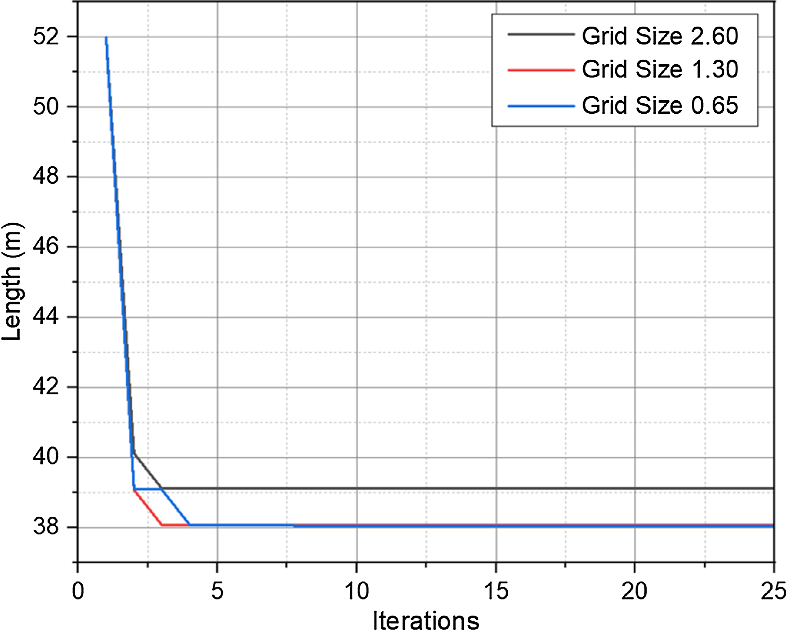
Figure 3. Simulation results of different grid size.

Figure 4. Path planning results of different grid size.
The simulation results show that a map with a grid size of 2.60 × 2.60 m2 has the least number of iterations but the longest path length when using the traditional GWO algorithm for path planning; The grid size of 0.65 × 0.65 m2 has the highest number of iterations, but the shortest path length. The number of iterations for maps with a grid size of 1.30 × 1.30 m2 has increased by an average of 0.5 compared to maps with a grid size of 2.60 × 2.60 m2, which is less than 10%, but the path length has been shortened by more than 2.9%, which is 1.12 m. Compared to maps with a grid size of 0.65 × 0.65 m2, the average number of iterations has decreased by 4.72, which is greater than 171.6%, while the path length has increased, which is less than 0.1%. Therefore, selecting a grid size of 1.30 × 1.30 m2 can meet the requirements of both speed and path length for the path planning algorithm.
2.2. Testing map
The test map is designed to test the robustness, iterations, and path length of the algorithm, as shown in Fig. 5. Wherein, Fig. 5(a) is the schematic diagram of the test map, and Fig. 5(b) is the gird map of the test map, with the grid size of 1.3 × 1.3 m2.

Figure 5. The test map.
For simulations, the parking lots map is a randomly generated obstacle test map in a 52 × 78 m2 parking lot, as shown in Fig. 6, with a grid size of 1.3 × 1.3 m2.

Figure 6. The grid map of parking lots.
3. Algorithm
3.1. GWO
GWO algorithm was first proposed by Mirjalili et al. in 2014 and is an optimization algorithm based on the hunting process of gaey wolf packs [Reference Zhu, Shenghua and Shijie38]. GWO algorithm is a swarm intelligence optimization algorithm based on the hunting behavior of the gray wolf and social stratum. The wolf has a strict hierarchy. The pyramid of the gray wolf class is shown in Fig. 7. Alpha wolf pack is the head wolf class in the population, responsible for leading the pack and making decisions; Beta wolf pack is the subordinate of the Alpha wolves, responsible for assisting Alpha wolves make decisions and manage wolf packs; Delta wolf pack is the executor responsible for completing the decisions made by Alpha wolves and Beta wolves; Omega wolf pack is responsible for observing and balancing relationships in the wolf pack.

Figure 7. The pyramid of the gray wolf class.
The hunting process of wolf packs involves tracking, chasing, and approaching prey; chasing, surrounding, and harassing prey until it stops moving; and attacking prey. In GWO algorithm, the alpha wolf and beta wolf, delta wolf guidance at the same time omega wolves approach their prey and then rescreen based on their relative position to the prey alpha wolf, beta wolf, and delta wolf, then iterate through the loop, as shown in Fig. 8. For path planning problems, the optimization goal of GWO is path length, which is achieved by iterating continuously to obtain the optimal path node and connecting the nodes to obtain the path. GWO algorithm has the advantages of simple structure, easy coding, and fewer parameter settings. However, in terms of path planning, traditional GWO have problems such as a lack of diversity in the initial population and being prone to falling into local optima, which affects the accuracy of the algorithm, leads to collisions between robots and obstacles, and reduces the efficiency.

Figure 8. Sketch diagram of gray wolf hunting.
In the traditional GWO algorithm, alpha wolf, beta wolf, and delta wolf are the first, second, and third optimal solutions of the problem, respectively, and guide omega wolves to find the best optimal solution, and then update the status of the wolf pack. The evolution process of the GWO algorithm is such as Eqs. (1)–(4):
 \begin{equation} D=\left| C\cdot X_{P}\!\left(t\right)-X\!\left(t\right)\right| \end{equation}
 \begin{equation} C=2\cdot r_{1} \end{equation}
 \begin{equation} A=2a\cdot r_{2}-a \end{equation}
 \begin{equation} a=2\cdot \left(1-\frac{t}{T}\right) \end{equation}
where D is the distance between the individual gaey wolf and the target; C is the distance adjustment coefficient; Xp (t) is the target position; X(t) represents the individual position of the gray wolf; X(t + 1) updates the position of gray wolf individuals based on the position of the previous generation of gray wolves; A is the position adjustment coefficient; r 1 and r 2 are uniformly distributed random variables on [0,1]; a is the convergence factor; t is the current number of iterations; and T is the maximum number of iterations.
According to Eqs. (1)–(4), it can be inferred that the hunting target is alpha wolf, beta wolf, and delta wolf. The target positions X 1(t), X 2(t), and X 3(t) observed by wolves are shown in Eqs. (5)–(7), respectively, to guide the wolf pack in approaching the hunting target, as shown in Eq. (8):
 \begin{equation} X_{1}\!\left(t\right)=X_{\alpha }\!\left(t\right)-A\cdot D_{\alpha } \end{equation}
 \begin{equation} X_{2}\!\left(t\right)=X_{\beta }\!\left(t\right)-A\cdot D_{\beta } \end{equation}
 \begin{equation} X_{3}\!\left(t\right)=X_{\delta }\!\left(t\right)-A\cdot D_{\delta } \end{equation}
 \begin{equation} X\!\left(t+1\right)=\frac{X_{1}\!\left(t\right)+X_{2}\!\left(t\right)+X_{3}\!\left(t\right)}{3} \end{equation}
where X $_{\alpha}$
(t), X
$_{\alpha}$
(t), X $_{\beta}$
(t), and X
$_{\beta}$
(t), and X $_{\delta}$
(t) for
$_{\delta}$
(t) for ${\alpha}$
wolf,
${\alpha}$
wolf, ${\beta}$
wolf, and
${\beta}$
wolf, and ${\delta}$
wolf, respectively; D
${\delta}$
wolf, respectively; D $_{\alpha}$
, D
$_{\alpha}$
, D $_{\beta}$
, and D
$_{\beta}$
, and D $_{\delta}$
are the distance between the wolf and the target.
$_{\delta}$
are the distance between the wolf and the target.
Generally, if the individual position of a gray wolf is the fitness function value of the solution, then the fitness function L of path planning is shown in Eq. (9):
 \begin{equation} L=\sum\nolimits_{k=1}^{k=\dim }\sqrt{\left(x_{k+1}-x_{k}\right)^{2}+\left(y_{k+1}-y_{k}\right)^{2}} \end{equation}
where dim is the problem dimension, which is the total number of path nodes; k is the number of path nodes that the path passes through, xk is the X-direction coordinate of the k-th path node, and yk is the coordinate of the k path node in the Y-direction. The fitness function value L is the total length of the path, which is accumulated by the distance between adjacent path nodes.
For robot path planning, each gray wolf individual stores path node information. During the evolution process, the path nodes approach the shortest path, and it is necessary to determine whether there are obstacles between adjacent path nodes. The basic steps of the traditional GWO algorithm are as follows:
Step 1 Initialize the population and generate a random path from the starting point to the ending point.
Step 2 Determine whether there are obstacles in the connection between each adjacent path node of the gray wolf individual, calculate the fitness function value (path length), and filter ${\alpha}$
wolf,
${\alpha}$
wolf, ${\beta}$
wolf, and
${\beta}$
wolf, and ${\delta}$
wolf.
${\delta}$
wolf.
Step 3 Update the convergence factor a, position adjustment coefficient A, and distance adjustment coefficient C.
Step 4 According to alpha wolf, beta wolf, and delta wolf based on the path information provided by the omega wolves, plan each path node again to determine whether the termination condition is met. Otherwise, return to Step 2.
Step 5 Satisfies the termination condition and outputs ${\alpha}$
. The path information of the wolf is used as the optimal path.
${\alpha}$
. The path information of the wolf is used as the optimal path.
3.2. IGWO
3.2.1. Fitness function
In the study of the GWO algorithm, path planning found that the path is affected by the number of path node, path node generally set for developers, violates the principle of the shortest distance between two points, the fitness function value is affected by the path node number at the same time, generally will increase the final optimization results of the algorithm. Zhuo et al. (2018) use RimJump to decrease the number of path node in A* and Dijkstra algorithm, which inspire us [Reference Zhuo, Weimin, Yongliang, Mingzhu, Zhenshuo, Fangxing and Qiang45].
In order to solve this problem, this article adopts the interpolation method to further optimize the results of the path planning and make the path smoother. The specific steps are as follows:
Step 1 Obtain the optimized path node set.
Step 2 Determine thesequence whether there are obstacles between the two nodes.
Step 3 Filter out the minimum path nodes that can reach the target location.
Step 4 Interpolate the filtered nodes based on their distance according to the dimensions of the path node set.
Step 5 Output the optimized path node set and fitness function value (total path length).
3.2.2. Location update function
The schematic diagram of the position update function principle is shown in Fig. 9. During the operation of the traditional GWO algorithm, Eqs. (5)–(8), the path nodes of omega wolves can be determined based on alpha wolf, beta wolf, and delta wolf. The omega wolves’ path node information was ultimately averaged, resulting in three paths bypassing the same obstacle from different directions. The calculated average of the path nodes was located within the obstacle, as shown in Fig. 9(a), resulting in the failure of the path planning algorithm. To solve this problem, this article has changed the calculation method of path nodes, using the results optimized by the GWO algorithm as the guidance direction for iterative nodes, as shown in Fig. 9(b), to guide the robot forward and generate a new path. The specific steps are as follows.

Figure 9. Location update.
Step 1 Initialize the robot position with a path node dimension of dim.
Step 2 Calculate the first optimized path node based on the GWO algorithm.
Step 3 Determine whether the k-optimized path node is an obstacle.
Step 4 The robot advances in the direction of the k-th optimized path node until encountering obstacles. Otherwise, the robot advances to the position of the k-th optimized path node and records it as the k-th path node.
Step 5 calculates the (k + 1)-th optimized path node based on the GWO algorithm and returns to Step 2 until the robot advances to the termination position.

Figure 10. The process of the IGWO.
3.2.3. Convergence factor
The purpose of the convergence factor a and the distance adjustment coefficient C of the traditional GWO algorithm is to improve the global search ability of the algorithm in the early stage and accelerate the rate of convergence of the algorithm. However, for the path under grid map coordinates, there is a big difference when it bypasses obstacles. According to Eqs. (2), (3), and (4), the random variables r 1 and r 2 evenly distributed on [0,1] have a great impact on the rate of convergence in the second half of the iteration, which is easy to cause the algorithm to fall into local optimization.
This article selects an improved convergence factor through simulation analysis of four different convergence factor functions. The different convergence factor functions a 1, a 2, a 3, and a 4 are shown in Eqs. (10)–(13):
 \begin{equation} a_{1}=2-e^{\frac{2t}{T}} \end{equation}
 \begin{equation} a_{2}=2-2\times \left(\frac{t}{T}\right)^{2} \end{equation}
 \begin{equation} a_{3}=2-2^{2\times \left(\frac{t}{T}-0.5\right)} \end{equation}
 \begin{equation} a_{4}=2-2\tan \!\left(\pi \cdot \frac{t}{T}\right) \end{equation}
3.2.4. Algorithm process
The process of IGWO is shown in Fig. 10, which mainly includes (a) calculating the fitness of the population, (b) screening alpha wolves, beta wolves, and delta wolves, and (c) updating the population location according to the improved convergence factor.
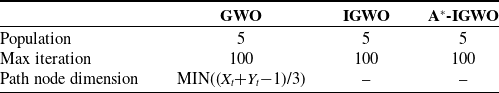
Table I. Parameters of the algorithm.
3.3. A*-IGWO
3.3.1. Theory
A* algorithm use best first search and find the minimum cost path from a given initial node to a target node (from one or more possible targets). When A* algorithm traverses the graph, it follows the path with the lowest known heuristic cost and maintains a ranking priority queue of alternating path segments during this process. Similar to greedy best first search, but more accurate because A* algorithm considers nodes that have already been traversed. A* algorithm represents the minimum cost path to the node, making it the best first search algorithm, as Eq. (14):
 \begin{equation} f\!\left(x\right)=g\!\left(x\right)+h\!\left(x\right) \end{equation}
where g(x) is the total distance from the initial position to the current position, h(x) is a heuristic function used to approximate the distance from the current position to the target state, and f(x) is the current approximation of the shortest path to the target.

Figure 11. The simulation results of IGWO path planner in Test Map 1 #∼Test Map 4 #.
3.3.2. Fitness function of A*-IGWO
In fitness function program STEP 2, the IGWO algorithm filters out the fitness function values of each wolf by determining their size as alpha wolf, beta wolf, and delta wolf. In path planning problems, the fitness function of GWO algorithms is path length. The essence of path planning problem is to find the shortest and unobstructed path between the starting and ending points. In the absence of obstacles, the straight-line distance between two points is the shortest, providing direction for optimizing path length. The closer the path is to the line connecting the starting and ending points, the shorter the distance. The fitness function of GWO algorithms does not reflect this concept, which leads to divergent optimization directions, increases the number of iterations, and makes it easier to fall into local optima.
The fitness function that integrates the minimum cost of the A* algorithm is shown in Eqs. (15) and (16). On the basis of the original path length, the heuristic function g(x) and greedy function h(x) for each path node are added to further constrain the direction of path optimization:
 \begin{equation} \textit{Fitnes}s_{1}=AC_{1}\times \sum \sqrt{\left(x_{i}-x_{i-1}\right)^{2}+\left(y_{i}-y_{i-1}\right)^{2}}+AC_{2}\times \sum \sqrt{\left(x_{e}-x_{i}\right)^{2}+\left(y_{e}-y_{i}\right)^{2}} \end{equation}
 \begin{align} \textit{Fitnes}s_{2}=AC_{1}&\times \sum \sqrt{\left(x_{i}-x_{i-1}\right)^{2}+\left(y_{i}-y_{i-1}\right)^{2}}\nonumber \\[5pt] & + AC_{2} \times \left(\sum \sqrt{\left(x_{e}-x_{i}\right)^{2}+\left(y_{e}-y_{i}\right)^{2}}+\sum \sqrt{\left(x_{i}-x_{s}\right)^{2}+\left(y_{i}-y_{s}\right)^{2}}\right) \end{align}
where AC 1 and AC 2 are coefficients, I is the number of path nodes, xi is the horizontal coordinate of the i-th path node, yi is the i-th coordinate of the path node, xe is the horizontal coordinate of the target position, ye is the vertical coordinate of the target position, xs is the horizontal coordinate of the starting point, and ys is the starting point ordinate.
4. Experimental results and comparison
This section will introduce the following content: (1) path planning simulation of IGWO path planner with improved fitness function and improved position iteration equation; (2) simulation of path planning for IGWO path planners with different convergence factor functions and optimization of convergence factor functions; (3) A*-IGWO path planner simulation for Fitness 1 and Fitness 2 functions; (4) the impact of changes in the coefficients AC 1 and AC 2 of Fitness 1 and Fitness 2 functions on the path planning simulation of A*-IGWO path planner.
Parameter settings for GWO, IGWO, and A*-IGWO path planner: (1) the initial population is 5; (2) the maximum number of iterations is 100; (3) r 1 and r 2 are uniformly distributed random variables on [0,1]; (4) the number of simulations is 20; and (5) the sum of AC 1 and AC 2 is 1.
Table II. The path length of IGWO path planner in Test Map 1 #∼Test Map 4 #.

Table III. The iterations of IGWO path planner in Test Map 1 #∼Test Map 4 #.

The parameters of GWO, IGWO, and A*-IGWO are shown in Table I. Where Xt is the position of target in X-axis and Yt is the position of target in Y-axis.

Figure 12. The simulations of IGWO path planner in 1 # Parking lot ∼ 4 # Parking lot.
4.1. IGWO path planner
4.1.1. Fitness function and position iteration
The simulation results of IGWO path planner using improved fitness function and improved position iteration equation in Test Map 1 #∼Test Map 4 # are shown in Fig. 11, and the simulation results are shown in Tables II and III.
Table IV. The path length of IGWO path planner in 1 # Parking lot ∼ 4 # Parking lot.

Compare with GWO path planner:
-
1. The simulation results in Test Map 1 # show that the average number of iterations for IGWO path planner has decreased by 89.36% and 22.2%, respectively; the optimal number of iterations has been reduced by 50%, reducing by 2; the average path length after iteration decreased by 11.56% and 2.69 m; the optimal path length after iteration has been reduced by 11.56% and 2.69 m.
-
2. The simulation results in Test Map 2 # show that the average number of iterations for IGWO path planner has decreased by 91.7% and 16.8; the optimal number of iterations has been reduced by 82% and 9; the average path length after iteration decreased by 4.81% and 1.12 m; the optimal path length after iteration has been reduced by 4.81% and 1.12 m.
Table V. The iterations of IGWO path planner in 1 # Parking lot ∼ 4 # Parking lot.

Table VI. The path length of different convergence factor in 1 # Parking lot ∼ 4 # Parking lot.

Table VII. The iterations of different convergence factor in 1 # Parking lot ∼ 4 # Parking lot.

-
3. The simulation results in Test Map 3 # show that the average number of iterations for IGWO path planner has decreased by 50.36% and 28.2; the optimal number of iterations has been reduced by 43.75% and 7; the average path length after iteration decreased by 10.88% and 2.62 m; the optimal path length after iteration has been reduced by 7.39% and 1.72 m.
-
4. The simulation results in Test Map 4 # show that the average number of iterations of IGWO path planner has increased by 1640%, an increase of 32.8; the optimal number of iterations increased by 250%, an increase of 5; the average path length after iteration decreased by 7.02% and 1.74 m; and the optimal path length after iteration has been reduced by 7.14% and 1.77 m.
The simulation results of IGWO path planner using improved fitness function and improved position iteration in the 1 # Parking lot ∼ 4 # Parking lot are shown in Fig. 12, and the simulation results are shown in Tables IV and V.
Compare with GWO path planner:
-
1. The simulation results on the 1 # Parking lot show that the average iteration number of IGWO path planner has decreased by 33.61% and 8.2; the optimal number of iterations has been reduced by 75.00% and 15; the average path length after iteration has been reduced by 2.44 m; the optimal path length after iteration has been reduced by 1.57 m.
-
2. The simulation results on the 2 # Parking lot show that the average number of iterations of the IGWO path planner has decreased by 22.63% and 3.1; the average path length after iteration has been reduced by 1.59 m; the optimal path length after iteration has been reduced by 1.54 m.
-
3. The simulation results on the 3 # Parking lot show that the average iteration number of IGWO path planner has increased by 120.00%, an increase of 2.4; the optimal number of iterations increased by 50%, increasing by 1; the average path length after iteration has been reduced by 2.54 m; the optimal path length after iteration has been reduced by 2.54 m.
-
4. The simulation results on the 4 # Parking lot show that the average iteration number of IGWO path planner has increased by 149.18%, an increase of 9.1; the optimal number of iterations has been reduced by 20.00%, reducing by 1; the average path length after iteration has been reduced by 2.42 m; the optimal path length after iteration has been reduced by 3.00 m.
In summary, the IGWO path planner, which applied the improved fitness function and improved position iteration, played a positive role in path planning from 1 # Parking lot to 4 # Parking lot, resulting in a reduction in the length of the iterated path.
4.1.2. Convergence factor
The simulation results of IGWO path planners with different convergence factor functions from 1 # Parking lot to 4 # Parking lot are shown in Tables VI and VII, and the comparison of simulation results is shown in Fig. 13. The simulation results show that the IGWO path planner with a 4 function as the convergence factor has the least number of iterations from 1 # Parking lot to 4 # Parking lot.

Figure 13. The simulation results of different convergence factor.
4.2. A*-IGWO path planner
The simulation results of A*-IGWO path planner using Fitness 1 and Fitness 2 functions as fitness functions in 1 # Parking lot to 4 # Parking lot are shown in Figs. 14–16. Figure 14 shows the comparison of the A*-IGWO path planner and IGWO path planner using the Fitness 1 function with AC 1 = 0.5 and AC 2 = 0.5, as well as the comparison of the optimal path length, average path length, and number of iterations between the 1 # Parking lot and 4 # Parking lot iterations. The results show that the optimal path length and average path length of the A*-IGWO path planner with the Fitness 1 function after iteration are shorter than those of the IGWO path planner. The number of iterations of A*-IGWO path planner using the Fitness 1 function is lower than that of IGWO path planner.

Figure 14. The simulation results of A*-IGWO path planner in 1 # Parking lot ∼ 4 # Parking lot.
Figure 15 shows the results of the A*-IGWO path planner using the Fitness1 function to increase AC 2 from 0.1 to 0.9 after iteration in the 1 # Parking lot to 4 # Parking lot. The results show that when AC 1 = 0.5 and AC 2 = 0.5, the average path length and optimal path length after iteration are the shortest. AC1 affects the fitness function with path length as the optimization result. The smaller AC1, the smaller the proportion of path length as the optimization result; AC2 affects the fitness function part of the path node penalty optimization result guided by the target point. The smaller AC2, the easier the optimization result is to fall into local optima.

Figure 15. The results of the A*-IGWO path planner using the Fitness1 function.
Table VIII. The simulation result of A*-IGWO and GWO algorithm.

Table IX. The simulation result of A*-IGWO, PSO, and A* algorithm.

Table X. The simulation result of A*-IGWO, HSGWO, and Weight Grey Wolf Optimizer (WGWO).

Figure 16 shows the results of the A*-IGWO path planner using the Fitness2 function to increase AC 2 from 0.1 to 0.9 after iteration from 1 # Parking lot to 4 # Parking lot. The results show that when AC 1 = 0.8 and AC 2 = 0.2, the average path length and optimal path length after iteration are the shortest.

Figure 16. The results of the A*-IGWO path planner using the Fitness2 function.
Figure 17 shows the comparison of the simulation results of A*-IGWO path planner using Fitness 1 with AC 1 = 0.5 and AC 2 = 0.5 and Fitness 2 functions with with AC 1 = 0.8 and AC 2 = 0.2 as fitness functions in the 1 # Parking lot to 4 # Parking lot. The results show that the A*-IGWO path planner of the Fitness 2 function with a starting end point direction as the penalty function outperforms the A*-IGWO path planner of the Fitness 1 function with an end point direction as the penalty function in terms of both the number of iterations and the length of the path after iteration.

Figure 17. Comparison of the simulation results of A*-IGWO path planner using Fitness1 and Fitness2 functions.
The simulation results of A*-IGWO compared with GWO in 1 # Parking lot ∼ 4 # Parking lot are shown in Table VIII. The simulation results show that compared with the GWO algorithm, the A*-IGWO algorithm improves the iteration speed and reduces the path length, reducing the iteration number by 69.7% and the path length by 6.1%, which partially solves the local optimal problem of the GWO algorithm in path planning.
4.3. Comparison
4.3.1. PSO and A* algorithm
The number of particles for PSO is 20 and max iterations is 100.
A*-IGWO comparison between PSO and A* algorithm in 1 # Parking lot ∼ 4 # Parking lot is shown in Table IX A*-IGWO has fewer iterations and shorter path lengths. The path length by using A*-IGWO is less than using PSO and A* algorithm,and the number of iterations by using A*-IGWO is less than using PSO algorithm.
4.3.2. HSGWO and IGWO
The parameters of the novel hybrid algorithm (HSGWO) [Reference Qu, Gai, Zhang and Zhong32] and the Improved Gray Wolf Optimization algorithm (IGWO) [Reference Su and Yourui41] are the same as those for A*-IGWO.
A* - IGWO comparison between HSGWO and IGWO in 1 # Parking lot ∼ 4 # Parking lot is shown in Table X. The path length and the number of iterations by using A*-IGWO is less than using HSGWO and IGWO algorithm.
5. Conclusion
This article proposes an A*-IGWO path planner that integrates the A* algorithm to solve the path planning problem of mobile charging robots in parking lots. Firstly, improvements and optimizations to the position update function and convergence factor were proposed for the local optimization problem of GWO path planner; then, using the theory of A* algorithm, an improved A*-IGWO path planner for fitness functions was proposed, and the coefficients AC 1 and AC 2 of Fitness 1 and Fitness 2 functions were studied; finally, the path planner was used to simulate and analyze the path planning of four randomly parked parking lot environments. The results indicate that the A*-IGWO path planner outperforms the GWO path planner in terms of iteration and path length and partially solves the local optimization problem of the GWO path planner. Compared with the GWO algorithm, the A*-IGWO algorithm improves the iteration speed and reduces the path length, reducing the iteration number by 69.7% and the path length by 6.1%, which partially solves the local optimal problem of the GWO algorithm in path planning.
Author contribution
In this article, author Shangjunnan Liu completed the parts of model, algorithm, simulation, and analysis; author Shuhai Liu provided technical support and guidance; author Huaping Xiao provided writing guidance.
Financial support
This work is funded and supported by the Beijing Natural Science Foundation under the following project reference: 3232013.
Competing interests
The authors declare no competing interests exist.


