


1. Introduction
The distribution of buoyant material in the ocean, including microplastics, oil droplets, phytoplankton cells, sargassum and debris, has important implications for marine life and safety. Buoyant material is less dense than seawater and, hence, tends to remain close to the surface of the ocean. Buoyant material can accumulate in localised regions due to horizontally convergent surface currents associated with a variety of physical processes (van Sebille et al. Reference van Sebille2020).
Consider as an example the case of microplastics. Larger plastics that are deposited into the ocean as waste are fragmented into microplastics through UV radiation, chemical degradation and mechanical abrasion. Plastic is usually buoyant, with an average material density of 965 kg m $^{-3}$ compared with the average density of surface seawater, 1027 kg m $^{-3}$ (Morét-Ferguson et al. Reference Morét-Ferguson, Law, Proskurowski, Murphy, Peacock and Reddy2010). It is estimated that there are up to 51 trillion pieces of microplastic at the surface of the ocean, corresponding to a mass of up to 236 thousand metric tonnes (van Sebille et al. Reference van Sebille, Wilcox, Lebreton, Maximenko, Hardesty, Van Franeker, Eriksen, Siegel, Galgani and Law2015). Plastics degrade very slowly and can be ingested by marine life, often at the surface of the ocean (Wilcox et al. Reference Wilcox, van Sebille, Hardesty and Estes2015; Compa et al. Reference Compa, Alomar, Wilcox, van Sebille, Lebreton, Hardesty and Deudero2019).
Buoyant material that is small enough to be treated as a point particle (i.e. the shape does not matter) can be referred to as a buoyant particle. When the concentration of buoyant particles is sufficiently low, interactions between particles and their effect on the flow can be neglected. In these cases, the concentration of buoyant particles is often modelled using a continuum approximation. We use the term buoyant tracer to describe such a concentration field, which has previously been used to model microplastics (Kukulka & Brunner Reference Kukulka and Brunner2015), oil droplets (Yang, Chamecki & Meneveau Reference Yang, Chamecki and Meneveau2014) and phytoplankton cells (Smith, Hamlington & Fox-Kemper Reference Smith, Hamlington and Fox-Kemper2016).
Due to their low density, buoyant particles tend to remain in the ocean mixed layer (OML). The OML is the uppermost part of the ocean where turbulence driven by atmospheric forcing maintains weak density stratification. Here, buoyant particles are subject to a variety of processes including convective plumes, Langmuir and wind-driven turbulence, submesoscale eddies, Ekman flow and Stokes drift.
Buoyant particles accumulate due to convergent surface currents on a wide range of scales. On a global scale, convergent wind-driven currents cause microplastics to accumulate in mid-ocean gyres (Cole et al. Reference Cole, Lindeque, Halsband and Galloway2011; Eriksen, Thiel & Lebreton Reference Eriksen, Thiel and Lebreton2017). On the submesoscale (1–10 km), strongly convergent flow causes oil and surface particles to accumulate in narrow (10–100 m) density fronts (D'Asaro et al. Reference D'Asaro2018; Taylor Reference Taylor2018). On smaller scales, wind- and buoyancy-driven turbulence cause buoyant particles to accumulate in ephemeral patches and streaks. Here, our focus is on these small scales that will be reviewed briefly below.
When wind and surface waves align, Langmuir circulation or Langmuir turbulence can arise, consisting of longitudinal circulation cells aligned with the wind and waves (Leibovich Reference Leibovich1983; Thorpe Reference Thorpe2004). These circulation cells are often visible through lines of buoyant material that accumulate in regions of surface convergence (Langmuir Reference Langmuir1938). Skyllingstad & Denbo (Reference Skyllingstad and Denbo1995) used numerical simulations to study the horizontal distribution of surface particles under a Langmuir turbulent regime and they, alongside a number of other studies (McWilliams, Sullivan & Moeng Reference McWilliams, Sullivan and Moeng1997; McWilliams & Sullivan Reference McWilliams and Sullivan2000), observed surface particles accumulating in narrow downwelling streaks. Yang et al. (Reference Yang, Chamecki and Meneveau2014) expanded on this by investigating a buoyant tracer with a wide range of buoyancies under Langmuir turbulence. They found that the degree of particle accumulation in the windrows was impacted by the tracer buoyancy, with the more buoyant tracer being more clustered. Kukulka & Brunner (Reference Kukulka and Brunner2015) and Brunner et al. (Reference Brunner, Kukulka, Proskurowski and Law2015) used numerical simulations and analytical models to show that Langmuir turbulence is not only important in determining the horizontal distribution, but also in vertically transporting buoyant particles deep into the OML.
In the absence of Stokes drift, the small-scale structure of the OML is often governed by processes such as convection forced from night-time cooling and shear stress generated by surface winds. Kukulka, Law & Proskurowski (Reference Kukulka, Law and Proskurowski2016) used observations and numerical simulations to show that turbulence generated by convection can deeply submerge buoyant particles, whilst Kukulka et al. (Reference Kukulka, Proskurowski, Morét-Ferguson, Meyer and Law2012) used observations and a one-dimensional column model to study wind-driven vertical mixing of plastic debris. Skyllingstad & Denbo (Reference Skyllingstad and Denbo1995) showed that under a combination of wind and convective forcing, the horizontal distribution of particles at the ocean surface coincides with regions of convergence. Mensa et al. (Reference Mensa, Özgökmen, Poje and Imberger2015) used a relatively low-resolution model to demonstrate that under pure convection, tracer accumulates in convergent regions of Rayleigh–Bénard cells. With the additional presence of weak wind forcing, they found that convection cells were distorted but tracer continued to accumulate in downwelling regions. Chor et al. (Reference Chor, Yang, Meneveau and Chamecki2018a) expanded on this using higher resolution numerical simulations in a purely convective regime and a range of buoyancies for the tracer field. They found that, in addition to buoyant particles accumulating in convergent regions of the Rayleigh–Bénard cells, the presence of convective vortices in the vertices between some cells acted to additionally cluster the most buoyant particles. It remains unclear to what extent convective vortices and the associated accumulation of buoyant particles persist in the presence of wind forcing.
Here, we extend previous work by studying the formation and persistence of convective vortices under the combined effects of wind and convective forcing and their influence on buoyant material. In the atmosphere it has been noted that the number and strength of convective vortices (e.g. dust devils) that form depend strongly on wind conditions (Raasch & Franke Reference Raasch and Franke2011). In the context of the ocean, Heitmann & Backhaus (Reference Heitmann and Backhaus2005) found that there is a transition from convective cells to longitudinal wind rolls as wind forcing is added to convection, with three distinct flow patterns being observed under weak, moderate and strong wind forcing.
We study these processes using a series of large eddy simulations (LES) under idealised conditions where turbulence is generated by imposing a constant surface heat flux and shear stress. Large eddy simulation is a useful tool for studying the accumulation of buoyant particles because they resolve the largest turbulent motions responsible for particle accumulation and vertical transport. Large eddy simulation has also been used to study convective vortices in the atmosphere (Raasch & Franke Reference Raasch and Franke2011) and the ocean (Chor et al. Reference Chor, Yang, Meneveau and Chamecki2018a).
We model buoyant material using a combination of tracers and Lagrangian particles advected with the surface velocity (also commonly known as surface drifters). The concentration of buoyant particles can be represented with a tracer field with additional advection by a slip velocity that depends on the modelled particle size and density. The upwards slip velocity causes buoyant tracers to concentrate near the surface of the ocean and is opposed by turbulence and diffusion that transports the tracer downwards. For a buoyant tracer to be effectively trapped at the surface, the slip velocity must exceed the maximum vertical velocity of the fluid. Due to numerical constraints, there is a limit to the slip velocity that can be added to a tracer field. Here, we additionally use Lagrangian particles at the surface that allows us to investigate the limit where the slip velocity is much larger than the fluid vertical velocity.
Whilst Chor et al. (Reference Chor, Yang, Meneveau and Chamecki2018a) provides an extensive study of convective vortices in a purely convective regime, we focus on the extent to which convective vortices persist in the presence of a surface wind stress, and how this affects particle clustering inside convective vortices. Unlike our simulations, Chor et al. (Reference Chor, Yang, Meneveau and Chamecki2018a) did not include the Coriolis acceleration due to the Earth's rotation and, hence, they did not observe the bias towards cyclonic convective vortices that we observe. Additionally, Chor et al. (Reference Chor, Yang, Meneveau and Chamecki2018a) only used a tracer field to investigate clustering of buoyant material and did not look at the limit of extremely buoyant material with Lagrangian particles.
Below, in § 2, we introduce the problem configuration and numerical methods. In § 3 we present our results. Section 3.1 includes a qualitative description of the flow and the buoyant particles, § 3.2 describes convective vortices with and without wind forcing, and § 3.3 includes a quantification of the accumulation of buoyant particles. A summary of the study and discussion of the key results is given in § 4.
2. Set-up and numerical methods
Here, we use LES to solve a low-pass filtered version of the non-hydrostatic incompressible Boussinesq Navier–Stokes equations (2.1) and (2.2) in terms of the low-pass filtered velocity  ${\boldsymbol u}=(u,v,w)$, low-pass filtered pressure $p$ and buoyancy $b$,
$b$,
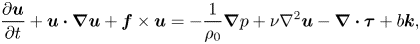 $$\begin{gather} \frac{\partial {\boldsymbol u}}{\partial t}+{{\boldsymbol u}} \boldsymbol{\cdot} \boldsymbol{\nabla} {\boldsymbol u} + {\boldsymbol f} \times {\boldsymbol u} ={-} \frac{1}{\rho_0} \boldsymbol{\nabla} p + \nu \nabla^2 {\boldsymbol u} - \boldsymbol{\nabla} \boldsymbol{\cdot} {\boldsymbol \tau} + b {\boldsymbol k}, \end{gather}$$
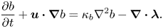 $$\begin{gather}\frac{\partial b}{\partial t}+{\boldsymbol u}\boldsymbol{\cdot} \boldsymbol{\nabla} b = \kappa_b \nabla^2 b - \boldsymbol{\nabla} \boldsymbol{\cdot} {\boldsymbol \lambda}. \end{gather}$$
The buoyancy is treated as a single scalar variable under the assumption of a linear equation of state and neglecting double diffusive effects. In the momentum equation (2.1),  ${\boldsymbol f}=(0,0,f)$ is the Coriolis parameter, $\rho _0$ is the reference density, ${\boldsymbol k}$ is the unit vector in the vertical direction and ${\boldsymbol \tau }$ is the subgrid scale stress tensor. In the buoyancy equation (2.2), ${\boldsymbol \lambda }$ is the subgrid scale scalar flux. Both ${\boldsymbol \tau }$ and ${\boldsymbol \lambda }$ are calculated using the anisotropic minimum dissipation model (Abkar, Bae & Moin Reference Abkar, Bae and Moin2016; Vreugdenhil & Taylor Reference Vreugdenhil and Taylor2018), which is described below.
The computational domain is 500 m in each horizontal direction and 120 m in the vertical direction. A constant buoyancy loss (equivalent to cooling the surface of the ocean) is applied at the surface to drive convection. Various values of the imposed surface buoyancy flux are used, ranging from 0 to  $-4.24 \times 10^{-8}$ m $^2$ s $^{-3}$, but the surface buoyancy flux is constant in each simulation. Using a thermal expansion coefficient of $\alpha = 1.65 \times 10^{-4}\, {}^{\circ}$C $^{-1}$ and a heat capacity of $4 \times 10^{-3}$ J kg ${}^{\circ}$C $^{-1}$, a surface buoyancy flux of $-4.24\times 10^{-8}$ m $^2$ s $^{-3}$ corresponds to a heat loss of about 100 Wm $^{-2}$. Wind is applied using a shear stress at $z=0$ that is aligned with the $x$ axis without loss of generality. Various values of the wind stress are considered, ranging from 0 to 0.1 Nm $^{-2}$, but again this value is constant for each simulation. At the bottom of the computational domain, a no stress boundary condition is applied in both horizontal directions and a sponge layer is applied to prevent reflections. Planetary rotation is included with a Coriolis parameter of $f=10^{-4}$ s $^{-1}$. At $t=0$, the buoyancy is initialised with a mixed layer with depth 80 m overlying a region with stable stratification. Specifically, $\partial b/\partial z =0$ s $^{-2}$ for $-80$ m $< z<0$ and $\partial b/\partial z=9\times 10^{-6}$ s $^{-2}$ for $z<-80$ m. This stratification is in the range of values observed by Brainerd & Gregg (Reference Brainerd and Gregg1993) in the diurnal thermocline and is equivalent to a potential temperature gradient of $\partial \theta /\partial z= 0.01\,^\circ$C m $^{-1}$ for $z<-80$ m.
The vertical velocity is set to zero at the top and bottom of the domain. We also do not include the Craik–Leibovich vortex force, and hence, we neglect the influence of surface waves and Langmuir circulation. Hence, although we run simulations for about 24 hours to allow wind and convective turbulence to fully develop, we do not consider the development of surface waves or Langmuir circulation. This can be viewed as an approximation to calm conditions (e.g. at the start of a wind event before waves have had time develop), but our primary motivation is to simplify the physical processes and isolate the influence of wind-driven shear on convective vortices. Periodic boundary conditions are applied in both horizontal directions. The velocity is initialised as random white noise with an amplitude of  $10^{-4}$ m s $^{-1}$. The molecular viscosity is $\nu = 10^{-6}$ m $^2$ s $^{-1}$ and the molecular diffusivity is $\kappa _b = 10^{-6}$ m $^2$ s $^{-1}$, although both are small compared with the subgrid scale terms and do not directly influence the model results.
The resolved fields are discretised on a grid with 512 points in each horizontal direction and 65 points in the vertical direction. This gives a horizontal grid spacing of 0.98 m and a variable vertical grid spacing between 0.95 m and 2.57 m with higher resolution near  $z=0$. Derivatives in the horizontal directions are calculated using a pseudospectral method, whilst vertical derivatives are approximated using second-order finite differences. The equations are time stepped using an implicit Crank–Nicolson method for the viscous and diffusive terms and a third-order Runge–Kutta method for all other terms. Further details of the numerics can be found in Taylor (Reference Taylor2008).
The subgrid scale terms are modelled with the anisotropic minimum dissipation (AMD) model (Rozema et al. Reference Rozema, Bae, Moin and Verstappen2015; Abkar et al. Reference Abkar, Bae and Moin2016; Vreugdenhil & Taylor Reference Vreugdenhil and Taylor2018). In developing our simulations, we also tested the constant Smagorinsky model but found that the AMD model converged more rapidly as the resolution was increased. With the AMD model, the dynamics under pure convection are relatively insensitive to grid spacing. In the wind-forced case, the root-mean-square (r.m.s.) vertical velocity and pressure near the surface increase as the resolution increases. This is likely due to an additional small-scale turbulence near  $z=0$ being resolved in higher resolution runs. However, at a depth of $-$30 m, close to the depth where the r.m.s. vertical velocity reaches its maximum, the vertical velocity is only weakly dependent on the resolution under both convection and wind forcing. A detailed discussion of the resolution convergence can be found in the appendix.
Buoyant material is modelled using two approaches: an Eulerian tracer concentration field and Lagrangian surface particles. The set-up for the Eulerian tracer concentration field is similar to Taylor (Reference Taylor2018) and Chor et al. (Reference Chor, Yang, Meneveau and Chamecki2018a). The tracer is modelled as a continuous concentration of non-interacting particles. Each particle moves with the local fluid velocity plus a constant upwards slip velocity. This is equivalent to considering small, buoyant particles of a fixed size and density. We assume low tracer concentrations, so although the tracers themselves are buoyant, they do not affect fluid buoyancy. The equation for the concentration of buoyant material is given by
 \begin{equation} \frac{\partial c}{\partial t} + {\boldsymbol u} \boldsymbol{\cdot} \boldsymbol{\nabla} c + w_s \frac{\partial c}{\partial z}= \boldsymbol{\nabla} \boldsymbol{\cdot} ((\kappa_{SGS}+\kappa_c) \boldsymbol{\nabla} c), \end{equation}
where  $w_s$ is the constant slip velocity and $\kappa _{SGS}$ is the subgrid scale diffusivity. We set $\kappa _c=\kappa _b=10^{-6}~\mbox {m}^2~\mbox {s}^{-1}$, although this value is very small compared with $\kappa _{SGS}$ and does not influence the tracer concentration. The buoyant tracer concentration is updated using the same numerical method as the main LES code. A small number of negative values of the tracer concentration occur due to Gibbs ringing at the grid scale, but the total tracer concentration is conserved by the numerical scheme. The initial condition of the tracer is exponential in depth, specifically $c(x,y,z,t=0)={\rm e}^{z/10\ \mbox {m}}$. In this study, three tracers are considered with slip velocities of $w_s= 0.001$, 0.005, 0.01 m s $^{-1}$. Experiments on a sample of microplastics from the North Atlantic subtropical gyre estimate the slip velocity to be between 0.005 and 0.025 m s $^{-1}$ (Kooi et al. Reference Kooi2016), which coincides with the two most buoyant tracers in our simulations. Above a value of 0.01 m s $^{-1}$ the continuous tracer field exhibits significant numerical noise that prevents us from further increasing the slip velocity.
To investigate buoyant material with higher slip velocities, we turn to Lagrangian particles. The particles are one way coupled; they do not affect the surrounding flow. We also neglect interactions between particles. The movement of small inertial spherical particles is described by the Maxey–Riley equation (Maxey & Riley Reference Maxey and Riley1983). We begin with a simplified version of the full equation which is the starting point for most studies of inertial particles in turbulent flows (Balkovsky, Falkovich & Fouxon Reference Balkovsky, Falkovich and Fouxon2001; Chamecki et al. Reference Chamecki, Chor, Yang and Meneveau2019). In this equation, the Faxen correction, Basset history force and lift force are neglected on the basis that the radius of the particle is much smaller than the scales over which the fluid velocity changes. Brownian motion is neglected on the basis that molecular viscosity is very small ( $\nu =10^{-6}$ m $^2$ s $^{-1}$ in our simulations), but some random motion is accounted for in a subgrid scale model discussed below. Under these assumptions, the particle velocity, ${{\boldsymbol v}}_p$, satisfies the equation
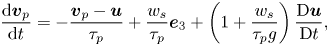 \begin{equation} \frac{\mathrm{d} {\boldsymbol v}_p}{\mathrm{d} t}={-}\frac{{\boldsymbol v}_p-{\boldsymbol u}}{\tau_p}+ \frac{w_s}{\tau_p}{{\boldsymbol e}}_3+\left(1+\frac{w_s}{\tau_p g}\right)\frac{\mathrm{D}{\boldsymbol u}}{\mathrm{D}t},\end{equation}
where  ${{\boldsymbol u}}$ is the fluid velocity, $\tau _p$ is the particle response time and $w_s$ is the terminal slip velocity. When $Re_p \ll 1$ (where $Re_p=|{{\boldsymbol v}}_p - {{\boldsymbol u}}|d_p/\nu$ is the particle Reynolds number), particles are described as being in the Stokes regime and the particle response time and terminal slip velocity are defined as
 $$\begin{gather} \tau_p = \frac{(\rho_p + \rho_f/2)d_p^2}{18 \mu_f}, \end{gather}$$
 $$\begin{gather}w_s=\frac{(\rho_p-\rho_f)gd_p^2}{18\mu_f}, \end{gather}$$
where the terminal slip velocity is a balance between the Stokes drag and buoyancy force only. Here,  $\rho _p$ is the particle density, $d_p$ is the particle diameter, $\rho _f$ is the fluid density and $\mu _f$ is the dynamic viscosity of the fluid.
Further simplifications of (2.4) can be made by looking at the Stokes number that characterises the tendency of a particle to move with the fluid velocity. The Stokes number is defined as the ratio between the particle response time and the turbulence time scale,  $St=\tau _p/\tau _t$. A very small Stokes number indicates that the particle motion is strongly influenced by the fluid flow whilst a large Stokes number indicates that the particle moves independently of the fluid. The Stokes number for microplastics has been estimated to be between ${O} (10^{-3})$ and ${O} (10^{-2})$ at the surface (Kukulka et al. Reference Kukulka, Proskurowski, Morét-Ferguson, Meyer and Law2012; Chamecki et al. Reference Chamecki, Chor, Yang and Meneveau2019), which corresponds to microplastics of about 1 cm or less (Poulain et al. Reference Poulain, Mercier, Brach, Martignac, Routaboul, Perez, Desjean and Ter Halle2018). In the limit where $St \ll 1$, (2.4) can be approximated as (Ferry & Balachandar Reference Ferry and Balachandar2001; Yang et al. Reference Yang, Chen, Socolofsky, Chamecki and Meneveau2016)
 \begin{equation} {{\boldsymbol v}}_p={{\boldsymbol u}} + w_s {{\boldsymbol e}}_3 + \frac{w_s}{g} \frac{\mathrm{D}{\boldsymbol u}}{\mathrm{D}t}. \end{equation}
The last term on the right-hand side is the leading-order inertial effect and, similarly to Chor et al. (Reference Chor, Yang, Meneveau and Chamecki2018a), we are interested in flows for which  $g^{-1} \mathrm {D}{{\boldsymbol u}}/\mathrm {D}t \ll 1$. This reduces our particle motion equation to
 \begin{equation} {{\boldsymbol v}}_p={{\boldsymbol u}} + w_s {{\boldsymbol e}}_3. \end{equation}
This describes particles for which inertial effects are negligible compared with flow advection and buoyancy effects. In this study we use the Lagrangian approach to investigate the limit of extremely buoyant particles and implement a two-dimensional (2-D) particle model at the surface of the domain, which can be interpreted as the limit where  $w_s \gg |w|$. To model the influence of unresolved turbulence on particle motion, a random displacement is included following the approach in Liang et al. (Reference Liang, Wan, Rose, Sullivan and McWilliams2018). This gives the equations for the motion of 2-D non-inertial particles as
 $$\begin{gather} {\boldsymbol x}_p (t+{\rm d}t) = {\boldsymbol x}_p(t) + {\boldsymbol u}({\boldsymbol x}_p,t)\, {\rm d} t + {\boldsymbol x}_{sgs}({\boldsymbol x}_p,t), \end{gather}$$
 $$\begin{gather}{\boldsymbol x}_{sgs,i}=\frac{\partial \nu_{sgs}}{\partial x_i} ( {\boldsymbol x}_p,t)\, {\rm d}t +(2 (\nu_{sgs}({\boldsymbol x}_p,t))_+)^{{1}/{2}} \,{\rm d} \xi _i. \end{gather}$$
In (2.9),  ${\boldsymbol u}$ is the resolved velocity interpolated at the particle position and ${\boldsymbol x}_{sgs}$ is the displacement due to subgrid scale motion. In (2.10) the subscript $i$ indicates the spatial dimension, $\nu _{sgs}$ is the subgrid scale viscosity interpolated at the particle position, ${\rm d} \xi _i$ is Gaussian white noise with variance ${\rm d}t$ and $(\cdot)_+ = max(\cdot ,0)$.
Interpolated quantities are calculated using cubic B splines following van Hinsberg et al. (Reference van Hinsberg, ten Thije Boonkkamp, Tosch and Clercx2012). This method was chosen due to its low computational cost and high accuracy. The particle evolution equations are time stepped using the third-order Runge–Kutta method alongside the main LES code. We simulate the motion of 4000 particles that are initially randomly distributed. In the appendix we discuss the sensitivity of particle clustering to the resolution of the LES and find that in the cases with pure convective forcing, the results are not very sensitive to resolution. In the wind-forced case increasing the resolution slightly reduces the tendency for the particles to cluster.
Here, we report seven simulations with different values of the surface buoyancy flux and wind stress. The parameter space can be interpreted in terms of the friction velocity  $u^*$ and the convective velocity $w^*$ (Deardorff Reference Deardorff1970) that characterise the velocity scales of wind-driven turbulence and convection, respectively. These are defined as
 $$\begin{gather} u^*= \left(\frac{\tau}{\rho_0}\right)^{{1}/{2}}, \end{gather}$$
 $$\begin{gather}w^*=(B_0 h)^{{1}/{3}}. \end{gather}$$
Here,  $\tau$ is the surface wind stress, $\rho _0$ is the constant reference seawater density, $B_0$ is the surface buoyancy flux and $h$ is the initial mixed layer depth. The ratio between $u^*$ and $w^*$ measures the relative importance of wind and convection.
There is some disagreement in the literature as to the ratio of  $u^*$ and $w^*$ that marks a transition from convective turbulence to stress-driven turbulence. For example, early numerical studies using LES estimated that a value of $u^*/w^*=0.65$ marks the change from convective cells to convective rolls in the atmospheric boundary layer (Moeng & Sullivan Reference Moeng and Sullivan1994), whilst for convection between flat plates, the estimated transitional value is $u^*/w^*=0.35$ (Sykes & Henn Reference Sykes and Henn1989). In the ocean, Heitmann & Backhaus (Reference Heitmann and Backhaus2005) found a change in flow behaviour for $u^*/w^*=0.4-0.7$. Regardless of the transition value, we expect wind-driven turbulence to dominate when $u^*/w^* \gg 1$ and convection to dominate when $u^*/w^* \ll 1$. For intermediate values, both wind and convective forcing likely both influence the dynamics to some degree. In the context of vertical mixing of buoyant materials, Chor et al. (Reference Chor, Yang, Meneveau and Chamecki2018b) introduced a generalized turbulence velocity scale, $W$, and in the absence of Langmuir turbulence this is given by
 \begin{equation} W^3=u^{*3}\kappa^3 + A_c^3 w^{*3},\end{equation}
where  $\kappa =0.41$ is the von Kármán constant and $A_c$ represents the contribution of convective turbulence to $W$ that Chor et al. (Reference Chor, Yang, Meneveau and Chamecki2018b) estimated to be $A_c=1.170$. The larger convective coefficient suggests that vertical mixing is influenced more strongly by convective turbulence than wind shear when $u^*=w^*$. The Monin–Obukhov length scale also characterises the importance of convective forcing and wind forcing, and is defined as
 \begin{equation} L=\frac{-u^{*3}}{\kappa B_0}, \end{equation}
where  $\kappa$ is the von Kármán constant as above and $B_0$ is the surface buoyancy flux. In case II defined below ( $u^*=w^*$), we find that $L=58$ m, which predicts that wind forcing is important throughout the upper part of the mixed layer.
Our simulations can be arranged into two series, each independently varying the strength of the wind or the convective forcing. This includes one simulation with pure convection and one simulation with pure wind forcing, which act as control simulations. The first series is run with a surface buoyancy flux held constant at  $-4.24\times 10^{-8}$ m $^2$ s $^{-3}$ and the wind stress varying between $0$ and $0.1$ Nm $^{-2}$, which is equivalent to wind velocities at $10$ m ranging between $0$ and $8.1$ m s $^{-1}$ (calculated using a drag coefficient $C_D=0.0013$). The second series is run with wind stress held constant at 0.1 Nm $^{-2}$ and the surface buoyancy flux varying between 0 and $-4.24\times 10^{-8}$ m $^2$ s $^{-3}$. This allows us to see the effect of increasing wind and convection independently and ensures that we cover a wide range of flow behaviour without applying unrealistic wind or convection forcing. Each simulation has a different value of $u^*/w^*$. The parameters of the simulations are listed in table 1, and the parameter space can be visualised in figure 1.
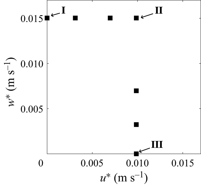
Figure 1. The  $u^*$ and $w^*$ parameter space for simulations. Cases I, II and III are labelled for reference.
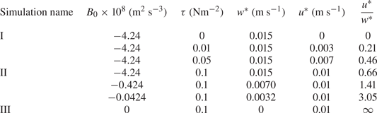
Table 1. Simulation parameters.
3. Results
Here, we primarily focus on three simulations that illustrate the three main flow regimes: pure convection (case I), combined wind and convection (case II) and pure wind forcing (case III). In case I,  $w^*=0.01$ m s $^{-1}$ and $u^*=0$; in case II, $w^*=u^*=0.01$ m s $^{-1}$; and in case III, $w^*=0$ and $u=0.01$ m s $^{-1}$. This allows us to directly examine convection and wind forcing of similar strengths. The remaining simulations exhibit qualitative features that are represented in one of these three cases. In all analyses below, we neglect transient effects by considering horizontal slices at $t = 12$ hours and calculate time averages over one inertial period from $6\unicode{x2013}23.5$ hours. This ensures that the simulated flow has reached a fully developed turbulent condition before the start of the time average. In cases I and II, quasi-steady convection is established by approximately 4 hours. This suggests that our results might be consistent with at least part of the diurnal cycle when night-time convection becomes fully developed.
The results are organised into three subsections: in § 3.1 we present a qualitative description of the flow, buoyant tracers and surface particles; in § 3.2 we investigate the formation of convective vortices and the influence of wind forcing on the vortices; in § 3.3 we look at the accumulation of the buoyant tracer and surface particles.
3.1. Qualitative description of the flow and the distribution of buoyant material
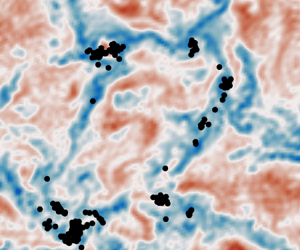
In this section we start by describing the qualitative features of the turbulence and the distribution of buoyant tracers and particles in cases I, II and III. Figure 2 shows horizontal slices of the vertical velocity, tracer concentration and surface particle positions. The vertical velocity field is shown 5 m below the surface. The tracer concentration and particles are shown at the surface ( $z=0$). We show the tracer with $w_s=0.005$ m s $^{-1}$, which is the intermediate buoyancy used in our simulations. A smaller value of $w_s$ gives a more uniformly distributed tracer field, whilst a larger value of $w_s$ gives a more strongly clustered tracer field (shown below). In all of the cases, the average vertical fluid velocity is zero due to the boundary conditions at the surface. The regions of downwelling appear to occupy a smaller area (particularly in cases I and II) but are larger in magnitude.
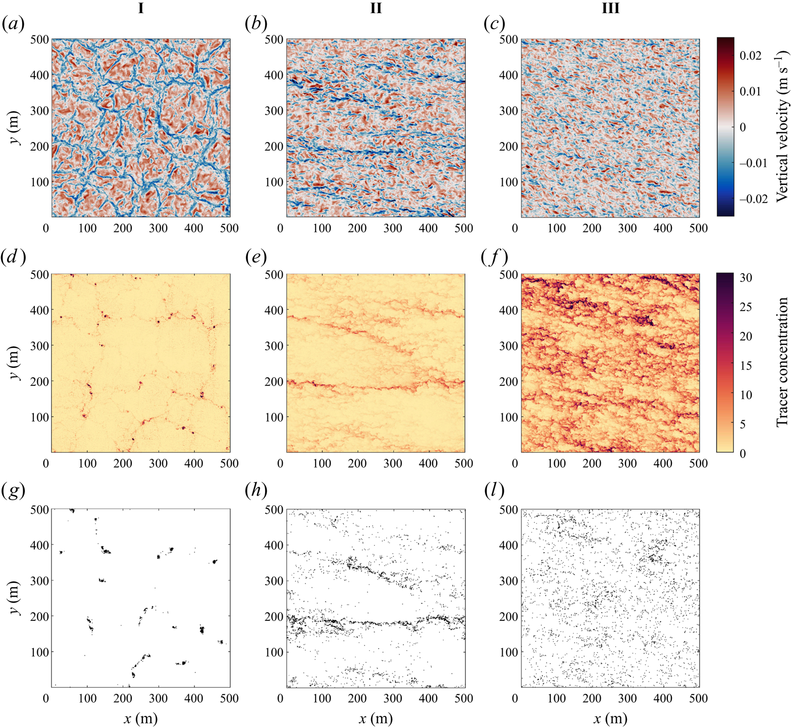
Figure 2. Horizontal cross-sections of the vertical velocity at  $z=-5$ m (a)–(c), tracer concentration with slip velocity 0.005 m s $^{-1}$ at $z=0$ (d)–( f) and particle position at $z=0$ (h)–(j).
In case I distinct convection cells are visible. Convective cells are characterised by large areas of weak upwelling surrounded by narrow regions of strong downwelling. The downwelling regions between neighbouring convective cells meet at convective ‘nodes’. As in Chor et al. (Reference Chor, Yang, Meneveau and Chamecki2018a), the horizontal scale of the convective cells is typically about 1–2 times the depth of the mixed layer (recall that the mixed layer depth is 80 m). The buoyant tracer concentration is elevated in locations of downwelling between convective cells with the highest concentrations in the nodes. The particles, which unlike the tracer are confined to the surface, have a more extreme distribution and are located almost exclusively in the nodes.
In case II with convective and wind forcing, the convection cells are replaced by distinct larger-scale downwelling streaks. The tracer accumulates in the streaks with the strongest downwelling. This is mirrored in the distribution of surface particles. In case III with pure wind forcing, the vertical velocity exhibits horizontal streaks on a smaller scale compared with case II and the tracer concentration also exhibits streaks. In § 3.3 we show that the tracer accumulates in streaks of high speed. The average tracer concentration is noticeably higher at the surface for the same buoyancy (discussed below). The surface particles appear to be less organised than the tracer in this case, although this might be due to the small size of the wind-driven turbulent streaks and the limited number of particles. Inherent differences between Eulerian and Lagrangian dynamics and statistics is interesting, but we are not able to comment on this directly since the tracers and particles sample different depths in our simulations. Still, some areas exhibit elevated particle concentrations and the particles are not uniformly distributed.
As the slip velocity of the tracer increases, the surface tracer concentration increases and the tracer becomes more clustered. Figure 3 shows the tracer distribution at the surface with increasing slip velocity (left to right) in case II. The least buoyant tracer concentration (left) exhibits horizontal streaks but with smaller variations (note the difference in colour axis scale for the three horizontal slices). The most buoyant tracer (right) is more strongly clustered; it has wide expanses of low concentration as well as a few large-scale horizontal streaks with a very high tracer concentration, up to 50 times higher than the least buoyant tracer. The distribution of surface particles (see figure 2i) exhibits the same patterns as the most buoyant tracer. Note that the mean surface tracer concentration is also significantly higher for the more buoyant tracers, and this is discussed further below.
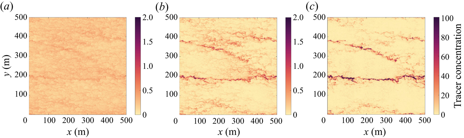
Figure 3. Horizontal cross-section at  $z=0$ of the tracer with $w_s=0.001$ m s $^{-1}$ (a), $w_s=0.005$ m s $^{-1}$ (b), $w_s=0.01$ m s $^{-1}$ (c) in case II.
The influence of the slip velocity on the tracer distribution can be explained in terms of the ability of the vertical fluid velocity to overcome the slip velocity. For all three tracers, the slip velocity is smaller than the maximum vertical velocity (approximately 0.02 m s $^{-1}$). Tracer accumulates in regions of horizontal flow convergence, and at the surface this coincides with downwelling regions of the flow where tracer can be transported below the surface. A less buoyant tracer is more easily submerged and may then resurface in an upwelling (horizontally divergent) region giving a more uniform distribution. Very buoyant tracers are only subducted in regions of strong downwelling and the tracer then quickly rises back to the surface. As a result, very buoyant tracers remain close to regions of strong horizontal convergence and downwelling. It is worth noting, however, that not all downwelling regions exhibit high tracer concentrations. In case I the buoyant tracer and surface particles are strongly clustered in a subset of the convective nodes. As we will see in the next section, these regions are occupied by convective vortices.
Figure 4 shows vertical profiles of the mean tracer concentration (horizontally and time averaged) under different wind and convection forcing conditions. In all cases, the mean tracer concentration is surface intensified and the concentration at  $z=0$ is highest for the most buoyant tracer. As noted from visualisations of the buoyant tracer (figure 2), the mean tracer concentration is noticeably higher at the surface in case III compared with cases I and II. This is confirmed in figure 4, which shows that in case III the vertical distribution of the mean tracer concentration is significantly different from cases I and II. For all slip velocities in case III, the tracer concentration at the bottom of the mixed layer ( $z=-80$ m) is small compared with the surface concentration ( $z=0$). In comparison, the mean tracer concentration profiles in cases I and II are quite similar. In both cases the weakly buoyant tracers are relatively homogeneous in the middle of the mixed layer (i.e. $-60\ \mbox {m}< z<-20$ m). These vertical profiles closely resemble those in Chor et al. (Reference Chor, Yang, Meneveau and Chamecki2018b) and suggest that vertical mixing by convection is fast enough to overcome the effects of tracer buoyancy with or without wind forcing. The turbulence velocity scale, $W$ (see (2.13)), predicts that convective forcing contributes to vertical mixing more than wind shear when $u^*= w^*$, and explains why the vertical distribution of the buoyant tracers in case II is more similar to case I than case III.
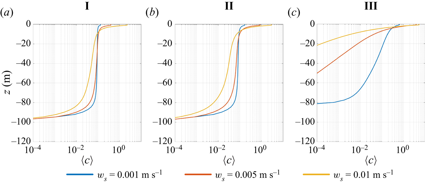
Figure 4. Vertical profile of mean tracer concentrations.
Although the mean tracer concentration is relatively constant in the vertical direction in cases I and II, the tracer concentration within the mixed layer is not uniform. Figure 5 shows the tracer concentration on horizontal slices at  $z=-30$ m. By comparing with figure 2, it is evident that regions with high tracer concentration at $z=-30$ m generally coincide with regions with high concentration at $z=0$. This suggests that regions with elevated tracer concentration are vertically coherent in cases I and II. There are also small areas of very high concentration, particularly visible in case I. These are generally co-located with the surface particles and in the next section we will show that these correspond to convective vortices. In case III there are a few small spots with an elevated tracer concentration, but the concentration is generally quite small at this depth.
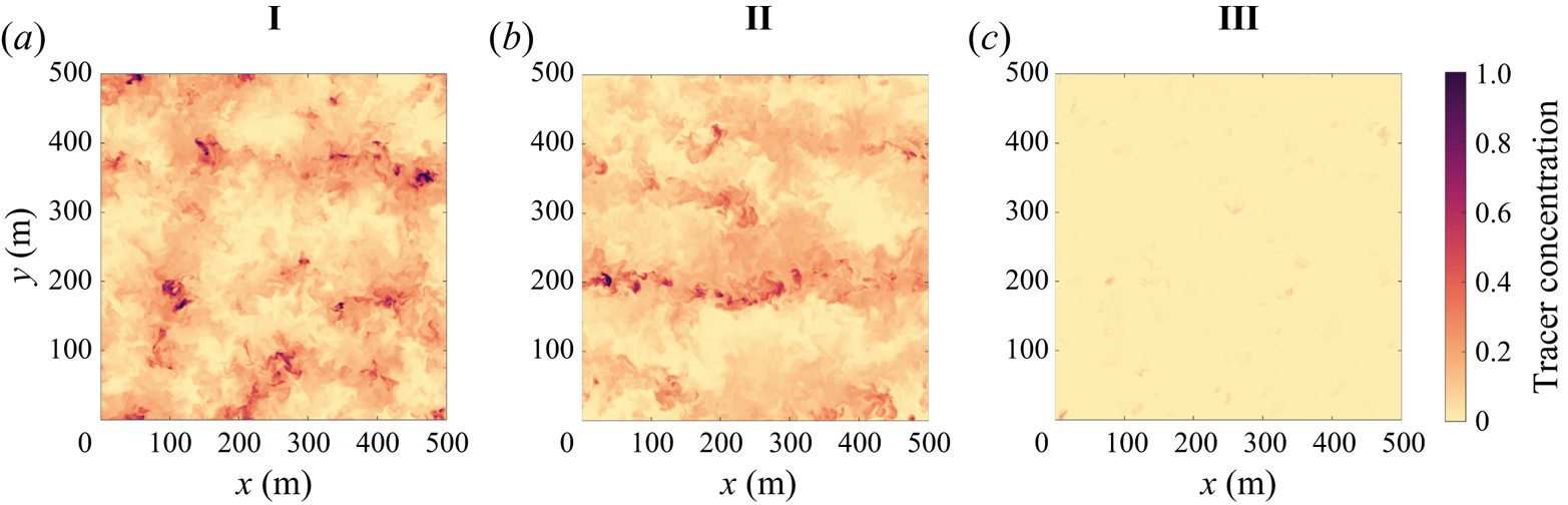
Figure 5. Horizontal cross-section at  $z=-30$ m of the buoyant tracer concentration ( $w_s=0.005$ m s $^{-1}$).
3.2. Convective vortices
In this section we examine the convective vortices in more detail, focusing in particular on the influence of wind forcing on the convective vortices. There are several ways to identify convective vortices. Chor et al. (Reference Chor, Yang, Meneveau and Chamecki2018a) characterised convective vortices using the 2-D Okubo parameter. Here, we apply a similar method as developed in Raasch & Franke (Reference Raasch and Franke2011) who identified dust devils in a convective boundary layer using pressure and vorticity. Whilst vorticity is an obvious measure, small-scale turbulence also contributes to vorticity, making it difficult to identify coherent convective vortices. We eliminate some of this small-scale noise by applying a Gaussian filter to the vorticity field before using it to identify convective vortices. In addition, structures such as regions of high shear can have large values of vorticity, and so we use the pressure field in conjunction with vorticity to exclude such structures. The physical reasoning behind using the pressure field is that the centrifugal force created by the fluid rotating inside the vortex causes the pressure to be lower than the surrounding fluid (Hussain & Jeong Reference Hussain and Jeong1995). We have verified that pressure and the Okubo parameter yield qualitatively similar results (see Appendix B).
Vortices are identified using the local minima of the departure from the hydrostatic pressure and local maxima of the filtered absolute vorticity field, where local minimum/maximum means that the values are smaller/larger than the adjacent 224 grid points (forming a  $15 \times 15$ grid). This grid size has been determined empirically to avoid detection of multiple vortex centres within one convective vortex. We use the pressure and vorticity fields evaluated at $z=-1$ m to match the depth of the surface particles. We require the pressure minimum to be located within two horizontal grid points of the filtered absolute vorticity maximum, which we define as the vortex centre. We use a threshold value of five times the standard deviation of filtered absolute vorticity ( $5\sigma _{\zeta }$) and five times the standard deviation of perturbation pressure ( $5\sigma _p$) at $z=-1$ m, which is similar to the applied thresholds in other vortex detection algorithms (Nishizawa et al. Reference Nishizawa2016; Giersch et al. Reference Giersch, Brast, Hoffmann and Raasch2019). This threshold aims to eliminate as much non-coherent turbulence as possible, whilst still capturing sufficient information for analysis. The magnitude of the threshold value depends on the strength of wind forcing and convective forcing of each simulation.
More convective vortices are identified under strong convective conditions, and the number of convective vortices decreases with increasing wind strength. To quantify this in all simulations, we count the number of vortices detected using our criterion at each time step and average over one inertial period. Figure 6 shows that the total number of vortices decreases as  $u^*/w^*$ increases. In case I there are approximately two vortices per 100 m $^{2}$ (40 vortices in the 500 m $^2$ domain). When $u^* \simeq w^*$ (case II), the number decreases by about two orders of magnitude compared with when $u^*=0$ (case I). For higher values of $u^*/w^*$, less than one vortex is detected in the domain at any given time. Note that the number of convective vortices is not exactly equal to zero when $w^*=0$. We interpret this as rare regions of intense turbulence that happen to meet our criterion rather than as convective vortices.
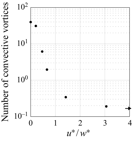
Figure 6. Ratio of  $u^*$ and $w^*$ against the number of vortices detected at any given time averaged over one inertial period in the full domain ( $500\ {\rm m} \times 500\ {\rm m}$). The arrow indicates the number when $u^*/w^*$ is infinite.
To visualise the convective vortices in cases I, II and III, we use the pressure field. Figure 7 shows pressure isosurfaces in the upper panel and pressure contours at  $z=0$ (black) and particle position (red) in the lower panel. In cases I and II we observe coherent convective vortices that typically occur in the regions of strong downwelling and extend down from the surface into the mixed layer. Note, however, by comparison with figure 2, that not all locations with strong downwelling contain a convective vortex. In case I the convective vortices occur in the nodes where downwelling regions join together and there is coincident particle clustering inside the convective vortices. In case II the convective vortices preferentially occur in the coherent downwelling streaks and are tilted in the direction of wind forcing. Surface particles cluster in the larger downwelling streaks and are less confined to convective vortices than in case I. In case III coherent vortices are not visible and there is relatively little particle clustering. In all cases, the convective vortices detected have a relatively small diameter of a few metres. This implies that simulations need a high resolution for convective vortices to be visible and observations in the ocean would require measurements at small scales.
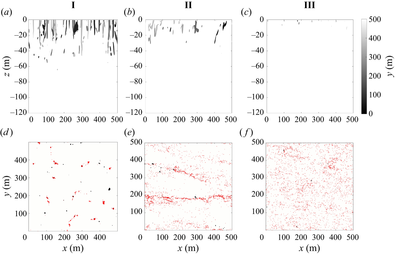
Figure 7. (a)–(c) Spanwise view of pressure isosurfaces where the departure from the hydrostatic pressure is  $\delta = 5 \times \sigma _p$ Pa, taken at $t=12$ hours. All regions with $\delta p< 5 \times \sigma _p$ Pa are visible in this view. (d)–( f) Horizontal cross-section of the pressure contour at $z=-1$ m (black) with surface particle position superimposed (red), taken at $t=12$ hours.
To further characterise the surface flow, we look at the relationship between vertical velocity and pressure. This allows us to identify regions of downwelling and convective vortices, both of which have a role in clustering buoyant material. The joint probability distribution function of vertical velocity and pressure is shown in figure 8 under different wind and convective forcing at  $z=-1$ m. In all cases, points that have values of vertical velocity and pressure near zero are much more common than points with extreme values. In case I the distribution of points is highly skewed, with a long tail of values with negative pressure. The contour at probability density level $10^{-4}$ demonstrates that there are more points with negative pressure and negative vertical velocity. This indicates that convective vortices experience a bias towards downwelling circulation, which is consistent with the visualisations (figure 7d).
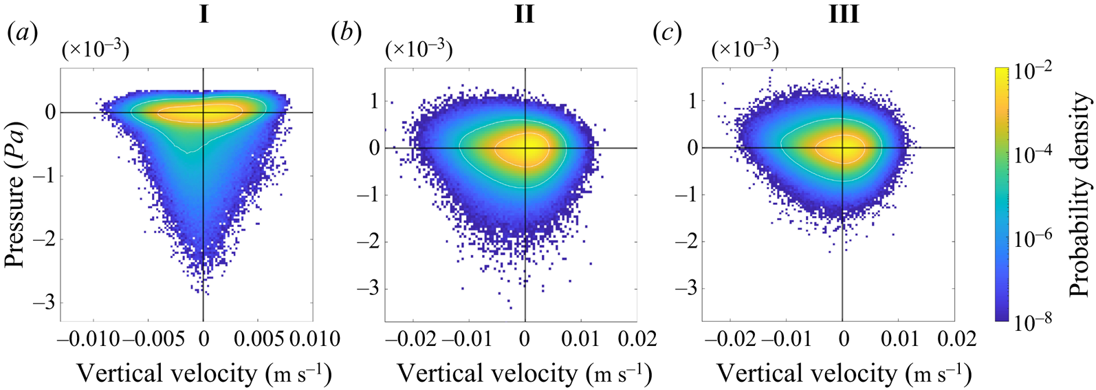
Figure 8. Joint PDF of the vertical velocity and pressure perturbation ( $\delta p$) at $z=-1$ m. White contours show where the PDF is $10^{-2}$ and $10^{-4}$.
With wind forcing (cases II and III), the shape of the joint probability density function (PDF) becomes more isotropic, in particular in the distribution of pressure points between positive and negative values. The range in vertical velocity is larger in case II and III compared with case I (note the change in axis limits). Case II has more points with low pressure than case III, consistent with the visualisation showing well-defined convective vortices in case II but not case III, and the very small number of vortices detected (figure 6).
We can analyse the mean structure of the convective vortices by superposing many convective vortices and averaging their properties. For each time step, we identify convective vortices using the detection method described above and average the field centred at the vortex centre over all of the vortex centres found during one inertial period.
Figure 9 shows horizontal (a) and vertical (b) slices of the vertical velocity for the averaged convective vortex in case I. The horizontal cross-sections are taken at  $z=-1$ m whilst the vertical cross-sections are taken through the centre of the averaged convective vortex. The threshold pressure contour (red) is included along with the vectors of horizontal velocity (black).
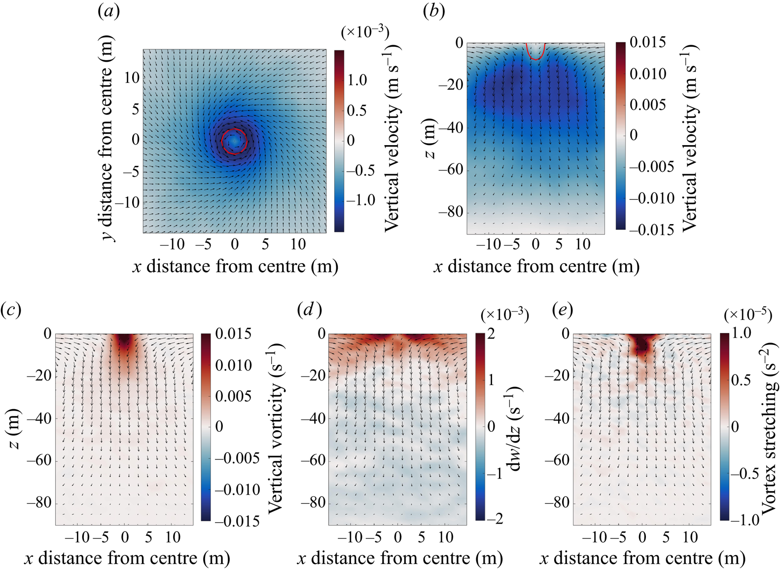
Figure 9. Horizontal cross-section of the vertical velocity at  $z=-1$ m (a) and vertical cross-sections of the vertical velocity (b), vertical vorticity (c), $\partial w / \partial z$ (d) and vertical vortex stretching (e) for the averaged vortex in case I with vectors of horizontal velocity (black) and the threshold pressure contour (red).
The averaged convective vortex is symmetric about its centre. Although the mean vortex diameter is about 5 m based on the pressure threshold, enhanced subduction extends about 15 m from the vortex centre. Since the vortex diameter is only several times larger than the model grid spacing, it is possible that the vortex diameter would be even smaller in higher resolution simulations. The mean flow spirals inwards to the centre of the convective vortex with cyclonic (counterclockwise) rotation. The peak vertical velocity occurs on the periphery of the convective vortex and encircles a local minimum in the centre. This is consistent with simulations of dust devils in the atmosphere (Raasch & Franke Reference Raasch and Franke2011; Giersch & Raasch Reference Giersch and Raasch2021), which speculate that the decrease in vertical velocity in the central core of an averaged vortex could indicate stagnation points or flow reversal inside dust devils, shown schematically in Balme & Greeley (Reference Balme and Greeley2006). Such features may be observable in instantaneous data with higher resolution, but this is outside the scope of the current study. Below 30 m the downwelling broadens and becomes weaker in the bottom half of the mixed layer.
The convective vortices are maintained by vortex stretching. The vertical component of the vortex stretching term is  ${\boldsymbol \omega } \boldsymbol {\cdot } \boldsymbol {\nabla } w$, where ${\boldsymbol \omega }=\boldsymbol {\nabla } \times {\boldsymbol u}$ is the vorticity and $w$ is the vertical velocity. Figure 9(c–e) shows the vertical component of vorticity, $\zeta, \partial w/\partial z$, and $\zeta \times \partial w/\partial z$ all averaged over the ensemble of convective vortices. The term ${\boldsymbol \omega } \boldsymbol {\cdot } \boldsymbol {\nabla } w$ is dominated by stretching of vertical vorticity ( $\zeta \times \partial w/\partial z$), whilst the vortex twisting term ( $\zeta _x \partial w/\partial x + \zeta _y \partial w/\partial y$) is one order of magnitude smaller and shows little coherence. The ensemble mean is characterised by large vertical vorticity near the surface that decreases with depth. Interestingly, the average vorticity is positive, which indicates a bias towards cyclonic rotation as explored further below. The vertical component of the vortex stretching term is positive in the core of the mean vortex, indicating a source of positive vertical vorticity. Below 30 m, $\partial w/\partial z$ changes sign and there is little coherence in the vortex stretching field. The relatively small positive vorticity below 30 m is likely maintained by advection or diffusion.
The structure of the convective vortex changes as the wind stress increases. Figure 10 shows horizontal (a–d) and vertical (e–h) cross-sections of the vertical vorticity averaged over the ensemble of convective vortices for  $\tau = 0$ (case I), $0.01,\ 0.05,\ 0.1$ Nm $^{-2}$ (case II), with the buoyancy flux remaining constant ( $B_0=-4.24 \times 10^{-8}$ m $^2$ s $^{-3}$). The remaining simulations do not have a large enough number of convective vortices to provide a robust average (see figure 6) and are not shown. As wind forcing increases, the horizontal vortex structure becomes less symmetric and we observe a streak of increased vorticity that extends from the vortex centre in the direction of wind forcing. Under these higher wind strengths, the vortex tilts and is confined to shallower depths that is consistent with the shearing of the convective vortices seen in figure 7. Interestingly, the magnitude of vorticity inside the convective vortex is not strongly dependent on the strength of the wind forcing, and the bias towards positive vorticity also persists.

Figure 10. Horizontal (a–d) and vertical (e–h) cross-sections of the vertical vorticity for the averaged vortex for  $\tau = 0, 0.01, 0.05, 0.1$ Nm $^{-2}$ with vectors of horizontal velocity superimposed.
Despite their small size, the convective vortices in our simulations exhibit a strong bias towards cyclonic (counterclockwise in the northern hemisphere) rotation, suggesting an influence from the Coriolis acceleration. The relative importance of the Coriolis acceleration is typically quantified using the Rossby number,  $Ro\equiv U/(fL)\sim \zeta /f$. It is generally assumed that the planetary rotation is unimportant for processes that are characterised by $Ro\gg 1$. Here, $\zeta /f>100$ within the convective vortices in case I, and hence, the bias towards cyclonic rotation is surprising. Although there has been some debate, observations and simulations of dust devils in the atmosphere appear to indicate that cyclonic and anticyclonic vortices form in roughly equal number (Sinclair Reference Sinclair1965; Balme & Greeley Reference Balme and Greeley2006). In the oceanic case, Chor et al. (Reference Chor, Yang, Meneveau and Chamecki2018a) set $f=0$ and, hence, did not explore the possibility of a cyclone/anticyclone asymmetry. Similar observations of a rotational bias within a high Rossby regime have been recorded in experiments and simulations of convective plumes in a rotating environment (Frank et al. Reference Frank, Landel, Dalziel and Linden2017; Sutherland et al. Reference Sutherland2021).
Figure 11 shows the PDF of the vertical vorticity at  $z=0$ for points associated with convective vortices (left) and for all points in the domain (right) over one inertial period. To remove turbulent fluctuations, the vorticity at each point is averaged over a box measuring approximately $5$ m
$5$ m $\times 5$ m, which is a similar length scale to the diameter of a convective vortex. In addition to cases I ( $\tau =0$ Nm $^{-2}$) and II ( $\tau =0.1$ Nm $^{-2}$), we show the vorticity distribution for the two simulations with intermediate wind stress $\tau =0.01$ Nm $^{-2}$ and ${\tau =0.05}$ Nm $^{-2}$, with the buoyancy flux remaining the same ( $B_0=-4.24 \times 10^{-8}$ m $^2$ s $^{-3}$).
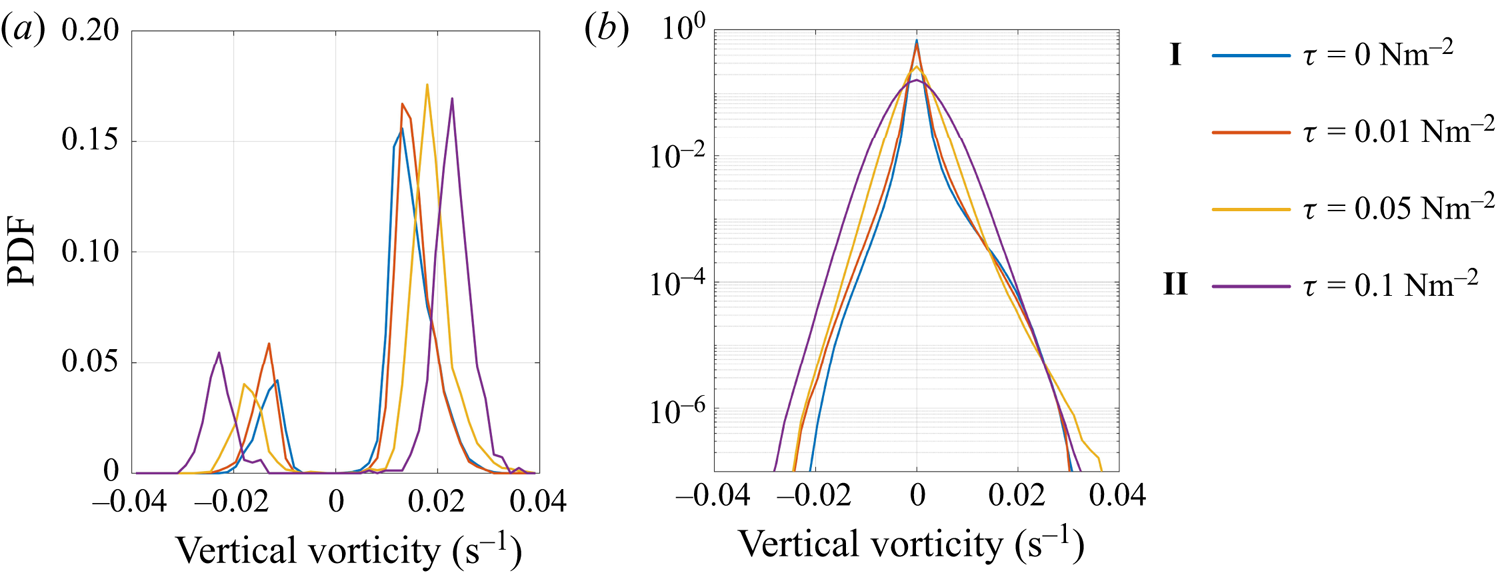
Figure 11. Probability density function of the vertical vorticity at  $z=0$ for points identified as convective vortices (a) and all points in the domain (b).
In case I the PDF shows a distinct peak at  $\zeta \simeq \pm 0.015$ that agrees with the ensemble mean shown in figure 10. All cases show a bias towards cyclonic vorticity, and for ${\tau =0}$ Nm $^{-2}$ and $\tau =0.01$ Nm $^{-2}$, there is a noticeable bias in the distribution of vorticity for all points in the domain. As the wind stress increases, the peak in vorticity has a larger magnitude. This is likely due to the increased standard deviation of filtered vorticity in the stronger wind cases, leading to a larger threshold value used to identify convective vortices.
To explain the cyclonic bias, it is useful to examine the evolution of vorticity along the trajectory of surface particles. In the absence of friction, the vertical component of the vorticity evaluated along the paths of Lagrangian particles at  $z=0$ satisfies
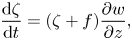 \begin{equation} \frac{{\rm d}\zeta}{{\rm d}t}=(\zeta+f) \frac{\partial w}{\partial z},\end{equation}
where  $\zeta$ is the vertical component of the vorticity vector and $f$ is the constant Coriolis parameter.
We can obtain a useful approximation if we use a constant value for  $\partial w/\partial z$ to characterise the flow within a convective vortex. In the limit when $|\zeta |\ll |f|$ (corresponding to early times when particle vorticity is very small), (3.1) then yields
 \begin{equation} \zeta=\zeta_0+f\frac{\partial w}{\partial z}t,\end{equation}
where  $\zeta _0$ can be interpreted as the vorticity when the particle first encounters the convective vortex.
Sutherland et al. (Reference Sutherland2021) used a similar argument, along with a scaling for  $\partial w/\partial z$, to explain the unexpected influence of rotation on high-Rossby-number plumes in a rotating environment observed in lab experiments reported earlier in Frank et al. (Reference Frank, Landel, Dalziel and Linden2017). Following their arguments, we can estimate the time scale needed for a particle that initially has no vorticity to reach a state with $\zeta \simeq |f|$. Using $\partial w/\partial z\simeq 2\times 10^{-3}\ \mbox {s}^{-1}$ (figure 9d) gives a time scale of about 8 minutes. In § 3.3 we quantify the time a particle spends inside a convective vortex using particle statistics and find that in case I particles remain within a convective vortex for an average of 47 mins. This suggests that particles spend enough time within convective vortices for the planetary rotation to become important even if a particle enters a vortex with no relative vorticity.
The argument above holds when  $|\zeta |\ll |f|$. However, the mean vorticity within convective vortices greatly exceeds $f$ (figure 10). Returning to (3.1) and taking $|\zeta | \gg f$ while again using a constant value for $\partial w/\partial z$ yields solutions with exponentially increasing vorticity,
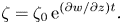 \begin{equation} \zeta=\zeta_0 \,{\rm e}^{({\partial w}/{\partial z})t}.\end{equation}
 To examine the applicability of the linear and exponential solutions for vorticity, we evaluate the vorticity along trajectories of surface particles. For each particle, the pressure and vertical vorticity are interpolated at every time step using cubic B splines. We identify the time when each particle enters a convective vortex as the time when the particle pressure falls below  $5 \sigma _p$ and the particle filtered vorticity falls below $5 \sigma _{\zeta }$ (the same criterion as used to identify convective vortices) and remains below this threshold for 30 mins when $\tau =0$ Nm $^{-2}$ (case I) and 10 mins when $\tau =0.05$ Nm $^{-2}$. We then average the vorticity sampled along each particle path as a function of time referenced to the time when the particle entered the convective vortex (labelled $t=0$). Figure 12 shows the time series of the average vorticity sampled along the surface particle paths for $\tau =0$ Nm $^{-2}$ and $\tau =0.05$ Nm $^{-2}$, where we also show the linear and exponential growth solutions using $\partial w /\partial z = 2\times 10^{-3}$ s $^{-1}$. We have verified that, for $\tau =0.01$ Nm $^{-2}$, the time series of the average vorticity is similar to case I, whilst for $\tau =0.1$ Nm $^{-2}$, the particles do not enter enough convective vortices to provide a meaningful average.
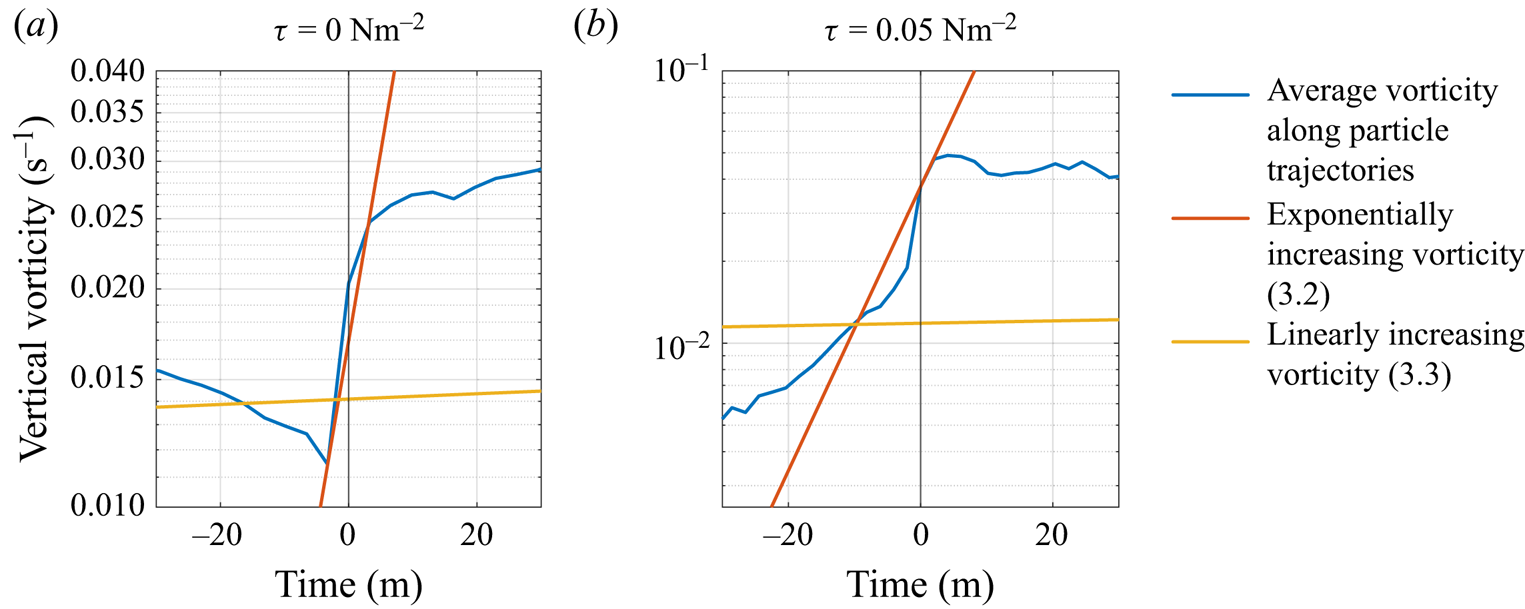
Figure 12. Average trajectory of  $\zeta$ along a surface particle path against the time spent inside a convective vortex (blue) with the exponential (red) and linear (yellow) vorticity solutions superimposed. Time $t=0$ corresponds to the time at which the particle enters a convective vortex.
In both cases, the sudden increase in vertical vorticity just before the particle enters a convective vortex is consistent with an exponential increase in vorticity at a rate set by the value of  $\partial w/\partial z$ given above. Even before entering a convective vortex, particles are biased towards cyclonic vorticity from vortex stretching acting on the planetary vorticity (3.2). During each vortex encounter, the vorticity sampled along particle paths exponentially increases due to vortex stretching. Shortly after the particles enter the convective vortices, the vertical vorticity saturates. It is likely that frictional dissipation (which we neglected in (3.1)) competes with vortex stretching to prevent the relative vorticity from increasing further. A full exploration of the dynamics of convective vortices including frictional effects is left for a future study.
3.3. Clustering of buoyant material
In this section we analyse the influence of convective vortices on the accumulation of buoyant material. We start by looking at the distribution of a buoyant tracer in the flow and then analyse the trajectories of surface particles. Finally, we introduce a measure to quantify buoyant material clustering and give an overview of clustering for all simulations.
Figure 13 shows the horizontal and vertical slices of the tracer concentration averaged over the ensemble of convective vortices for  $\tau = 0, \ 0.01,\ 0.05,\ 0.1$ Nm $^{-2}$. In case I the concentration of the buoyant tracer is highest at the surface and inside the convective vortex, and the tracer concentration decreases with distance from the vortex centre. Interestingly, the maximum buoyant tracer concentration does not coincide with the region of maximum downwelling (figure 9a,b) but with the maximum vorticity. The reason for this is not clear, but we explore the relation between vertical velocity, pressure and tracer concentration further below. Under strong wind forcing, the maximum tracer concentration occurs upstream of the vortex centre and tracer accumulates in a horizontal streak oriented in the direction of wind forcing. We observe vertical shearing of the vortex similar to the vorticity field (figure 10) and there is less tracer at depth under stronger wind forcing.
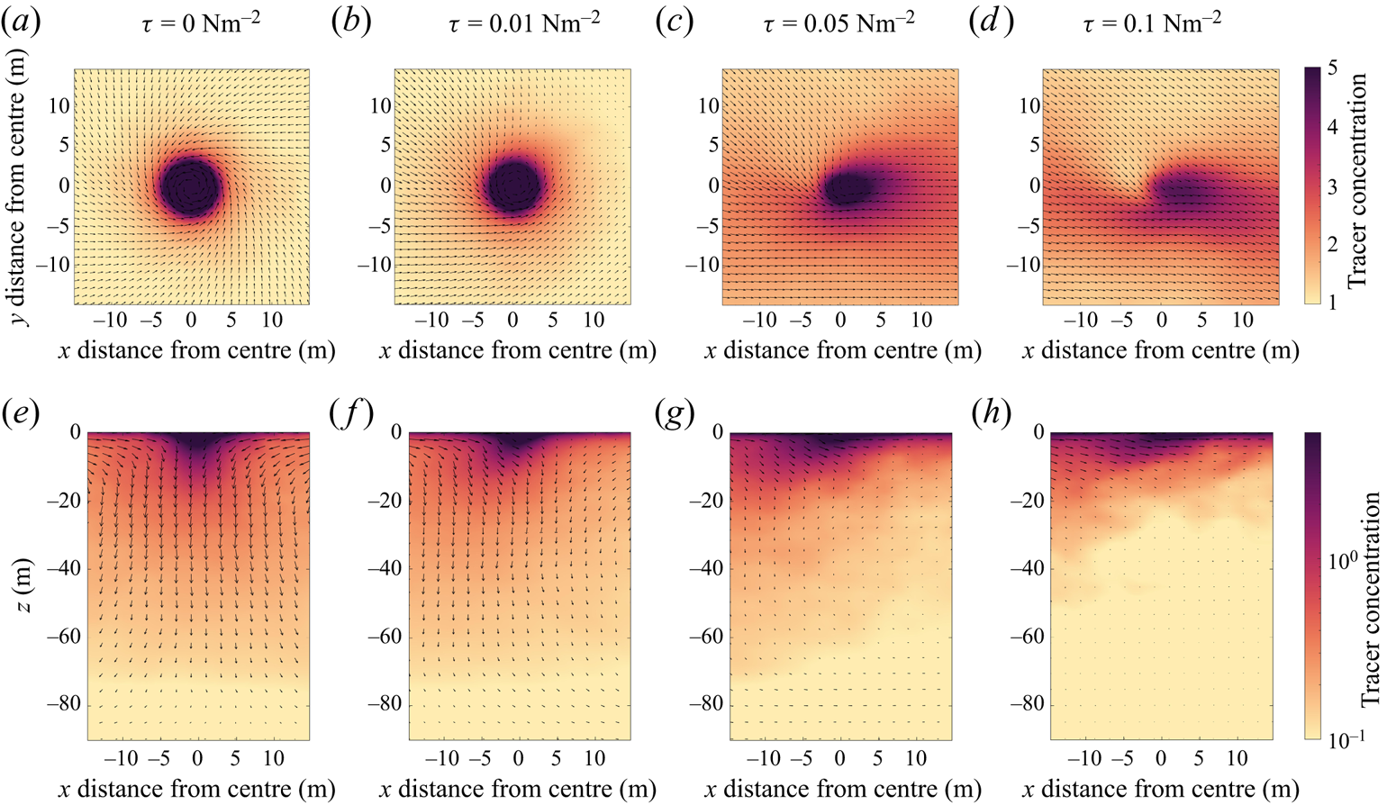
Figure 13. Horizontal (a–d) and vertical (e–h) cross-sections of the tracer concentration ( $w_s=0.005$ m s $^{-1}$) for the averaged vortex for $\tau = 0, 0.01, 0.05, 0.1$ Nm $^{-2}$ with vectors showing velocity in the x–z plane superimposed.
The cyclonic convective vortices are more effective at accumulating buoyant particles than the anticyclonic vortices. To quantify this, we count the number of particles inside each convective vortex identified using our vortex detection criterion, where a particle is counted as being inside a vortex if it is located within a  $15 \times 15$ grid (corresponding to $14.25\ {\rm m} \times 14.25$ m grid) centred at the vortex centre. We find that in case I the average number of particles inside a cyclonic vortex is 23, whilst the average number of particles inside an anticyclonic vortex is 6. This bias continues up to $\tau =0.01$ Nm $^{-2}$ with the buoyancy flux remaining constant ( $B_0=-4.24 \times 10^{-8}$ m $^2$ s $^{-3}$). Beyond this, we do not observe enough particles accumulating inside the convective vortex to give a statistically significant result. We see a similar pattern with the tracer field. Although the average tracer concentration ( $w_s=0.005$ m s $^{-1}$) is qualitatively similar in cyclonic and anticyclonic convective vortices, the tracer concentration is much higher inside the cyclonic vortices (maximum surface tracer concentration in the averaged cyclonic vortex is three times higher than in the averaged anticyclonic vortex for case I).
In convective dominated simulations we observe buoyant material accumulating inside convective vortices rather than downwelling regions (figures 2d and 13). Figure 14 shows the concentration of the buoyant tracer with  $w_s=0.005$ m s $^{-1}$ at $z=0$ m, averaged in bins based on the vertical velocity and pressure at $z=-1$ m. In case I the buoyant tracer has a strong tendency to accumulate in regions with negative pressure that characterise convective vortices. This effect is dominant over the preference for particles to accumulate in regions with negative vertical velocity. This result is in line with the findings from Chor et al. (Reference Chor, Yang, Meneveau and Chamecki2018a). The large variability of tracer concentration at the edge of the distribution is associated with averaging over a small number of points (see figure 8). Outside the convective vortices the regions with positive vertical velocity (above 0.002 m s $^{-1}$) have a very low tracer concentration, which is consistent with the visualisation in figure 2(d).
Figure 14. Concentration of the buoyant tracer ( $w_s=0.005$ m s $^{-1}$) at $z=0$ conditioned to pairs of vertical velocity and pressure perturbation ( $\delta p$) at $z=-1$ m.
When wind forcing is present (cases II and III), the tracer is more uniformly distributed across pressure and vertical velocity and there are fewer extremes in the tracer concentration (note the difference in colour axis for these panels). In both cases there is a distinct minimum in the tracer concentration in regions with positive vertical velocity. When convection and wind are both present (case II), the tracer concentration is large in regions of strong downwelling and low pressure. The notable difference in the tracer distribution in cases I and II shows that although convective vortices are present in case II, they are not as effective at accumulating buoyant tracers compared with the convective vortices in case I.
Although the buoyant tracer does not accumulate as effectively inside the convective vortices under strong wind forcing, we see accumulation inside streaks of high speed. Figure 15(a–c) shows the concentration of the buoyant tracer with  $w_s=0.005$ m s $^{-1}$ at $z=0$ m, averaged in bins based on the vertical velocity and squared horizontal speed ( $u^2 + v^2$) at $z=-1$ m. In case III the concentration of the buoyant tracer is highest in regions of high speed, even when the vertical velocity is positive. In case II the tracer is more uniformly distributed (note change in colour axis) but there are still elevated concentrations in regions of high speed. This is consistent with the close resemblance of horizontal distribution of speed (figure 15d–f) and buoyant tracer (figure 2e, f), both of which show clear streaks with elevated speed/tracer concentration.
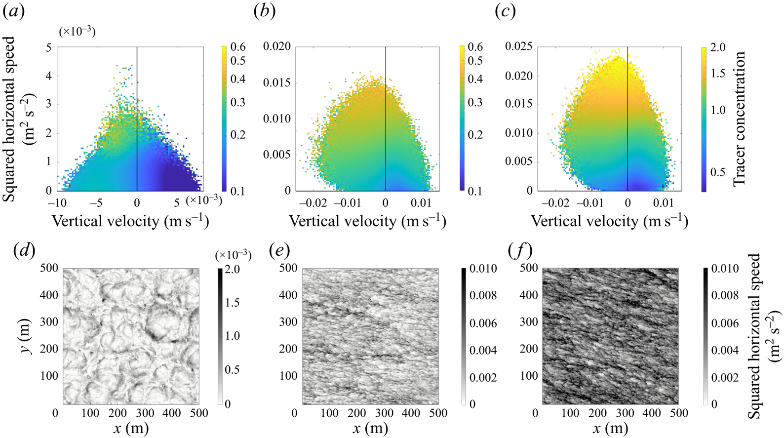
Figure 15. Buoyant tracer concentration ( $w_s=0.005$ m s $^{-1}$) conditioned to pairs of vertical velocity and squared horizontal speed ( $u^2 + v^2$) at $z=-1$ m (a–c). Horizontal cross-sections of squared horizontal speed at $z=-1$ m at $t=12$ hours (d–f).
When wind forcing is removed (case I), there is a clear difference in tracer distribution amongst speed and vertical velocity points. We see a distinct minimum tracer concentration when vertical velocity is positive (similar to figure 14a). There is a small set of points that have a high tracer concentration and large values of speed, and from figure 15(d) we see that these correspond to convective vortices that have high speed on the periphery.
We can use the surface particles to describe the statistics of particle encounters with convective vortices. We calculate the time that a particle spends inside a convective vortex based on the time that the pressure sampled along the particle path is below the threshold value ( $5 \sigma _p$) and the filtered absolute vorticity sampled along the particle path is above the threshold value ( $5\sigma _{\zeta }$). We repeat this for 4000 particles over one inertial period. We also measure the distance that each particle is transported by the convective vortices. This is done by calculating the Euclidean distance between the point where the particle first falls below the pressure threshold value and the last point where the particle pressure is below the threshold value before increasing. In a similar way, we calculate the time spent and distance travelled by a particle outside of a convective vortex. This is the period after a particle has just been expelled from a convective vortex (pressure or filtered vorticity are below/above threshold values) until it next enters another convective vortex. Some key statistics from these calculations are given in table 2 for each of the three cases.
Table 2. Statistics from individual surface particle trajectories for time and distance travelled inside (upper half) and outside (lower half) a convective vortex.
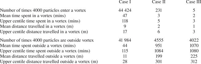
In case I particles enter and exit convective vortices frequently. On average, particles enter a convective vortex more than 10 times during one inertial period and particles spend a similar amount of time inside and outside convective vortices. This latter statistic is remarkable considering the relatively small area occupied by convective vortices (see figure 2h). The time that particles spend in a convective vortex can be compared with the convective time scale. This is defined as  $t_c=h/w^*$ and provides a characteristic time scale for the mean circulation within convective cells. In case I, $t_c\simeq 88$ mins, which is comparable to the average time that particles spend inside a convective vortex. This suggests that, in this case, convective vortices trap particles for a period of time that is significant compared with the convective time scale. In addition, the average distance that particles travel during periods inside and outside of convective vortices is small compared with the 50–150 m size of convective cells (see figure 2). This suggests that convective vortices do not travel long distances sweeping up particles as suggested in Chor et al. (Reference Chor, Yang, Meneveau and Chamecki2018a), but rather that particles remain close to the convective vortices in the convective nodes.
The addition of wind disrupts the effectiveness of convective vortices at trapping particles, which can be seen by the contrast in statistics in cases II and III. Most particles do not enter a convective vortex at all, and upon entering, particles spend just 2–3 mins on average inside the convective vortices. This is much smaller than both the average time spent outside convective vortices and the convective time scale, which is also 88 mins for case II. In cases II and III particles travel much further outside convective vortices than inside the vortices, and the distance travelled outside is comparable to the scale of the wind streaks. This suggests that the dynamics outside the convective vortex are much more important in determining particle distribution compared with case I.
A physical explanation for the clustering of surface particles inside convective vortices is as follows. Convective vortices preferentially occur in the ‘nodes’ linking the downwelling regions of neighbouring convection cells. Particles that are brought into the convection nodes by convergent surface currents are pulled into the centre of the convective vortex by the inwards spiralling flow. In pure convection and under additional weak wind forcing, convective vortices are able to collect many neighbouring particles that, on average, remain trapped inside the vortex for a relatively long time compared with the convective time scale and only travel a short distance inside the vortex. When a convective vortex eventually breaks up, it leaves behind a cluster of particles inside the convective nodes that tend to stay close together since their local flow field is the same. The cluster may then fall into another nearby convective vortex, which attracts additional particles and further increases clustering.
The degree of clustering for buoyant tracers and surface particles can be quantified using the Gini coefficient (Gini Reference Gini1912). For a sample of size  $n$ where observed values $y_i (i=1,\ldots, n)$ are in non-decreasing order ( $y_i\leq y_{i+1}$), the Gini coefficient is defined as
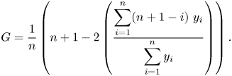 \begin{equation} G = \frac{1}{n} \left( n+1-2 \left(\frac{\displaystyle \sum_{i=1}^{n} (n+1-i) \ y_i}{\displaystyle \sum_{i=1}^{n} y_i} \right) \right).\end{equation}
 A Gini coefficient close to 0 indicates a uniform distribution, while a value close to 1 indicates strong clustering. For the surface particles, we calculate the Gini coefficient using the number of particles within boxes formed of  $32 \times 32$ grid points (or $31.25\ \mbox {m} \times 31.25\ \mbox {m}$) at each time step, and we average the Gini coefficient over one inertial period. This box size has been chosen because it characterises clustering at a scale that captures the two most extreme behaviours of our simulation: under strong convective forcing, 31.25 m is small enough to distinguish clustering in different vortices, while under strong wind forcing, it captures the larger-scale behaviour when there is less clustering.
Figure 16(a) shows that the Gini coefficient for surface particles decreases as the ratio  $u^*/w^*$ increases. The limited number of particles in our simulations implies that the particles will not be evenly distributed between the boxes even if the particle distribution is purely random. To quantify this and provide a baseline for comparison, we calculate the Gini coefficient for a set of particles that have been randomly distributed. To do this, we randomly distribute 4000 particles throughout the domain and calculate the Gini coefficient using (3.4). We repeat this process 500 times and the dashed line in figure 16(a) indicates the average of the resulting Gini coefficients for random distributions. The particles in the wind dominated regime (III) exhibit more clustering than would be seen for a random distribution of the same number of particles (dashed line), suggesting that some clustering still occurs in the wind-forced case. The ratio of $u^*$ and $w^*$ against the Gini coefficient closely resembles the ratio of $u^*$ and $w^*$ against the instantaneous number of vortices (figure 6) and suggests that fewer convective vortices leads to less particle clustering.
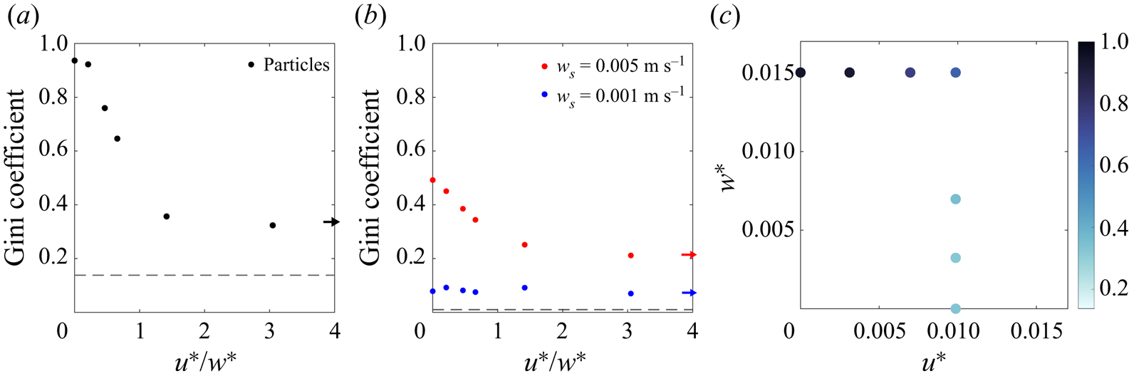
Figure 16. Ratio of  $u^*$ and $w^*$ against the Gini coefficient averaged over one inertial period for surface particles (a) and the buoyant tracer (b). The dashed line indicates the Gini coefficient for a random distribution. The arrow indicates the Gini coefficient for case III where the ratio is infinite. (c) Parameter space coloured by Gini coefficient for surface particles.
For the buoyant tracer, we apply the Gini coefficient to the total tracer concentration within boxes composed of  $32\times 32$ grid points (same clustering scale as above) at each time step and average over one inertial period. For comparison with a random distribution of tracer, we generate a uniformly random concentration at each grid point on the $512\times 512$ grid and calculate the Gini coefficient using (3.4), averaged over 500 samples. The slip velocity has a significant impact on tracer clustering as can be seen in figure 16(b). Under all forcing conditions, the strongly buoyant tracer (red) is more clustered than the weakly buoyant tracer (blue). For the strongly buoyant tracer, the Gini coefficient trend is very similar to that for surface particles: the Gini coefficient decreases as the wind to convection ratio increases. The Gini coefficient for the weakly buoyant tracer is not strongly affected by the strength of wind or convection, but the distribution is still distinct from a random distribution of tracer (dashed line). Even in case I ( $u^*/w^*=0$) the convective vortices that effectively trap surface particles do not cause strong accumulation for the weakly buoyant tracer.
Figure 16(c) shows the particle Gini coefficient as a function of  $u^*$ and $w^*$. This enables us to separate out the behaviour for increasing wind strength and increasing convective forcing. Recall that the simulations are initialised with the same reference density and mixed layer depth, and hence, changes in $u^*$ and $w^*$ (calculated with constant $h=80$ m) reflect changes in the surface wind stress and the surface buoyancy flux, respectively.
In the series of simulations with constant wind stress (vertical line of points in figure 16c), increasing the magnitude of surface cooling leads to more clustering and a larger Gini coefficient, while increasing the wind stress for a fixed level of convective forcing (horizontal line of points) results in a decrease in the Gini coefficient. Although it is tempting to draw conclusions about the value of the Gini coefficient on lines of constant  $u^*/w^*$, only a small section of the parameter space has been covered by our simulations. It remains unclear whether the Gini coefficient can be described purely as a function of $u^*/w^*$.
4. Conclusions
In this study we used idealised LES to investigate the distribution of buoyant material in the ocean under combined wind and convection forcing. Convective turbulence was generated using a constant buoyancy flux at the surface and wind forcing was generated using a constant shear stress boundary condition applied at the surface ( $z=0$). A series of simulations were conducted with different strengths of wind and convective forcing. We used two approaches to model buoyant particles: a continuous Eulerian tracer field with an upwards slip velocity and Lagrangian particles that were confined to the surface. The tracer field allowed us to look at the distribution of particles with vertical motion included, whilst the surface particles allowed us to look at the limit where the slip velocity exceeds the maximum flow speed. The flow dynamics and subsequent clustering of buoyant material depend on wind and convection forcing, which we characterised with the ratio of the frictional velocity and convective velocity $u^*/w^*$.
The horizontal distribution of buoyant material depends strongly on the slip velocity. Weakly buoyant tracers are relatively uniformly distributed at the surface and are advected deeper in the turbulent mixed layer. We used the Gini coefficient to characterise clustering and found that clustering decreases with increasing wind strength, while it increases with increasing convection strength. On the other hand, weakly buoyant tracers remain nearly uniformly distributed regardless of the strength of wind or convection forcing.
In the simulations with strong convection, convective vortices form in the ‘nodes’ that join regions of downwelling in neighbouring convective cells. In the absence of wind forcing, convective vortices are highly effective at accumulating surface particles and strongly buoyant tracers. Convective vortices also act to transport the buoyant tracer deep into the mixed layer. This is consistent with the findings from Chor et al. (Reference Chor, Yang, Meneveau and Chamecki2018a) who considered simulations of buoyant tracers in convection without wind forcing.
Although convective vortices survive under strong wind forcing, they become less effective at clustering buoyant material as the wind stress increases. As wind forcing is increased under a convective regime, we observe fewer convective vortices and a transition from clustering inside convective vortices to clustering inside streaks of high speed. When convective forcing is removed, the buoyant tracers remain close to the surface and some clustering occurs due to accumulation in regions of high speed and downwelling regions.
Surprisingly, the convective vortices exhibit a bias towards cyclonic vorticity despite their small size and the fact that they are characterised by very large Rossby numbers. The vorticity sampled along particle paths increases exponentially as the particles enter convective vortices. This is consistent with a simple theory for the vorticity amplification using the vertical divergence ( $\partial w/\partial z$) measured near the convective vortices. A similar argument was put forward by Frank et al. (Reference Frank, Landel, Dalziel and Linden2017) and Sutherland et al. (Reference Sutherland2021) to explain rotational effects on buoyant plumes from a fixed source. This might help explain how a cyclonic bias first develops, but their assumption that $|\zeta |\ll f$ (small Rossby number) and the predicted linear increase in vorticity are not consistent with our simulations.
The picture that emerges is that surface particles that accumulate in the nodes between convection cells frequently encounter convective vortices. The first time that a particle encounters a convective vortex, the planetary vorticity is amplified, leading to a bias towards cyclonic vorticity. With each subsequent encounter, the relative vorticity is ‘ratcheted’ up. Eventually this increase is balanced by the removal of vorticity through viscosity, although we have not investigated this balance and we leave this for future work.
It is important to keep in mind potential limitations of the current study. In our simulations, we held the surface forcing constant. In the ocean, the surface heat flux and wind stress are often highly variable, and this variability could impact the distribution of buoyant material. Here, we also focused solely on the effects of convection and wind-driven turbulence and neglected many other processes that are active in the upper ocean, notably surface waves and Langmuir circulation, mesoscale and submesoscale eddies, and density fronts. Future work could examine the relative importance of convective vortices in the presence of these processes.
Declaration of interests
The authors report no conflict of interest.
Appendix A
We examine the influence of horizontal grid resolution on the flow dynamics for two simulations: pure convection (case I) and pure wind (case III). The horizontal resolution is varied from 0.5–2 m, whilst all other parameters in the simulations, including vertical resolution, are kept the same. To reach a 0.5 m resolution without the simulation being too computationally expensive, we reduce the domain size to 250 m and use a  $512\times 512$ point grid. Since convective cells are approximately 50–150 m in diameter and wind streaks are even smaller, this is still large enough to capture the flow dynamics. All quantities are averaged over one inertial period.
Figure 17 shows the resolution dependence of the r.m.s. vertical velocity (a) and pressure (c) at  $z=-1$ m for pure wind (black) and pure convection (red). In case I the dependence of the r.m.s. vertical velocity on resolution is small.
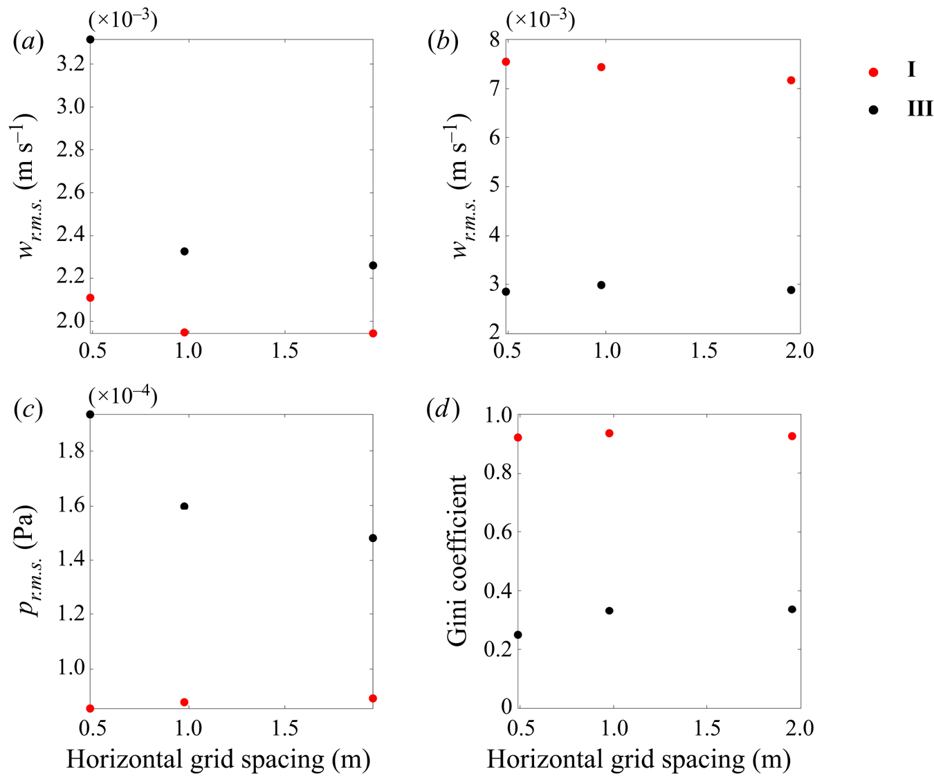
Figure 17. (a) Root-mean-square vertical velocity at  $z=-1$ m, (b) r.m.s. vertical velocity at $z=-30$ m, (c) r.m.s. pressure at $z=-1$ m, (d) Gini coefficient at $z=0$ m.
In case III, increasing the resolution causes a significant increase in the r.m.s. vertical velocity and r.m.s. pressure. Our simulations do not have sufficiently high resolution to capture all turbulent motions that develop close to the boundary at  $z=0$. For example, near-wall streaks develop in shear-driven turbulent boundary layers with a characteristic wavelength of $\lambda \simeq 100u^*/\nu$ (Smith & Metzler Reference Smith and Metzler1983). For $u^*=0.01$ m s $^{-1}$ and $\nu =10^{-6}\ \mbox {m}^2\ \mbox {s}^{-1}$, this gives $\lambda \simeq 1$ cm that is far too small to be resolved with our 1 m grid spacing. As the resolution is increased, we anticipate that more of the near-wall turbulent structures will be resolved in the simulations. Here however, we are interested in accumulation at a much larger scale (in § 3.3 we quantify clustering on a 31.25 m scale).
Figure 17(b) shows the dependence of the r.m.s. vertical velocity at  $z=-30$ m. In both cases I and III, the r.m.s. vertical velocity is weakly dependent on grid spacing. This is because the additional small-scale structures that feature under wind forcing only occur near the surface.
The random displacement model that we add to the particle motion equations helps compensate for the unresolved wind-driven turbulence. In § 3.3 we introduce the Gini coefficient to quantify particle clustering and we use the same quantity to check particle convergence, which can be seen in figure 17(d). In the case of the highest resolution, our domain size is reduced to 250 m and for a comparable particle distribution, we tile four 250 m domains together in a  $500\ {\rm m} \times 500$ m square with 1000 particles on each tile. We find that in case I the Gini coefficient is insensitive to grid spacing. In case III the Gini coefficient decreases by 26 % for the highest resolution. This is due to either missing larger-scale flow structures that are not present in the smaller domain size or additional small-scale structures that are resolved only on the highest resolution grid.
Appendix B
The 2-D Okubo parameter,  $Q$, is defined as
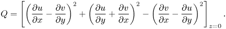 \begin{equation} Q = \left[\left( \frac{\partial u}{\partial x}-\frac{\partial v}{\partial y}\right)^2 + \left(\frac{\partial u}{\partial y}+\frac{\partial v}{\partial x}\right)^2 - \left(\frac{\partial v}{\partial x}-\frac{\partial u}{\partial y}\right)^2 \right]_{z=0}. \end{equation}
Regions with  $Q>0$ tend to be strain dominated, whilst regions with $Q<0$ can be understood as being vorticity dominated. Chor et al. (Reference Chor, Yang, Meneveau and Chamecki2018a) identified convective vortices as regions with extreme negative $Q$. Figure 18 shows the joint PDF of the Okubo parameter and pressure. In all cases, points with the most negative values of the Okubo parameter also have negative pressure. Under strong wind forcing, there are some points (figure 18b,c) that have negative pressure but a near-zero Okubo parameter. These may characterise horizontal vortices that form under wind shear and are not classified as vortices by the 2-D Okubo parameter.
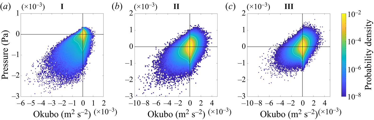
Figure 18. Joint PDF of the Okubo parameter at  $z=0$ m and pressure perturbation ( $\delta p$) at $z=-1$ m. White contours show where the PDF is $10^{-2}$ and $10^{-4}$.


 Open access