


1. Introduction
With high-speed large-capacity supercomputing facilities, numerical simulation has become an important practical tool to investigate geophysical or engineering problems involving snow deformation (Reference Bartelt and LehningBartelt and Lehning, 2002; Reference SchneebeliSchneebeli, 2004; Reference Johnson and HopkinsJohnson and Hopkins, 2005). Recently, snow mechanics has been applied to the high-fidelity numerical simulation of tire–snow interaction (Reference ShoopShoop, 2001; Reference LeeLee, 2009a). However, to obtain reliable results from numerical simulations requires suitable constitutive laws for snow, for the specific problem at hand (small and large deformations, low and high loading rates). This is a challenging task because the macroscopic mechanical behavior depends on the snow microscopic characteristics and other parameters such as temperature and free water content (Reference JohnsonJohnson, 1998; Reference Johnson and HopkinsJohnson and Hopkins, 2005). A comprehensive review of snow mechanics (Reference Shapiro, Johnson, Sturm and BlaisdellShapiro and others, 1997) has pointed out the need to establish an effective snow classification scheme using parameters that reflect microscopic information on snow such that specific macroscopic stress–strain relationships can be ascertained as a function of snow microstructure. Earlier attempts to solve this problem have suffered from the lack of an experimentally based technique to define and measure snow microstructure that allows a correlation to the thermal (Reference Kaempfer, Schneebeli and SokratovKaempfer and others, 2005) and macroscopic mechanical properties (Reference BrownBrown, 1980; Reference Mahajan and BrownMahajan and Brown, 1993; Reference Bartelt and LehningBartelt and Lehning, 2002; Reference SchneebeliSchneebeli, 2004) of snow; additional information can be found using the references cited in this paper.
The microstructural parameters (grain size, bond size, etc.) are generally measured as average values. As a naturally occurring material, snow’s microstructure, however, is formed in a stochastic rather than a deterministic sense. Snow then can be regarded as a random porous material, meaning that snow microstructure can also be characterized using statistical descriptors (e.g. two-point correlation function, lineal-path correlation function) to be elaborated in detail below. The effective physical properties of such a random material are determined by the statistical information embedded in the microstructure. The structure–property relationship for snows has been studied in the past. For example, by assuming the similarity of microstructures between snows and foams, mechanical properties of snows (e.g. Young’s modulus) have been modeled based on open-and closed-cell foams (Reference Kirchner, Michot, Narita and SuzukiKirchner and others, 2001; Reference PetrovicPetrovic, 2003). The elastic moduli are the simplest mechanical properties for solids, and hence are studied in this paper for the purpose of evaluating the quality of reconstructed microstructure. Analytical prediction of the upper and lower bounds of the effective elastic moduli of multiphase materials has long been the subject of many theoretical studies (Reference Hashin and ShtrikmanHashin and Shtrikman, 1963; Reference HillHill, 1965; Reference Roberts and GarbocziRoberts and Garboczi, 1999; Reference TorquatoTorquato, 2001); for example, the well-known Hashin–Shtrikman bounds on elastic moduli (Reference Hashin and ShtrikmanHashin and Shtrikman, 1963) were obtained knowing only the phase moduli and volume fractions of the material. However, volume fraction is not the only factor determining effective properties. For snow, for example, grain bonds play an important role in determining snow mechanical behaviors (Reference Bartelt and LehningBartelt and Lehning, 2002; Reference NicotNicot, 2004; Reference Johnson and HopkinsJohnson and Hopkins, 2005). The bounds can be improved by incorporating higher-order correlation functions of the microstructure such that effective properties can be predicted more precisely. On the other hand, large-scale computational methods have proved to be useful in determining composite material properties or behaviors given three-dimensional (3-D) geometric descriptions of the microstructures (Reference Garboczi and DayGarboczi and Day, 1995; Reference Roberts and GarbocziRoberts and Garboczi, 1999; Reference Johnson and HopkinsJohnson and Hopkins, 2005). Computational methods can yield direct relationships between the macroscopic properties and the microstructures of multiphase materials, which can provide comparison to analytical bounds and experimental results. More importantly, numerical methods, once validated, can provide an alternative method to establish microstructure–property relationships when experimental data are scarce.
The long-term goal of our research program is to establish a classification criterion of the mechanical behavior of snow based on the microstructural statistical information by carrying out large-scale numerical simulations, and compare the results with available experimental data. For microstructure-based numerical analysis, obtaining quantitative geometric representations of snow microstructure is the first step. Recently, X-ray microtomography (XMT) has been utilized to obtain 3-D high-resolution voxel-based images of snow microstructure (Reference Coléou, Lesaffre, Brzoska, Ludwig and BollerColéou and others, 2001). Experimental methods can be used to obtain real snow microstructure, but conducting the experiments can be demanding. If one can develop a stochastic model of the snow using the microstructural statistics of experimental data as input, it is hoped that one can reduce the number of tests and can obtain microstructure–property relationships using the stochastic model instead. Two-dimensional (2-D) surface micrographs are relatively easy to obtain experimentally. For a statistically isotropic and homogeneous porous material, the porosity and the two-point correlation function calculated from a 2-D image or a 3-D microstructure are the same. Therefore, 3-D microstructure can be numerically simulated by stochastic reconstruction techniques based on the statistical information obtained from 2-D images.
In this paper, the stochastic reconstruction of the snow microstructure and the calculation of effective elastic properties (Young’s modulus and Poisson’s ratio) are presented. The remainder of this paper is organized as follows. In section 2.1, we review the two widely used stochastic reconstruction methods and introduce in more detail the one chosen for the present study. In section 2.2, we summarize the various quantitative morphological measures that are frequently used in stochastic reconstruction to serve either as target functions or for comparison between the real and simulated microstructures. In section 2.3, we give a brief introduction of the material point method used to simulate the stress and strain fields of representative volume elements (RVEs), and the method of evaluating the effective elastic properties from these fields. In section 3, we describe the acquisition and processing of the real snow microstructure images obtained from XMT. In section 4, we present the results of simulated snow obtained from the stochastic reconstruction and compare them with those of real snow. The conclusion is presented in section 5.
2. Review of Theory
2.1. Stochastic reconstruction
When snow is considered as a random porous material, its microscopic morphology can be described by a two-valued random field Z(x), which is also referred to as the phase function:
where x is the 3-D space vector. The first and second statistical moments of the random field Z(x) are given as
where u is a lag vector and angle brackets denote statistical averages. In this paper, we only consider statistically isotropic and homogeneous porous materials, so p represents the porosity of the porous material, and the correlation function g 2, which can be written as g 2(u) (u = ||u||), is only a function of the length of u and is called the two-point correlation function. The two-point correlation function measures the probability that two points a distance u apart lie in the pore space. For random media without long-range order, it can be proved from Equations (1–3) that g 2(0) = p, g 2(∞) = p 2. The two-point correlation function of the solid phase is completely determined by the porosity, and the two-point correlation function of the pore phase by
where
![]() denotes the two-point correlation function of the solid phase. Therefore, if the two-point correlation function of the pore phase is reproduced in the stochastic reconstruction, that of the solid phase is also reproduced automatically. Moreover, for the reconstruction, only one of them needs to be used as the target information, i.e. the two-point correlation function cannot distinguish between the two phases.
denotes the two-point correlation function of the solid phase. Therefore, if the two-point correlation function of the pore phase is reproduced in the stochastic reconstruction, that of the solid phase is also reproduced automatically. Moreover, for the reconstruction, only one of them needs to be used as the target information, i.e. the two-point correlation function cannot distinguish between the two phases.
The purpose of the stochastic reconstruction is to numerically generate realizations of a two-valued random field Z′(x) that share the same statistical information (e.g. the porosity and the two-point correlation function) with the real microstructure Z(x). The original motivation for developing stochastic reconstruction methods is that 3-D microstructure of certain materials might be difficult or impossible to obtain experimentally. However, for these materials, 2-D surface micrographs might be readily acquired by conventional microscopy. For a statistically isotropic and homogeneous porous material, certain types of statistical information defined for 2-D surface images are the same as those defined in 3-D space; 3-D microstructure thus can be numerically simulated by stochastic reconstruction techniques based on the statistical information obtained from 2-D images.
Two major algorithms have been developed for the stochastic reconstruction of random media: the Gaussian random field (GRF)-based method (Reference QuiblierQuiblier, 1984) and the simulated annealing method (Reference Yeong and TorquatoYeong and Torquato, 1998). The GRF-based method is well studied, computationally efficient, but can only reproduce the porosity and the two-point correlation function of random porous materials. Therefore, it cannot ensure that the higher-order statistical information of the simulated random field is the same as that of the real microstructure. In contrast, the simulated annealing method can include as many statistical constraints as required in the objective function. But as the objective function becomes more complex, the convergence to reach a global minimum is also more difficult to achieve, and much higher computational cost is required.
Because of its high efficiency and robustness (Reference Quintanilla, Chen, Reidy and AllenQuintanilla and others, 2007), the GRF-based stochastic reconstruction technique was chosen in this study. Studies of this technique date back to 1974 (Reference JoshiJoshi, 1974). Based on Joshi’s work, Reference QuiblierQuiblier (1984) developed the 3-D stochastic reconstruction method which has been utilized in many practical problems to provide 3-D microscopic geometric descriptions. These fictitious 3-D microstructures were used to calculate the effective macroscopic properties of random porous or two-phase materials (Reference Adler, Jacquin and QuiblierAdler and others, 1990; Reference Kikkinides, Stefanopoulos, Steriotis, Mitropoulos, Kanellopoulos and TreimerKikkinides and others, 2002). Reference Roberts and TeubnerRoberts and Teubner (1995) and Reference RobertsRoberts (1997) brought this GRF-based stochastic reconstruction method into a general scheme, which can be briefly described as follows.
Let Y(x) denote a real-valued stationary isotropic Gaussian random field that is completely determined by its first and second statistical moments. For simplicity, assume 〈Y(x)〉 ≡ 0 and 〈Y(x) · Y(x)〉 = 1. Many numerical methods have been developed for the generation of realizations of a stationary GRF with a given correlation function gY (u) = 〈Y(x) · Y(x + u)〉. Therefore, the two-valued random field Z′(x) can be simply derived from Y(x) using the following one-level-cut procedure:
where α is the one-level-cut parameter. The porosity and the two-point correlation function of Z′(x) are denoted by p′ = (Z′(x)) and
![]() , respectively. Thus the remaining task is to ensure that p′ = p and
, respectively. Thus the remaining task is to ensure that p′ = p and
![]() . Since Z′(x) is associated with Y(x) by Equation (4), there exist relationships between p′,
. Since Z′(x) is associated with Y(x) by Equation (4), there exist relationships between p′,
![]() and α, gY
(u) (Reference TeubnerTeubner, 1991):
and α, gY
(u) (Reference TeubnerTeubner, 1991):
The statistical reconstruction method adopted in the present study consists of the following steps:
-
1. p′ and
 are directly given or computed from 2-D digital images of microstructure,
 -
2. gY (u) and α are computed from p′ and
using Equations (5) and (6), -
3. with gY (u) known, realizations of GRF Y(x) are numerically generated using the fast Fourier transform (FFT) method that is briefly described below,
-
4. with the one-level-cut parameter α, realizations of Z′(x) are generated using Equation (4).
By introducing the one-level-cut process, the original task of generating realizations of two-valued random field Z′(x) is then converted into generating realizations of GRF Y(x) with the correlation function gY (u). An evaluation and comparison of some GRF generators can be found in Reference FentonFenton (1994). In the present study, the FFT method was adopted to generate realizations of a GRF, as it is efficient and easy to implement. The discrete realizations of the random field Y(x) in a cubic domain V = L 3 are generated by the 3-D inverse FFT:
where h is the sample interval in each direction in the space domain V, and N = L/h is the number of sampling points in each direction. Here
![]() are random numbers given by
are random numbers given by
where
![]() and
and
![]() are independent Gaussian distributed random variables with zero mean and variance of one, and
are independent Gaussian distributed random variables with zero mean and variance of one, and
is the power spectral density function of the random field Y(x) (Reference TorquatoTorquato, 2001). It is worth noting that random fields generated by the FFT method automatically possess periodic boundary conditions which are required for statically homogeneous random fields in the sense that the random field is infinitely large.
2.2. Quantitative measures
Besides the porosity and the two-point correlation function, there are many other statistical measures that are briefly discussed below. Even though they are not used in the present statistical reconstruction, they can be utilized to evaluate the quality of reconstructed microstructure.
2.2.1. Specific surface area
Specific surface area s is defined as the ratio between the inner surface area of a snow sample and its volume. It is indicative of how well the area of the void–solid interface is reproduced. It was shown that the specific surface area for digitized media is a derived quantity of the discrete two-point correlation function g 2(u) (Reference Yeong and TorquatoYeong and Torquato, 1998):
where D is the space dimension. This equation implies that the accuracy of reproducing the specific surface area is closely related to how well the beginning part of the two-point correlation function is reproduced.
2.2.2. Correlation length
The correlation length of the pore space is related to the porosity and the two-point correlation function by (Reference Talukdar and TorsaeterTalukdar and Torsaeter, 2002)
Two points with a distance larger than the correlation length are regarded as having no correlation of the value of the phase function and being purely random to each other.
2.2.3. Lineal path function
The lineal path function of each phase, defined as Li (u) for statistically isotropic and homogeneous porous materials, is an important morphological quantity that measures the probability of finding a line segment of length u that lies entirely in the ith phase. Unlike the two-point correlation function, the lineal path functions of the pore phase and the solid phase are not simply related to each other. Moreover, this function contains some connectedness information that makes it a primary target function in the simulated annealing method (Reference Yeong and TorquatoYeong and Torquato, 1998).
2.2.4. Chord distribution function
Chord distribution function of each phase ci (u) is another useful characteristic related to chord length. The quantity ci (u) du is defined as the probability that a randomly picked line segment lying entirely in phase i has length in the range from u to u + du. This quantity directly gives the information about the connectedness and correlation of microstructure.
2.2.5. Local porosity distribution
The local porosity distribution μ(p, L) provides a characteristic length scale for determining the size of the RVE. The quantity μ(p, L) dp is the probability that the porosity of a randomly chosen cube of side length L falls into the range (p, p + dp).
2.2.6. Pore-size distribution function
The pore-size distribution function P(r), also referred to as pore-size probability density function, is defined such that P(r) dr represents the probability that a randomly picked point in the pore phase lies at a distance between r and r + dr from the nearest point on the pore–solid interface (Reference TorquatoTorquato, 2001). This function is an intrinsically 3-D microstructural measure and can only be obtained from 3-D samples. Note that if we consider pore phase as one of the two phases, the solid-size distribution function can be defined in the same way as the pore-size distribution function. The algorithm in Reference Bhattacharya and GubbinsBhattacharya and Gubbins (2006) is used in this paper.
2.3. Effective elastic properties
In addition to the comparison of quantitative geometric measures discussed above, we assess the quality of reconstructed snow by comparing the effective elastic properties of reconstructed snow with those of real snow via numerical modeling using the material point method (MPM; Reference Sulsky, Chen and SchreyerSulsky and others, 1994). MPM is one of the meshfree methods that utilize a background mesh as a computational scratch pad. We used the MPM component of the program Uintah, developed at the University of Utah (Reference Parker, Guilkey and HarmanParker and others, 2006), mainly due to its parallel capability and the ease of discretizing XMT images into material points (Reference Guilkey, Hoying and WeissGuilkey and others, 2006). In this paper, each voxel is mapped into a material point. The total number of material points for a typical microstructure is on the order of 50 × 106. A second incentive for using Uintah is to address the more challenging problem of calculating effective visco-plastic properties of snow from XMT images (Reference LeeLee, 2009b). Like many numerical methods, MPM can use the explicit and implicit algorithms; for this paper, we used the implicit algorithm (Reference Guilkey and WeissGuilkey and Weiss, 2003). Unconfined compression simulation was used to obtain the effective elastic properties; the displacement was prescribed on one side of the cube, and the reaction force was calculated. Effective stress was then calculated by dividing the reaction force by the cross-sectional area; the effective strain was obtained by dividing the displacement by the side length of the snow model. The effective Young’s modulus was then calculated by dividing the effective stress by the effective strain. For Poisson’s ratio, the average change of the snow model in the lateral direction was first calculated then divided by the side length of the snow model. To obtain statistics of the effective elastic properties, we used the stochastic reconstruction method discussed in this paper to generate five realizations (snow geometries) for reconstructed snow; for real snow, we sampled different parts of the snow to obtain five realizations.
We used two theories to put the results obtained from MPM in perspective. The first is the Hashin–Shtrikman upper-bound bulk modulus K U and shear modulus G U (Reference Hashin and ShtrikmanHashin and Shtrikman, 1963):
where p is the porosity or the volume fraction of air, and G and K are the shear and bulk modulus of ice, respectively. The second theory we used is for an open-cell foam (Reference Gibson and AshbyGibson and Ashby, 1997):
where E is Young’s modulus, ρ is density and v is Poisson’s ratio. We assume E ice = 9.3 GPa and v ice = 0.3 (Reference Petrenko and WhitworthPetrenko and Whitworth, 1999).
3. Analysis of X-Ray Microtomography Images
The snow sample was collected from the Agricultural Field at the University of Alaska Fairbanks, and subsequently sieved into different grain sizes. The smallest grain-size snow (<1 mm) was used in this study. Snow samples were put in a custom-made plastic container with a 1 cm diameter. The plastic container was mounted on the stage of an XMT scanner (SkyScan 1172 microtomograph) located in a cold room at −15°C. The scanning duration was from a few minutes to about half an hour, depending on acquisition settings. The exposure time was tuned to prevent snow samples from melting during the course of scanning. A collection of X-ray projection profiles was obtained from the scanner for the cylindrical-shaped snow sample. A series of cross-sectional images were then computed using reconstruction software NRecon. A cross-sectional image of the snow sample is given in Figure 1a. The cross-sectional images were further segmented into binary (black and white) images by computing a histogram of the gray values. Owing to the distinct brightness contrast of the images, the histograms of the images were found to be bimodal (inset in Fig. 1a). Accordingly, the gray value of the valley between two peaks was selected as the segmentation threshold. As shown in Figure 1b, isolated ice phase and pore phase appeared in the segmented images, induced by experimental noise or error of computer reconstruction process; the isolated pixels were removed using CTAn software. The binary counterpart of Figure 1a is shown in Figure 1c, where black pixels represent ice and white pixels denote pore. A 3-D visualization of a cube of the snow sample 3.618 × 3.618 × 3.618 mm3 in size is given in Figure 1d, where shaded area represents ice phase.
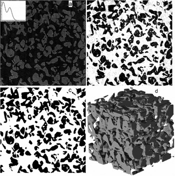
Fig. 1. (a) A gray-level cross-sectional image of the sieved snow sample; image size is 7.35 × 7.35 mm2 (pixel size 6 × 6 μm2). (b) The binarized counterpart of (a); small dots of pore and solid phase are artifacts due to the error of the scanning process and reconstruction process. (c) The result of removal of artifacts in (b). (d) 3-D visualization of a cube of snow microstructure, side length 3.618 mm.
The present study is only concerned with statistically isotropic and homogeneous porous materials. Therefore, the statistical average of the random field is identical to the ensemble average. The porosity of the snow sample was computed from the binary images to be 0.585, implying a snow density of 0.381 g cm−3 given the ice density of 0.917 g cm−3. The density was also directly estimated by measuring the mass and volume of the snow sample in order to verify the quality of the scanned images and the segmentation procedure. The measured density of the snow sample, 0.377 g cm−3, is in good agreement with 0.381 g cm−3. The two-point correlation function g 2(u) of a cross-sectional image can be computed using Equation (3) by interpreting the angle bracket as the ensemble average. The two-point correlation function of the snow sample (Fig. 2) depicts the autocorrelation of the microstructure as a function of the lag distance. At zero lag distance, the function is equal to the porosity p. At large lag distance, the function approaches its long-range value of p 2. The statistical isotropy of the snow microstructure is reflected in Figure 2, in which the two-point correlation functions in three orthogonal directions were found to be almost the same. The correlation length computed using Equation (12) is 56.2 μm. The porosity and the two-point correlation function given in Figure 2 from the real snow sample are the only input statistical information used for the stochastic reconstruction in the present study.
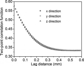
Fig. 2. Two-point correlation functions of the real snow sample in three orthogonal directions. Their consistency implies the statistical isotropy of the sample.
4. Results
With the porosity p and the two-point correlation g 2(u) of the real snow sample known, the one-level-cut parameter a and the correlation function gY (u), which are required to generate realizations of the random field, can be obtained by Equations (5) and (6). In the present study, the FFT method was used to numerically generate realizations of the GRF with the given correlation function. The realizations of the two-valued random field Z′(x) with desired statistical information were readily obtained through the one-levelcut procedure defined by Equation (4).
4.1. Two-dimensional reconstruction results
Equations (7–10) are written for 3-D cases. Replacing them with their counterparts for 2-D cases in the reconstruction procedure gives rise to the 2-D statistical reconstruction. Two-dimensional stochastic reconstruction can generate much larger images than 3-D reconstruction, computer memory for which is limited. For this reason, large 2-D images were reconstructed for visual evaluation of the reconstruction quality prior to 3-D reconstruction. The simulated 2-D microstructure is given in Figure 3. The only difference between Figure 3a and Figure 3b is that a high-frequency filter is used in Figure 3b to smooth the pore–solid interface. The threshold of the frequency filter is appropriately tuned such that the porosity change is <1%. Visual comparison between Figures 3b and 1c indicates that the microstructural morphologies of the simulated and actual images are quite similar. A quantitative comparison between the simulated snow and the real snow sample is presented in section 4.2.
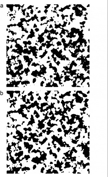
Fig. 3. The simulated 2-D microstructure; image size is 7.35 × 7.35 mm2 (pixel size 6 × 6 μm2). (a) Without high-frequency filtering. (b) High-frequency components filtered out to make the pore–solid interface smoother.
4.2. Three-dimensional reconstruction results
The 3-D reconstruction samples consist of 512 × 512 × 512 voxels (voxel size 12 × 12 × 12 mm3). The two-point correlation function of the 3-D simulated microstructure is plotted in Figure 4. It can be seen that the two-point correlation function of the simulated snow matches that of the real snow very well. It is worth noting that the GRF-based reconstruction method is a direct method, whereas the simulated annealing method is an iterative method. Thus, from the algorithmic point of view, the two-point correlation function is precisely reproduced in the GRF-based reconstruction procedure. In practical simulations, simulated finite domain size and domain discretization can result in slight error. The limitation of the GRF-based method is that it cannot ensure that the simulated microstructure has the same higher-order statistical information as the real microstructure.
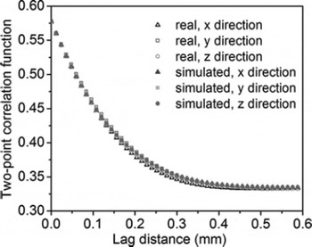
Fig. 4. The two-point correlation function of real and simulated snow. The two-point correlation function of the simulated snow matches well with that of the real snow.
To assess how well the other statistical information is reproduced, quantitative microstructure descriptors defined in section 2.2 were computed to evaluate the reconstruction quality. The specific surface area and correlation length are listed in Table 1. The reconstructed snow has a slightly higher specific surface area and correlation length than the real snow.
Table 1. Summary of reconstruction results (512 × 512 × 512 voxels)
The comparison of the lineal path functions is given in Figure 5a and b. It is important to stress that the lineal path function is reasonably well reproduced even though it is not used in the reconstruction. A similar conclusion was made in a study of the reconstruction of chalk pore networks using the simulated annealing method (Reference Talukdar and TorsaeterTalukdar and Torsaeter, 2002) where it was found that imposing the lineal path function as the target function in addition to the two-point correlation function only improves the reconstruction quality slightly. The drawback of the GRF-based reconstruction is that it only reproduces the first- and second-order statistical information. However, if the medium to be reconstructed is close to the Gaussian distribution, then no higher statistical information is needed and reasonable accuracy can be expected. Figure 5a, however, does show that the solid-phase lineal path function is slightly higher for the reconstructed than for the real snow, indicating that the solid phase of the reconstructed snow is more connected than that of the real snow. This also implies that the pore phase of the reconstructed snow is less connected than that of the real snow, as shown in Figure 5b. We attribute this discrepancy to the nature of the Gaussian distribution and the absence of higher statistical information as inputs. Incorporation of other statistical information will be attempted in future work.
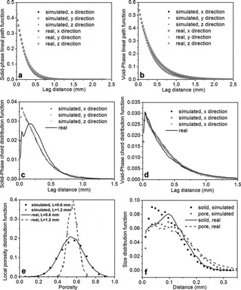
Fig. 5. Quantitative comparisons of the microstructure descriptors: (a) solid-phase lineal path functions; (b) void-phase lineal path functions; (c) solid-phase chord distribution functions; (d) void-phase chord distribution functions; (e) local porosity distribution functions; and (f) pore-size and solid-size distribution functions.
A reasonable match between simulated and real snow was also found for the other functions shown in Figure 5c–f. The void-phase chord distribution function is well reproduced as shown in Figure 5d. However, the peaks of the solid-phase chord distributions shown in Figure 5c vary significantly, indicating there are more single-voxel solid-phase chords for the reconstructed snow.
The local porosity distribution functions and the size distribution functions are compared in Figure 5e and f, respectively. The solid and pore-size distribution functions (Fig. 5f) are similar to the solid- and void-phase chord distribution functions. A 3-D visualization of a cube of the simulated sample 3.84 × 3.84 × 3.84 mm3 in size is shown in Figure 6 where shaded area represents the solid phase.
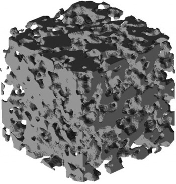
Fig. 6. 3-D visualization of the simulated snow microstructure (3.84 × 3.84 × 3.84 mm3).
4.3. Results of elastic moduli
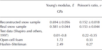
Figure 7 shows the comparison of Young’s moduli and Poisson’s ratios (in means and standard deviations) for real and reconstructed snow as a function of the size of the snow cube using MPM simulations. For the largest real snow of 7.488 mm side length, only one sample is available, so no statistics can be obtained. For real snow, the Young’s modulus remains almost constant, but increases slightly with side length. For reconstructed snow, no trend can be observed. Table 2 shows that the reconstructed snow has a higher Young’s modulus than the real snow; this is attributed to the higher connectedness of the solid phase of the reconstructed snow (cf. Fig. 5a, c and f). The Young’s moduli for both real and reconstructed snows are at the higher end of the test data, probably because the snow used in this paper is sieved and more uniform. Since ice creeps easily, it is difficult to measure the Young’s modulus of snow accurately by isolating the viscous effect (Reference Kirchner, Michot, Narita and SuzukiKirchner and others, 2001), i.e. some test results of Young’s modulus reported in the literature could be a tangent modulus which is smaller than the intrinsic Young’s modulus, such as calculated in this paper, where viscous effect is absent in the constitutive model; our approach is similar to that of Reference SchneebeliSchneebeli (2004) where the order of magnitude of Young’s modulus calculated is similar to ours. The Young’s moduli from simulations are all much smaller than those due to the open-cell foam model or the theoretical Hashin–Shtrikman bound; the moduli from open-cell foam can thus be considered a better upper bound than the Hashin–Shtrikman bound for the snow studied. The Poisson’s ratios are all smaller than those from the test data and theories. It is known that Poisson’s ratio is more difficult to ascertain for a porous than for a solid material (Reference Gibson and AshbyGibson and Ashby, 1997); this aspect needs further investigation. Although it is difficult to draw a definitive conclusion regarding the size of the RVE for the snow being studied, 5–6 mm seems to be a reasonable range judging from the distribution of Young’s moduli in Figure 7.
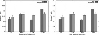
Fig. 7. Means and standard deviations of elastic moduli (a) and Poisson’s ratios (b) of simulated and real snow as a function of the side length of the snow.
Table 2. Summary of elastic moduli from simulations and theories
5. Conclusions
Obtaining a quantitative geometric description of snow microstructure is essential to investigations of microstructure-based mechanical or thermal behaviors of snow. Despite recent advances in experimental methods (e.g. XMT), stochastic reconstruction of snow microstructure based on statistical modeling, being a numerical method, can be an important alternative. The GRF-based stochastic reconstruction of the sieved and sintered dry-snow sample with grain size <1 mm has been investigated in the present study. The visual and quantitative comparisons between the simulated and real snow microstructure indicated that the stochastic reconstruction of this type of snow microstructure is reasonably accurate even though only the porosity and the two-point correlation function were used. The nature of Gaussian distribution and the absence of higher statistical information as inputs may lead to the higher connectedness in the simulated than in the real microstructure. The drawback of the GRF-based reconstruction is that it only reproduces first- and second-order statistical information. However, if the medium to be reconstructed is close to the Gaussian distribution, then higher statistical information is not needed and reasonable accuracy can be expected. In conclusion, the GRF-based stochastic reconstruction technique is reasonably accurate, robust and highly efficient in numerical simulations, making it a promising algorithm for providing 3-D quantitative geometric descriptions of random porous materials.
The preliminary computations of the effective elastic moduli of varying sizes of RVEs demonstrated the potential of the stochastic modeling of snow microstructure for investigating the microstructure–property relationship. Further work is needed to determine this relationship by obtaining improved statistical information for the stochastic reconstruction beyond the porosity and the two-point correlation function.
Acknowledgements
We thank H. Löwe for helpful comments on the manuscript. This work was supported in part by a grant of high-performance computing resources from the Arctic Region Supercomputing Center at the University of Alaska Fairbanks as part of the US Department of Defense High Performance Computing Modernization Program. J.H. Lee and H. Yuan gratefully acknowledge financial support from the Automotive Research Center (ARC), a US Army Research, Development and Engineering Command (RDECOM) Center of Excellence for Modeling and Simulation of Ground Vehicles led by the University of Michigan, and the support of the US Army Tank Automotive Research, Development and Engineering Center (TARDEC). J.E. Guilkey gratefully acknowledges financial support from DOE W-405-ENG-48 (Center for the Simulation of Accidental Fires and Explosions (C-SAFE), University of Utah).


