


Introduction
Sea urchins play a major role in marine benthic ecosystems and have significant ecological significance in shaping the structure of marine communities, among other functions (Uthicke et al., Reference Uthicke, Schaffelke and Byrne2009; Lawrence, Reference Lawrence2020). The study of growth and age is therefore crucial for understanding the life cycle and population dynamics of these key benthic organisms, while also providing valuable information to examine environmental effects (Clarke, Reference Clarke1991; Ebert, Reference Ebert and Lawrence2020). Specifically, sea urchin growth involves the incorporation of new plates into the endoskeleton and the enlargement of existing plates through the addition of calcite along their edges (Ellers et al., Reference Ellers, Johnson and Moberg1998; Johnson et al., Reference Johnson, Salyers, Alcorn, Ellers and Allen2013). Furthermore, sea urchins possess additional calcium carbonate structural components, including elements of Aristotle's lantern, which experience growth by incorporating calcite across their entire surface, with a stronger emphasis on the aboral end (Johnson et al., Reference Johnson, Salyers, Alcorn, Ellers and Allen2013).
In order to make inferences about growth in sea urchins, information on changes in body size with age is required, followed by growth modelling (Pecorino et al., Reference Pecorino, Lamare and Barker2012). The methods used to examine growth in sea urchins are varied and include cohort analysis using size structure data, analysis of growth lines, as well as tagging and recapture and cage culture experiments (Ebert, Reference Ebert and Lawrence2020; Tourón et al., Reference Tourón, Campos, Costas and Paredes2023). Growth modelling includes asymptotic models (e.g. Brody–Bertalanffy, Richards, logistic, Gompertz, and Jolicoeur) in addition to more complex models with continuous, non-asymptotic growth, such as the Tanaka model (Ebert and Russell, Reference Ebert and Russell1993).
Studies using fluorescent markers have found that growth lines in endoskeletal plates of some sea urchin species are not added annually, and therefore, they would not be good age estimators (Gage, Reference Gage1992; Russell and Meredith, Reference Russell and Meredith2000). Methods involving chemical tagging and recapture are most efficient and robust, and among them, the antibiotic tetracycline and calcein are the most widely used (Tourón et al., Reference Tourón, Campos, Costas and Paredes2023). These fluorochromes irreversibly bind to the calcium ions in the developing endoskeleton and have been shown not to interfere with the regular growth of tagged individuals (Ebert, Reference Ebert, Burke, Mladenov, Lambert and Parsley1988; Russell and Urbaniak, Reference Russell, Urbaniak, Heinzeller and Nebelsick2004; Ellers and Johnson, Reference Ellers and Johnson2009). Among these fluorochromes, calcein offers greater advantages due to its higher absorption and fluorescence, and lower toxicity, enabling tagging of sea urchins though coelomic injection or chemical immersion (Haag et al., Reference Haag, Russell, Hernández and Dollahon2013; Ebert, Reference Ebert and Lawrence2020).
The genus Pseudechinus comprises 11 species with a wide geographic distribution in temperate-cold waters of the Southern Hemisphere (Pierrat et al., Reference Pierrat, Saucède, Festeau and David2012; Kroh and Mooi, Reference Kroh and Mooi2023). Only a single species, Pseudechinus magellanicus (Philippi, 1857), is distributed in the southern tip of South America, ranging from Puerto Montt (~40°S) in the Pacific Ocean to Río de la Plata estuary (35–36°S) in the Atlantic Ocean, including Falklands/Malvinas and South Georgia Islands (Bernasconi, Reference Bernasconi1953; Pawson, Reference Pawson1966; Brogger et al., Reference Brogger, Gil, Rubilar, Martínez, Díaz de Vivar, Escolar, Epherra, Pérez, Tablado, Alvarado and Solís-Marín2013). It also occurred over a wide bathymetric range of 0–360 m (Larrain, Reference Larrain1975).
P. magellanicus is the most abundant sea urchin species in central and south Patagonia in Argentina and southern Chile and plays an important ecological role in trophic webs within coastal and nearshore benthic communities (Ríos et al., Reference Ríos, Mutschke and Cariceo2003; Penchaszadeh et al., Reference Penchaszadeh, Bigatti and Miloslavich2004; Zaixso et al., Reference Zaixso, Boraso, Pastor, Lizarralde, Dadon, Galván, Zaixso and Boraso2015; Gil et al., Reference Gil, Boraso, Lopretto and Zaixso2021). Due to its ubiquitousness in these austral ecosystems, some biological aspects have been explored (Marzinelli et al., Reference Marzinelli, Bigatti, Giménez and Penchaszadeh2006; Gil, Reference Gil2015; Détrée et al., Reference Détrée, Navarro, Font and Gonzalez2020, Reference Détrée, Navarro, Garrido, Bruning and Leclerc2023; Gil et al., Reference Gil, Lopretto and Zaixso2020). Although it is commonly referred to as a dwarf sea urchin, there is a lack of information regarding growth estimates for this species. To gain insights into the factors influencing population dynamics, studies are needed to evaluate the individual growth patterns. Thus, the main objective of this study was to assess the growth of P. magellanicus in central Patagonia (Argentina) using calcein-tagging techniques, providing the first growth assessment for this species in coastal habitats.
Materials and methods
Study area
The study was conducted on a wave-exposed rocky shore located in the central coast of San Jorge Gulf, Argentina (La Tranquera beach: 46°02′24.61″S; 67°35′52.61″W; Figure 1). The site is composed of relatively hard sedimentary bedrock and show large (~30–45 m2) and deep tidepools (approximately <3 m depth) located in the low mid-littoral zone and upper infralittoral fringe. Tidepool bottoms exhibit high structural complexity, characterized by bare rocky substrates with crevices and loose rocks, shells, and debris. These substrates can also be covered with various organisms, such as clumps of turfing coralline algae and mussel beds (Zaixso et al., Reference Zaixso, Boraso, Pastor, Lizarralde, Dadon, Galván, Zaixso and Boraso2015). Additionally, tidepools support abundant populations of P. magellanicus, and occasionally host typical species found in the subtidal or infralittoral shore zones, including juvenile king crabs, Lithodes santolla, or the sea star Cosmasterias lurida. These environments were specifically chosen against shallow tidepools in order to minimize environmental stress on the growth of sea urchins and favour retention of tagged sea urchins. Seawater temperatures in the region ranged annually between 6.1 and 13.0°C and salinity is ~34.5 (Verga et al., Reference Verga, Tolosano, Cazzaniga and Gil2020).

Figure 1. Study area for the tag and recapture experiment of P. magellanicus in central Patagonia, Argentina.
Tagging and recapture
Sea urchins were collected from tidepools using autonomous diving and snorkelling. Tidepool bottoms and Corallina officinalis turfs were carefully inspected for the presence of juveniles and small sea urchins during fieldwork. Upon collection, sea urchins were promptly transferred to 40 l containers and stored in shaded and cooled areas. Calcein, a fluorescent marker, was utilized for tagging the sea urchins. The calcein solution was prepared by adjusting the concentration to 500 ppm using filtered seawater (45 μm) and gradually adding NaOH to achieve a pH of 8. For sea urchins >15 mm in test diameter, calcein was incorporated through coelomic injection (0.3–0.9 ml) administered with caution via the peristomial membrane. In the case of smaller sea urchins (<15 mm), the fluorochrome was incorporated through osmotic absorption. This was accomplished by immersing the individuals in a concentrated solution of 500 ppm for 24 h. During fieldwork, this solution was kept refrigerated using ice-packs, and an aerator was used to ensure a continuous oxygen supply. Sea urchins were then transferred to a temperature-controlled refrigerator set between 7 and 10°C and released back into the study area the following day. This marking procedure was conducted on ~1100 individuals with a size range of 9–25 mm on 13 March 2008. After a period of 376 days (equivalent to 1.03 years), a total of 461 specimens from the same tidepool areas were recaptured and subsequently stored in a freezer at −30°C for further processing.
Growth readings
In the laboratory, the test diameter (D) of each individual was measured using a Vernier caliper (±0.01 mm) and individually placed in a solution of sodium hypochlorite (NaOCl; 55 g l−1) for at least 24 h to remove organic matter. The test and Aristotle's lantern were subsequently rinsed with tap water and carefully dried in a dark and ambient room for a period of 3–4 days. After the drying process, the length of a demi-pyramid, extending from the oral end to the junction with the epiphysis (as depicted in Figure 2a), was measured in accordance with the guidelines outlined by Lamare and Mladenov (Reference Lamare and Mladenov2000).

Figure 2. (a) Schematic measurements on demi-pyramid, where Lt +1 represents the sum of the length from the oral end to the union with the epiphysis at tagging (Lt), plus the increase after 1 year (ΔL). (b, c) Fluorescent calcein-tag visualization at the aboral end of P. magellanicus demi-pyramid. Arrows show the discrete calcein mark. Scale bar: 300 μm.
The presence of the calcein tag in the demi-pyramids was observed using an epifluorescence microscope equipped with Neofluar objectives, and a BP450–490 exciter filter, an FT510 chromatic beam splitter, and an LP520 barrier filter (Zeiss). Calcein, which binds to calcium carbonate, exhibits maximum excitation at 495 nm (range 470–500 nm) and emitting green light at 515 nm. Careful attention was given to distinguish the calcein fluorescence from the yellow autofluorescence produced by other organic and inorganic substances, ensuring that the calcein tag was clearly visible and easily recognizable due to its distinct green coloration.
Growth increments were assessed following established methods used in other sea urchin species (e.g. Russell, Reference Russell1987; Lamare and Mladenov, Reference Lamare and Mladenov2000; Ebert et al., Reference Ebert, Russell, Gamba and Bodnar2008). When a discrete and clear linear green mark was visible, following measurements (±0.01 mm) were taken: (1) total length of the demi-pyramid of the recaptured animal after 1 year (Lt +1), and (2) the increase in length (ΔL) at the aboral end of the demi-pyramid, representing the net growth of the demi-pyramid over 1 year. The difference between these measurements provided the length of the demi-pyramid at the time of marking (Lt) (Figure 2). Although demi-pyramid growth in sea urchins can occur at both ends, the oral end typically exhibits minimal growth, which may be insignificant compared to the aboral edge (Ebert et al., Reference Ebert, Russell, Gamba and Bodnar2008; Johnson et al., Reference Johnson, Salyers, Alcorn, Ellers and Allen2013). In the case of P. magellanicus, no observable net growth was observed at the oral end of the demi-pyramids due to the absence of a distinct mark.
Growth modelling
The relationship between demi-pyramid length (Lt) data and test diameters (Dt) was examined by fitting a model II non-linear regression with the below equation:

to facilitate the conversion between the two variables (Ebert and Russell, Reference Ebert and Russell1994). Parameters were estimated using the quasi-Newton optimization procedure.
To evaluate the growth rates of the calcein-marked individuals, Walford plots (Walford, Reference Walford1946) were utilized, wherein the test diameter at the time of marking (Dt) was plotted against the diameter at the time of recapture 1 year later (Dt +1). Subsequently, a regression analysis, employing either linear or non-linear regression models (see below), was performed to estimate the parameters of the Brody–Bertalanffy and Richards growth models (Ebert and Russell, Reference Ebert and Russell1993; Pecorino et al., Reference Pecorino, Lamare and Barker2012). The linear relationship observed between Dt +1 and Dt indicated the suitability of both the Brody–Bertalanffy and Richards growth models (Pederson and Johnson, Reference Pederson and Johnson2008).
Growth models, difference equations, and instantaneous growth rates equations were obtained from Lamare and Mladenov (Reference Lamare and Mladenov2000) and Ebert and Russell (Reference Ebert and Russell1993):
Brody–Bertalanffy growth model

The parameters of this function (D ∞ and k) were obtained using Walford plots and fitting the data to a linear regression model, Dt +1 = c + mDt. The slope of the regression was m = e−kt. Thus,


where t is the time elapsed between the initial and final measurements and the size at settlement D 0 was set at 0.4 mm (minimum size of recruits in the field; Gil, Reference Gil2015). The instantaneous growth rate for the model is given by

Lastly, due to the negative association between D ∞ and k in the estimated parameters of the Brody–Bertalanffy function, a growth index θ (Munro and Pauly, Reference Munro and Pauly1983) was calculated to enable comparisons with other sea urchin species.
Richards growth model

The parameters of this function were estimated using non-linear iterative procedures employing the quasi-Newton algorithm on the relationship between Dt +1 and Dt given by

Then,


The instantaneous growth rate for the Richards model is

Model selection
The proposed models were compared using the sum-of-squared errors and the corrected Akaike information criterion (AICc) (Burnham and Anderson, Reference Burnham and Anderson2002). The model with the lowest AIC value (maximum parsimony) was selected to ensure optimal complexity and goodness-of-fit.
All statistical analyses were performed using Statistica 13.0 for Windows (StatSoft Inc.). A significance level of 5% was used for all statistical analyses.
Results
Tagging and recapture efficiency
A total of 461 sea urchins were recaptured after 1 year. The size distribution of sea urchins at the time of recapture ranged 11.42–24.23 mm (mean: 17.67 mm [±2.17 SD]; n = 447) and showed a general unimodal pattern dominated by individuals with test diameters between 15 and 20 mm (Figure 3a). Fourteen recaptured sea urchins were excluded from the size distribution analysis as they exhibited broken tests.

Figure 3. (a) Size–frequency distribution of P. magellanicus in tidepool habitats of the San Jorge Gulf at the time of recapture. (b) Proportion of tagged sea urchins across size categories, with n indicated in parentheses.
Out of the total recaptured (n = 461), 48 individuals were identified with fluorescent-calcein tags in their demi-pyramids (10.4%). However, only 36 of these individuals had well-defined fluorescent lines (7.8% effective recapture) (Figure 2b and c). Although the recapture rate was relatively low, the absolute number of sea urchins with visible marks that were recaptured was considered sufficient for data analysis. Tagged sea urchins ranged 11–23 mm of test diameter and included the upper 60% segment of the size distribution. The recapture rate by size classes is shown in Figure 3b.
Growth analysis
Relationship between test diameter and demi-pyramid length
A model II power relationship was fitted between demi-pyramid length and test diameter of P. magellanicus (r 2 = 0.66; Figure 4a).
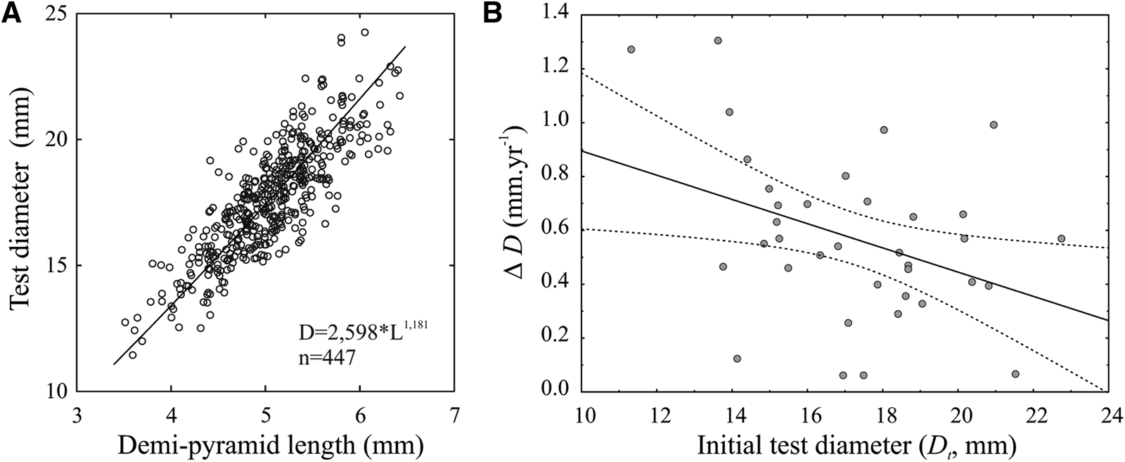
Figure 4. (a) Power regression (model II) between test diameter (D) and demi-pyramid length (L) in P. magellanicus. (b) Variation in individual growth (ΔD, mm year−1) of recaptured and tagged sea urchins. The solid line indicates a significant linear relationship (p < 0.05) (ΔD = 1.34–0.045Dt; r 2 = 0.17), and the dotted line represents the 95% confidence interval.
The analysis of individual growth rate (mm year−1) in relation to the initial size ranged between 0.05 and 1.3 mm year−1, with a significant negative linear relationship between the increase in diameter after 1 year (ΔD) and the initial size (Dt) (Figure 4b).
Growth modelling and model selection
The Walford plots revealed a linear relationship between the test diameter at the time of tagging (Dt) and after 1 year (Dt +1) for the range of recaptured sizes (Figure 5). These plots consistently showed slow growth within most of the studied size range. Particularly, individuals of P. magellanicus with a diameter exceeding 21 mm exhibited positive growth, albeit at a reduced rate, and did not approach zero growth (Figures 4 and 5).

Figure 5. Walford plots for the Brody–Bertalanffy and Richards growth models for P. magellanicus after 1 year period. Red line denotes the absence of growth.
Growth parameter estimates are summarized in Figure 6. The Brody–Bertalanffy growth model estimated a maximum asymptotic diameter of 29.89 mm, and the Richards model estimated it to be 26.01 mm. The growth constant (k) exhibited low and comparable values in both models. According to the Brody–Bertalanffy model, the maximum instantaneous growth rate was determined to be 1.36 mm year−1, whereas the Richards model predicted a maximum rate of 2.69 mm year−1. Both models indicate that maximum growth occurs at the recruitment age (Figure 6).

Figure 6. Growth curves (solid line) and instantaneous growth rates (dashed line; IGR) for the Brody–Bertalanffy and Richards growth models: D ∞: asymptotic diameter; k: growth constant; n: Richards shape parameter. MGR, maximum growth rate (mm year−1). Dotted lines represent D ∞ and D max as the maximum test diameter observed in the field.
The Brody–Bertalanffy growth model showed a better fit, indicated by lower values of the residual sum-of-squares and AICc (Table 1). However, the difference in AICc values was less than 4, indicating that both models were suitable (Burnham and Anderson, Reference Burnham and Anderson2002). After inspection of the relationship between the maximum diameter observed in the field (D max) and the estimated asymptotic maximum diameter, the Richards model showed a better approximation. Additionally, this model exhibited higher initial growth and a subsequent decline in growth rates at larger sizes compared to the Brody–Bertalanffy model (Figure 6).
Table 1. Selection of growth models for tagging and recapture data of P. magellanicus in central Patagonia, Argentina

Despite the slight variations observed among the competing models, P. magellanicus exhibited low asymptotic diameters and growth constants. The most common adult sizes (~16–20 mm; Figure 2) correspond to ages ranging from 15 to 21 years (inferred from the Brody–Bertalanffy model). Regarding the estimators obtained from the Brody–Bertalanffy growth model (k and D ∞), the growth index (θ) for the studied population was 3.72.
Discussion
This study presents the first assessment of somatic growth in the sea urchin P. magellanicus using calcein tagging in coastal populations from central Patagonia (Argentina). The recapture rate of tagged individuals was relatively low but considered sufficient based on established criteria in similar studies (e.g. Lamare and Mladenov, Reference Lamare and Mladenov2000; Kirby et al., Reference Kirby, Lamare and Barker2006). The low recapture rate could be attributed to various factors, including limited success in marking individuals in the field, high mortality of tagged individuals, and, to some extent, features of the tidepool environment where sea urchins were released after tagging. Calcein, being the least toxic among fluorescent markers, generally does not cause harmful effects in sea urchins (Rowley and Mackinnon, Reference Rowley and Mackinnon1995; Russell and Urbaniak, Reference Russell, Urbaniak, Heinzeller and Nebelsick2004, Lau et al., Reference Lau, Dumont, Lui and Qiu2011). The presence of a significant number of unmarked animals supports the hypothesis of significant mixing after the recapture period due to high population density in tidepool areas (max. 444 ind m−2, mean: 50.6 ind m−2; Gil, Reference Gil2015) and presence of large and deep tidepools. The cryptic behaviour exhibited by the species (Gil, Reference Gil2015) could also have influenced the recapture rates. Even though seasonal effects on calcification were not directly investigated in this study, tagging of P. magellanicus was conducted in late summer, a period when calcification has been observed in other temperate-cold water sea urchin species (Gage, Reference Gage1991). Kirby et al. (Reference Kirby, Lamare and Barker2006) attribute the low recapture rate of Pseudechinus huttoni to vertical migration phenomena, which is unlikely to have affected our experiments conducted within a relatively confined natural environment.
The validity of the obtained growth estimates for P. magellanicus may be partially limited due to the absence of very small-sized animals. This limitation could affect the shape of the growth curves in the lower size range (<11 mm) where growth estimators could not be validated. However, similar situations have been noted in Sterechinus neumayeri, where the addition of smaller specimens did not significantly alter the parameters of the growth function (Brey et al., Reference Brey, Pearse, Basch, McClintock and Slattery1995). Kirby et al. (Reference Kirby, Lamare and Barker2006) also encountered limitations in interpreting growth models for P. huttoni as their dataset only included larger individuals and lacked data on animals smaller than 20 mm in diameter. In other invertebrates, Haag (Reference Haag2009) suggests that growth estimators in tagged and recaptured species may be biased if a wide size range is not covered. Data solely representing the upper fraction of larger sizes would result in age overestimations, while focusing only on smaller sizes would lead to underestimations. In our case, the range of marked recaptured sizes ranged from 11 to 24 mm, encompassing ~60% of the upper size spectrum when considering a maximum field size of ~25 mm. Thus, although our age estimators may show some limitations, they are considered optimal.
As far as we know, P. magellanicus is the smallest sea urchin species in which growth has been investigated. It shows low growth constants and asymptotic diameters (Table S1). Although the Brody–Bertalanffy growth model provides a reasonable fit to our data, it is essential to consider certain limitations and potential biases associated with this model. Rogers-Bennett et al. (Reference Rogers-Bennett, Rogers, Bennett and Ebert2003) highlight that the annual growth rate for juveniles is often lower than what is typically predicted by the Brody–Bertalanffy model. In our study, we documented high growth rates among individuals of smaller sizes. Nonetheless, it is important to acknowledge that the absence of recaptured juvenile individuals poses a potential bias in the final growth model, as previously mentioned. The inclusion of juvenile data in mark–recapture studies of sea urchins is uncommon, with only a limited number of studies, including such data (e.g. related to Strongylocentrotus franciscanus), typically acquired through the collection and marking of juveniles in laboratory experiments (Ebert and Russell, Reference Ebert and Russell1993; Ebert et al., Reference Ebert, Dixon, Schroeter, Kalvass, Richmond, Bradbury and Woodby1999; Johnson et al., Reference Johnson, Salyers, Alcorn, Ellers and Allen2013). These studies revealed an initial growth delay, followed by exponential growth, and ultimately a gradual decrease in the growth rate in adult individuals. Nonetheless, it is important to note that not all sea urchins exhibit the same growth pattern, and significant variability exists among species (Ebert, Reference Ebert and Lawrence2020). Another aspect deserving consideration is the almost lack of asymptotic growth (i.e. ΔD approaching zero) in large individuals. This observation suggests that P. magellanicus exhibits either low and non-asymptotic growth within the range of the maximum sizes studied or a greater variability in the final sizes of adult individuals. Nevertheless, there is a discernible trend towards a reduction in the rate of growth in larger animals (as shown in Figure 5). Within this framework, the Tanaka model has been employed to account for indeterminate growth in sea urchins (Ebert et al., Reference Ebert, Dixon, Schroeter, Kalvass, Richmond, Bradbury and Woodby1999). This model exhibits a curvilinear relationship with up to two inflection points, as observed in Walford plots. However, the presence of a linear relationship in the Walford plots for P. magellanicus suggest the application of the Tanaka model unfeasible, thereby establishing the Brody–Bertalanffy and Richards models as more suitable alternatives (Ebert et al., Reference Ebert, Dixon, Schroeter, Kalvass, Richmond, Bradbury and Woodby1999; Lamare and Mladenov, Reference Lamare and Mladenov2000). Furthermore, the estimated asymptotic diameters are consistent with the maximum diameters found in the field and in other ecological studies (~28–30 mm; Ríos et al., Reference Ríos, Mutschke and Cariceo2003; Escolar, Reference Escolar2010; Gil, Reference Gil2015). Moreover, Mortensen (Reference Mortensen1910) report that the species can reach 40 mm off eastern Malvinas/Falkland Islands, a southern insular locality suggesting that growth estimates can vary spatially. In this context, Lamare and Mladenov (Reference Lamare and Mladenov2000) reported a similar situation for Evechinus chloroticus, wherein they found occurrences of non-asymptotic growth but ultimately determined that the asymptotic Richards model provided the best fit. To further explore the nature of asymptotic or indeterminate growth in P. magellanicus, further studies should involve recapturing individuals over a more extended period.
The growth constants (k) for the Brody–Bertalanffy growth model in other sea urchin species range from 0.011 to 1.80, while the asymptotic diameters (D ∞) vary between 29.9 and 152.1 mm (Table S1). Among the regular sea urchins studied so far, P. magellanicus exhibits the lowest asymptotic diameter and growth index (θ). The Antarctic sea urchin Sterechinus antarcticus exhibits a lower growth constant compared to P. magellanicus (Brey et al., Reference Brey, Pearse, Basch, McClintock and Slattery1995), but it attains a larger asymptotic diameter of up to 80 mm and can live for over 70 or 80 years (Brey, Reference Brey1991). Age estimates for P. magellanicus based on fitted models indicate maximum ages of ~40 years and first sexual maturity occurred, according to size at first maturity estimated by Orler (Reference Orler1992), in 7–9 years. The longevity of sea urchins is known to be variable, and its determination can also be influenced by the methodology employed. Age estimates obtained using plate rings in different species of regular sea urchins suggest lifespans ranging from 4 to 75 years (Ebert and Southon, Reference Ebert and Southon2003). However, caution is advised when interpreting ring bands, as natural bands often underestimate the age of large animals due to overlapping of light and dark lines in very small increments that are difficult to discern (Ebert, Reference Ebert, Burke, Mladenov, Lambert and Parsley1988; Ebert and Southon, Reference Ebert and Southon2003). In contrast, tag and recapture methods tend to provide somewhat higher and more consistent age estimates (Ebert and Southon, Reference Ebert and Southon2003). Moreover, tagging methods and radiocarbon dating across a wide size range found that S. franciscanus can live for over 100 years (Ebert and Southon, Reference Ebert and Southon2003). Strongylocentrotus droebachiensis also exhibits maximum lifespans exceeding 100 years (Russell et al., Reference Russell, Ebert and Petraitis1998). According to Kirby et al. (Reference Kirby, Lamare and Barker2006), the presence of a low growth rate and high longevity is commonly associated with deep-water species. However, some exceptions have been documented for shallow-water sea urchin populations such as Paracentrotus lividus or S. franciscanus (Ebert and Russell, Reference Ebert and Russell1993; Ebert and Southon, Reference Ebert and Southon2003; Ouréns et al., Reference Ouréns, Flores, Fernández and Freire2013).
Empirical evidence suggests that sea urchin growth often diverge between species or even populations (Table S1), and is known to be affected by different environmental (e.g. temperature) and ecological factors (e.g. food availability and density-dependent processes) (Ebert, Reference Ebert and Lawrence2020). Although growth estimates within the genus Pseudechinus are still poorly studied, the variability observed using the same methods (calcein tagging) compared with P. huttoni from New Zealand (Table S1; Kirby et al., Reference Kirby, Lamare and Barker2006) could be partially explained by different environmental contexts and evolutionary histories. P. huttoni was studied in deep fjords, a more stable and slightly warmer environment compared to wave-exposed rocky shores in central Patagonia, showing a higher growth constant (0.15–0.56) and reaching larger asymptotic sizes (33.8–42.7 mm) (Kirby et al., Reference Kirby, Lamare and Barker2006). This highlights the necessity to perform growth analysis in other populations and species within the genus. The low growth rate and reduced asymptotic size observed in P. magellanicus may provide an evolutionary advantage by facilitating its colonization of cryptic microhabitats, both in subtidal (e.g. holdfasts of Macrocystis pyrifera) and intertidal zones (e.g. in San Jorge Gulf) (Gil, Reference Gil2015). Evolutionary hypotheses propose that growing smaller under cold conditions offers disadvantages due to (1) increased mortality, (2) diminished fecundity, and (3) low resistance to starvation caused by limited resources (Verberk et al., Reference Verberk, Atkinson, Hoefnagel, Hirst, Horne and Siepel2021). However, although the ultimate explanations lie beyond the scope of this paper, the small body size exhibited by P. magellanicus could also be related to a low predation pressure and hence low mortality, and high predictability and availability of food in coastal ecosystems, primarily due to its dietary plasticity (Gil et al., Reference Gil, Boraso, Lopretto and Zaixso2021). Within the coastal ecosystems of Patagonia and southern Chile, the presence of a top predator that preys on adult sea urchins has not been observed (Barrales and Lobban, Reference Barrales and Lobban1975; Castilla, Reference Castilla and Siegfried1985; Vásquez and Buschmann, Reference Vásquez and Buschmann1997). In central Patagonia, instances of predation have been documented, including predation by some crustaceans (e.g. L. santolla and Pleoticus muelleri; Balzi, Reference Balzi2005; Roux et al., Reference Roux, Piñero, Moriondo and Fernández2009; Vinuesa et al., Reference Vinuesa, Varisco and Balzi2013), sea stars (e.g. C. lurida; Tolosano, personal communication) and some coastal fishes (e.g. Notothenia angustata; Marcinkevicius, personal communication); however, it seems unlikely for them to control populations of sea urchins. Furthermore, it would be advantageous for a small-sized species to prioritize the production of more generations and increase population density. This pattern has been observed in the species, where it stands out as one of the most dominant marine invertebrates in the region. The observed low growth rate in P. magellanicus could also suggest an earlier and higher allocation of resources towards gonadal production rather than somatic growth. Alternatively, the low growth rate may indicate a decrease in growth efficiency with age, a pattern observed in many sea urchin species (Lawrence and Lane, Reference Lawrence, Lane, Jangoux and Lawrence1982). Growth rates in sea urchins are known to be influenced by energy limitations resulting from restricted resource availability (Klinger et al., Reference Klinger, McCarthy and Lawrence1983; Raymond and Scheibling, Reference Raymond and Scheibling1987; Turon et al., Reference Turon, Giribert, López and Palacín1995, Lamare and Mladenov, Reference Lamare and Mladenov2000). Additionally, temperature and salinity variations across different depths can have metabolic effects and impact the growth of sea urchins (Kirby et al., Reference Kirby, Lamare and Barker2006; Schuhbauer et al., Reference Schuhbauer, Brickle and Arkhipkin2010; Molinet et al., Reference Molinet, Balboa, Moreno, Diaz, Gebauer, Niklitschek and Barahona2013). These findings contribute to the understanding of some life-history traits associated with this ecologically relevant sea urchin from Patagonia. It also highlights the necessity for future studies to investigate the growth patterns of P. magellanicus across various environmental conditions and/or along a bathymetric gradient.
Supplementary material
The supplementary material for this article can be found at https://doi.org/10.1017/S0025315424000067.
Data availability
The data that support the findings of this study are available from the corresponding author, D. G. G., upon reasonable request.
Acknowledgements
This paper pays tribute to the memory of our co-author, Dr Héctor E. Zaixso, who initiated this and other related echinoderm studies in the Patagonian region but, sadly, passed away in 2015. We are also grateful to Mauro Marcinkevicius, Javier Tolosano, Ruth Kowal, Laura Martinez, and Cecilia Velasquez for their help during fieldwork. We express our gratitude to Estela Lopretto, Martin Brogger, and an anonymous reviewer for their valuable and constructive feedback.
Author's contribution
Damián G. Gil: designing the study, carrying out the study, analysing the data, interpreting the findings, and writing of the article. Héctor E. Zaixso: designing the study, carrying out the study, and interpreting the findings.
Financial support
This research did not receive any specific grant from funding agencies in the public, commercial, or not-for-profit sectors.
Competing interests
None.


