


1. Introduction
Old-age pension programs are ubiquitous. Most have a significant unfunded, pay-as-you-go (PAYG) component: the working generations pay taxes to pay for a transfer (pension) to the retired, elderly. Many of these programs have survived a century and often absorb 5–10% of GDP. Yet, their raison d’être is a matter of some academic debate [Blake (Reference Blake2006)].
Not just academic. In recent times, the continued survival of the PAYG system is in jeopardy: half of all Organization for Economic Co-operation and Development (OECD) countries, including the classic welfare states of Scandinavia, have undertaken sharp reductions in public pension promises and “have already moved or are moving towards a more diversified system, where pay-as-you-go pensions need to be complemented with fully funded pension arrangements…” [OECD (2012)]. Today, funded pension schemes play a significant role in the Netherlands, Canada, and Denmark. In Appendix A, we outline the developments in Denmark as an example of a transition from a system relying mainly on PAYG pensions to one where funded schemes have taken on a substantial role.
The academic debate starts with Aaron (Reference Aaron1966) and Samuelson (Reference Samuelson1975) who show there is no long-run welfare justification for introducing a permanent PAYG pension program if the economy is initially dynamically efficient. By their logic, PAYG pensions crowd out private saving, and therefore, can have a welfare rationale only in dynamically inefficient economies, those with a capital-overaccumulation problem. Since most real-world economies are thought of as dynamically efficient, the Aaron–Samuelson result leaves one wondering, why are PAYG pensions so popular, or more bluntly, why not get rid of them and adopt mandated, fully funded (FF) schemes which offer higher returns under dynamic efficiency?
The literature quickly moved on to a variant of the above questions: how can the economy engineer a transition from an existing PAYG system to a FF one? And could such a move constitute a Pareto improvement? The answer is no, since there would be cohorts that paid into the PAYG system but will not see a benefit in return after the system is demolished. They would have to carry a “two-fold burden: paying for the pensions of the retired and accumulating a sufficient stock of capital from which their own pensions could be financed”Footnote 1 [Brunner (Reference Brunner1996); Feldstein (Reference Feldstein and Sieber1998)].
This paper shows that a Pareto-improving transition from an existing PAYG system to a mandated FF scheme is possible. In other words, the “two-fold burden” can be overcome, and all along the transition, no generation is hurt relative to what their lives would have been had the PAYG scheme continued.
To pull this off, we utilize a popular, albeit paternalistic, rationale for pensions—present bias, specifically myopia—one that is preference-based (and widely observed).Footnote 2, Footnote 3 Following Chetty (Reference Chetty2015), we posit that individuals are comprised of multiple selves, in conflict with one another, and that there is a cleft between a self's “true preferences” (experienced utility), that which he uses to determine how much he should save, versus his “choice” or “behavioral” preferences (decision utility), that which determines how much he actually saves. The idea is that a self-aware person would seek commitment devices, such as pensions, to help his future selves conform to his true wishes about retirement saving—see Summers (Reference Summers1989), Laibson et al. (Reference Laibson, Repetto, Tobacman, Hall, Gale and Akerlof1998), and Kaplow (Reference Kaplow2008). In such a setting, by installing a PAYG scheme, a paternalistic government working off of “true” preferences would benefit myopic agents (who, under laissez faire, save “too little” for retirement) by raising their retirement consumption—an efficiency gain that emerges because the “impact” of myopia is reduced.Footnote 4 Such a move has the added benefit that it gets to work right from the start, helping the current retirees who had saved too little in the past—a welfare gain.
With a PAYG scheme in place, how would a Pareto-improving transition to a mandated FF scheme work? The inaugural young would face mandated contributions to the FF scheme. The “two-fold burden” is alive. The mandate would have to be such that (a) the erstwhile promised PAYG pension to the current retirees is financed, and (b) the young save for their own retirement. The latter generates a welfare gain (in true utility terms) for those who would choose to save too little for retirement on their own. Additionally, under dynamic efficiency, the FF scheme offers a higher return than in the PAYG world. Taken together, this generates a tail wind, a welfare gain for the inaugural young, which means under the Pareto criterion, their PAYG benefit maybe reduced [parenthetically, the next young's PAYG (FF) contribution can be reduced (increased)]. The initial generation of retirees is unaffected, whereas future generations contribute less and less to (and receive less and less from) the PAYG and lean more toward the higher return, FF scheme. Eventually, the former is phased out, the latter holds sway, and no generation is hurt along the transition.Footnote 5
Our analysis informs the discussion on pension policy design currently under way; specifically, PAYG programs are being challenged on efficiency grounds in many countries. Policy makers recognize that establishing/expanding funded schemes takes decades (see Appendix A); not to mention, they do not help support current retirees.Footnote 6 How, then, should a country usher in old-age security policies? Should it, for example, simply start things off with a FF scheme? Or, should it introduce a PAYG and a FF scheme sequentially, even though the former generates lower returns? Starting from laissez faire, introducing a FF scheme generates efficiency gains for sure but fails to address the “immediate need” of the current, retired.Footnote 7 Our suggestion would be to usher in a PAYG and a FF scheme sequentially. The former enhances welfare of the current, retired; it also raises true utility relative to choice utility under laissez faire by raising retirement consumption and weakening the effect of myopia. Once that transition is complete, or even somewhere along that transition, the FF scheme can be introduced and the PAYG scheme can start being phased out. The FF starts to take over the role of helping agents with their self-control problems; additionally, it generates efficiency gains. In this way, this paper shows a way to reconcile the immediate needs of current pensioners alive under an inefficient, unfunded scheme with the long-run aim of establishing an efficient, funded scheme.Footnote 8
The rest of the paper is organized as follows. Section 2 reviews the literature whereas section 3 lays out the model in its general form, allowing for both exogenous and endogenous factor prices. It derives the agents' decision rules whereas section 4 studies the long-run optimal choices of schemes as well as the transition from a PAYG to a FF system assuming exogenous factor prices, the expositionally easier case to study. Section 5 describes the same for endogenous factor prices. Some concluding remarks are listed in section 6. Proofs of all major results are to be found in the appendices.
2. Literature review
A quick review of the surrounding literature is in order. To start with, in the literature on time-inconsistent agents with multi-selves in dynamic conflict, a “sophisticated self” may seek commitment devices, such as mandatory pensions, to help his future selves stick to his better judgment about retirement saving—see Summers (Reference Summers1989), Laibson et al. (Reference Laibson, Repetto, Tobacman, Hall, Gale and Akerlof1998), İmrohoroğlu et al. (Reference İmrohoroğlu, İmrohoroğlu and Joines2003), Fehr et al. (Reference Fehr, Habermann and Kindermann2008), and Kaplow (Reference Kaplow2008). The agent uses the commitment device, ends up with more retirement wealth, and is made better off. The quantitative side to these issues is studied in Kumru et al. (Reference Kumru and Thanopoulos2011) and Caliendo and Gahramanov (Reference Caliendo and Gahramanov2013). At the same time, it is well understood that, under perfect capital markets, individuals can offset the mandated saving (inherent in PAYG systems) by reducing their own saving—if need be, even borrow against their future pension wealth—leaving total retirement savings unchanged, and inadequate, just as before. Andersen and Bhattacharya (Reference Andersen and Bhattacharya2011) show that the mandated part crowds out voluntary saving and only if they are sufficiently myopic does a welfare case arise.
There is a large literature on the possibility of transiting from PAYG pensions to FF pensions. That literature assumes that a PAYG scheme is in place and discusses whether a transition to FF is possible under the Pareto criterion even though there is no welfare rationale for the PAYG in the first place. Moreover, it assumed that voluntary retirement savings is adequate which means this literature is detached from the other branch of the pension literature focusing on “under saving.”
Sinn (Reference Sinn2000)—others, such as Feldstein (Reference Feldstein and Sieber1998) and Feldstein and Liebman (Reference Feldstein, Liebman, Auerbach and Feldstein2002) make similar points—argues that the cost of PAYG pension has to be recovered by future generations either as an implicit debt in the PAYG pension scheme (the return difference is the implicit tax to pay the initial debt) or an explicit debt. It cannot be escaped by transition; once the PAYG scheme has been implemented, it has inevitable consequences. A reduction of tax distortions has been suggested as a side-benefit which may make transition possible under the Pareto criterion, see Breyer and Straub (Reference Breyer and Straub1993). The idea is that contributions to PAYG pensions distort labor supply, whereas contribution to a FF scheme does not. The former does not have an individualized link between contributions and entitlements, whereas the latter has—see Homburg (Reference Homburg1990), Breyer and Straub (Reference Breyer and Straub1993), and Fenge (Reference Fenge1995). Damjanovic (Reference Damjanovic2006) provides an overview. Hence, a transition may lower tax distortions thereby producing gains which can be used to make the transition feasible under the Pareto criterion.
In a highly influential paper, Boldrin and Montes (Reference Boldrin and Montes2005), and later Andersen and Bhattacharya (Reference Andersen and Bhattacharya2017), argue that PAYG schemes may have been introduced for a good reason, and as such, may play other significant roles, besides their role as a pension program.Footnote 9 In their view, PAYG pensions are best viewed, non-paternalistically, as one arm in a two-armed, intergenerational welfare state, the other arm being public education. Their central insight is to bring the two arms together: tax the working, middle-aged to finance public education for the young and offer those middle-aged a compensating pension when old paid for by the publicly-educated next cohort of middle-aged.Footnote 10 Viewed this way, Andersen and Bhattacharya (Reference Andersen and Bhattacharya2017) argue that a PAYG pension scheme is to be viewed as the just compensation to the retired for prior financing of public education, and in the presence of an intergenerational education externality, “once it has served its purpose, it can be phased out and that too in a Pareto-improving manner.” Bishnu et al. (Reference Bishnu, Garg, Garg and Ray2020) take this line of thinking further and derive the optimal path for subsidies to education and public pensions, not just a Pareto-improving path.
This paper takes to heart the following ideas from Boldrin and Montes (Reference Boldrin and Montes2005) and Andersen and Bhattacharya (Reference Andersen and Bhattacharya2017): (a) it is important that any discussion of a transition to fully-funded systems must include a rationale for introducing the PAYG scheme in the first place, and (b) the transition must be Pareto-improving. In this paper, we argue that the construct of a two-armed welfare state is not necessary to satisfy (a) and (b) above.
Privatization of PAYG schemes is analyzed in a number of quantitative analyses—see e.g., Fehr et al. (Reference Fehr, Habermann and Kindermann2008), Nishiyama and Smetters (Reference Nishiyama and Smetters2007, Reference Nishiyama, Smetters, Schmedders and Judd2014), Werding and Primorac (Reference Werding and Primorac2018), Frassi et al. (Reference Frassi, Gnecco, Pammolli and Wen2019), and Kumru and Thanopoulos (Reference Kumru and Thanopoulos2011) and it is found that this is generally not possible under the Pareto criterion. These studies also include various reasons for having a PAYG-pension scheme, including present-biased preferences as well as insurance of both income and longevity.
A number of quantitative studies have considered the transition path following pension reform, including a privatization of PAYG schemes, see Kotlikoff (Reference Kotlikoff1996), Nishiyama and Smetters (Reference Nishiyama and Smetters2005, Reference Nishiyama and Smetters2007, Reference Nishiyama, Smetters, Schmedders and Judd2014), Fehr and Habermann (Reference Fehr and Habermann2008) and Fehr et al. (Reference Fehr, Habermann and Kindermann2008). The procedure here is, first find the equilibrium trajectory and associated life-time utility for current and future cohorts given the reform. Then, in a separate simulation, impose lump-sum transfers or taxes to equalize post-reform life-time utilities to pre-reform utilities. If the present value of these lump-sum taxes/transfers is positive, the Hicks–Kaldor criterion ensuring the possibility of a welfare improvement is satisfied, i.e., the gainers from the reform can, potentially, compensate the losers. These compensations are hypothetical in the sense that were they to be actually implemented, as part of the policy package, the post-reform equilibrium trajectory and associated utilities would be different than the ones used in the Hicks–Kaldor criterion calculations. Our approach differs because we implement the actual policy and explicitly impose that utilities should be no less than in the pre-reform case along the actual, not hypothetical, transition path. This is a non-trivial task when market returns are endogenous.
Finally, there is a large body of work—Kaganovich and Zilcha (Reference Kaganovich and Zilcha2012), Ono and Uchida (Reference Ono and Uchida2016), Lancia and Russo (Reference Lancia and Russo2016), and Bishnu and Wang (Reference Bishnu and Wang2017)—that studies the political economy of coexistence of the twin institutions of public education and public pensions but is not concerned with the transition from PAYG to FF pensions.
3. The model economy
We begin by laying out the model in its general form with endogenous factor prices and use it to present results both for exogenous and endogenous factor prices. The model is also set-up to allow for pensions to be PAYG and/or FF.
3.1 Primitives
Consider a closed, market economy, in the tradition of Diamond (Reference Diamond1965), wherein, at each date t = 1, 2, …, ∞, a continuum of identical two period-lived agents is born. There is no population growth and the size of a cohort of newborns at any date is held fixed at 1.Footnote 11 Agents consume both as young and old but work only as young. When old, they are retired: they consume whatever they have and die. When young, agents work in competitive labor markets at a wage w, consume, and save (s) for old age in perfect capital markets at the gross rate
Assumption 1 (Dynamic efficiency)

between t and t + 1. In section 5, we allow for market-determined, endogenous factor prices. There, the single final good is produced using a standard neoclassical production function F(K t, L t) where K t denotes the capital input and L t denotes the labor input at t. The final good can either be consumed in the period it is produced, or it can be saved to yield capital at the beginning of the following period. Capital is assumed to depreciate 100% between periods. Let k t ≡ K t/L t denote the capital–labor ratio (capital per young agent). Then, output per young agent at time t may be expressed as f(k t) where f(k t) ≡ F(K t/L t, 1) is the intensive production function. We assume f(0) = 0, f ′ > 0, and f ′′ < 0, and that the usual Inada conditions hold. Until further notice though, we focus on exogenously-specified and constant w and R.
Following Chetty (Reference Chetty2015), we draw a distinction between the “true” and “choice” utility of agents. Agents' behavior is dictated by their choice utility, but their actual well-being, our measure of welfare, is governed by their true lifetime utility. Let c y denote consumption as young, and c o consumption as old. The “true” preferences of the cohort who are young in period t, denoted with a “*”, is the standard, separable

where $\beta ^\ast \in ( {0,1} ]$ is the true discount factor. The felicity function $u( \cdot )$
 is assumed to fulfill standard assumptions, including ${u}^{\prime}( \cdot ) > 0$
 and ${u}^{\prime \prime}( \cdot ) < 0$
 and Inada conditions. At points below, we will use the CES form: $u( c ) = c^{1-\phi }/(1-\phi ).$
Our yardstick for welfare is Ω*. The choice preferences when young are given as $\Omega _t\equiv u( {c_t^y } ) + \beta u( {c_{t + 1}^o } )$ and myopia arises when
Assumption 2 (Myopia)

which is assumed, henceforth.
The (marginal rate of substitution (MRS) measures the rate at which an agent wishes to substitute second-period consumption for first-period consumption. In our case, the choice MRS of an agent is given by −u′(c y)/βu′(c o) and the true MRS is −u′(c y)/β*u′(c o). A myopic agent places less weight on the future (β < β*), and therefore, cares relatively more about current consumption. Hence, the compensation (in second-period consumption) he seeks for giving up a unit of first-period consumption is higher the more myopic he is. His true indifference curve is flatter than his choice indifference curve.
The government is immune to the myopia of agents and is paternalistic—it decides on policy action using Ω*. All young agents have access to a government-intermediated pension scheme wherein they contribute a lump-sum amount τ t at date t and receive a pension of b t+1 at t + 1. A PAYG pension satisfies b t = τ t (since the net population growth rate is assumed zero) whereas a fully-funded (FF) pension has b t = Rτ t−1.Footnote 12 Note that a myopic agent perceives the effective return on private saving as Rβ, and that on the PAYG scheme as β. To the government, these returns are higher, Rβ* and β*, respectively.
To get a rough intuitive sense of where we are headed, focus attention on Figure 1. The choice utility is shown by the red indifference curve. Given the initial budget set, the agent chooses point A. The true utility is given by the green indifference curve. The optimal bundle from the point of true utility is A* which has more c o and less c y than at A. Government intervention via pension schemes, can, in principle, pivot the budget set (the details are fleshed out below) so that the new chosen bundle is B on the dotted budget line. This would have more c o and less c y than at A, the bundle under laissez faire. Point B has higher true utility than point A does. In fact, we show below that a suitably designed FF scheme can get agents to the bundle A*, something a PAYG scheme cannot.
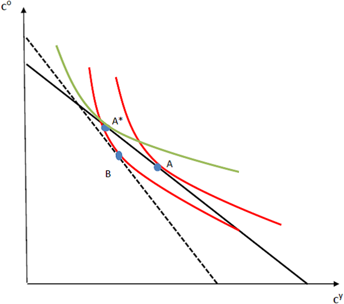
Figure 1. True vs. choice utility under pension schemes.
3.2 Decision rules
The budget constraints of an agent are


The private saving decision is determined by

and at the zero private-saving corner by

In line with the pension literature, s t ≥ 0 is imposed. Agents do not have any wage income as old; all they have is either interest income from prior savings or pension payouts. Allowing negative saving is tantamount to allowing borrowing against future pensions which we disallow; in any case, such borrowing is not possible/allowed in many countries.Footnote 13, Footnote 14
For later use, note

Hence, ∂s t/∂R t+1 > 0 holds when relative risk aversion is less than 1.
Assumption 3 (Risk-aversion)

a standard condition, well-known in the literature. Henceforth, we assume this is true.
In the absence of a pension scheme (τ = b = 0), the private saving decision satisfies u ′(w t − s t) = R t+1βu ′(R t+1s t). In this case, the non-negativity constraint on saving is never binding because of Inada conditions. If β = 0, then, of course, s t = 0 is possible; not otherwise. From the perspective of true utility, the optimal savings level $s_t^\ast$ satisfies

Myopia implies people place less weight on the future (β < β*), and therefore, care relatively more about current consumption—such agents save too little, i.e., $s_t < s_t^\ast.$ Indeed, ∂s t/∂β > 0 holds implying as β falls (the agent is more myopic), the less he saves, and the gap between his choice and true saving (s t vs. $s_t^\ast )$
 increases.Footnote 15 It is important to note that, in spite of ∂s t/∂β > 0, sufficiently high myopia (low-enough but still β > 0) will not drive agents to the zero-saving corner; since b = 0, and the agent earns nothing when old, Inada conditions will prevent that. For future use, note that when b > 0, sufficiently high myopia will drive agents to the own zero-saving corner.
4. A role for pensions?
4.1 PAYG
The government is aware that a change in pension benefits affects private saving via changes in the agent's after-tax endowment and his future income. Focus attention on a steady state. The government takes the agent's optimal saving response to its pension into account, s(b) and mandates a pension b by maximizing Ω*(b) = u(w − s(b) − b) + β*u(Rs(b) + b). The optimal level of b, if positive, is defined as the solution to

Using u′(c y) = βRu′(c o), dΩ*(b)/db reduces to

How does private saving respond to policy action? For the PAYG scheme, we find, in general,

leading to

The PAYG pension is designed to supplement an agent's own saving for retirement. Recognizing that, the agent cuts his own saving as forced saving via the pension increases. If the forced pension and his voluntary saving earned the same return, he would cut his own saving one-for-one in response to an increase in the pension. However, under dynamic efficiency, an extra unit devoted to the pension brings less future income than what private saving would have. As such, he does not reduce his own saving one-for-one; the crowding out—cf. equation (11)—is less than proportionate with the pension increase. Additionally, the present value of lifetime income under the pension, w + ((1 − R)/R)b falls as b rises (since R > 1), the agent's retired consumption falls, cf. equation (12).
Focus attention on equation (10). In the absence of myopia (β = β*), the second term on the r.h.s. of (10) drops out and hence the sign of dΩ*(b)/db is the same as the sign of 1 − R.
Proposition 1 [Aaron (Reference Aaron1966); Samuelson (Reference Samuelson1975)] Under Assumption 1 (dynamic efficiency), dΩ*(b)/db < 0 if there is no myopia (β = β*) implying there is no welfare justification for introducing or expanding a PAYG scheme.
Proof. See Appendix B. ■
In the absence of myopia, then, the optimal PAYG pension is b = 0. The agent dislikes the fact that his total retirement income, given by Rs(b) + b, falls with a rise in b.Footnote 16 This is clearly not what the government intended. Thankfully, the fall in Rs + b stops once s hits zero. This is so because of the crowding out of private savings (∂s t/∂b ≤ 0 for s t > 0); at a sufficiently high level of b, call it $\underline b$ , the corresponding level of private saving is zero, s t = 0. Thereafter, any further raising of b ($b \ge \underline b$
 ) has no effect on s as the non-negativity constraint on s binds—total retirement income is simply b which clearly rises with b!
The question is, how does the presence of myopia help reinstate a role for PAYG pensions? Notice when myopia is absent, the second term on the r.h.s. of (10) drops out implying ∂s(b)/∂b ceases to have any effect on the choice of b. Intuitively, the envelope theorem washes out the effect of b on s. Not so, when myopia is present. In that case, the choice self-views the effect of b on s differently from how the true self does—the true self discounts the effect on future saving at rate β* greater than the rate at which the choice self-discounts the same.
What about the first term on the r.h.s. of (10)? Since (11) tells us that ∂s t/∂b < 0 for s t > 0, it follows, that in the presence of myopia, the second term on the r.h.s. of (10) is negative. This means, for dΩ*(b)/db > 0 or PAYG pensions to have a shot at improving true welfare, the first term on the r.h.s. of (10), β* − Rβ, necessarily has to be positive. Equivalently, a necessary condition for a welfare rationale for PAYG pensions is sufficiently-strong myopia, β* > Rβ ⇔ β < β*/R—ordinary myopia, β < β*, is not enough!Footnote 17 Why? This is for the true self to benefit from the pension, the myopic agent's perceived effective return on private saving, Rβ, must be at least less than his true self's perceived return on the competing PAYG scheme, β*. (In the absence of myopia, this is not possible under dynamic efficiency.) Otherwise, even the true self would prefer no pensions.
Even when myopia is sufficiently strong, how big does b need to be? Recall $s_t < s_t^\ast$ —from the standpoint of true utility, a myopic agent is anyway saving too little. From (11), we know the agent cuts s t in response to the pension when s t > 0. A PAYG pension crowds out own saving which the true self dislikes, but as b rises beyond $\underline b$
 , consumption during retirement rises and that makes such a b attractive from the perspective of true utility. Knowing the true self likes $b > \underline b$
 , what level of b should the government choose? In the present setting with exogenous factor prices, there is no inherent dynamics in the economy. In which case, the pension level may be set, right away, at its long-run optimal value, the one that solves maxb u(w − b) + β*u(b) where

Note that b* does not replicate s* (defined in equation (8)). We have
Lemma 1 [Andersen and Bhattacharya (Reference Andersen and Bhattacharya2011)] A necessary condition for the PAYG pension b* to improve true welfare is β* > βR. For CES utility, a sufficient condition for true welfare to increase, i.e., Ω*(b*) > Ω*(0), is

Proof. See Appendix B. ■
For it to be optimal, the PAYG pension has to be large enough to drive voluntary private saving to the corner. Increasing the PAYG beyond that point makes it possible to increase old-age consumption, and thus, counteract the effect of the myopia. However, since the PAYG scheme is return-dominated, myopia (β*/β > 1) alone is not enough to deliver a welfare rationale for a PAYG pension. Sufficiently strong myopia relative to the rate of return (β*/β > R) is required for a welfare improvement to be possible.
Note from (14) that risk-aversion (or intertemporal substitution) plays a role: if ϕ = 1 or ϕ = 0, then Ω*(b*) = Ω*(0) and in either case, b* does not improve welfare. In Appendix B, we present a numerical example of a configuration of parameters satisfying β* > βR that also satisfies (14) for all ϕ ∈ (0, 1).
4.1.1 Fully funded pensions
Consider, next, a mandated FF pension scheme with contribution rate d (τ t = d and b t+1 = Rd). The FF-pension also crowds out voluntary saving, and since the returns are the same, the crowding out is one-to-one, i.e., analogous to equation (11), we have

Hence, a mandated FF pension contribution only affects total saving if it is sufficiently large, $d \ge \underline d$ . The critical contribution level $\underline d$
 is defined by ${u}^{\prime}( w-\underline d ) \equiv R\beta {u}^{\prime}( R\underline d )$
 . The contribution rate maximizing long-run true welfare is determined by (assuming voluntary saving is driven to zero, $d \ge \underline d$
 ) maxd u(w − d) + β*u(Rd) and the optimal level d* is determined by the first-order condition

Notice d* = s*. This means a FF program with contribution equal to s* can exactly replicate the desired retirement saving of the true self. Of course, private saving is zero but retirement saving under the FF scheme is exactly what true utility demands. It follows directly that
Lemma 2 A FF pension with contribution rate d*—determined by (15)—generates higher true steady-state utility when compared either to what is possible under laissez faire (τ = b = 0) or an optimal PAYG pension (b*).
Note, the relationship between the optimal PAYG pension, b*, and the FF pension, d*, is, in general, ambiguous $(b^*\displaystyle{ > \over < }d^*)$ .Footnote 18
4.2 Transition from a PAYG to a FF pension system
A PAYG pension has the advantage that it provides, up-front, the current old with a pension, and therefore offers an immediate remedy to their low old-age consumption problem. To that end, suppose the government introduces the long-run optimal PAYG pension at level b*, cf. (13). From Lemma 2, we know that continuing this program is not in the interest of long-run welfare: an optimal FF scheme would do better. The question is: is it possible to make the transition to a FF scheme under the Pareto criterion, the constraint that utility for each cohort remain at least as high had the PAYG pension scheme b* persisted?
To operationalize this question, assume that the long-run optimal PAYG scheme (b*) installed at t and kept in place up to date t + m (m > 0). Recall, this is consistent with every cohort up to t + m being at the zero private-saving corner. Also recall for b* to be welfare-improving, agents must display sufficiently strong myopia, i.e., β*/β > R. At t + m, the government ushers in a FF scheme by mandating the then young to contribute d t+m > 0 to the scheme. (It is possible that private saving re-emerges, we denote it s(b*, d t+m)); recall, though, any increase in d is crowded out one-for-one by a decline in s.) Denote the PAYG pension to be received by these retirees by b t+m+1, i.e., we allow for the possibility that the level of the PAYG scheme is changed after the FF scheme is introduced. True life-time utility for the cohort born at t + m under this policy package is

which may be rewritten as

Note that the term (R − 1)d t+m captures the return gain to switching from the PAYG to the FF scheme. To foreshadow, this extra income/welfare will be crucial for a successful transition under the Pareto criterion.
The first issue is whether the cohort born at t + m sees a welfare gain from the mandate of a FF pension contribution, d t+m, on top of their PAYG pension contribution b*?
Lemma 3 True life-time utility of cohort t + m, $\Omega _{t + m}^\ast$ , can be improved by mandating them to contribute at the margin to a FF scheme in addition to their PAYG contribution of b*:

Proof. See Appendix C. ■
Note that with the PAYG pension at b*, private saving is already at zero; hence adding on an incremental FF pension does not distort saving: ∂s(b*, d t+m)/∂d t+m = 0. The marginal unit earns R via the FF scheme which is better than what it would have earned under the PAYG scheme. Hence, on the margin, continuing the initial PAYG scheme and adding a (small) mandated FF pension makes the inaugural set of agents better off.
The welfare gain may be used to phase out the PAYG scheme under the Pareto criterion. Define

as the lifetime utility to cohort t + m had the PAYG pension b* continued unchanged. It follows, that for cohort t + m, the Pareto condition is $\Omega _{t + m}^\ast \ge \Omega _{t + m}^{{\ast} {\rm PAYG}}$ where
where

where $\Omega _{t + m}^\ast$ captures the changes ushered in by adding a mandated FF contribution, d t+m, over and above the PAYG contribution of b* as well as the possibility that this cohort will see a PAYG benefit of b t+m+1 instead of b*. Lemma 3 implies $\exists d_{t + m} > 0$
 such that $\Omega _{t + m}^\ast \ge \Omega _{t + m}^{{\ast} {\rm PAYG}}$
 holds. Then, there exists a b t+m+1 < b* such that

Hence, the gains from phasing in the FF pension (d t+m > 0) may be used, under the Pareto criterion, to bring down the level of the return-dominated PAYG pension (b t+m+1 < b*).
The upshot is that PAYG and mandated FF schemes are both appropriate government interventions for myopic agents. The FF scheme is just better in the long run: a unit of funds taken from the PAYG contribution and shifted to the FF scheme produces a return gain. Yes, in a literal sense, it is true that a transition from a PAYG to a FF scheme requires some cohorts to “pay twice” but, unlike in the classical results (see Proposition 1) derived with time-consistent agents, such cohorts are not worse off.
What happens to generations further down the transition, indexed t + m + j with j > 0? What does the trajectory of d and b look like under the Pareto criterion? Consider, for the sake of argument, a very simple, stylized scheme that sets d t+m = κb*, κ ∈ (0, 1) so that

i.e., right from the start of the transition, the overall contribution rate (summed across both pensions) is raised relative to the PAYG world. (Many other such schemes can be constructed—see below.) This implies, for example, d t+m+1 = (1 + κ)b* − b t+m+1, that is, if we generate a declining sequence for b t+m+1, we automatically generate an increasing sequence for d t+m+1—if the PAYG is phased out, the FF is phased in. The equal utility condition for period t + m, $\Omega _{t + m}^\ast{ = } \Omega _{t + m}^{{\ast} {\rm PAYG}}$ now reads

apropos Lemma 3, there exists a κ > 0 ensuring b t+m+1 < b*, the start if the declining sequence for b. Below, we show it is possible to engineer a transition which leaves every cohort along the transition at least as well off as in the counterfactual persistent PAYG scheme. This is our flagship result.
Proposition 2 For an economy with an existing PAYG pension b*, there exists a policy package $\big \{ {b_{t + m + j}, \;d_{t + m + j}} \big \} _{j = 0} ^\infty$ implemented at t + m which satisfies the Pareto condition

with b t+m+j following a decreasing sequence and reaching 0 in finite time, and d t+m+j following an increasing sequence converging to d*, allowing d* to be implemented.
Proof. See Appendix D. ■
Along the transition path, the PAYG-pension is gradually phased out, and the FF pension expanded, ensuring cohorts have the same life-time true utility had the PAYG-world persisted. Eventually, the PAYG pension is fully phased out (b t+m+j = 0), and replaced by a FF pension (d t+m+j > 0 for all j ≥ 0). Once that happens, all cohorts are necessarily better off than under the PAYG scheme. Notably, it is possible to implement d* which delivers the optimal level of saving, s*, from the point of view of the true self.
Of course, there may be multiple Pareto-improving transition paths. Proposition 2 outlines a particular path where utility for cohorts is kept at the PAYG level until the pension is fully phased out, after which, subsequent future cohorts get to enjoy higher utility. Other paths, where some of the future gains are distributed up-front such that all cohorts are strictly better off, are possible.
5. Endogenous factor prices
Everything up to now has been derived for the case of exogenous factor prices. The case with endogenous factor prices is more challenging since changes in the pension system trigger general equilibrium responses to wages and interest rates, which in turn, impact saving decisions. Recall, our approach differs from usual Kaldor–Hicks one because we implement the actual policy and explicitly impose that utilities be no less than in the pre-reform case along the actual, not hypothetical, transition path. This is a non-trivial task when factor prices are endogenous. However, before we get there, we settle up some issues regarding dynamic competitive equilibria for this economy.
5.1 Equilibrium
Henceforth, we assume factor markets are perfectly competitive, and thus, factors of production are paid their marginal product in each period, i.e.,

and

where f′(k t) > 0 and f′′(k t) < 0 and, hence R′(k t) = f′′(k t) < 0 and ω′(k t) = −k tf′′(k t) = −k tR′(k t) > 0.
In several places below, we will assume
Assumption 4

which holds for a standard production function such as the Cobb–Douglas, $f( k ) = k^\alpha , \;$ α ∈ (0, 1) where η(k) = α − 1. It also holds for a CES production function f(k) = [αk (1−σ)/σ + (1 − α)]σ/(σ−1) with α ∈ (0, 1) and σ ≥ 1.
In passing, note that

This means if k rises, capital income (R(k)*k) also rises if Assumption 4 holds. This fact will be useful in Propositions 5 and 6.
Throughout, a dynamically-efficient economy is assumed.
Assumption 5

The economy without any government intervention—laissez faire—is identical to that studied in Diamond (Reference Diamond1965). We have from (4), and using (18) and (19),

which implicitly defines the equilibrium law of motion for k : k t+1 = ψ(k t, β, 0). In the case of a time-invariant PAYG scheme (τ t = b t+1 = b > 0), the equilibrium condition in the capital market is k t+1 = s t, and hence, we have

which implicitly defines the equilibrium law of motion for k:

All competitive equilibria with PAYG pensions are characterized by the sequence $\{ {k_{t + 1}} \} _{t = 1}^\infty$ defined by (21) and the government budget constraint. For a FF scheme with contribution rate d (τ t = d and b t+1 = Rd), the equilibrium condition in the capital market is k t+1 = s t + d t, and hence, the corresponding equilibrium law of motion for k is

Define
(1) k: the steady state capital–labor ratio in the absence of any government intervention, defined as laissez faire, the solution to k = ψ(k, β, 0).
(2) k b: the steady state capital–labor ratio for a given PAYG pension b which solves k b = ψ(k b, β, b).
(3) k*: the steady state capital–labor ratio in the absence of both myopia and pension which solves k* = ψ(k*, β*, 0).
We make all standard assumptions ensuring the existence of a unique and stable—see Appendix E—steady-state equilibrium, see e.g., De la Croix and Michel (Reference De La Croix and Michel2002):
Assumption 6 (Stability)

In particular, assume 0 < ψ k(k b, β, b) < 1 (this assumption is necessary for k b—see below—to be locally stable).
5.2 PAYG pensions
As before, we start by establishing the impact on private saving (or capital) of myopia and pensions. It is easy to verify (see Appendix E) that

implying the bigger the weight (β) agents assign to the future, the larger the saving due to consumption smoothing, and therefore larger the capital–labor ratio at any point in time. Similarly, in Appendix E, we show

meaning that the PAYG pension crowds out saving and leads to a lower capital–labor ratio. Assume a PAYG scheme is introduced (unanticipated) in period t such that each young pays b > 0 (not too large) to each old in that and all future periods. From equation (23), it follows that upon introduction of the PAYG pension, the capital stock is declining along the equilibrium trajectory and eventually reaches k b, defined in section 5.1. Since these results hold in steady state, the next result is immediate.
Lemma 4

Proof. Since ∂k/∂β > 0 (see Appendix E) and β < β*, k is smaller than the capital stock in a corresponding economy with non-myopic households. Myopia implies agents save too little, and hence, the capital stock is lower. Since ∂k/∂b < 0 (see Appendix E), k b is smaller than the capital stock in the absence of a PAYG pensions system, k b < k. ■
From Lemma 4, recall k <k* holds, meaning the underlying “undersaving” issue faced by myopic agents persists in the case with endogenous factor prices: myopic agents hold too little capital. Under dynamic efficiency (R(k) > 1), if policy action can incentivize these agents to hold more capital, then steady-state welfare would rise. The problem, as before, is that a higher pension reduces the capital stock. There is, however, one big difference as compared to the case with exogenous factor prices. With endogenous factor prices, as the pension crowds out physical capital, the return to capital would rise (an effect absent earlier), raising the incentive to hold more of it. The equilibrium, therefore, has both voluntary savings and the PAYG pension.
Proposition 3 Suppose Assumptions 1–6 hold. (a) For introduction of a PAYG pension scheme to increase true steady-state welfare over laissez faire, it is necessary that

holds, (b) it is possible that, upon introduction, true welfare improves both for the inaugural generation and for each and every subsequent cohort, and (c) k* (corresponding to β*) cannot be replicated by a PAYG pension.
Proof. See Appendix F. ■
It is easy to construct numerical examples where (a) voluntary saving (in the form of capital) and public pensions co-exist, and (b) the optimal pension is positive even under dynamic efficiency.
5.3 FF pensions
Under a FF scheme, the decision problem for an individual born in period t is

Since s and d have the same return, they are perfect substitutes and only total saving k = s + d matters. It follows that voluntary savings s decreases one-for-one with an increase in d for s > 0. For d so high that s is driven to the zero corner, we have u ′(ω(k t) − d) > βR(k t+1)u ′(R(k t+1)d).
Proposition 4 Setting mandatory pension savings at the level d = k* > k implements what the long-run true self wants. Steady-state welfare under such a program is, therefore, higher than in laissez faire and for any PAYG pension.
The undersaving problem can thus be addressed by a proper choice of the mandated pension contribution. This, however, is a steady-state result, and therefore not of much use in solving the immediate problem for households with inadequate savings.
It is important to note that, in the FF world, even though the entire capital stock is being held by the pension funds, the ownership of these funds lies with the agents (via individual accounts) and not the government.
5.4 Transition to a fully-funded system
Is it possible with endogenous factor prices to make a transition from a PAYG to a FF system under the Pareto criterion so that no cohorts are made worse off along the transition path?
5.4.1 Gain from introducing a FF pension
Let the PAYG pension scheme b be introduced in period t. Is there at some point in time—during adjustment to steady state or in the new steady state—a welfare gain from introducing a FF pension? To answer this question, consider introduction of a mandatory contribution larger than the initial capital stock, d t+m > k t+m in period t + m, implying full crowding out of private savings (s t+m = 0 and k t+m+1 = d t+m), where the capital is predetermined at its value at t + m. We have
Proposition 5 At any point in time t + m, m > 0 after the introduction of the PAYG pension scheme, true life-time utility $\Omega _{t + m}^\ast$ can be improved by introducing a FF pension contribution d t+m > k t+m, under assumption 4 and

Proof. See Appendix G. ■
The assumption on η(k t+m)—see Assumption 4—ensures that the return to capital is not “too sensitive” to the capital stock. Sufficiently-strong myopia (β* > β/(1 + η)) is necessary and sufficient for phasing in of a FF pensions system (d t+m > 0) to have positive welfare effects on all subsequent cohorts.Footnote 19 Assuming this holds, it is possible to reduce the PAYG pension while satisfying the Pareto condition, i.e., there exists a b t+m+1 < b and d t+m > k t+m such that

This is the first step in a transition out of the PAYG scheme.
5.4.2 Complete phasing out of PAYG pensions
To work out an explicit case with full phasing out of a PAYG pension under the Pareto criterion, we first analyze an economy that has reached a steady-state with a PAYG pension b > 0 and the associated capital stock, k b, and associated life-time utility, Ω*PAYG.Footnote 20 At t + m > t, an unanticipated announcement is made that a phasing out of the PAYG scheme and a transition to a FF system is underway with a goal of achieving the optimal long-run level of capital d = k*.
We are looking for a policy sequence $\{ {b_{t + m + j}, \;d_{t + m + j}} \} _{j = 0}^\infty$ which satisfies the Pareto condition

where k t+m = k b and k t+m+j+1 = d t+m+j, implies

and the introduction of increasing contribution to or phasing in of the FF pensions system:

i.e., the pension to the current old (in period t + m) is the pension from the PAYG regime and the current young finance this, where the contribution is at the PAYG steady state level. The current young are also required to contribute to the FF scheme with a contribution d t+m.
Proposition 5 gives conditions ensuring that cohort t + m are better off when a FF pension is introduced on top of the PAYG pension. Under the Pareto criterion, this welfare gain may be used to bring down the PAYG pension this cohort receives (without hurting them). The next cohort sees an increase in their wage income due to a higher capital stock. That, as well as the reduced contribution to the PAYG pension, enables further increases in FF pension contribution resulting in additional increases in the capital stock and enabling a greater reduction in the PAYG pension they receive. Hence, the first step has more savings and a reduction in the PAYG pension. Downstream the change in savings and thus the capital stock also affects wage. Cohort t + m + 1 will have a higher wage rate because the capital stock has increased (compared to status quo), and this make them better-off. Under the Pareto condition this creates room to decrease the PAYG pension further. Working out this dynamics in detail generates the following result.
Proposition 6 Assume the transition starts from a steady-state equilibrium with a PAYG pension b and associated capital, k b. Under the assumptions—see Assumption 4—that η(k b) > −1 and β* > β/(1 + η(k b)) there exists a trajectory satisfying the Pareto criterion, where the PAYG pension is entirely phased out, and the FF pension expanded so that k* is reached in the long run.
Proof. See Appendix H. ■
The above shows the existence of a transition path assuming that the economy is initially in steady state equilibrium with a PAYG pension b. The result can be considerably generalized.
Proposition 7 Assume that the transition starts from an arbitrary date t with a PAYG pension b t. Assume

where

Then there exists a trajectory satisfying the Pareto criterion, where the PAYG pension is phased out, and the FF pension is expanded.
Proof. See Appendix I. ■
The bottom line is this. Starting from an initial setting with a PAYG pension in place, it is possible to replace it with another mandated scheme, the FF scheme, which not only preserves (even increases) the benefits of the PAYG in terms of its forced-saving character but also generates a higher return. And along the transition, no one is hurt. Note that once the PAYG scheme is fully phased out, cohorts further downstream are made strictly better off.
5.5 Intuition
We now summarize our intuition about the entire transition. There are many parts, many moving parts, so we approach each one in turn. Suppose a standard Diamond economy is at a laissez faire (LF) steady state with k = k LF. Since this was reached under choice preferences and agents are myopic, it is clear that k LF < k* where k* is the level of k attainable under true preferences. At any date under LF, all retirees have too low retirement consumption (relative to what they would have had under true preferences) because they saved too little due to their myopia (Figure 2).

Figure 2. Transitions.
Now, suppose the government starts an optimal PAYG scheme, b t, one derived by maximizing true utility. The scheme, by its very nature, transfers resources from the young to the retired. The young respond by cutting their own saving even further but they end up with more retirement consumption. Their choice utility does not like this but under true preferences, they are made better off. Because saving is increasing in its return, and the PAYG scheme is return-dominated, the latter does not lead to complete crowding out of private saving. Also, the initial old at the point the policy was initiated are made better off because the pension they receive from the initial young is higher than their LF retirement saving. Downstream, all future generations have higher true utility than under the LF.
At some point, the PAYG transition is completed and a new steady state, k PAYG is reached. By that time, b t has converged to its steady state level, b*. To reiterate, this point has higher true utility than at k LF, lower personal savings but higher retirement consumption. The retirees are receiving b*. Now, the government initiates a FF scheme, asking the young at that date to not only contribute b* for the current retired but also mandate them to contribute d 1 into the FF program. Since d and k earn the same return, they are perfect substitutes: a rise in d leads to a one-for-one decrease in k, so that, in fact, k 1 = d 1 > k PAYG. In other words, d 1 ensures complete crowding out of personal savings. (Recall, by assumption, they cannot borrow.) In effect, their myopia is rendered impotent. This, recall, is not achieved under the PAYG scheme. It is in this sense that the FF scheme is better at “managing” myopia than the PAYG scheme.
This mandate also does several things. It raises downstream w but lowers downstream R (but even with the reduced R, agents benefit from getting a return R on their contributions vs. 1 in the PAYG scheme). Overall, under the conditions laid out in Proposition 6 (the ones relating to sufficiently strong myopia and low η) there is a welfare gain, and under the Pareto criterion, this can be “taxed away” and a PAYG b < b* can be offered to these young. The transition proceeds with d rising and b falling until a point where b = 0; the PAYG scheme is fully phased out and all that remains are mandated pension contributions, d*. As we have shown in Proposition 6, d* can even replicate k*.
5.6 Numerics
Below, we undertake a short computational analysis to showcase some of the crucial features of the transitional dynamics. The idea is not to conduct a serious calibration exercise but rather to offer some broad brushstrokes and quantitative insights within the confines of our two-period model. The exercise serves two purposes. It allows us to include population growth, and also helps us demonstrate the empirical relevance of the transition we have derived.
Consider a baseline economy where $f( k ) = Ak^\alpha$ and $\Omega _t^\ast{\equiv} ( c_t^y ) ^{1-\phi }/( 1-\phi ) + \beta ^\ast ( ( c_{t + 1}^o ) ^{1-\phi }/( 1-\phi ) )$
 and $\Omega _t\equiv ( c_t^y ) ^{1-\phi }/( 1-\phi ) + \beta ( ( c_{t + 1}^o ) ^{1-\phi }/( 1-\phi ) )$
 . There are five primary parameters to choose, ϕ, β, β*, α, and A. We set them as follows: ϕ = 0.8, β = 0.2, β* = 0.9, α = 0.22, and A = 5. A and α are chosen to deliver a 30-year interest rate of near 2.5 (or an annual real interest rate of around 3%). A discount factor of β = 0.2 implies an annual, one-period discount rate of 6%. We chose a relatively high β* to show that we could implement policies that take the economy close to the Golden rule. The average ratio of public pensions plus old-age cash benefits to GDP across OECD countries in the past three decades has been about 5%. We chose ϕ to come close to that number. In one setting, we allow for population growth 1 + n where n is set to 0.2 (annualized rate of 0.6% close to OECD averages in the past three decades). Below, we present some additional examples.
We report results from three sets of experiments. In the first, the economy is at a steady state with retirees receiving, b*, the optimal PAYG pension. The transition starts with the inaugural young generation being asked to pay b* to the current retirees and contribute d t to the FF scheme. As explained in the text, we go on to compute the sequence of b t+j and d t+j ensuring lifetime utility during the transition is held equal to the lifetime utility at the pre-policy steady state. Once the b t+j sequence has been fully phased out, we allow the resulting welfare gains to accrue to future generations. The second experiment is the same as just described, except for the transition starts at some date before the steady state under the PAYG scheme has been reached. And the last experiment is like the first except we allow for population growth.
5.6.1 Transitions
In the first experiment, the mandated contribution is introduced and gradually stepped up, see Figure 3a. At first, the PAYG pension can only be reduced marginally under the Pareto condition. Downstream when the gains from having contributed to the FF scheme become larger, the PAYG pension can be reduced more sharply, and eventually fully phased out, and the optimal steady state FF contribution fully phased in.

Figure 3a. Pareto-improving transition starting from and away from a PAYG steady state.

Figure 3b. Transition from a PAYG system to a FF system with population growth.

Figure 3c. Range of myopia satisfying the Pareto condition (24).
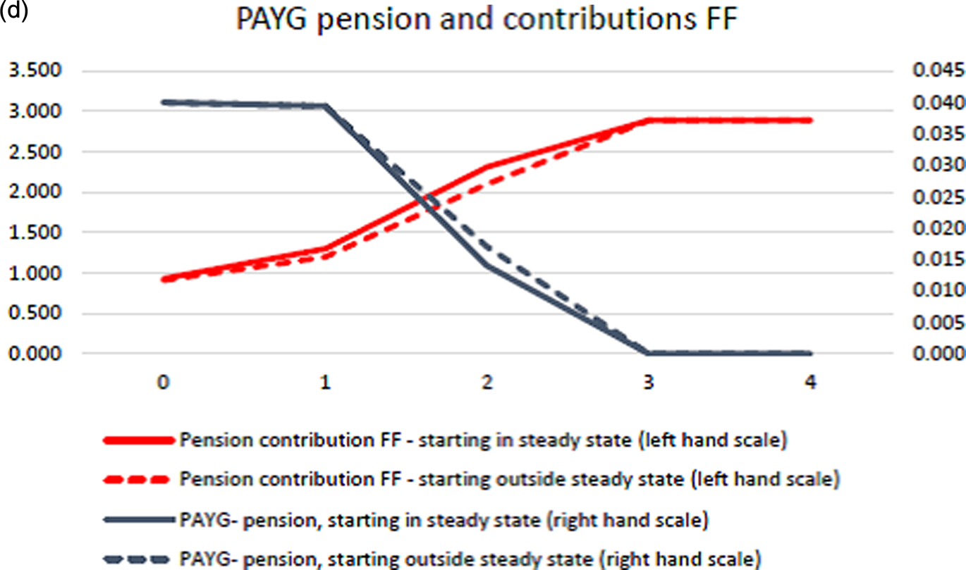
Figure 3d. Fast transition.

Figure 3e. Slower transition.

Figure 4. Contribution rates, occupational labor market pensions, and total pension expenditures for public sector and contribution-based pension funds. Note: Contribution rates applies to DI/CO collective agreements. Since 2009 contribution rates have been identical for blue- and white-collar workers. Expenditures: data 2015 onward are projected expenditures. Data source: Ministry of Finance (2017).

Figure 5. (a) LHS and RHS and (b) ϕ*.
From the point where the PAYG pension has been fully phased out, cohorts are strictly better off than in the PAYG steady state, the start of the transition. Implementing the FF pension outside steady state (before the capital stock has converged to the steady state value associated with the PAYG pension b*) is possible but has a longer transition period. FF contributions have to be phased in more gradually, and PAYG pensions phased out more slowly to satisfy the Pareto condition. This is partly because the policy is introduced with retirees receiving the long run PAYG pension b* even though the dynamics under the PAYG pension has not worked itself out fully. Finally, it is seen that population growth makes the transition more slow, see Figure 3b, but still possible. Note that the steady state is different from the case reported in Figure 3a due to the population growth. With population growth, the return difference between the PAYG scheme and the FF scheme is smaller, and this explains why the transition period is longer. Note, in each case, the transition to the FF scheme is completed within four to five generations.
5.6.2 Strength of myopia
Proposition 5 shows that a necessary and sufficient condition (for the phasing out of a PAYG pension system and the phasing in of a FF one) to satisfy the Pareto criterion is the condition (24). For Cobb–Douglas technology, (24) reduces to a simple restriction on parameters:

which may also be viewed as a condition on the strength of myopia needed.
Wang et al. (Reference Wang, Rieger and Hens2016) report estimates of annual discount factors and present bias for 53 countries (see Figure 3 in their paper), where present bias is measured by the value of γ ∈ (0, 1) in the life-time utility: $u( {x_0, \;x_1, \;\ldots , \;x_T} ) = u( {x_0} ) + \gamma \mathop \sum \nolimits^T_{t = 1} \delta ^t u( {x_t} )$ and δ ∈ (0, 1) is a discount factor. Our corresponding measure of myopia (25) isFootnote 21

Wang et al. (Reference Wang, Rieger and Hens2016) report values of γ ranging from approximately 0.01 to 0.99 and δ ranging from approximately 0.78 to 0.9. This implies β*/β ∈ (1, 13.1) in the data. Figure 3c plots 1/α from which it is clear what the minimum β*/β has to be for (25) to be satisfied. For instance, when α ≈ 0.4, (24) is satisfied for β*/β ≈ 2.5 which lies in the range reported in Wang et al. (Reference Wang, Rieger and Hens2016).
5.6.3 Additional examples
We close by offering two additional examples that offer some reassurance of the robustness of our findings. In the first example, ϕ = 0.99, β = 0.15, β* = 0.73, α = 0.21, and A = 9. In this case, β*/β ≈ 4.86 > 1/α. For this example, the optimal b in the steady state is 0.04; the transition to FF is completed in three generations.
The next example uses ϕ = 0.8, β = 0.15, β* = 0.8, α = 0.2, and A = 5. In this case, β*/β ≈ 5.3 > 1/α and the optimal b in the steady state is 0.13; the transition to FF takes longer to complete, five generations.
6. Conclusion
In the pension literature it is well-established that a PAYG pension has the advantage of delivering pensions up front to current pensioners. The downside is that this scheme is return-dominated by a funded scheme, which thus delivers higher long-run welfare. However, the phasing in of such a scheme runs over several decades. This disadvantage of the PAYG scheme has prompted the question whether it can be phased out without hurting any cohorts along the transition. The literature has largely answered this question in the negative.
This paper argues that the discussion on pension system transition has overlooked the reasons why pension schemes were introduced in the first place. A key argument is that agents do not save enough due to their present bias. Starting from this observation, we show that it may be optimal to introduce a PAYG scheme in the first place, not only because it is beneficial to the inaugural old, but also because it addresses an undersaving problem. However, this scheme is return dominated by a funded scheme. A switch to the latter scheme is a good idea but it would endanger the incomes of the current generation of retirees. We show that a transition is possible and yet no cohorts are worse off. In a way, our results speak to a “division of labor” between PAYG and FF pensions: the former takes care of the needs of the current retirees and the latter, because of the present bias, proves beneficial to both current and future generations. This last statement has important implications for pension policy design.
As outlined in the Introduction, our analysis informs the debate on pension policy design. The classic conundrum facing policymakers has been the following. There is a generation of current retirees that need a pension. At the same time, the current working generation needs to be transferred to a FF scheme. How to get the young to contribute to paying a pension to the initial generation of retirees and get them to contribute to their own FF scheme? Conventional thinking stops here because the burden on the transition generation from having to pay twice is believed to be too much for any generation to have to endure. This has been the major sticking point in the discussion about pension reform. Our analysis argues the transition may not be as burdensome as believed.
In the current paper, we have focused on the basic differences between PAYG and funded pension schemes to address the fundamental transition issue with a singular focus on intergenerational distribution. Intragenerational heterogeneity has been analyzed in the literature and distributional or risk-sharing motives have been used to generate an argument for PAYG pensions even under dynamic efficiency. Intragenerational heterogeneity would raise legitimate informational concerns although, at least in theory, there can be a flat rate pension with minor informational demands. More sophisticated schemes would have either contributions or benefits differentiated across types. This is an interesting area of research in the future. Our focus, of course, is on inadequacies in saving-for-retirement alone and the use of mandated schemes to that end.
As we have shown, once the mandate is high enough, the voluntary retirement saving disappears and further increases in the contribution mandate raises agents' welfare. Problems would emerge if the government mandate was so aggressive as to warrant borrowing by the young, but as Andersen and Bhattacharya (Reference Andersen and Bhattacharya2019) have shown, there is no welfare case to choose such a high mandate. An implication of this idea is the following. Suppose there were some agents who did not suffer from time inconsistency. The welfare of such agents under laissez faire and under the government mandate would be identical.
Finally, we take up a philosophical point. In our study, and in many others, the assumption is that the government is paternalistic and evaluates welfare differently than the citizens. In a sense, then, the Pareto-improving transition we derive is possible from the government's point of view (true preferences of the agents, not their choice preferences).Footnote 22 One may ask, why do we evaluate welfare from the point of view of “true” utility? And if people are to vote on such schemes, would voters use their choice or true preferences to decide? These are deep, philosophical questions which deserve independent inquiry. In our defense, all we can say is the following. First, ours is a normative analysis showing that such a transition is possible; it is not a political-economy analysis. Second, the distinction between true and choice preferences is, in one form or the other, standard in the normative behavioral economics literature. Third, mandated pensions can be seen as an institution—a commitment device. Forward-looking agents who recognize their own self-control problems and see the commitment power of this institution may well support this because it appeals to the “better angels of their nature.”
Acknowledgements
We thank three anonymous referees and the editor, David de la Croix, for their encouragement and constructive input. We also acknowledge financial support from the Danish Council for Independent Research (Social Sciences) under the Danish Ministry of Science, Technology and Innovation.
Appendix A: The Danish experience
Funded pension schemes play a significant role in e.g., the Netherlands, Canada, and Denmark. In the following, we outline the developments in Denmark as an example of a transition from a system relying mainly on PAYG pensions to a system where funded pension schemes have taken on a substantial role.
While achieving a welfare state objective of ensuring some minimum income level for all pensioners, there was a growing concern over the adequacy of the pensions, especially due to the implied low replacement rates for medium- and high-income groups. Various steps were taken to address this problem, but the pivotal change appeared in the late 1980s. The social partners—employers and employees—took initiative to broaden and extend occupational funded pension schemes. Previously supplementary pension scheme existed for particular groups e.g., highly educated, and the decisive move was to extend this to most of the labor market. Figure 4 illustrates how contribution rates to funded occupational pension schemes have developed since the early 1990s for large groups of blue- and white-collar workers in the private labor market. Although these occupational pensions were voluntary in the sense of being the outcome of negotiations between the social partners, participation is mandatory for the individual worker. There is evidence that household net savings has increased as a result of these schemes. In an influential study, Chetty et al. (Reference Chetty, Friedman, Leth-Petersen, Nielsen and Olsen2014) use Danish data and exploit increases in mandated pension contributions at job shifts to identify strong positive effects of mandated contributions on household savings.
The increase in coverage and contribution rates has naturally implied an accumulation of substantial funds now amounting to more than 200% of GDP, the highest level among OECD countries. It takes several decades for occupational funded pension scheme to mature in the sense that contributions have been made over an entire work career and pension benefits are enjoyed based on such contribution for the entire pension period. The system is thus still maturing.
Figure 4 shows pension payments from contribution-based pension funds as a share of GDP, and the increasing trend until about 2,045 reflects the maturation of the scheme. Interestingly, public expenditures are falling as a result of individuals having larger private pensions via means-testing receive less in public pensions, as well as increases retirement ages. Pensions from funded scheme would form 2,045 dominate tax-financed pensions. Despite an increasing old-age dependency ratio on par with the OECD average, public pension expenditures are falling and increasingly targeted low-income groups. It is noteworthy that criteria for fiscal sustainability are satisfied and that the system delivers the highest replacement rates among EU countries, see European Commission (2018, 2019).
Appendix B: Proof of Lemma 1
The contribution rate under a PAYG pension scheme is τ t = b t, and true life-time utility therefore reads

Notice that with exogenous factor prices we immediately reach steady state if implementing a time-invariant pension (b t+j = b for all j ≥ 0). Denote this level of PAYG benefits for b, which we consider in the following (and, hence, suppress time subscripts). Agents are better-off under the PAYG scheme compared to laissez-faire if

Private savings given the level of pension, s(b), is u ′(w − b − s(b)) = Rβu ′(Rs(b) + b) if s > 0 and u ′(w − b) > Rβu ′(b) if s = 0. For s > 0 we have

We have, using (1)–(3), the results above and assuming time-invariant PAYG pensions system, that (remember, R > 1 is assumed)

Hence, if the PAYG pension b should be welfare improving it is necessary that it be high enough that private voluntary pensions savings is fully crowded out. Define b: s(b) = 0. If private savings is zero (implying u ′(w − b) > Rβu ′(b)), the optimal b is a solution to $\mathop {\max }\limits_b u( {w-b} ) + \beta ^\ast u( b )$ and the associated first-order condition is u ′(w − b) = β*u ′(b). Hence, for b* > b being socially optimal when s = 0 it is necessary that β*u ′(b) > Rβu ′(b) which requires β* > Rβ, i.e., with sufficiently strong myopia there is a welfare case for a PAYG pension. Note, this is a necessary condition; for true utility to increase, it is required that Ω*(b*) > Ω*(0), see Andersen and Bhattacharya (Reference Andersen and Bhattacharya2011) for details.
Assuming a CES utility function u(c) = (c 1−ϕ/(1 − ϕ)), ϕ ∈ (0, 1), we have that savings in equilibrium s and optimal PAYG pension b* are given by a solution to (w − s)−ϕ = Rβ(Rs)−ϕ and (w − b*)−ϕ = β*b*−ϕ, respectively. These give

Substituting these into the true utility function Ω* = ((c y)1−ϕ/(1 − ϕ)) + β*((c o)1−ϕ/(1 − ϕ)) and performing some calculations gives that for Ω*(b*) > Ω*(s) it is necessary and sufficient that (remember, ϕ < 1 is assumed)

One period in the model is approximately 30 calendar years. Assuming an annual subjective rate of time preference of about 10% gives the one period discount factor β ≈ 0.06. Furthermore, assuming that β* = 1 and R = 2.42, which implies annual real interest rates of 3%, satisfying the necessary condition β* > Rβ, gives the following parameter values: β = 0.06; R = 2.43; β* = 1. These give the results shown in Figure 5.
As can be seen from Figure 5a, the LHS > RHS holds for all ϕ ∈ (0, 1) implying that a PAYG pensions system is welfare improving. This result holds for β = 0.06 and it is interesting to see how the result depends on the value of β.
The black line in Figure 5b shows the maximum value of ϕ, i.e., ϕ*, for which LHS > RHS for different β. The line starts at β ≈ 0.14 implying that LHS > RHS for all ϕ ∈ (0, 1) and 0 < β ≤ 0.14. For β > 0.14, ϕ* is decreasing in β implying that the parameter space in ϕ for which LHS > RHS is decreasing in β. The necessary condition β* > Rβ is fulfilled for all βs where LHS > RHS (which is logical since it is a necessary condition).
Appendix C: Proof of Lemma 3
True life-time utility is affected by mandated contributions to a FF pension scheme as follows:

With PAYG contribution b t+m+1 = b*, we have s = 0 implying ∂s( ⋅ )/∂d t+m = 0. Hence, evaluating the welfare effect for d t+m = 0, b t+m+1 = b* and using that u ′(w − b*) = β*u ′(b*) gives

Hence, on the margin, continuing the initial PAYG scheme and adding a (small) mandated FF pension makes agents better off.
Appendix D: Proof of Proposition 2
Let

i.e., from the start of transition the contribution rate is raised relative to the PAYG world, κ > 0. This implies d t+m+1 = (1 + κ)b* − b t+m+1 i.e., if we have a declining sequence for b t+m+1 we get an increasing sequence for d t+m+1; if PAYG is phased out, the FF scheme is phased in. Using this in the equal utility condition in (16) for period t + m gives

and given Lemma 3 there exists a κ > 0 ensuring b t+m+1 < b*. For period t + m + 1 the equal utility condition can now be written as

or

Since

it is implied

and since b* − b t+m+1 > 0 this requires b t+m+2 < b t+m+1. Similar reasoning holds for subsequent periods. If d* has not been reached along this transition path, then clearly it is possible to increase d to reach this level, since no compensation is needed any longer when the PAYG pension has been eliminated.
Appendix E: Proof of Lemma 4
It is easy to verify that the partial derivatives of (21) are

It is assumed that the denominator in these expressions is strictly negative, which is under Assumption 6.
The steady state capital stock k for a given PAYG pension b is given by the k solving

Hence,

where it is assumed that 0 < ψ k(k, β, b) < 1, which holds under Assumption 6.
Appendix F: Proof of Proposition 3
F.1 Part A
F.1.1 Steady state
True steady state welfare is

The effect of an introduction of a PAYG system on welfare is given by:

where the second line uses the steady state version of (20), (2), and (3) for a PAYG pension τ = b and that ω ′(k) = −kf ′′(k) = −R ′(k)k (as can be seen from (18) and (19)). Since [β* − β]R(k)(∂k/∂b b=0) < 0 and R ′(k)k(∂k/∂b b=0) > 0 (using that (∂k/∂b)|b=0 < 0 and R ′(k) < 0), a necessary condition for introducing a PAYG pensions system to increase steady state welfare is

Assuming R(k) > 1, sufficient myopia is necessary for a PAYG pension to increase steady state welfare—see Andersen and Bhattacharya (Reference Andersen and Bhattacharya2011).
F.2 Part B
As is well known, those old at the time of introduction of the PAYG scheme are made better off. The welfare of an individual born in time t (k t = k) is $\Omega _t^\ast{ = } u( {\omega ( k ) -k_{t + 1}-b} ) + \beta ^\ast u( {R( {k_{t + 1}} ) k_{t + 1} + b} )$ and the welfare effects for the individual from introducing a PAYG pensions system are:

where the second equality uses that u ′(c y) = Rβu ′(c o). The first term inside the bracket is strictly positive under Proposition 3. The second term is strictly positive whereas the third term is strictly negative.
Furthermore, a sufficient condition for introducing a PAYG system in period t to have positive effects on welfare of individuals born in period t is:

or

Individuals born in period t + j and after
For subsequent periods t + j (j ≥ 1) we have

and the welfare of an individual born in period t + j (j ≥ 1) is

and the welfare effects for the individual from introducing a PAYG pensions system are:

Note that the first three terms are similar to the terms in the expression for ${( \partial \Omega_t^\ast{/}\partial b) } \vert _{b = 0}$ . In addition, there is now the term βRω ′(k)(∂k t+j/∂b)|b=0 < 0 capturing the fact that the pension, by lowering capital, also reduces the wage rate.
F.3 Part C
Does there exist a b > 0 ensuring that k b = k*, i.e., is it possible that a PAYG pensions scheme gives the optimal steady state capital stock k*? Using steady state versions of (8) (using that s = k), (20), (18), and (19) we have that k* and k b are given by solutions to u ′(ω(k*) − k*) = R(k*)β*u ′(R(k*)k*) and u ′(ω(k b) − k b − b) = R(k b)βu ′(R(k b)k b + b) respectively. For k b = k* to hold, this requires

Since β* > β, it is required that

Using b > 0 and $\mathop {\lim }\limits_{b\to 0} {\rm LHS} = 1$ and ${{\partial {\rm LHS}} \over {\partial b}} < 0$
 it follows that LHS < 1 for all b > 0 and hence condition (F.4) never holds. The optimal steady state capital stock (k*) is not attainable under myopia (β < β*) by an appropriate choice of the PAYG pension (b).
Appendix G: Proof of Proposition 5
In the presence of a PAYG pension b the period t + j + 1 capital stock is given as the period t + j savings, i.e., k t+j+1 = s(k t+j, b). The true life-time utility for the cohort being young in period t + j (j ≥ 1) is:

where s(k t+j, b) gives equilibrium savings for the young in t + j.
Assume that transition starts in period t + m, and the mandated FF contribution to be exactly equal to the voluntary savings in the PAYG regime, i.e., d t+m = s(k t+m, b). Since voluntary and mandatory FF savings are perfect substitutes for s > 0 (mandated savings crowds out voluntary savings one-to-one), total savings and thus the capital stock are unaffected. For d t+m ≥ dt + m ≡ s(k t+m, b) individuals are at the corner for voluntary savings (s = 0 and k t+m+1 = d t+m), and the true life-time utility of cohort t + m can be written as

which implies

Assessing this for d t+m = dt + m we can exploit that u ′ω(k t+m) − dt + m − b t+m = Rβu(Rdt + mdt + m + b t+m+1) and hence

It follows that ${\partial \Omega_{t + m}^{{\ast} {\rm TRANSITION}} /\partial d_{t + m}} \vert d_{t + m} = dt + m > 0$ is ensured if β*[((R ′(k t+m+1)k t+m+1)/R(k t+m+1)) + 1]|d t+m = dt + m > β. Defining η(k t+m+1) ≡ [((R ′(k t+m+1)k t+m+1)/R(k t+m+1))]|d t+m = dt + m < 0, it is assumed that η(k t+m+1) > −1 (see Assumption 4):

Sufficiently strong myopia (β* > β) is necessary and sufficient for phasing in of a FF pensions system (d t+m > 0) to have positive welfare effects on an individual born in period t + m. Assuming that this holds, it is possible to reduce the PAYG pension while satisfying the Pareto condition, i.e., there exists a b t+m+1 < b and d t+m > 0 such that $\Omega _{t + m}^{{\ast} {\rm TRANSITION}} = \Omega _{t + m}^{{\ast} {\rm PAYG}}$ . This can be seen as the first step in a transition out of the PAYG scheme. Importantly, the above result holds for any initial situation, i.e., the economy needs not to be in steady state.
Appendix H: Proof of Proposition 6
To work out a case where there is a complete transition from a PAYG to a FF pension under the Pareto condition, assume that the economy is initially in steady state equilibrium with a PAYG pension b. Denote the steady-state level of capital by k b.
Generation t + m
From Appendix G, we have that ${\partial \Omega_{t + m}^{{\ast} {\rm TRANSITION}} /\partial d_{t + m}} \vert d_{t + m} = dt + m > 0$ . Setting dt + m = k b, this implies that introducing a transition to a FF scheme where the initial contribution to the FF scheme is d t+m > k b increases the welfare of generation t + m:

implying that there exists a b t+m+1 < b such that

We therefore have that there exist d t+m > k b and b t+m+1 < b such that generation t + m is no worse off ((H.1) holds) and the phasing in of FF and out of PAYG has started.
Generation t + m + 1
For generation t + m + 1 to be no worse off the following must hold:

From (H.1), this requires

Since d t+m > k b we have that ω(d t+m) > ω(k b) (remember that ω ′(,) > 0). Using this, b t+m+1 < b and u ′(,) > 0 we have

Therefore, there exists d t+m+1 > d t+m such that

Using Assumption 4 (which implies that ∂[R(k t)k t]/∂k t > 0):

implying that there exists a b t+m+2 < b t+m+1 such that

We therefore have that there exist d t+m+1 > d t+m > k b and b t+m+2 < b t+m+1 < b such that generations t + m and t + m + 1 are no worse off ((H.1) and (H.2) hold) and phasing in of FF and out of PAYG continues.
Generation t + m + 2
For generation t + m + 2 to be no worse off the following must hold:

From (H.2), this requires:

Since d t+m+1 > d t+m we have that ω(d t+m+1) > ω(d t+m). Using this, b t+m+2 < b t+m+1 and u ′(,) > 0 we have:

Therefore, there exists d t+m+2 > d t+m+1 such that

Using Assumption 4 (which implies that ∂[R(k t)k t]/∂k t > 0):

implying that there exists a b t+m+3 < b t+m+2 such that

We therefore have there exist d t+m+2 > d t+m+1 > d t+m > k b and b t+m+3 < b t+m+2 < b t+m+1 < b such that generations t + m, t + m + 1, and t + m + 2 are no worse off ((H.1), (H.2) hold (H.3) hold) and phasing in of FF and out of PAYG continues.
Continuing this for the following generations gives the same result and we have decreasing sequence of b and increasing sequence of d implying phasing out of the PAYG scheme and phasing in of the FF scheme satisfying the Pareto condition.
Appendix I: The existence of Pareto-improving transition to a FF scheme starting from an arbitrary date
Recall, the equilibrium law of motion for the capital stock is given by k t+1 = ψ(k t, β, b) where ∂k t+1/∂k t > 0, ∂k t+1/∂β > 0, and ∂k t+1/∂b < 0. Steady state capital stock is defined as the k solving k = ψ(k, β, b). The steady state capital stock with and without a PAYG scheme under myopia are k b and k, respectively, and the steady state capital stock without a PAYG scheme and in the absence of myopia is k*. From Lemma 4 of the paper, we have that k b < k < k*.
Assume that the myopic economy is in a steady state without a PAYG scheme and the capital stock is k. Then at time t a PAYG scheme is introduced with constant contribution and benefits b. This results in the economy developing toward a new steady state with capital stock k b < k. Since ∂k t+1/∂k t > 0 and ∂k t+1/∂b < 0, this results in the capital stock decreasing toward the new steady state $k = k_t^b > k_{t + 1}^b > \cdots > k^b$ where true life-time utility is

and the development of the capital stock is given by

or ${u}^{\prime}( {c_{t + j}^{yb} } ) = R( {k_{t + j + 1}^b } ) \beta {u}^{\prime}( {c_{t + j + 1}^{ob} } )$ for j ≥ 0.
FF scheme is introduced at time t + m with increasing contribution to the FF scheme d t+m < d t+m+1 < ⋅ ⋅ ⋅ < d and decreasing contribution to the PAYG scheme b t+m = b > b t+m+1 > ⋅ ⋅ ⋅ > 0. At the time of introduction of t + m, the economy can either be on transition path toward the PAYG steady state with capital stock k t+m or at the PAYG steady state with capital stock k b, where k b < k t+m < k.
Generation t + m
We have that (due to private and FF pension savings being perfect substitutes) $d_{t + m} > k_{t + m + 1}^b$ is necessary for generation t + m to be better off by introduction the FF scheme pushing private savings to the zero corner. Hence, $k_{t + m + 1}^d = d_{t + m} > k_{t + m + 1}^b$
 and true life-time utility of generation t + m is therefore

First-order Taylor approximation of (I.3) to the PAYG allocation in (I.2) gives

where $\hat{\Omega }_{t + m}^{{\ast} {\rm TRANSITION}} \equiv \Omega _{t + m}^{{\ast} {\rm TRANSITION}} -\Omega _{t + m}^{{\ast} {\rm PAYG}}$ , $\hat{d}_{t + m}\equiv d_{t + m}-k_{t + m + 1}^b$
 and $\hat{b}_{t + m + 1}\equiv b_{t + m + 1}-b$
 . Welfare of an individual born in period t + m is therefore unchanged iff $\hat{\Omega }_{t + m}^{{\ast} {\rm TRANSITION}} = 0$
 which requires

or

Hence, given Assumption 4 there exists a $\hat{b}_{t + m + 1} < 0$ or b t+m+1 < b = b t+m for every $\hat{d}_{t + m} > 0$
 or $d_{t + m} > k_{t + m + 1}^b$
 satisfying (I.4). Therefore, the FF pension can be introduced and the PAYG pension lowered such that life-time utility for individuals born in period t + m (cohort t + m) is unaffected satisfying the Pareto criterion. Note that
(1) the initial contribution to the FF scheme is greater than the capital stock under the PAYG scheme $d_{t + m} > k_{t + m + 1}^b$
 and, hence, non-trivial, and
(2) this result holds independent of whether the economy is already at the PAYG steady state ($k_{t + m}^b = k_{t + m + 1}^b = k^b$
) or on the transition path toward it ($k_{t + m}^b > k_{t + m + 1}^b > k^b$) when the FF scheme is introduced.


Generation t + m + j , j > 0
Since $k_{t + m + 1}^d = d_{t + m}$ and d t+m+j > d t+m we have that $k_{t + m + j + 1}^d = d_{t + m + j}$
 implying that we have full crowding out of private savings. True life-time welfare of generation t + m + j can therefore be written as

The benefit from introducing the FF scheme for generation t + m + j is given by a first-order Taylor approximation:

i.e., the difference between true life-time utility from introducing the FF scheme and the true life-time utility under the PAYG scheme, and is here calculated as a first-order Taylor approximation of (I.5) to the PAYG allocation in (I.2). Following an introduction of the FF scheme the economy starts to diverge away from its PAYG path with increasing capital stock whereas the capital stock decreases under the PAYG scheme $( k_{t + m + j + 1}^d = d_{t + m + j} > d_{t + m} > k_{t + m + 1}^b > k_{t + m + j + 1}^b )$ . This questions whether it is appropriate to approximate (I.5) to the PAYG allocation in (I.2) when j > 0. We therefore write the benefits as the difference between two approximations $\hat{\Omega }_{t + m + j}^{{\ast} {\rm TRANSITION}} \equiv \tilde{\Omega }_{t + m + j}^{{\ast} {\rm TRANSITION}} -\tilde{\Omega }_{t + m + j}^{{\ast} {\rm PAYG}}$
 where
where

and the first one gives the true life-time utility from introducing the FF scheme and the second gives the true life-time utility of from the PAYG scheme, both approximated to the true life-time utility of generation t + m under the PAYG scheme, under which capital stock accumulation is given by

or

First-order Taylor approximation of (I.5) and (I.1) to (I.6) gives

and

where $\hat{d}_{t + m + j-1}\equiv d_{t + m + j-1}-k_{t + m}^b$ , $\hat{d}_{t + m + j}\equiv d_{t + m + j}-k_{t + m + 1}^b$
 , $\hat{b}_{t + m + j}\equiv b_{t + m + j}-b$
 , $\hat{b}_{t + m + j + 1}\equiv b_{t + m + j + 1}-b$
 , $\hat{k}_{t + m + j}^b \equiv k_{t + m + j}^b -k_{t + m}^b$
 , and $\hat{k}_{t + m + j + 1}^b \equiv k_{t + m + j + 1}^b -k_{t + m + 1}^b$
 .
.
For $\hat{\Omega }_{t + m + j}^{{\ast} {\rm TRANSITION}} = 0$ to hold, we have $\tilde{\Omega }_{t + m + j}^{{\ast} {\rm TRANSITION}} = \tilde{\Omega }_{t + m + j}^{{\ast} {\rm PAYG}}$
 or
or

and, hence

or

or

where it is used that $\hat{b}_{t + m + j}\equiv b_{t + m + j}-b$ , $\hat{k}_{t + m + j}^b -\hat{d}_{t + m + j-1} = ( {k_{t + m + j}^b - k_{t + m}^b } )$ $- ( {d_{t + m + j-1} - k_{t + m}^b } ) = k_{t + m + j}^b -d_{t + m + j-1}$
 , and $\hat{k}_{t + m + j + 1}^b -\hat{d}_{t + m + j} = ( {k_{t + m + j + 1}^b -k_{t + m + 1}^b } )$ $- ( {d_{t + m + j}-k_{t + m + 1}^b } ) = k_{t + m + j + 1}^b -d_{t + m + j}$
 . Furthermore, we have

where $\Delta k_{t + m + j}^b \equiv k_{t + m + j}^b -k_{t + m + j-1}^b$ etc.
etc.
Individuals born in period t + m + 1 (j = 1)
From (I.7) for j = 1

We have that $( ( R( k_{t + m + 1}^b ) \beta {\omega }^{\prime}( k_{t + m}^b ) ) /\beta ^\ast ) > 0$ since ${\omega }^{\prime}( {k_{t + m}^b } ) > 0$
 , $( {( {R( {k_{t + m + 1}^b } ) \{ {\beta^\ast [ {1 + \eta ( {k_{t + m + 1}^b } ) } ] -\beta } \} } ) /\beta^\ast } ) > 0$
 given Assumption 4 and $( ( R( k_{t + m + 1}^b ) \beta ) /\beta ^\ast ) > 0$
 . Since $\Delta k_{t + m + 1}^b < 0$
 , $\Delta k_{t + m + 2}^b < 0$
 and we have from above that there exists a Δb t+m+1 = b t+m+1 − b t+m = b t+m+1 − b < 0 for $\Delta d_{t + m} = d_{t + m}-d_{t + m-1} = d_{t + m} > k_{t + m + 1}^b > 0$
 such that the true life-time utility of generation t + m is unaffected, it follows that there exists Δb t+m+2 < 0 for every Δd t+m+1 > 0 such that the true life-time utility of generation t + m + 1 is unaffected.
We have therefore shown that there exists b t+m = b > b t+m+1 > b t+m+2 and d t+m < d t+m+1 satisfying the Pareto criterion. Note that this result holds independent of whether the economy would have been at the PAYG steady state $( \Delta k_{t + m + 2}^b = \Delta k_{t + m + 1}^b = 0)$ or on the transition path toward it ($\Delta k_{t + m + 2}^b < 0$
 , $\Delta k_{t + m + 1}^b < 0$
 ) in the absence of the FF scheme being introduced.
Individuals born in period t + m + 2 (j = 2)
From (I.7) for j = 2

Since $\Delta k_{t + m + 2}^b < 0$ , $\Delta k_{t + m + 3}^b < 0$
 and we have from above that there exists a Δb t+m+2 < 0 for Δd t+m+1 > 0 such that the true life-time utility of generations t + m and t + m + 1 are unaffected, it follows that there exists Δb t+m+3 < 0 for every Δd t+m+2 > 0 such that the true life-time utility of generation t + m + 2 is unaffected.
We have therefore shown that there exists b t+m = b > b t+m+1 > b t+m+2 > b t+m+3 and d t+m < d t+m+1 < d t+m+2 satisfying the Pareto criterion. Note, this result holds independent of whether the economy would have been at the PAYG steady state $( \Delta k_{t + m + 3}^b = \Delta k_{t + m + 2}^b = 0)$ or on the transition path toward it ($\Delta k_{t + m + 3}^b \lt$
 , $\Delta k_{t + m + 2}^b < 0$
 ) in the absence of the FF scheme being introduced.
Individuals born in period t + m + j (j > 2)
Repeating the above for generations t + m + 3, t + m + 4, …, we have that there exist sequences b t+m = b > b t+m+1 > b t+m+2 > b t+m+3 > ⋅ ⋅ ⋅ > 0 and d t+m < d t+m+1 < d t+m+2 < ⋅ ⋅ ⋅ < d satisfying the Pareto criterion showing that the PAYG scheme can be phased out and a FF scheme phased in without decreasing the true life-time utility of any generation during the transition.


 Open access